Clipped Stochastic Methods
for Variational Inequalities with Heavy-Tailed Noise

Abstract

Stochastic first-order methods such as Stochastic Extragradient (SEG) or Stochastic Gradient Descent-Ascent (SGDA) for solving smooth minimax problems and, more generally, variational inequality problems (VIP) have been gaining a lot of attention in recent years due to the growing popularity of adversarial formulations in machine learning. However, while high-probability convergence bounds are known to reflect the actual behavior of stochastic methods more accurately, most convergence results are provided in expectation. Moreover, the only known high-probability complexity results have been derived under restrictive sub-Gaussian (light-tailed) noise and bounded domain assumption [Juditsky et al., 2011a]. In this work, we prove the first high-probability complexity results with logarithmic dependence on the confidence level for stochastic methods for solving monotone and structured non-monotone VIPs with non-sub-Gaussian (heavy-tailed) noise and unbounded domains. In the monotone case, our results match the best-known ones in the light-tails case [Juditsky et al., 2011a], and are novel for structured non-monotone problems such as negative comonotone, quasi-strongly monotone, and/or star-cocoercive ones. We achieve these results by studying SEG and SGDA with clipping. In addition, we numerically validate that the gradient noise of many practical GAN formulations is heavy-tailed and show that clipping improves the performance of SEG/SGDA.

1 Introduction

Recently, game formulations have been receiving a lot of interest from the optimization and machine learning communities. In such problems, different models/players competitively minimize their loss functions, e.g., see adversarial example games [Bose et al., 2020], hierarchical reinforcement learning [Wayne and Abbott, 2014, Vezhnevets et al., 2017], and generative adversarial networks (GANs) [Goodfellow et al., 2014]. Very often, such problems are studied through the lens of solving a variational inequality problem (VIP) [Harker and Pang, 1990, Ryu and Yin, 2021, Gidel et al., 2019a]. In the unconstrained case, for an operator $F:\mathbb{R}^{d}\to\mathbb{R}^{d}$ VIP can be written as follows:

$$\text{find }x^{*}\in\mathcal{X}^{*}\qquad\text{where}\qquad\mathcal{X}^{*}:=\{x^{*}\in\mathbb{R}^{d}\;\;\text{such that}\;\;F(x^{*})=0\}.$$ (VIP)

In machine learning applications, operator $F$ usually has an expectation form, i.e., $F(x)=\mathbb{E}_{\xi}[F_{\xi}(x)]$, where $x$ corresponds to the parameters of the model, $\xi$ is a sample from some (possibly unknown) distribution ${\cal D}$, and $F_{\xi}(x)$ is the operator corresponding to the sample $\xi$.

Such problems are typically solved via first-order stochastic methods such as Stochastic Extragradient (SEG), also known as Mirror-Prox algorithm [Juditsky et al., 2011a], or Stochastic Gradient Descent-Ascent (SGDA) [Dem’yanov and Pevnyi, 1972, Nemirovski et al., 2009] due to their practical efficiency. However, despite the significant attention to these methods and their modifications, their convergence is usually analyzed in expectation only, e.g., see [Gidel et al., 2019a, Hsieh et al., 2019, 2020, Mishchenko et al., 2020, Loizou et al., 2021]. In contrast, while high-probability analysis more accurately reflects the behavior of the stochastic methods [Gorbunov et al., 2020], a little is known about it in the context of solving VIP. To the best of our knowledge, there is only one work addressing this question for monotone variational inequalities [Juditsky et al., 2011a]. However, [Juditsky et al., 2011a] derive their results under the assumption that the problem has “light-tailed” (sub-Gaussian) noise and bounded domain, which is restrictive even for simple classes of minimization problems [Zhang et al., 2020b]. This leads us to the following open question.

Q1: Is it possible to achieve the same high-probability results as in [Juditsky et al., 2011a]

without assuming that the noise is sub-Gaussian and the domain is bounded?

Next, in the context of GANs’ training, empirical investigation [Jelassi et al., 2022] and practical use [Gulrajani et al., 2017, Miyato et al., 2018, Tran et al., 2019, Brock et al., 2019, Sauer et al., 2022] indicate the practical superiority of Adam-based methods, e.g., alternating SGDA with stochastic estimators from Adam [Kingma and Ba, 2014], over classical methods like SEG or (alternating) SGDA. This interesting phenomenon has no rigorous theoretical explanation yet. In contrast, there exists a partial understanding of why Adam-like methods perform well in different tasks such as training attention models [Zhang et al., 2020b]. In particular, Zhang et al. [2020b] empirically observe that stochastic gradient noise is heavy-tailed in several NLP tasks and theoretically shows that vanilla SGD [Robbins and Monro, 1951] can diverge in such cases and its version with gradient clipping (clipped-SGD) [Pascanu et al., 2013] converges. Moreover, the state-of-the-art high-probability convergence results for heavy-tailed stochastic minimization problems are also obtained for the methods with gradient clipping [Nazin et al., 2019, Gorbunov et al., 2020, 2021, Cutkosky and Mehta, 2021]. Since Adam can be seen as a version of adaptive clipped-SGD with momentum [Zhang et al., 2020b], these advances establish the connection between good performance of Adam, heavy-tailed gradient noise, and gradient clipping for minimization problems. Motivated by these recent advances in understanding the superiority of Adam for minimization problems, we formulate the following research question.

Q2: In the training of popular GANs, does the gradient noise have heavy-tailed distribution

and does gradient clipping improve the performance of the classical SEG/SGDA?

In this paper, we give positive answers to Q1 and Q2. In particular, we derive high-probability results for clipped-SEG and clipped-SDGA for monotone and structured non-monotone VIPs with non-sub-Gaussian noise, validate that the gradient noise in several GANs formulations is indeed heavy-tailed, and show that gradient clipping does significantly improve the results of SEG/SGDA in these tasks. That is, our work closes a noticeable gap in theory of stochastic methods for solving VIPs.

1.1 Technical Preliminaries

Before we summarize our main contributions, we introduce some notations and technical assumptions.

Notation. Throughout the text $\langle x,y\rangle$ is the standard inner-product, $\|x\|=\sqrt{\langle x,x\rangle}$ denotes $\ell_{2}$-norm, $B_{r}(x)=\{u\in\mathbb{R}^{d}\mid\|u-x\|\leq r\}$. $\mathbb{E}[X]$ and $\mathbb{E}_{\xi}[X]$ are full and conditional expectations w.r.t. the randomness coming from $\xi$ of random variable $X$. $\mathbb{P}\{E\}$ denotes the probability of event $E$. $R_{0}=\|x^{0}-x^{*}\|$ denotes the distance between the starting point $x^{0}$ of a method and the solution $x^{*}$ of VIP.

High-probability convergence for VIP. For deterministic VIPs there exist several convergence metrics ${\cal P}(x)$. These metrics include restricted gap-function [Nesterov, 2007] $\texttt{Gap}_{R}(x):=\max_{y\in B_{R}(x^{*})}\langle F(y),x-y\rangle$, (averaged) squared norm of the operator $\|F(x)\|^{2}$, and squared distance to the solution $\|x-x^{*}\|^{2}$. Depending on the assumptions on the problem, one or another criterion is preferable. For example, for monotone and strongly monotone problems $\texttt{Gap}_{R}(x)$ and $\|x-x^{*}\|^{2}$ are valid metrics of convergence, while in the non-monotone case, one typically has to use $\|F(x)\|^{2}$.

In the stochastic case, one needs either to upper bound $\mathbb{E}[{\cal P}(x)]$ or to derive a bound on ${\cal P}(x)$ that holds with some probability. In this work, we focus on the second type of bounds. That is, for a given confidence level $\beta\in(0,1]$, we aim at deriving bounds on ${\cal P}(x)$ that hold with probability at least $1-\beta$, where $x$ is produced by clipped-SEG/clipped-SGDA. However, to achieve this goal one has to introduce some assumptions on the stochastic noise such as bounded variance assumption, which is standard in the stochastic optimization literature [Ghadimi and Lan, 2012, 2013, Juditsky et al., 2011b, Nemirovski et al., 2009]. We rely on a weaker version of this assumption.

Assumption 1.1 (Bounded Variance).

There exists a bounded set $Q\subseteq\mathbb{R}^{d}$ and $\sigma\geq 0$ such that

$$\mathbb{E}\left[\|F_{\xi}(x)-F(x)\|^{2}\right]\leq\sigma^{2},\quad\forall\;x\in Q.$$ (1)

In contrast to most of the existing works assuming (1) on the whole space/domain, we need (1) to hold only on some bounded set $Q$. More precisely, in the analysis, we rely on (1) only on some ball $B_{r}(x^{*})$ around the solution $x^{*}$ and radius $r\sim R_{0}$. Although we consider an unconstrained VIP, we manage to show that the iterates of clipped-SEG/clipped-SGDA stay inside this ball with high probability. Therefore, for achieving our purposes, it is sufficient to make all the assumptions on the problem only in some ball around the solution.

We also notice that the majority of existing works providing high-probability analysis with logarithmic dependence on $\nicefrac{{1}}{{\beta}}$ rely on the so-called light tails assumption: $\mathbb{E}[\exp(\nicefrac{{\|F_{\xi}(x)-F(x)\|^{2}}}{{\sigma^{2}}})]\leq\exp(1)$ meaning that the noise has a sub-Gaussian distribution. This assumption always implies (1) but not vice versa. However, even for minimization problems, there are only few works that do not rely on the light tails assumption [Nazin et al., 2019, Davis et al., 2021, Gorbunov et al., 2020, 2021, Cutkosky and Mehta, 2021]. In the context of solving VIPs, the existing high-probability guarantees in [Juditsky et al., 2011a] rely on the light tails assumption.

Optimization properties. We also need to introduce several assumptions about the operator $F$. We start with the standard Lipschitzness. As we write above, all assumptions are introduced only on some bounded set $Q$, which will be specified later.

Assumption 1.2 (Lipschitzness).

Operator $F:\mathbb{R}^{d}\to\mathbb{R}^{d}$ is $L$-Lipschitz on $Q\subseteq\mathbb{R}^{d}$, i.e.,

$$\|F(x)-F(y)\|\leq L\|x-y\|,\quad\forall\;x,y\in Q.$$ (Lip)

Next, we need to introduce some assumptions on the monotonicity of $F$, since approximating local first-order optimal solutions is intractable in the general non-monotone case [Daskalakis et al., 2021, Diakonikolas et al., 2021]. We start with the standard monotonicity assumption and its relaxations.

Assumption 1.3 (Monotonicity).

Operator $F:\mathbb{R}^{d}\to\mathbb{R}^{d}$ is monotone on $Q\subseteq\mathbb{R}^{d}$, i.e.,

$$\langle F(x)-F(y),x-y\rangle\geq 0,\quad\forall\;x,y\in Q.\vspace{-2mm}$$ (Mon)

Assumption 1.4 (Star-Negative Comonotonicity).

Operator $F:\mathbb{R}^{d}\to\mathbb{R}^{d}$ is $\rho$-star-negatively comonotone on $Q\subseteq\mathbb{R}^{d}$ for some $\rho\in[0,+\infty)$, i.e., for any $x^{*}$ we have

$$\langle F(x),x-x^{*}\rangle\geq-\rho\|F(x)\|^{2},\quad\forall\;x\in Q.$$ (SNC)

When $\rho=0$, the operator $F$ is called star-monotone (SM) on $Q$.

(SNC) is also known as weak Minty condition [Diakonikolas et al., 2021], a relaxation of negative comonotonicity [Bauschke et al., 2021]. Another name of star-monotonicity (SM) is variational stability condition [Hsieh et al., 2020]. The following assumption is a relaxation of strong monotonicity.

Assumption 1.5 (Quasi-Strong Monotonicity).

Operator $F:\mathbb{R}^{d}\to\mathbb{R}^{d}$ is $\mu$-quasi strongly monotone on $Q\subseteq\mathbb{R}^{d}$ for some $\mu\geq 0$, i.e.,

$$\langle F(x),x-x^{*}\rangle\geq\mu\|x-x^{*}\|^{2},\quad\forall\,x\in Q,\quad\text{where $x^{*}$ is the unique solution of \eqref{eq:main_problem}.}$$ (QSM)

Under this name, the above assumption is introduced by [Loizou et al., 2021], but it is also known as strong coherent Song et al. [2020] and strong stability [Mertikopoulos and Zhou, 2019] conditions. Moreover, unlike strong monotonicity that always implies monotonicity, (QSM) can hold for non-monotone operators [Loizou et al., 2021, Appendix A.6]. However, in contrast to (Mon), (QSM) allows to achieve linear convergence of deterministic methods for solving VIP.

Finally, we consider a relaxation of standard cocoercivity: $\ell\langle F(x)-F(y),x-y\rangle\geq\|F(x)-F(y)\|^{2}$.

Assumption 1.6 (Star-Cocoercivity).

Operator $F:\mathbb{R}^{d}\to\mathbb{R}^{d}$ is $\ell$-star-cocoercive on $Q\subseteq\mathbb{R}^{d}$ for some $\ell>0$, i.e.,

$$\|F(x)\|^{2}\leq\ell\langle F(x),x-x^{*}\rangle,\quad\forall\,x\in Q,\quad\text{where $x^{*}$ is the projection of $x$ on $\mathcal{X}^{*}$.}$$ (SC)

Figure 1: Relation between the assumptions on the structured non-monotonicity of the problem.

This assumption is introduced by [Loizou et al., 2021]. One can construct an operator $F$ being star-cocoercive, but not cocoercive [Gorbunov et al., 2022b]. Moreover, although cocoercivity implies monotonicity and Lipschitzness, there exist operators satisfying (SC), but neither (Mon) nor (Lip) [Loizou et al., 2021, §A.6]. We summarize the relations between the assumptions in Fig. 1.

1.2 Our Contributions

Table 1: Summary of known and new high-probability complexity results for solving variational inequalities. Column “Setup” indicates the additional assumptions in addition to Assumption 1.1. All assumptions are made only on some ball around the solution with radius $\sim R_{0}$ (unless the opposite is indicated). By the complexity we mean the number of stochastic oracle calls needed for a method to guarantee that $\mathbb{P}\{\text{Metric}\leq\varepsilon\}\geq 1-\beta$ for some $\varepsilon>0$, $\beta\in(0,1]$ and “Metric” is taken from the corresponding column. For simplicity, we omit numerical and logarithmic factors in the complexity bounds. Column “HT?” indicates whether the result is derived in the heavy-tailed case (without assuming that the noise is sub-Gaussian) and column “UD?” shows whether the analysis works on unbounded domains. Notation: $\widetilde{x}^{K}_{\text{avg}}=\frac{1}{K+1}\sum_{k=0}^{K}\widetilde{x}^{k}$ (for clipped-SEG), $x^{K}_{\text{avg}}=\frac{1}{K+1}\sum_{k=0}^{K}x^{k}$ (for clipped-SGDA), $L$ = Lipschitz constant; $D$ = diameter of the domain (used in [Juditsky et al., 2011a]); $\texttt{Gap}_{D}(x)=\max_{y\in{\cal X}}\langle F(y),x-y\rangle$, where ${\cal X}$ is a bounded domain with diameter $D$ where the problem is defined (used in [Juditsky et al., 2011a]); $\sigma^{2}$ = bound on the variance (in the results from [Juditsky et al., 2011a] $\sigma^{2}$ is a sub-Gaussian variance); $R$ = any upper bound on $\|x^{0}-x^{*}\|$; $\mu$ = quasi-strong monotonicity parameter; $\ell$ = star-cocoercivity parameter.

Setup	Method	Citation	Metric	Complexity	HT?	UD?
(Mon)+(Lip)	Mirror-Prox	[Juditsky et al., 2011a](1)	$\texttt{Gap}_{D}(\widetilde{x}^{K}_{\text{avg}})$	$\max\left\{\frac{LD^{2}}{\varepsilon},\frac{\sigma^{2}D^{2}}{\varepsilon^{2}}\right\}$	✗	✗
	clipped-SEG	Thm. C.1 & Cor. C.1	$\texttt{Gap}_{R}(\widetilde{x}^{K}_{\text{avg}})$	$\max\left\{\frac{LR^{2}}{\varepsilon},\frac{\sigma^{2}R^{2}}{\varepsilon^{2}}\right\}$	✓	✓
(SNC)+(Lip)	clipped-SEG	Thm. C.2 & Cor. C.2 (2)	$\frac{1}{K+1}\sum\limits_{k=0}^{K}\|F(x^{k})\|^{2}$	$L^{2}\max\left\{\frac{R^{2}}{\varepsilon},\frac{\sigma^{2}R^{2}}{\varepsilon^{2}}\right\}$	✓	✓
(QSM)+(Lip)	clipped-SEG	Thm. C.3 & Cor. C.3	$\|x^{K}-x^{*}\|^{2}$	$\max\left\{\frac{L}{\mu},\frac{\sigma^{2}}{\mu\varepsilon}\right\}$	✓	✓
(Mon)+(SC)	clipped-SGDA	Thm. D.1 & Cor. D.1	$\texttt{Gap}_{R}(x^{K}_{\text{avg}})$	$\max\left\{\frac{\ell R^{2}}{\varepsilon},\frac{\sigma^{2}R^{2}}{\varepsilon^{2}}\right\}$	✓	✓
(SC)	clipped-SGDA	Thm. D.2 & Cor. D.2	$\frac{1}{K+1}\sum\limits_{k=0}^{K}\|F(x^{k})\|^{2}$	$\ell^{2}\max\left\{\frac{R^{2}}{\varepsilon},\frac{\sigma^{2}R^{2}}{\varepsilon^{2}}\right\}$	✓	✓
(QSM)+(SC)	clipped-SGDA	Thm. D.3 & Cor. D.3	$\|x^{K}-x^{*}\|^{2}$	$\max\left\{\frac{\ell}{\mu},\frac{\sigma^{2}}{\mu\varepsilon}\right\}$	✓	✓

• Monotonicity and Lipschitzness of $F$ are assumed on the whole domain.

• The results holds for any $0\leq\rho\leq\nicefrac{{1}}{{(640LA)}}$, where $A=\ln\frac{8(K+1)}{\beta}$, if parameters of the method are set properly. Moreover, batchsizes should be large enough (see Thm. 2.1 and C.2 for the details).

$\diamond$ New high-probability results for VIPs with heavy-tailed noise. In our work, we circumvent the limitations of the existing high-probability analysis of stochastic methods for solving VIPs [Juditsky et al., 2011a] and derive the first high-probability results for the methods that solve monotone VIPs with heavy-tailed noise in the unconstrained case. The key algorithmic ingredient helping us to achieve these results is a proper modification of SEG and SGDA based on the gradient clipping and leading to our clipped-SEG and clipped-SGDA. Moreover, we derive several high-probability results for clipped-SEG/clipped-SGDA applied to solve structured non-monotone VIPs. To the best of our knowledge, these results do not have analogs even under the light tails assumption. We summarize the derived complexity results in Tbl. 1.

$\diamond$ Tight analysis. The derived complexities satisfy a desirable for high-probability results property: they have logarithmic dependence on $\nicefrac{{1}}{{\beta}}$, where $\beta$ is a confidence level. Next, up to the logarithmic factors, our results match known lower bounds in monotone and strongly monotone cases [Beznosikov et al., 2020]. Moreover, we recover and even improve the results from [Juditsky et al., 2011a], which are obtained in the light-tailed case, since our bounds do not depend on the diameter of the domain, see Tbl. 1 for the details.

$\diamond$ Weak assumptions. One of the key features of our theoretical results is that it relies on assumptions restricted to a ball around the solution. We achieve this via showing that, with high probability, clipped-SEG/clipped-SGDA do not leave a ball (with a radius proportional to $R_{0}$) around the solution. In contrast, the existing works on stochastic methods for solving VIPs usually make assumptions such as boundedness of the variance and Lipschitzness on the whole domain of the considered problem. Since many practical tasks are naturally unconstrained, such assumptions become too unrealistic since, e.g., stochastic gradients and their variance in the training of neural networks with more than $2$ layers grow polynomially fast when $x$ goes to infinity. However, for a large class of problems including the ones with polynomially growing operators, boundedness of the variance and Lipschitzness hold on any compact set. That is, our analysis covers a broad class of problems.

$\diamond$ Numerical experiments. We empirically observe that heavy-tailed gradient noise arises in the training of several practical GANs formulations including StyleGAN2 and WGAN-GP. Moreover, our experiments show that gradient clipping significantly improves the convergence of SEG/SGDA on such tasks. These results shed a light on why Adam-based methods are good at training GANs. Our codes are publicly available: https://github.com/busycalibrating/clipped-stochastic-methods.

1.3 Closely Related Work

In this section, we discuss the most closely related works. Further discussion is deferred to § A.

High-probability convergence. To the best of our knowledge, the only work deriving high-probability convergence in the context of solving VIPs is [Juditsky et al., 2011a]. In particular, Juditsky et al. [2011a] consider monotone and Lipschitz VIP defined on a convex compact set ${\cal X}$ with the diameter $D:=\max_{x,y\in{\cal X}}\|x-y\|$, and assume that the noise in $F_{\xi}(x)$ is light-tailed. In this setting, Juditsky et al. [2011a] propose a stochastic version of the celebrated Extragradient method (EG) [Korpelevich, 1976] with non-Euclidean proximal setup – Mirror-Prox. Moreover, Juditsky et al. [2011a] derive that after $K={\cal O}(\max\{\frac{LD^{2}}{\varepsilon},\frac{\sigma^{2}D^{2}}{\varepsilon^{2}}\ln^{2}\frac{1}{\beta}\})$ stochastic oracle calls for some $\varepsilon>0$, $\beta\in(0,1]$, the averaged extrapolated iterate $\widetilde{x}_{\text{avg}}^{K}=\frac{1}{K+1}\sum_{k=0}^{K}\widetilde{x}^{k}$ (see also clipped-SEG) satisfies $\texttt{Gap}_{D}(\widetilde{x}_{\text{avg}}^{K})\leq\varepsilon$ with probability at least $1-\beta$. Although this result has a desirable logarithmic dependence on $\nicefrac{{1}}{{\beta}}$ and optimal dependence on $\varepsilon$ [Beznosikov et al., 2020], it is derived only for (i) light-tailed case and (ii) bounded domains. Our results do not have such limitations.

2 Clipped Stochastic Extragradient

In this section, we consider a version of SEG with gradient clipping. That is, we apply clipping operator $\texttt{clip}(y,\lambda):=\min\{1,\nicefrac{{\lambda}}{{\|y\|}}\}y$, which is defined for any $y\in\mathbb{R}^{d}$ (when $y=0$ we set $\texttt{clip}(0,\lambda):=0$) and any clipping level $\lambda>0$, to the mini-batched stochastic estimators used both at the extrapolation and update steps of SEG. This results in the following iterative algorithm:

$$x^{k+1}=x^{k}-\gamma_{2}\widetilde{F}_{\boldsymbol{\xi}_{2}^{k}}(\widetilde{x}^{k}),\quad\text{where}\quad\widetilde{x}^{k}=x^{k}-\gamma_{1}\widetilde{F}_{\boldsymbol{\xi}_{1}^{k}}(x^{k}),$$ (clipped-SEG)

$$\widetilde{F}_{\boldsymbol{\xi}_{1}^{k}}(x^{k})={\color[rgb]{0,0,0}\texttt{clip}\left(\frac{1}{m_{1,k}}\sum\limits_{i=1}^{m_{1,k}}F_{\xi_{1}^{i,k}}(x^{k}),\lambda_{1,k}\right),\quad}\widetilde{F}_{\boldsymbol{\xi}_{2}^{k}}(\widetilde{x}^{k})=\texttt{clip}\left(\frac{1}{m_{2,k}}\sum\limits_{i=1}^{m_{2,k}}F_{\xi_{2}^{i,k}}(\widetilde{x}^{k}),\lambda_{2,k}\right),$$

where $\{\xi_{1}^{i,k}\}_{i=1}^{m_{1,k}},\{\xi_{2}^{i,k}\}_{i=1}^{m_{2,k}}$ are independent samples from the distribution ${\cal D}$. In the considered algorithm, clipping bounds the effect of heavy-tailedness of the gradient noise, but also creates a bias that one has to properly control in the analysis. Moreover, we allow different stepsizes $\gamma_{1},\gamma_{2}$ [Hsieh et al., 2020, Diakonikolas et al., 2021, Gorbunov et al., 2022a], different batchsizes $m_{1,k},m_{2,k}$, and different clipping levels $\lambda_{1,k},\lambda_{2,k}$. In particular, taking $\gamma_{2}<\gamma_{1}$ is crucial for our analysis to handle VIP satisfying star-negative comonotonicity (SNC) with $\rho>0$. Our convergence results for clipped-SEG are summarized in the following theorem. For simplicity, we omit here the numerical constants, which are explicitly given in § C.

Theorem 2.1.

Consider clipped-SEG run for $K\geq 0$ iterations. Let $R\geq R_{0}=\|x^{0}-x^{*}\|$.
Case 1. Let Assump. 1.1, 1.2, 1.3 hold for $Q=B_{4R}(x^{*})$, where $\gamma_{1}=\gamma_{2}=\gamma$ with $0<\gamma={\cal O}(\nicefrac{{1}}{{(LA)}})$, $\lambda_{1,k}=\lambda_{2,k}\equiv\lambda=\Theta(\nicefrac{{R}}{{(\gamma A)}})$, $m_{1,k}=m_{2,k}\equiv m=\Omega(\max\{1,\nicefrac{{(K+1)\gamma^{2}\sigma^{2}A}}{{R^{2}}}\})$, where $A=\ln\frac{6(K+1)}{\beta}$, $\beta\in(0,1]$ are such that $A\geq 1$.
Case 2. Let Assump. 1.1, 1.2, 1.4 hold for $Q=B_{3R}(x^{*})$, where $\gamma_{2}+2\rho\leq\gamma_{1}\leq{\cal O}(\nicefrac{{1}}{{(LA)}})$, $\lambda_{1,k}\equiv\lambda_{1}=\Theta(\nicefrac{{R}}{{(\gamma_{1}A)}})$, $\lambda_{2,k}\equiv\lambda_{2}=\Theta(\nicefrac{{R}}{{(\gamma_{2}A)}})$, $m_{1,k}\equiv m_{1}=\Omega(\max\{1,\nicefrac{{\max\{\gamma_{1}\gamma_{2}(K+1),\sqrt{\gamma_{1}^{3}\gamma_{2}(K+1)}\}\sigma^{2}A}}{{R^{2}}}\})$, $m_{2,k}\equiv m_{2}=\Omega(\max\{1,\nicefrac{{(K+1)\gamma_{2}^{2}\sigma^{2}A}}{{R^{2}}}\})$, where $A=\ln\frac{8(K+1)}{\beta}$, $\beta\in(0,1]$ are such that $A\geq 1$.
Case 3. Let Assump. 1.1, 1.2, 1.5 hold for $Q=B_{3R}(x^{*})$, where $\gamma_{1}=\gamma_{2}=\gamma$ with $0<\gamma\leq{\cal O}(\nicefrac{{1}}{{(LA)}})$, $\lambda_{1,k}=\lambda_{2,k}=\lambda_{k}=\Theta(\nicefrac{{\exp(-\gamma\mu(1+\nicefrac{{k}}{{2}}))R}}{{(\gamma A)}})$, $m_{1,k}=m_{2,k}=m_{k}=\Omega(\max\{1,\nicefrac{{(K+1)\gamma^{2}\sigma^{2}A}}{{(\exp(-\gamma\mu k)R^{2})}}\})$, where $A=\ln\frac{6(K+1)}{\beta}$ , $\beta\in(0,1]$ are such that $A\geq 1$.

Then, to guarantee $\texttt{Gap}_{R}(\widetilde{x}_{\text{avg}}^{K})\leq\varepsilon$ in Case 1 with $\widetilde{x}_{\text{avg}}^{K}=\frac{1}{K+1}\sum_{k=0}^{K}\widetilde{x}^{k}$, $\frac{1}{K+1}\sum_{k=0}^{K}\|F(x^{k})\|^{2}\leq L\varepsilon$ in Case 2, $\|x^{K}-x^{*}\|^{2}\leq\varepsilon$ in Case 3, with probability $\geq 1-\beta$ clipped-SEG requires

$$\text{{Case 1} and {2}}: \widetilde{{\cal O}}\left(\max\left\{\frac{LR^{2}}{\varepsilon},\frac{\sigma^{2}R^{2}}{\varepsilon^{2}}\right\}\right)\qquad\text{and}\qquad\text{{Case 3}:} \widetilde{{\cal O}}\left(\max\left\{\tfrac{L}{\mu},\tfrac{\sigma^{2}}{\mu\varepsilon}\right\}\right)\,$$ (2)

oracle calls. The above guarantees hold in two different regimes: large step-sizes $\gamma\approx\nicefrac{{1}}{{LA}}$ (requiring large batch-sizes), and small step-sizes, allowing small batch-sizes $m={\cal O}(1)$.

Proof sketch in Case 1.

Modifying the analysis of EG, we first derive that for all $t\geq 0$ we have $\texttt{Gap}_{R}(\widetilde{x}_{\text{avg}}^{t})$ and $\|x^{t}-x^{*}\|^{2}$ are not greater than $\max_{u\in B_{R}(x^{*})}\{\|x^{0}-u\|^{2}+2\gamma\sum_{l=0}^{t-1}\langle x^{l}-u-\gamma F(\widetilde{x}^{l}),\theta_{l}\rangle+\gamma^{2}\sum_{l=0}^{t-1}(\|\theta_{l}\|^{2}+2\|\omega_{l}\|^{2})\}$ if $x^{l},\widetilde{x}^{l}$ lie in $B_{4R}(x^{*})$ for all $l=0,1,\ldots,t-1$, where $\theta_{l}=F(\widetilde{x}^{l})-\widetilde{F}_{\boldsymbol{\xi}_{2}^{l}}(\widetilde{x}^{l})$ and $\omega_{l}=F(x^{l})-\widetilde{F}_{\boldsymbol{\xi}_{1}^{l}}(x^{l})$. Next, using this recursion and the induction argument, we show that with high probability $x^{t},\widetilde{x}^{t}\in B_{4R}(x^{*})$ for all $t=0,1,\ldots,K+1$. This gives us an upper bound for $\texttt{Gap}_{R}(\widetilde{x}_{\text{avg}}^{t})$. After that, we upper bound $\max_{u\in B_{R}(x^{*})}\{2\gamma\sum_{l=0}^{t-1}\langle x^{l}-u-\gamma F(\widetilde{x}^{l}),\theta_{l}\rangle+\gamma^{2}\sum_{l=0}^{t-1}(\|\theta_{l}\|^{2}+2\|\omega_{l}\|^{2})\}$ by $5R^{2}$ with high-probability. We achieve this via the proper choice of the clipping level $\lambda=\Theta(\nicefrac{{R}}{{(\gamma A)}})$ implying that $\|F(\widetilde{x}^{l})\|\leq\nicefrac{{\lambda}}{{2}}$ and $\|F(x^{l})\|\leq\nicefrac{{\lambda}}{{2}}$ with high probability for all $l=0,1,\ldots,t-1$. This clipping politics helps to properly bound the bias and the variance of the clipped estimators using Lem. B.2. After that, it remains to apply the Bernstein inequality for the martingale differences (Lem. B.1). See the detailed proof in § C. ∎

In addition to the discussion given in the introduction (see § 1.2, 1.3 and Tbl. 1), we provide here several important details about the derived results. First of all, we notice that up to the logarithmic factors depending on $\beta$ our high-probability convergence results recover the state-of-the-art in-expectation ones for SEG in the monotone [Beznosikov et al., 2020], star-negative comonotone [Diakonikolas et al., 2021], and quasi-strongly monotone [Gorbunov et al., 2022a] cases. Moreover, as we show in Corollaries C.1 and C.3, to achieve these results in monotone and quasi-strongly monotone cases, it is sufficient to choose constant batchsize $m={\cal O}(1)$ and small enough stepsize $\gamma$. In contrast, when the operator is star-negatively comonotone, we do rely on the usage of large stepsize $\gamma_{1}$ and large batchsize $m_{1}={\cal O}(K)$ for the extrapolation step to obtain (2). However, known in-expectation results from [Diakonikolas et al., 2021, Lee and Kim, 2021] also rely on large ${\cal O}(K)$ batchsizes in this case. We leave the investigation of this limitation to the future work.

3 Clipped Stochastic Gradient Descent-Ascent

In this section, we extend the approach described above to the analysis of SGDA with clipping. That is, we consider the following algorithm:

$$x^{k+1}=x^{k}-\gamma\widetilde{F}_{\boldsymbol{\xi}^{k}}(x^{k}),\;\;\text{where}\;\;\widetilde{F}_{\boldsymbol{\xi}^{k}}(x^{k})={\color[rgb]{0,0,0}\texttt{clip}\left(\frac{1}{m_{k}}\sum\limits_{i=1}^{m_{k}}F_{\xi^{i,k}}(x^{k}),\lambda_{k}\right)}$$ (clipped-SGDA)

where $\{\xi^{i,k}\}_{i=1}^{m}$ are independent samples from the distribution ${\cal D}$. In the above method, clipping plays a similar role as in clipped-SEG. Our convergence results for clipped-SGDA are summarized below. The general idea of the proof is similar to the one for clipped-SEG, see the details in Appendix D, where we also explicitly give the constants that are omitted here for simplicity.

Theorem 3.1.

Consider clipped-SGDA run for $K\geq 0$ iterations. Let $R\geq R_{0}=\|x^{0}-x^{*}\|$.
Case 1. Let Assump. 1.1, 1.3, 1.6 hold for $Q=B_{3R}(x^{*})$, where $0<\gamma={\cal O}(\nicefrac{{1}}{{(\ell A)}})$, $\lambda_{k}\equiv\lambda=\Theta(\nicefrac{{R}}{{(\gamma A)}})$, $m_{k}\equiv m=\Omega(\max\{1,\nicefrac{{(K+1)\gamma^{2}\sigma^{2}A}}{{R^{2}}}\})$, where $\beta\in(0,1]$ and $A=\ln\frac{6(K+1)}{\beta}\geq 1$.
Case 2. Let Assump. 1.1, 1.6 hold for $Q=B_{2R}(x^{*})$, where $0<\gamma={\cal O}(\nicefrac{{1}}{{(\ell A)}})$, $\lambda_{k}\equiv\lambda=\Theta(\nicefrac{{R}}{{(\gamma A)}})$, $m_{k}\equiv m=\Omega(\max\{1,\nicefrac{{(K+1)\gamma^{2}\sigma^{2}A}}{{R^{2}}}\})$, where $\beta\in(0,1]$ and $A=\ln\frac{4(K+1)}{\beta}\geq 1$.
Case 3. Let Assump. 1.1, 1.5, 1.6 hold for $Q=B_{2R}(x^{*})$, where $0<\gamma={\cal O}(\nicefrac{{1}}{{(\ell A)}})$, $\lambda_{k}=\Theta(\tfrac{e^{-\gamma\mu(1+\nicefrac{{k}}{{2}})}R}{(\gamma A)})$, $m_{k}=\Omega(\max\{1,\tfrac{(K+1)\gamma^{2}\sigma^{2}A}{e^{\gamma\mu k}R^{2}}\})$, where $\beta\in(0,1]$ and $A=\ln\frac{4(K+1)}{\beta}\geq 1$.

Then, to guarantee $\texttt{Gap}_{R}(\widetilde{x}_{\text{avg}}^{K})\leq\varepsilon$ in Case 1 with $\widetilde{x}_{\text{avg}}^{K}=\frac{1}{K+1}\sum_{k=0}^{K}\widetilde{x}^{k}$, $\frac{1}{K+1}\sum_{k=0}^{K}\|F(x^{k})\|^{2}\leq\ell\varepsilon$ in Case 2, $\|x^{K}-x^{*}\|^{2}\leq\varepsilon$ in Case 3, with probability $\geq 1-\beta$, clipped-SGDA requires

Case 1 and 2: $$\widetilde{{\cal O}}\left(\max\left\{\frac{\ell R^{2}}{\varepsilon},\frac{\sigma^{2}R^{2}}{\varepsilon^{2}}\right\}\right)\qquad\text{and}\qquad\text{{Case 3}:} \widetilde{{\cal O}}\left(\max\left\{\tfrac{\ell}{\mu},\tfrac{\sigma^{2}}{\mu\varepsilon}\right\}\right)\,$$ (3)

oracle calls. The above guarantees hold in two different regimes: large step-sizes $\gamma\approx\nicefrac{{1}}{{\ell A}}$ (requiring large batch-sizes), and small step-sizes, allowing small batch-sizes $m={\cal O}(1)$.

As for the clipped-SEG, up to the logarithmic factors depending on $\beta$, our high-probability convergence results from the theorem above recover the state-of-the-art in-expectation ones for SGDA under monotonicity and star-cocoercivity [Beznosikov et al., 2022], star-cocoercivity [Gorbunov et al., 2022a], quasi-strong monotonicity and star-cocoercivity [Loizou et al., 2021] assumptions. Moreover, in all the cases, one can achieve the results from (3) using constant batchsize $m={\cal O}(1)$ and small enough stepsize $\gamma$ (see Corollaries D.1, D.2, D.3 for the details). Finally, to the best of our knowledge, we derive the first high-probability convergence results for SGDA-type methods.

4 Experiments

To validate our theoretical results, we conduct experiments on heavy-tailed min-max problems to demonstrate the importance of clipping when using non-adaptive methods such as SGDA or SEG. We train a Wasserstein GAN with gradient penalty [Gulrajani et al., 2017] on CIFAR-10 [Krizhevsky et al., 2009] using SGDA, clipped-SGDA, and clipped-SEG, and show the evolution of the gradient noise histograms during training. We demonstrate that gradient clipping also stabilizes the training of more sophisticated GANs when using SGD by training a StyleGAN2 model [Karras et al., 2020] on FFHQ [Karras et al., 2019], downsampled to $128\times 128$. Although the generated sample quality is not competitive with a model trained with Adam, we find that StyleGAN2 fails to generate anything meaningful when trained with regular SGDA whereas clipped methods learn meaningful features. We do not claim to outperform state-of-the-art adaptive methods (such as Adam); our focus is to validate our theoretical results and to demonstrate that clipping improves SGDA in this context.

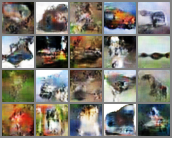
(a) SGDA ($67.4$)

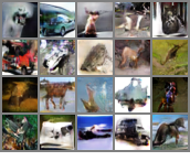
(b) clipped-SGDA ($19.7$)

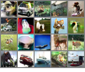
(c) clipped-SEG ($25.3$)

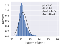
(d) Generator

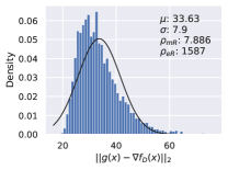
(e) Discriminator

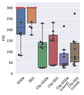
(f) Hyperparameters

Figure 2: (a, b, c) Random samples generated from the best CIFAR models trained (100k steps) by the specified optimizers, with their corresponding FIDs. (d, e) Gradient noise histograms for WGAN-GP upon initialization; a Gaussian was fit using maximum likelihood estimation to showcase the tail of the distribution. $p_{mR}$ is a value estimating the “heavy tailed-ness” of the distribution. (f) The best (lowest) FID scores obtained within the first 35k (out of 100k) training iterations for the same WGAN-GP model trained on CIFAR-10 when sweeping over different hyperparameters. Red points indicate that the run diverged, meaning that the loss becomes NaN. Note that we clip the FID for diverged runs to 300 to not skew the boxplot. Boxes are the quartiles of data.

WGAN-GP. In this section, we focus on the ResNet architecture proposed in Gulrajani et al. [2017], and we adapt our code from a publicly available WGAN-GP implementation. We first compute the gradient noise distribution and validate if it is heavy-tailed. Taking the fixed randomly initialized weights, we iterate through 1000 steps (without parameter updates) to compute the noise norm for each minibatch (sample with replacement as in normal GAN training). We show the distributions for the generator and discriminator in Fig. 2 and also compute $p_{mR}=F_{1.5}(X)$ and $p_{eR}=F_{3}(X)$, where $F_{\lambda}(X)=P(Q_{3}+\lambda(Q_{3}-Q_{1})<X)$, $X$ is the gradient noise distribution, and $Q_{i}$ is the $i^{th}$ quartile. This is a metric introduced by Jordanova and Petkova [2017] to measure how heavy-tailed a distribution is based on the distribution’s quantiles, where $p_{mR}$ and $p_{eR}$ quantify “mild” and “extreme” (right side) heavy tails respectively. A normal distribution should have $p_{mR\mathcal{N}}\approx 0.0035$ and $p_{eR\mathcal{N}}\approx 1.2\times 10^{-6}$. In all tests, we compute the ratios $\rho_{mR}=p_{mR}/p_{mR\mathcal{N}}$ and $\rho_{eR}=p_{eR}/p_{eR\mathcal{N}}$ and empirically find that we at least have mild heavy tails, and sometimes extremely heavy tails.

We train the ResNet generator on CIFAR-10 with SGDA/SEG, and clipped-SGDA/SEG. We use the default architectures and training parameters specified in Gulrajani et al. [2017] ($\lambda_{GP}=10$, $n_{dis}=5$, learning rate decayed linearly to 0 over 100k steps), with the exception of doubling the feature map of the generator. The clipped methods are implemented as standard gradient norm clipping, applied after computing the gradient penalty term for the critic. In addition to norm clipping, we also test coordinate-wise gradient clipping, which is more common in practice [Goodfellow et al., 2016b]. For all methods, we tune the learning rates and clipping threshold where applicable. We do not use momentum following a standard practice for GAN training [Gidel et al., 2019b].

We find that clipped methods outperform regular SGDA and SEG. In addition to helping prevent exploding gradients, clipped methods achieve a better Fréchet inception distance (FID) score [Heusel et al., 2017]; the best FID obtained for clipped methods is $19.65$ in comparison to $67.37$ for regular SGDA, both trained for 100k steps. A summary of FIDs obtained during hyperparameter tuning is shown Fig. 2, where the best FID score obtained in the first 35k iterations is drawn for each hyperparameter configuration and optimization method. At a high level, we do a log-space sweep over $[2\mathrm{e-}5,0.2]$ for the learning rates, $[10^{-1},10]$ for the norm-clip parameter, and $[10^{-3},10^{-1}]$ for the coordinate clip parameter (with some exceptions) – please refer to § E for further details. We also show the evolution of the gradient noise histograms during training for SGD and clipped-SGDA in Fig. 4. Note that for regular SGD, the noise distribution remains heavy tailed and does not appear to change much throughout training. In contrast, the noise histograms for clipped-SGDA (in particular the generator) seem to develop lighter tails during training.

StyleGAN2. We extend our experiments to StyleGAN2, but limit our scope to clipped-SGDA with coordinate clipping as coordinate clipped-SGDA generally performs the best, and StyleGAN2 is expensive to train. We train on FFHQ downsampled to $128\times 128$ pixels, and use the recommended StyleGAN2 hyperparameter configuration for this resolution (batch size $=32$, $\gamma=0.1024$, map depth $=2$, channel multiplier $=16384$), see further experimental details in § E. We obtain the gradient noise histograms at initialization and for the best trained clipped-SGDA from the hyperparameter sweep and once again observe heavy tails (especially in the discriminator, see Fig. 3). We find that all regular SGDA runs fail to learn anything meaningful, with FID scores fluctuating around $320$ and only able to generate noise. In contrast, while there is a clear gap in quality when compared to what StyleGAN2 is capable of, a model trained with clipped-SGDA with appropriately set hyperparameters is able to produce images that distinctly resemble faces (see Fig. 3).

Generator Discriminator
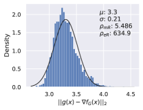
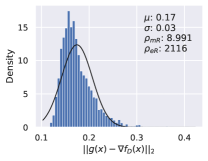
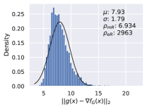
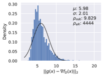
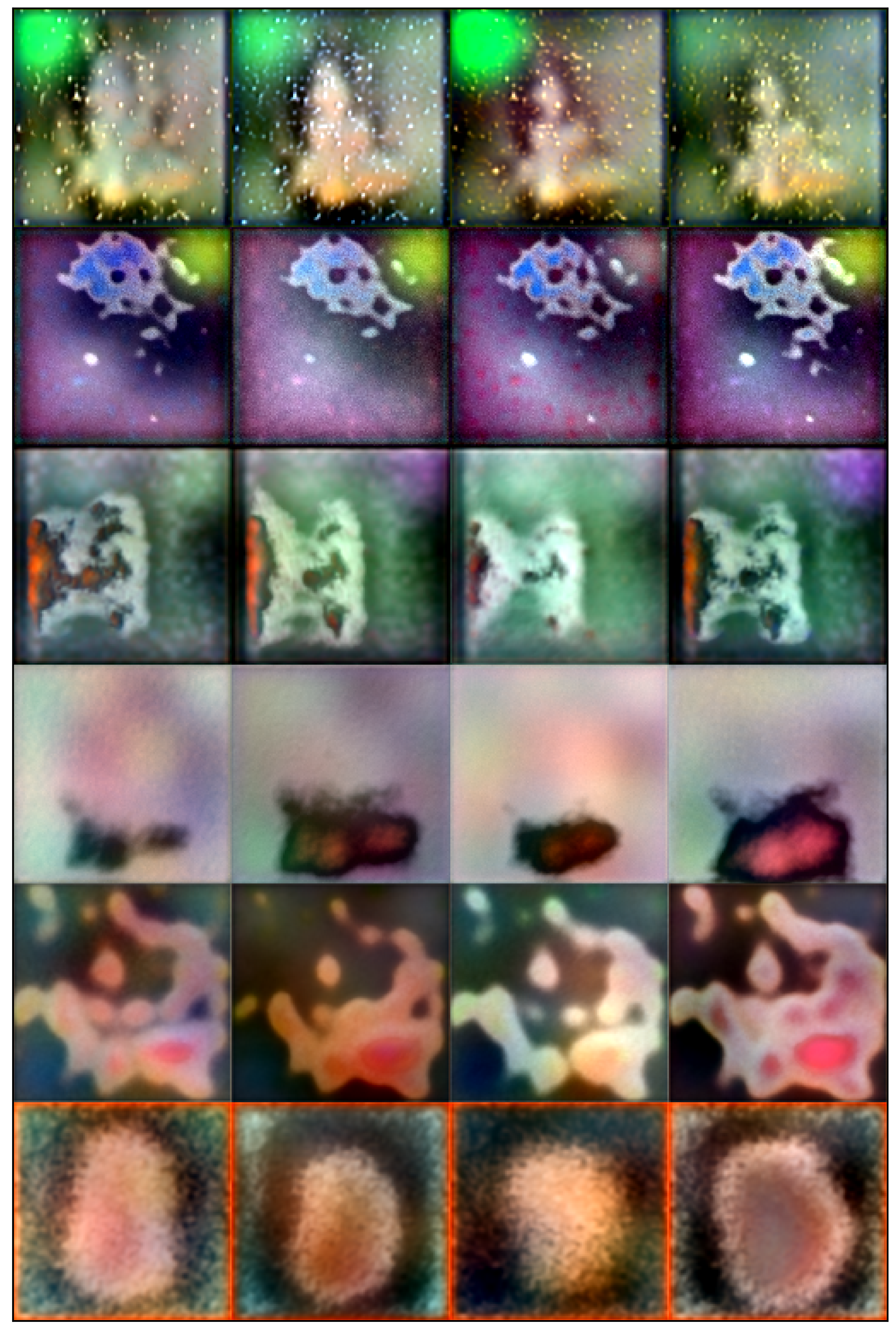
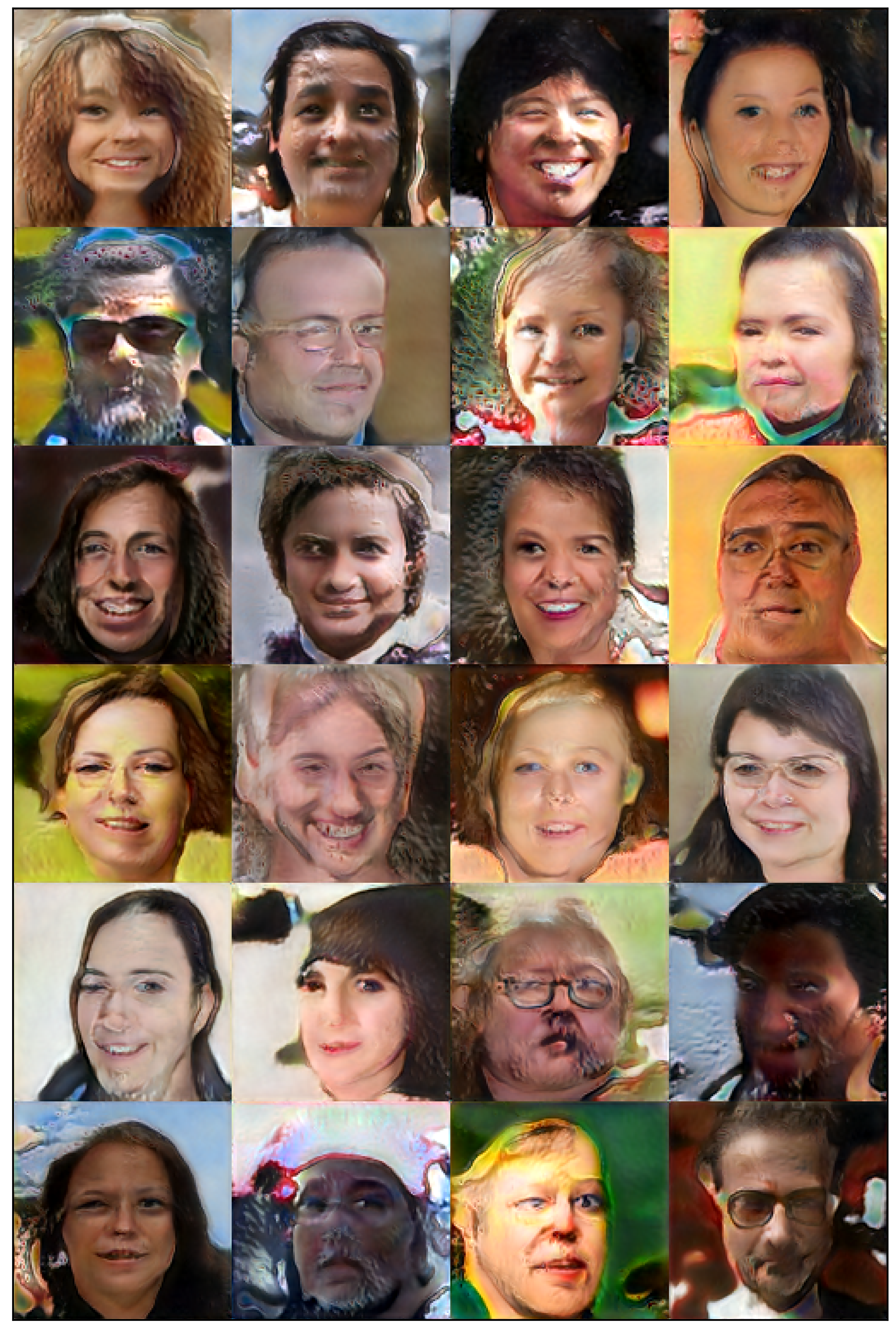
	(a) Initialization	(b) clipped-SGDA	(c) SGDA	(d) clipped-SGDA

Figure 3: (a) Gradient noise histograms for StyleGAN2 at random initialization. (b) Gradient noise histograms for StyleGAN2 trained with clipped-SGDA. (c) Random samples generated from several models trained with SGDA with different learning rates (FID $>300$). Each row corresponds to a different trained model, and all of our attempts to train StyleGAN2 with SGDA produced similar results. (d) Random samples generated from the best clipped-SGDA trained model (FID $=72.68$).

Generator
Discriminator
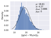
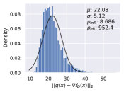
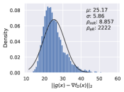
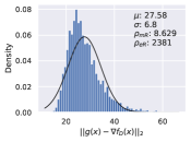
Generator
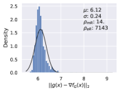
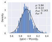
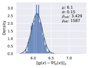
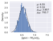
Discriminator
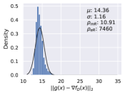
	20000 steps	40000 steps	80000 steps	100000 steps

Figure 4: Evolution of gradient noise histograms for a WGAN-GP model. The top two rows are trained with SGDA, and the bottom two rows are trained with clipped-SGDA.

Checklist

1. For all authors…

   1. Do the main claims made in the abstract and introduction accurately reflect the paper’s contributions and scope? [Yes]

   2. Did you describe the limitations of your work? [Yes] We explicitly formulate all assumptions in § 1.1.

   3. Did you discuss any potential negative societal impacts of your work? [N/A] Our work is mainly theoretical.

   4. Have you read the ethics review guidelines and ensured that your paper conforms to them? [Yes]

2. If you are including theoretical results…

   1. Did you state the full set of assumptions of all theoretical results? [Yes] We explicitly formulate all assumptions in § 1.1.

   2. Did you include complete proofs of all theoretical results? [Yes] Proofs are included in the Appendix.

3. If you ran experiments…

   1. Did you include the code, data, and instructions needed to reproduce the main experimental results (either in the supplemental material or as a URL)? [Yes]

   2. Did you specify all the training details (e.g., data splits, hyperparameters, how they were chosen)? [Yes]

   3. Did you report error bars (e.g., with respect to the random seed after running experiments multiple times)? [No] Training GANs is computationally expensive and we did not aim at achieving SOTA FID.

   4. Did you include the total amount of compute and the type of resources used (e.g., type of GPUs, internal cluster, or cloud provider)? [Yes]

4. If you are using existing assets (e.g., code, data, models) or curating/releasing new assets…

   1. If your work uses existing assets, did you cite the creators? [Yes]

   2. Did you mention the license of the assets? [N/A]

   3. Did you include any new assets either in the supplemental material or as a URL? [N/A]

   4. Did you discuss whether and how consent was obtained from people whose data you’re using/curating? [N/A]

   5. Did you discuss whether the data you are using/curating contains personally identifiable information or offensive content? [N/A]

5. If you used crowdsourcing or conducted research with human subjects…

   1. Did you include the full text of instructions given to participants and screenshots, if applicable? [N/A]

   2. Did you describe any potential participant risks, with links to Institutional Review Board (IRB) approvals, if applicable? [N/A]

   3. Did you include the estimated hourly wage paid to participants and the total amount spent on participant compensation? [N/A]

Contents

1. 1 Introduction
   1. 1.1 Technical Preliminaries
   2. 1.2 Our Contributions
   3. 1.3 Closely Related Work
2. 2 Clipped Stochastic Extragradient
3. 3 Clipped Stochastic Gradient Descent-Ascent
4. 4 Experiments
5. A Further Related Work
6. B Auxiliary Results
7. C Clipped Stochastic Extragradient: Missing Proofs and Details
   1. C.1 Monotone Case
   2. C.2 Star-Negative Comonotone Case
   3. C.3 Quasi-Strongly Monotone Case
8. D Clipped Stochastic Gradient Descent-Ascent: Missing Proofs and Details
   1. D.1 Monotone Star-Cocoercive Case
   2. D.2 Star-Cocoercive Case
   3. D.3 Quasi-Strongly Monotone Star-Cocoercive Case
9. E Extra Experiments
   1. E.1 WGAN-GP
   2. E.2 StyleGAN2

Appendix A Further Related Work

Convergence in expectation. Convergence in expectation of stochastic methods for solving VIPs is relatively well-studied in the literature. In particular, versions of SEG are studied under bounded variance [Beznosikov et al., 2020, Hsieh et al., 2020], smoothness of stochastic realizations [Mishchenko et al., 2020], and more refined assumptions unifying previously used ones [Gorbunov et al., 2022a]. Recent advances on the in-expectation convergence of SGDA are obtained in [Loizou et al., 2021, Beznosikov et al., 2022].

Gradient clipping. In the context of solving minimization problems, gradient clipping [Pascanu et al., 2013] and normalization [Hazan et al., 2015] are known to have a number of favorable properties such as practical robustness to the rapid changes of the loss function [Goodfellow et al., 2016a], provable convergence for structured non-smooth problems with polynomial growth Zhang et al. [2020a], Mai and Johansson [2021] and for the problems with heavy-tailed noise in convex [Nazin et al., 2019, Gorbunov et al., 2020, 2021] and non-convex cases [Zhang et al., 2020b, Cutkosky and Mehta, 2021]. Our work makes a further step towards a better understanding of gradient clipping and is the first to study the theoretical convergence of clipped first-order stochastic methods for VIPs.

Structured non-monotonicity. There is a noticeable growing interest of the community in studying the theoretical convergence guarantees of deterministic methods for solving VIP with non-monotone operators $F(x)$ having a certain structure, e.g., negative comonotonicty [Diakonikolas et al., 2021, Lee and Kim, 2021, Böhm, 2022], quasi-strong monotonicity [Song et al., 2020, Mertikopoulos and Zhou, 2019] and/or star-cocoercivity [Loizou et al., 2021, Gorbunov et al., 2022b, a, Beznosikov et al., 2022]. In the context of stochastic VIPs, SEG (with different extrapolation and update stepsizes) is analyzed under negative comonotonicity by Diakonikolas et al. [2021] and under quasi-strong monotonicity by Gorbunov et al. [2022a], while SGDA is studied under quasi-strong monotonicity and/or star-cocoercivity by [Loizou et al., 2021, Beznosikov et al., 2022]. These results establish in-expectation convergence rates. Our paper continues this line of works and provides the first high-probability analysis of stochastic methods for solving VIPs with structured non-monotonicity.

Appendix B Auxiliary Results

Useful inequalities.

For all $a,b\in\mathbb{R}^{d}$ and $\alpha>0$ the following relations hold:

$$2\langle a,b\rangle = \|a\|^{2}+\|b\|^{2}-\|a-b\|^{2},$$ (4)

$$\|a+b\|^{2} \leq 2\|a\|^{2}+2\|b\|^{2},$$ (5)

$$-\|a-b\|^{2} \leq -\frac{1}{2}\|a\|^{2}+\|b\|^{2}.$$ (6)

Bernstein inequality.

In our proofs, we rely on the following lemma known as Bernstein inequality for martingale differences [Bennett, 1962, Dzhaparidze and Van Zanten, 2001, Freedman et al., 1975].

Lemma B.1.

Let the sequence of random variables $\{X_{i}\}_{i\geq 1}$ form a martingale difference sequence, i.e. $\mathbb{E}\left[X_{i}\mid X_{i-1},\ldots,X_{1}\right]=0$ for all $i\geq 1$. Assume that conditional variances $\sigma_{i}^{2}\stackrel{{\scriptstyle\text{def}}}{{=}}\mathbb{E}\left[X_{i}^{2}\mid X_{i-1},\ldots,X_{1}\right]$ exist and are bounded and assume also that there exists deterministic constant $c>0$ such that $|X_{i}|\leq c$ almost surely for all $i\geq 1$. Then for all $b>0$, $G>0$ and $n\geq 1$

$$\mathbb{P}\left\{\Big{|}\sum\limits_{i=1}^{n}X_{i}\Big{|}>b\text{ and }\sum\limits_{i=1}^{n}\sigma_{i}^{2}\leq G\right\}\leq 2\exp\left(-\frac{b^{2}}{2G+\nicefrac{{2cb}}{{3}}}\right).$$ (7)

Bias and variance of clipped stochastic vector.

We also use the following properties of clipped stochastic estimators from [Gorbunov et al., 2020].

Lemma B.2 (Simplified version of Lemma F.5 from [Gorbunov et al., 2020]).

Let $X$ be a random vector in $\mathbb{R}^{d}$ and $\widetilde{X}=\texttt{clip}(X,\lambda)$. Then,

$$\left\|\widetilde{X}-\mathbb{E}[\widetilde{X}]\right\|\leq 2\lambda.$$ (8)

Moreover, if for some $\sigma\geq 0$

$$\mathbb{E}[X]=x\in\mathbb{R}^{d},\quad\mathbb{E}[\|X-x\|^{2}]\leq\sigma^{2}$$ (9)

and $x\leq\nicefrac{{\lambda}}{{2}}$, then

$$\left\|\mathbb{E}[\widetilde{X}]-x\right\| \leq \frac{4\sigma^{2}}{\lambda},$$ (10)

$$\mathbb{E}\left[\left\|\widetilde{X}-x\right\|^{2}\right] \leq 18\sigma^{2},$$ (11)

$$\mathbb{E}\left[\left\|\widetilde{X}-\mathbb{E}[\widetilde{X}]\right\|^{2}\right] \leq 18\sigma^{2}.$$ (12)

Proof.

The proof of this lemma is identical to the original one, since Gorbunov et al. [2020] rely only on $\widetilde{X}=\texttt{clip}(X,\lambda)$ to derive (8), and to prove (10)-(12) they use only (9), $\widetilde{X}=\texttt{clip}(X,\lambda)$ and $x\leq\nicefrac{{\lambda}}{{2}}$ ∎

Appendix C Clipped Stochastic Extragradient: Missing Proofs and Details

C.1 Monotone Case

Lemma C.1.

Let Assumptions 1.1, 1.2, 1.3 hold for $Q=B_{4R}(x^{*})$, where $R\geq R_{0}\stackrel{{\scriptstyle\text{def}}}{{=}}\|x^{0}-x^{*}\|$, and $\gamma_{1}=\gamma_{2}=\gamma$, $0<\gamma\leq\nicefrac{{1}}{{\sqrt{2}L}}$. If $x^{k}$ and $\widetilde{x}^{k}$ lie in $B_{4R}(x^{*})$ for all $k=0,1,\ldots,K$ for some $K\geq 0$, then for all $u\in B_{4R}(x^{*})$ the iterates produced by clipped-SEG satisfy

$$\langle F(u),\widetilde{x}^{K}_{\texttt{avg}}-u\rangle \leq \frac{\|x^{0}-u\|^{2}-\|x^{K+1}-u\|^{2}}{2\gamma(K+1)}+\frac{\gamma}{2(K+1)}\sum\limits_{k=0}^{K}\left(\|\theta_{k}\|^{2}+2\|\omega_{k}\|^{2}\right)$$ (13)

$$\quad+\frac{1}{K+1}\sum\limits_{k=0}^{K}\langle x^{k}-u-\gamma F(\widetilde{x}^{k}),\theta_{k}\rangle,$$

$$\widetilde{x}^{K}_{\texttt{avg}} \stackrel{{\scriptstyle\text{def}}}{{=}} \frac{1}{K+1}\sum\limits_{k=0}^{K}\widetilde{x}^{k},$$ (14)

$$\theta_{k} \stackrel{{\scriptstyle\text{def}}}{{=}} F(\widetilde{x}^{k})-\widetilde{F}_{\boldsymbol{\xi}_{2}^{k}}(\widetilde{x}^{k}),$$ (15)

$$\omega_{k} \stackrel{{\scriptstyle\text{def}}}{{=}} F(x^{k})-\widetilde{F}_{\boldsymbol{\xi}_{1}^{k}}(x^{k}).$$ (16)

Proof.

Using the update rule of clipped-SEG, for all $u\in B_{4R}(x^{*})$ we obtain

$$\|x^{k+1}-u\|^{2} = \|x^{k}-u\|^{2}-2\gamma\langle x^{k}-u,\widetilde{F}_{\boldsymbol{\xi}_{2}^{k}}(\widetilde{x}^{k})\rangle+\gamma^{2}\|\widetilde{F}_{\boldsymbol{\xi}_{2}^{k}}(\widetilde{x}^{k})\|^{2}$$

$$= \|x^{k}-u\|^{2}-2\gamma\langle x^{k}-u,F(\widetilde{x}^{k})\rangle+2\gamma\langle x^{k}-u,\theta_{k}\rangle$$

$$\quad+\gamma^{2}\|F(\widetilde{x}^{k})\|^{2}-2\gamma^{2}\langle F(\widetilde{x}^{k}),\theta_{k}\rangle+\gamma^{2}\|\theta_{k}\|^{2}$$

$$= \|x^{k}-u\|^{2}-2\gamma\langle\widetilde{x}^{k}-u,F(\widetilde{x}^{k})\rangle-2\gamma\langle x^{k}-\widetilde{x}^{k},F(\widetilde{x}^{k})\rangle$$

$$\quad+2\gamma\langle x^{k}-u-\gamma F(\widetilde{x}^{k}),\theta_{k}\rangle+\gamma^{2}\|F(\widetilde{x}^{k})\|^{2}+\gamma^{2}\|\theta_{k}\|^{2}$$

$$\overset{\eqref{eq:monotonicity}}{\leq} \|x^{k}-u\|^{2}-2\gamma\langle\widetilde{x}^{k}-u,F(u)\rangle-2\gamma^{2}\langle\widetilde{F}_{\boldsymbol{\xi}_{1}^{k}}(x^{k}),F(\widetilde{x}^{k})\rangle$$

$$\quad+2\gamma\langle x^{k}-u-\gamma F(\widetilde{x}^{k}),\theta_{k}\rangle+\gamma^{2}\|F(\widetilde{x}^{k})\|^{2}+\gamma^{2}\|\theta_{k}\|^{2}$$

$$\overset{\eqref{eq:inner_product_representation}}{=} \|x^{k}-u\|^{2}-2\gamma\langle\widetilde{x}^{k}-u,F(u)\rangle$$

$$\quad+\gamma^{2}\|\widetilde{F}_{\boldsymbol{\xi}_{1}^{k}}(x^{k})-F(\widetilde{x}^{k})\|^{2}-\gamma^{2}\|F(\widetilde{x}^{k})\|^{2}-\gamma^{2}\|\widetilde{F}_{\boldsymbol{\xi}_{1}^{k}}(x^{k})\|^{2}$$

$$\quad+2\gamma\langle x^{k}-u-\gamma F(\widetilde{x}^{k}),\theta_{k}\rangle+\gamma^{2}\|F(\widetilde{x}^{k})\|^{2}+\gamma^{2}\|\theta_{k}\|^{2}$$

$$\overset{\eqref{eq:a_plus_b}}{\leq} \|x^{k}-u\|^{2}-2\gamma\langle\widetilde{x}^{k}-u,F(u)\rangle$$

$$\quad+2\gamma^{2}\|\omega_{k}\|^{2}+2\gamma^{2}\|F(x^{k})-F(\widetilde{x}^{k})\|^{2}-\gamma^{2}\|\widetilde{F}_{\boldsymbol{\xi}_{1}^{k}}(x^{k})\|^{2}$$

$$\quad+2\gamma\langle x^{k}-u-\gamma F(\widetilde{x}^{k}),\theta_{k}\rangle+\gamma^{2}\|\theta_{k}\|^{2}$$

$$\overset{\eqref{eq:Lipschitzness}}{\leq} \|x^{k}-u\|^{2}-2\gamma\langle\widetilde{x}^{k}-u,F(u)\rangle-\gamma^{2}\left(1-2\gamma^{2}L^{2}\right)\|\widetilde{F}_{\boldsymbol{\xi}_{1}^{k}}(x^{k})\|^{2}$$

$$\quad+2\gamma\langle x^{k}-u-\gamma F(\widetilde{x}^{k}),\theta_{k}\rangle+\gamma^{2}\|\theta_{k}\|^{2}+2\gamma^{2}\|\omega_{k}\|^{2}$$

where in the last step we additionally use $x^{k}-\widetilde{x}^{k}=\gamma\widetilde{F}_{\boldsymbol{\xi}_{1}^{k}}(x^{k})$ after the application of Lipschitzness of $F$. Since $\gamma\leq\nicefrac{{1}}{{\sqrt{2}L}}$, we have $\gamma^{2}\left(1-2\gamma^{2}L^{2}\right)\|\widetilde{F}_{\boldsymbol{\xi}_{1}^{k}}(x^{k})\|^{2}\geq 0$, implying

$$2\gamma\langle F(u),\widetilde{x}^{k}-u\rangle \leq \|x^{k}-u\|^{2}-\|x^{k+1}-u\|^{2}+\gamma^{2}\left(\|\theta_{k}\|^{2}+2\|\omega_{k}\|^{2}\right)$$

$$\quad+2\gamma\langle x^{k}-u-\gamma F(\widetilde{x}^{k}),\theta_{k}\rangle.$$

Finally, we sum up the above inequality for $k=0,1,\ldots,K$ and divide both sides of the result by $2\gamma(K+1)$:

$$\langle F(u),\widetilde{x}^{K}_{\texttt{avg}}-u\rangle = \frac{1}{K+1}\sum\limits_{k=0}^{K}\langle F(u),\widetilde{x}^{k}-u\rangle$$

$$\leq \frac{1}{2\gamma(K+1)}\sum\limits_{k=0}^{K}\left(\|x^{k}-u\|^{2}-\|x^{k+1}-u\|^{2}\right)+\frac{\gamma}{2(K+1)}\sum\limits_{k=0}^{K}\|\theta_{k}\|^{2}$$

$$\quad+\frac{1}{K+1}\sum\limits_{k=0}^{K}\langle x^{k}-u-\gamma F(\widetilde{x}^{k}),\theta_{k}\rangle+\frac{\gamma}{K+1}\sum\limits_{k=0}^{K}\|\omega_{k}\|^{2}$$

$$= \frac{\|x^{0}-u\|^{2}-\|x^{K+1}-u\|^{2}}{2\gamma(K+1)}+\frac{\gamma}{2(K+1)}\sum\limits_{k=0}^{K}\left(\|\theta_{k}\|^{2}+2\|\omega_{k}\|^{2}\right)$$

$$\quad+\frac{1}{K+1}\sum\limits_{k=0}^{K}\langle x^{k}-u-\gamma F(\widetilde{x}^{k}),\theta_{k}\rangle.$$

This concludes the proof. ∎

Theorem C.1.

Let Assumptions 1.1, 1.2, 1.3 hold for $Q=B_{4R}(x^{*})$, where $R\geq R_{0}\stackrel{{\scriptstyle\text{def}}}{{=}}\|x^{0}-x^{*}\|$, and $\gamma_{1}=\gamma_{2}=\gamma$,

$$0<\gamma \leq \frac{1}{160L\ln\tfrac{6(K+1)}{\beta}},$$ (17)

$$\lambda_{1,k}=\lambda_{2,k}\equiv\lambda = \frac{R}{20\gamma\ln\tfrac{6(K+1)}{\beta}},$$ (18)

$$m_{1,k}=m_{2,k}\equiv m \geq \max\left\{1,\frac{10800(K+1)\gamma^{2}\sigma^{2}\ln\tfrac{6(K+1)}{\beta}}{R^{2}}\right\},$$ (19)

for some $K\geq 0$ and $\beta\in(0,1]$ such that $\ln\tfrac{6(K+1)}{\beta}\geq 1$. Then, after $K$ iterations the iterates produced by clipped-SEG with probability at least $1-\beta$ satisfy

$$\texttt{Gap}_{R}(\widetilde{x}_{\texttt{avg}}^{K})\leq\frac{9R^{2}}{2\gamma(K+1)},$$ (20)

where $\widetilde{x}_{\texttt{avg}}^{K}$ is defined in (14).

Proof.

We introduce new notation: $R_{k}=\|x^{k}-x^{*}\|$ for all $k\geq 0$. The proof is based on deriving via induction that $R_{k}^{2}\leq\tilde{C}R^{2}$ for some numerical constant $\tilde{C}>0$. In particular, for each $k=0,\ldots,K+1$ we define probability event $E_{k}$ as follows: inequalities

$$\underbrace{\max\limits_{u\in B_{R}(x^{*})}\!\left\{\!\|x^{0}-u\|^{2}+2\gamma\sum\limits_{l=0}^{t-1}\langle x^{l}-u-\gamma F(\widetilde{x}^{l}),\theta_{l}\rangle+\gamma^{2}\sum\limits_{l=0}^{t-1}\left(\|\theta_{l}\|^{2}+2\|\omega_{l}\|^{2}\right)\!\right\}}_{A_{t}}\leq 9R^{2},$$ (21)

$$\left\|\gamma\sum\limits_{l=0}^{t-1}\theta_{l}\right\|\leq R$$ (22)

hold for $t=0,1,\ldots,k$ simultaneously. Our goal is to prove that $\mathbb{P}\{E_{k}\}\geq 1-\nicefrac{{k\beta}}{{(K+1)}}$ for all $k=0,1,\ldots,K+1$. We use the induction to show this statement. For $k=0$ the statement is trivial since $\|x^{0}-u\|^{2}\leq 2\|x^{0}-x^{*}\|^{2}+2\|x^{*}-u\|^{2}\leq 4R^{2}\leq 9R^{2}$ and $\|\gamma\sum_{l=0}^{k-1}\theta_{l}\|=0$ for any $u\in B_{R}(x^{*})$. Next, assume that the statement holds for $k=T-1\leq K$, i.e., we have $\mathbb{P}\{E_{T-1}\}\geq 1-\nicefrac{{(T-1)\beta}}{{(K+1)}}$. We need to prove that $\mathbb{P}\{E_{T}\}\geq 1-\nicefrac{{T\beta}}{{(K+1)}}$. First of all, we show that probability event $E_{T-1}$ implies $R_{t}\leq 3R$ for all $t=0,1,\ldots,T$. For $t=0$ we already proved it. Next, assume that we have $R_{t}\leq 3R$ for all $t=0,1,\ldots,t^{\prime}$, where $t^{\prime}<T$. Then, for all $t=0,1,\ldots,t^{\prime}$ we have

$$\|\widetilde{x}^{t}-x^{*}\| = \|x^{t}-x^{*}-\gamma\widetilde{F}_{\boldsymbol{\xi}_{1}^{t}}(x^{t})\|\leq\|x^{t}-x^{*}\|+\gamma\|\widetilde{F}_{\boldsymbol{\xi}_{1}^{t}}(x^{t})\|$$ (23)

$$\leq \|x^{t}-x^{*}\|+\gamma\lambda\overset{\eqref{eq:lambda_SEG}}{\leq}3R+\frac{R}{20\ln\frac{6(K+1)}{\beta}}\leq 4R,$$

i.e., $\widetilde{x}^{t}\in B_{4R}(x^{*})$. This means that the assumptions of Lemma C.1 hold and we have that probability event $E_{T-1}$ implies

$$\max\limits_{u\in B_{R}(x^{*})}\left\{2\gamma(t^{\prime}+1)\langle F(u),\widetilde{x}^{t^{\prime}}_{\texttt{avg}}-u\rangle+\|x^{t^{\prime}+1}-u\|^{2}\right\}$$

$$\leq\max\limits_{u\in B_{R}(x^{*})}\!\left\{\!\|x^{0}-u\|^{2}+2\gamma\sum\limits_{l=0}^{t^{\prime}-1}\langle x^{l}-u-\gamma F(\widetilde{x}^{l}),\theta_{l}\rangle\!\right\}$$

$$+\gamma^{2}\sum\limits_{l=0}^{t^{\prime}-1}\left(\|\theta_{l}\|^{2}+2\|\omega_{l}\|^{2}\right)$$

$$\overset{\eqref{eq:induction_inequality_1_SEG}}{\leq}9R^{2},$$

meaning that

$$\|x^{t^{\prime}+1}-x^{*}\|^{2} \leq \max\limits_{u\in B_{R}(x^{*})}\left\{2\gamma(t^{\prime}+1)\langle F(u),\widetilde{x}^{t^{\prime}}_{\texttt{avg}}-u\rangle+\|x^{t^{\prime}+1}-u\|^{2}\right\}$$

$$\leq 9R^{2},$$

i.e., $R_{t^{\prime}+1}\leq 3R$. That is, we proved that probability event $E_{T-1}$ implies $R_{t}\leq 3R$ and

$$\max\limits_{u\in B_{R}(x^{*})}\left\{2\gamma(t+1)\langle F(u),\widetilde{x}^{t}_{\texttt{avg}}-u\rangle+\|x^{t+1}-u\|^{2}\right\}\leq 9R^{2}$$ (24)

for all $t=0,1,\ldots,T$. Moreover, in view of (23) $E_{T-1}$ also implies that $\|\widetilde{x}^{t}-x^{*}\|\leq 4R$ for all $t=0,1,\ldots,T$. Using this, we derive that $E_{T-1}$ implies

$$\|x^{t}-x^{*}-\gamma F(\widetilde{x}^{t})\| \leq \|x^{t}-x^{*}\|+\gamma\|F(\widetilde{x}^{t})\|\overset{\eqref{eq:Lipschitzness}}{\leq}3R+\gamma L\|\widetilde{x}^{t}-x^{*}\|$$ (25)

$$\overset{\eqref{eq:gap_thm_SEG_technical_1}}{\leq} 3R+4R\gamma L\overset{\eqref{eq:gamma_SEG}}{\leq}5R,$$

for all $t=0,1,\ldots,T$. Consider random vectors

$$\eta_{t}=\begin{cases}x^{t}-x^{*}-\gamma F(\widetilde{x}^{t}),&\text{if }\|x^{t}-x^{*}-\gamma F(\widetilde{x}^{t})\|\leq 5R,\\ 0,&\text{otherwise,}\end{cases}$$

for all $t=0,1,\ldots,T$. We notice that $\eta_{t}$ is bounded with probability $1$:

$$\|\eta_{t}\|\leq 5R$$ (26)

for all $t=0,1,\ldots,T$. Moreover, in view of (25), probability event $E_{T-1}$ implies $\eta_{t}=x^{t}-x^{*}-\gamma F(\widetilde{x}^{t})$ for all $t=0,1,\ldots,T$. Therefore, $E_{T-1}$ implies

$$A_{T} = \max\limits_{u\in B_{R}(x^{*})}\left\{\|x^{0}-u\|^{2}+2\gamma\sum\limits_{l=0}^{T-1}\langle x^{*}-u,\theta_{l}\rangle\right\}$$

$$\quad+2\gamma\sum\limits_{l=0}^{T-1}\langle x^{l}-x^{*}-\gamma F(\widetilde{x}^{l}),\theta_{l}\rangle+\gamma^{2}\sum\limits_{l=0}^{T-1}\left(\|\theta_{l}\|^{2}+2\|\omega_{l}\|^{2}\right)$$

$$\leq 4R^{2}+2\gamma\max\limits_{u\in B_{R}(x^{*})}\left\{\left\langle x^{*}-u,\sum\limits_{l=0}^{T-1}\theta_{l}\right\rangle\right\}$$

$$\quad+2\gamma\sum\limits_{l=0}^{T-1}\langle\eta_{l},\theta_{l}\rangle+\gamma^{2}\sum\limits_{l=0}^{T-1}\left(\|\theta_{l}\|^{2}+2\|\omega_{l}\|^{2}\right)$$

$$= 4R^{2}+2\gamma R\left\|\sum\limits_{l=0}^{T-1}\theta_{l}\right\|+2\gamma\sum\limits_{l=0}^{T-1}\langle\eta_{l},\theta_{l}\rangle+\gamma^{2}\sum\limits_{l=0}^{T-1}\left(\|\theta_{l}\|^{2}+2\|\omega_{l}\|^{2}\right),$$

where $A_{T}$ is defined in (21). To continue our derivation we introduce new notation:

$$\theta_{l}^{u}\stackrel{{\scriptstyle\text{def}}}{{=}}\mathbb{E}_{\boldsymbol{\xi}_{2}^{l}}\left[\widetilde{F}_{\boldsymbol{\xi}_{2}^{l}}(\widetilde{x}^{l})\right]-\widetilde{F}_{\boldsymbol{\xi}_{2}^{l}}(\widetilde{x}^{l}),\quad\theta_{l}^{b}\stackrel{{\scriptstyle\text{def}}}{{=}}F(\widetilde{x}^{l})-\mathbb{E}_{\boldsymbol{\xi}_{2}^{l}}\left[\widetilde{F}_{\boldsymbol{\xi}_{2}^{l}}(\widetilde{x}^{l})\right],$$ (27)

$$\omega_{l}^{u}\stackrel{{\scriptstyle\text{def}}}{{=}}\mathbb{E}_{\boldsymbol{\xi}_{1}^{l}}\left[\widetilde{F}_{\boldsymbol{\xi}_{1}^{l}}(x^{l})\right]-\widetilde{F}_{\boldsymbol{\xi}_{1}^{l}}(x^{l}),\quad\omega_{l}^{b}\stackrel{{\scriptstyle\text{def}}}{{=}}F(x^{l})-\mathbb{E}_{\boldsymbol{\xi}_{1}^{l}}\left[\widetilde{F}_{\boldsymbol{\xi}_{1}^{l}}(x^{l})\right],$$ (28)

for all $l=0,\ldots,T-1$. By definition we have $\theta_{l}=\theta_{l}^{u}+\theta_{l}^{b}$, $\omega_{l}=\omega_{l}^{u}+\omega_{l}^{b}$ for all $l=0,\ldots,T-1$. Using the introduced notation, we continue our derivation as follows: $E_{T-1}$ implies

$$A_{T} \overset{\eqref{eq:a_plus_b}}{\leq} 4R^{2}+2\gamma R\left\|\sum\limits_{l=0}^{T-1}\theta_{l}\right\|+\underbrace{2\gamma\sum\limits_{l=0}^{T-1}\langle\eta_{l},\theta_{l}^{u}\rangle}_{\text{\char 172}}+\underbrace{2\gamma\sum\limits_{l=0}^{T-1}\langle\eta_{l},\theta_{l}^{b}\rangle}_{\text{\char 173}}$$ (29)

$$\quad+\underbrace{2\gamma^{2}\sum\limits_{l=0}^{T-1}\left(\mathbb{E}_{\boldsymbol{\xi}_{2}^{l}}\left[\|\theta_{l}^{u}\|^{2}\right]+2\mathbb{E}_{\boldsymbol{\xi}_{1}^{l}}\left[\|\omega_{l}^{u}\|^{2}\right]\right)}_{\text{\char 174}}$$

$$\quad+\underbrace{2\gamma^{2}\sum\limits_{l=0}^{T-1}\left(\|\theta_{l}^{u}\|^{2}+2\|\omega_{l}^{u}\|^{2}-\mathbb{E}_{\boldsymbol{\xi}_{2}^{l}}\left[\|\theta_{l}^{u}\|^{2}\right]-2\mathbb{E}_{\boldsymbol{\xi}_{1}^{l}}\left[\|\omega_{l}^{u}\|^{2}\right]\right)}_{\text{\char 175}}$$

$$\quad+\underbrace{2\gamma^{2}\sum\limits_{l=0}^{T-1}\left(\|\theta_{l}^{b}\|^{2}+2\|\omega_{l}^{b}\|^{2}\right)}_{\text{\char 176}}$$

The rest of the proof is based on deriving good enough upper bounds for $2\gamma R\left\|\sum_{l=0}^{T-1}\theta_{l}\right\|,\text{\char 172},\text{\char 173},\text{\char 174},\text{\char 175},\text{\char 176}$, i.e., we want to prove that $2\gamma R\left\|\sum_{l=0}^{T-1}\theta_{l}\right\|+\text{\char 172}+\text{\char 173}+\text{\char 174}+\text{\char 175}+\text{\char 176}\leq 5R^{2}$ with high probability.

Before we move on, we need to derive some useful inequalities for operating with $\theta_{l}^{u},\theta_{l}^{b},\omega_{l}^{u},\omega_{l}^{b}$. First of all, Lemma B.2 implies that

$$\|\theta_{l}^{u}\|\leq 2\lambda,\quad\|\omega_{l}^{u}\|\leq 2\lambda$$ (30)

for all $l=0,1,\ldots,T-1$. Next, since $\{\xi_{1}^{i,l}\}_{i=1}^{m}$, $\{\xi_{2}^{i,l}\}_{i=1}^{m}$ are independently sampled from ${\cal D}$, we have $\mathbb{E}_{\boldsymbol{\xi}_{1}^{l}}[F_{\boldsymbol{\xi}_{1}^{l}}(x^{l})]=F(x^{l})$, $\mathbb{E}_{\boldsymbol{\xi}_{2}^{l}}[F_{\boldsymbol{\xi}_{2}^{l}}(\widetilde{x}^{l})]=F(\widetilde{x}^{l})$, and

$$\mathbb{E}_{\boldsymbol{\xi}_{1}^{l}}\left[\|F_{\boldsymbol{\xi}_{1}^{l}}(x^{l})-F(x^{l})\|^{2}\right]=\frac{1}{m^{2}}\sum\limits_{i=1}^{m}\mathbb{E}_{\xi_{1}^{i,l}}\left[\|F_{\xi_{1}^{i,l}}(x^{l})-F(x^{l})\|^{2}\right]\overset{\eqref{eq:UBV}}{\leq}\frac{\sigma^{2}}{m},$$

$$\mathbb{E}_{\boldsymbol{\xi}_{2}^{l}}\left[\|F_{\boldsymbol{\xi}_{2}^{l}}(\widetilde{x}^{l})-F(\widetilde{x}^{l})\|^{2}\right]=\frac{1}{m^{2}}\sum\limits_{i=1}^{m}\mathbb{E}_{\xi_{2}^{i,l}}\left[\|F_{\xi_{2}^{i,l}}(\widetilde{x}^{l})-F(\widetilde{x}^{l})\|^{2}\right]\overset{\eqref{eq:UBV}}{\leq}\frac{\sigma^{2}}{m},$$

for all $l=0,1,\ldots,T-1$. Moreover, probability event $E_{T-1}$ implies

$$\|F(x^{l})\|\overset{\eqref{eq:Lipschitzness}}{\leq}L\|x^{l}-x^{*}\|\leq 3LR\overset{\eqref{eq:gamma_SEG}}{\leq}\frac{R}{40\gamma\ln\tfrac{6(K+1)}{\beta}}\overset{\eqref{eq:lambda_SEG}}{=}\frac{\lambda}{2},$$

$$\|F(\widetilde{x}^{l})\|\overset{\eqref{eq:Lipschitzness}}{\leq}L\|\widetilde{x}^{l}-x^{*}\|\overset{\eqref{eq:gap_thm_SEG_technical_1}}{\leq}4LR\overset{\eqref{eq:gamma_SEG}}{\leq}\frac{R}{40\gamma\ln\tfrac{6(K+1)}{\beta}}\overset{\eqref{eq:lambda_SEG}}{=}\frac{\lambda}{2}$$

for all $l=0,1,\ldots,T-1$. Therefore, in view of Lemma B.2, $E_{T-1}$ implies that

$$\left\|\theta_{l}^{b}\right\|\leq\frac{4\sigma^{2}}{m\lambda},\quad\left\|\omega_{l}^{b}\right\|\leq\frac{4\sigma^{2}}{m\lambda},$$ (31)

$$\mathbb{E}_{\boldsymbol{\xi}_{2}^{l}}\left[\left\|\theta_{l}\right\|^{2}\right]\leq\frac{18\sigma^{2}}{m},\quad\mathbb{E}_{\boldsymbol{\xi}_{1}^{l}}\left[\left\|\omega_{l}\right\|^{2}\right]\leq\frac{18\sigma^{2}}{m},$$ (32)

$$\mathbb{E}_{\boldsymbol{\xi}_{2}^{l}}\left[\left\|\theta_{l}^{u}\right\|^{2}\right]\leq\frac{18\sigma^{2}}{m},\quad\mathbb{E}_{\boldsymbol{\xi}_{1}^{l}}\left[\left\|\omega_{l}^{u}\right\|^{2}\right]\leq\frac{18\sigma^{2}}{m},$$ (33)

for all $l=0,1,\ldots,T-1$.

Upper bound for ①.

Since $\mathbb{E}_{\boldsymbol{\xi}_{2}^{l}}[\theta_{l}^{u}]=0$, we have

$$\mathbb{E}_{\boldsymbol{\xi}_{2}^{l}}\left[2\gamma\langle\eta_{l},\theta_{l}^{u}\rangle\right]=0.$$

Next, the summands in ① are bounded with probability $1$:

$$|2\gamma\langle\eta_{l},\theta_{l}^{u}\rangle|\leq 2\gamma\|\eta_{l}\|\cdot\|\theta_{l}^{u}\|\overset{\eqref{eq:gap_thm_SEG_technical_3},\eqref{eq:theta_omega_magnitude}}{\leq}20\gamma R\lambda\overset{\eqref{eq:lambda_SEG}}{=}\frac{R^{2}}{\ln\tfrac{6(K+1)}{\beta}}\stackrel{{\scriptstyle\text{def}}}{{=}}c.$$ (34)

Moreover, these summands have bounded conditional variances $\sigma_{l}^{2}\stackrel{{\scriptstyle\text{def}}}{{=}}\mathbb{E}_{\boldsymbol{\xi}_{2}^{l}}\left[4\gamma^{2}\langle\eta_{l},\theta_{l}^{u}\rangle^{2}\right]$:

$$\sigma_{l}^{2}\leq\mathbb{E}_{\boldsymbol{\xi}_{2}^{l}}\left[4\gamma^{2}\|\eta_{l}\|^{2}\cdot\|\theta_{l}^{u}\|^{2}\right]\overset{\eqref{eq:gap_thm_SEG_technical_3}}{\leq}100\gamma^{2}R^{2}\mathbb{E}_{\boldsymbol{\xi}_{2}^{l}}\left[\|\theta_{l}^{u}\|^{2}\right].$$ (35)

That is, sequence $\{2\gamma\langle\eta_{l},\theta_{l}^{u}\rangle\}_{l\geq 0}$ is a bounded martingale difference sequence having bounded conditional variances $\{\sigma_{l}^{2}\}_{l\geq 0}$. Applying the Bernstein’s inequality (Lemma B.1) with $X_{l}=2\gamma\langle\eta_{l},\theta_{l}^{u}\rangle$, $c$ defined in (34), $b=R^{2}$, $G=\tfrac{R^{4}}{6\ln\tfrac{6(K+1)}{\beta}}$, we get that

$$\mathbb{P}\left\{|\text{\char 172}|>R^{2}\text{ and }\sum\limits_{l=0}^{T-1}\sigma_{l}^{2}\leq\frac{R^{4}}{6\ln\tfrac{6(K+1)}{\beta}}\right\}\leq 2\exp\left(-\frac{b^{2}}{2G+\nicefrac{{2cb}}{{3}}}\right)=\frac{\beta}{3(K+1)}.$$

In other words, $\mathbb{P}\{E_{\text{\char 172}}\}\geq 1-\tfrac{\beta}{3(K+1)}$, where probability event $E_{\text{\char 172}}$ is defined as

$$E_{\text{\char 172}}=\left\{\text{either}\quad\sum\limits_{l=0}^{T-1}\sigma_{l}^{2}>\frac{R^{4}}{6\ln\tfrac{6(K+1)}{\beta}}\quad\text{or}\quad|\text{\char 172}|\leq R^{2}\right\}.$$ (36)

Moreover, we notice here that probability event $E_{T-1}$ implies that

$$\sum\limits_{l=0}^{T-1}\sigma_{l}^{2}\overset{\eqref{eq:gap_thm_SEG_technical_7}}{\leq}100\gamma^{2}R^{2}\sum\limits_{l=0}^{T-1}\mathbb{E}_{\boldsymbol{\xi}_{2}^{l}}\left[\|\theta_{l}^{u}\|^{2}\right]\overset{\eqref{eq:variance_theta_omega},T\leq K+1}{\leq}\frac{1800(K+1)\gamma^{2}R^{2}\sigma^{2}}{m}\overset{\eqref{eq:batch_SEG}}{\leq}\frac{R^{4}}{6\ln\tfrac{6(K+1)}{\beta}}.$$ (37)

Upper bound for ②.

Probability event $E_{T-1}$ implies

② $$\leq 2\gamma\sum\limits_{l=0}^{T-1}\|\eta_{l}\|\cdot\|\theta_{l}^{b}\|\overset{\eqref{eq:gap_thm_SEG_technical_3},\eqref{eq:bias_theta_omega},T\leq K+1}{\leq}\frac{40(K+1)\gamma R\sigma^{2}}{m\lambda}$$ (38)

$$\overset{\eqref{eq:lambda_SEG}}{=} \frac{40(K+1)\gamma^{2}\sigma^{2}\ln\tfrac{6(K+1)}{\beta}}{m}\overset{\eqref{eq:batch_SEG}}{\leq}R^{2}.$$

Upper bound for ③.

Probability event $E_{T-1}$ implies

$$2\gamma^{2}\sum\limits_{l=0}^{T-1}\mathbb{E}_{\boldsymbol{\xi}_{2}^{l}}[\|\theta_{l}^{u}\|^{2}] \overset{\eqref{eq:distortion_theta_omega},T\leq K+1}{\leq} \frac{36\gamma^{2}(K+1)\sigma^{2}}{m}\overset{\eqref{eq:batch_SEG}}{\leq}\frac{1}{12}R^{2},$$ (39)

$$4\gamma^{2}\sum\limits_{l=0}^{T-1}\mathbb{E}_{\boldsymbol{\xi}_{1}^{l}}[\|\omega_{l}^{u}\|^{2}] \overset{\eqref{eq:distortion_theta_omega},T\leq K+1}{\leq} \frac{72\gamma^{2}(K+1)\sigma^{2}}{m}\overset{\eqref{eq:batch_SEG}}{\leq}\frac{1}{12}R^{2},$$ (40)

③ $$\overset{\eqref{eq:sum_theta_squared_bound_gap_SEG},\eqref{eq:sum_omega_squared_bound_gap_SEG}}{\leq} \frac{1}{6}R^{2}.$$ (41)

Upper bound for ④.

First of all,

$$2\gamma^{2}\mathbb{E}_{\boldsymbol{\xi}_{1}^{l},\boldsymbol{\xi}_{2}^{l}}\left[\|\theta_{l}^{u}\|^{2}+2\|\omega_{l}^{u}\|^{2}-\mathbb{E}_{\boldsymbol{\xi}_{2}^{l}}\left[\|\theta_{l}^{u}\|^{2}\right]-2\mathbb{E}_{\boldsymbol{\xi}_{1}^{l}}\left[\|\omega_{l}^{u}\|^{2}\right]\right]=0.$$

Next, the summands in ④ are bounded with probability $1$:

$$2\gamma^{2}\left|\|\theta_{l}^{u}\|^{2}+2\|\omega_{l}^{u}\|^{2}-\mathbb{E}_{\boldsymbol{\xi}_{2}^{l}}\left[\|\theta_{l}^{u}\|^{2}\right]-2\mathbb{E}_{\boldsymbol{\xi}_{1}^{l}}\left[\|\omega_{l}^{u}\|^{2}\right]\right| \leq 2\gamma^{2}\|\theta_{l}^{u}\|^{2}+2\gamma^{2}\mathbb{E}_{\boldsymbol{\xi}_{2}^{l}}\left[\|\theta_{l}^{u}\|^{2}\right]$$ (42)

$$\quad+4\gamma^{2}\|\omega_{l}^{u}\|^{2}+4\gamma^{2}\mathbb{E}_{\boldsymbol{\xi}_{1}^{l}}\left[\|\omega_{l}^{u}\|^{2}\right]$$

$$\overset{\eqref{eq:theta_omega_magnitude}}{\leq} 48\gamma^{2}\lambda^{2}$$

$$\overset{\eqref{eq:lambda_SEG}}{\leq} \frac{R^{2}}{6\ln\tfrac{6(K+1)}{\beta}}\stackrel{{\scriptstyle\text{def}}}{{=}}c.$$

Moreover, these summands have bounded conditional variances $\widetilde{\sigma}_{l}^{2}\stackrel{{\scriptstyle\text{def}}}{{=}}4\gamma^{4}\mathbb{E}_{\boldsymbol{\xi}_{1}^{l},\boldsymbol{\xi}_{2}^{l}}\left[\left|\|\theta_{l}^{u}\|^{2}+2\|\omega_{l}^{u}\|^{2}-\mathbb{E}_{\boldsymbol{\xi}_{2}^{l}}\left[\|\theta_{l}^{u}\|^{2}\right]-2\mathbb{E}_{\boldsymbol{\xi}_{1}^{l}}\left[\|\omega_{l}^{u}\|^{2}\right]\right|^{2}\right]$:

$$\widetilde{\sigma}_{l}^{2} \overset{\eqref{eq:gap_thm_SEG_technical_6_5_1}}{\leq} \frac{\gamma^{2}R^{2}}{3\ln\tfrac{6(K+1)}{\beta}}\mathbb{E}_{\boldsymbol{\xi}_{1}^{l},\boldsymbol{\xi}_{2}^{l}}\left[\left|\|\theta_{l}^{u}\|^{2}+2\|\omega_{l}^{u}\|^{2}-\mathbb{E}_{\boldsymbol{\xi}_{2}^{l}}\left[\|\theta_{l}^{u}\|^{2}\right]-2\mathbb{E}_{\boldsymbol{\xi}_{1}^{l}}\left[\|\omega_{l}^{u}\|^{2}\right]\right|\right]$$ (43)

$$\leq \frac{2\gamma^{2}R^{2}}{3\ln\tfrac{6(K+1)}{\beta}}\mathbb{E}_{\boldsymbol{\xi}_{1}^{l},\boldsymbol{\xi}_{2}^{l}}\left[\|\theta_{l}^{u}\|^{2}+2\|\omega_{l}^{u}\|^{2}\right].$$

That is, sequence $\left\{2\gamma^{2}\left(\|\theta_{l}^{u}\|^{2}+2\|\omega_{l}^{u}\|^{2}-\mathbb{E}_{\boldsymbol{\xi}_{2}^{l}}\left[\|\theta_{l}^{u}\|^{2}\right]-2\mathbb{E}_{\boldsymbol{\xi}_{1}^{l}}\left[\|\omega_{l}^{u}\|^{2}\right]\right)\right\}_{l\geq 0}$ is a bounded martingale difference sequence having bounded conditional variances $\{\widetilde{\sigma}_{l}^{2}\}_{l\geq 0}$. Applying the Bernstein’s inequality (Lemma B.1) with $X_{l}=2\gamma^{2}\left(\|\theta_{l}^{u}\|^{2}+2\|\omega_{l}^{u}\|^{2}-\mathbb{E}_{\boldsymbol{\xi}_{2}^{l}}\left[\|\theta_{l}^{u}\|^{2}\right]-2\mathbb{E}_{\boldsymbol{\xi}_{1}^{l}}\left[\|\omega_{l}^{u}\|^{2}\right]\right)$, $c$ defined in (42), $b=\tfrac{1}{6}R^{2}$, $G=\tfrac{R^{4}}{216\ln\tfrac{6(K+1)}{\beta}}$, we get that

$$\mathbb{P}\left\{|\text{\char 175}|>\frac{1}{6}R^{2}\text{ and }\sum\limits_{l=0}^{T-1}\widetilde{\sigma}_{l}^{2}\leq\frac{R^{4}}{216\ln\tfrac{6(K+1)}{\beta}}\right\}\leq 2\exp\left(-\frac{b^{2}}{2G+\nicefrac{{2cb}}{{3}}}\right)=\frac{\beta}{3(K+1)}.$$

In other words, $\mathbb{P}\{E_{\text{\char 175}}\}\geq 1-\tfrac{\beta}{3(K+1)}$, where probability event $E_{\text{\char 175}}$ is defined as

$$E_{\text{\char 175}}=\left\{\text{either}\quad\sum\limits_{l=0}^{T-1}\widetilde{\sigma}_{l}^{2}>\frac{R^{4}}{216\ln\tfrac{6(K+1)}{\beta}}\quad\text{or}\quad|\text{\char 175}|\leq\frac{1}{6}R^{2}\right\}.$$ (44)

Moreover, we notice here that probability event $E_{T-1}$ implies that

$$\sum\limits_{l=0}^{T-1}\widetilde{\sigma}_{l}^{2} \overset{\eqref{eq:gap_thm_SEG_technical_7_1}}{\leq} \frac{2\gamma^{2}R^{2}}{3\ln\tfrac{6(K+1)}{\beta}}\sum\limits_{l=0}^{T-1}\mathbb{E}_{\boldsymbol{\xi}_{1}^{l},\boldsymbol{\xi}_{2}^{l}}\left[\|\theta_{l}^{u}\|^{2}+2\|\omega_{l}^{u}\|^{2}\right]$$ (45)

$$\overset{\eqref{eq:variance_theta_omega},T\leq K+1}{\leq} \frac{36(K+1)\gamma^{2}R^{2}\sigma^{2}}{m}\overset{\eqref{eq:batch_SEG}}{\leq}\frac{R^{4}}{216\ln\tfrac{6(K+1)}{\beta}}.$$

Upper bound for ⑤.

Probability event $E_{T-1}$ implies

⑤ $$= 2\gamma^{2}\sum\limits_{l=0}^{T-1}\left(\|\theta_{l}^{b}\|^{2}+2\|\omega_{l}^{b}\|^{2}\right)\overset{\eqref{eq:bias_theta_omega},T\leq K+1}{\leq}\frac{96\gamma^{2}\sigma^{4}(K+1)}{m^{2}\lambda^{2}}$$ (46)

$$\overset{\eqref{eq:lambda_SEG}}{=} \frac{38400\gamma^{4}\sigma^{4}(K+1)\ln^{2}\tfrac{6(K+1)}{\beta}}{m^{2}R^{2}}\overset{\eqref{eq:batch_SEG}}{\leq}\frac{1}{6}R^{2}.$$

Upper bound for $2\gamma R\left\|\sum_{l=0}^{T-1}\theta_{l}\right\|$.

To handle this term, we introduce new notation:

$$\zeta_{l}=\begin{cases}\gamma\sum\limits_{r=0}^{l-1}\theta_{r},&\text{if }\left\|\gamma\sum\limits_{r=0}^{l-1}\theta_{r}\right\|\leq R,\\ 0,&\text{otherwise}\end{cases}$$

for $l=1,2,\ldots,T-1$. By definition, we have

$$\|\zeta_{l}\|\leq R.$$ (47)

Therefore, in view of (22), probability event $E_{T-1}$ implies

$$2\gamma R\left\|\sum\limits_{l=0}^{T-1}\theta_{l}\right\| = 2R\sqrt{\gamma^{2}\left\|\sum\limits_{l=0}^{T-1}\theta_{l}\right\|^{2}}$$ (48)

$$= 2R\sqrt{\gamma^{2}\sum\limits_{l=0}^{T-1}\|\theta_{l}\|^{2}+2\gamma\sum\limits_{l=0}^{T-1}\left\langle\gamma\sum\limits_{r=0}^{l-1}\theta_{r},\theta_{l}\right\rangle}$$

$$= 2R\sqrt{\gamma^{2}\sum\limits_{l=0}^{T-1}\|\theta_{l}\|^{2}+2\gamma\sum\limits_{l=0}^{T-1}\langle\zeta_{l},\theta_{l}\rangle}$$

$$\overset{\eqref{eq:gap_thm_SEG_technical_4}}{\leq} 2R\sqrt{\text{\char 174}+\text{\char 175}+\text{\char 176}+\underbrace{2\gamma\sum\limits_{l=0}^{T-1}\langle\zeta_{l},\theta_{l}^{u}\rangle}_{\text{\char 177}}+\underbrace{2\gamma\sum\limits_{l=0}^{T-1}\langle\zeta_{l},\theta_{l}^{b}}_{\text{\char 178}}\rangle}.$$

Following similar steps as before, we bound ⑥ and ⑦.

Upper bound for ⑥.

Since $\mathbb{E}_{\boldsymbol{\xi}_{2}^{l}}[\theta_{l}^{u}]=0$, we have

$$\mathbb{E}_{\boldsymbol{\xi}_{2}^{l}}\left[2\gamma\langle\zeta_{l},\theta_{l}^{u}\rangle\right]=0.$$

Next, the summands in ④ are bounded with probability $1$:

$$|2\gamma\langle\zeta_{l},\theta_{l}^{u}\rangle|\leq 2\gamma\|\eta_{l}\|\cdot\|\theta_{l}^{u}\|\overset{\eqref{eq:gap_thm_SEG_technical_8},\eqref{eq:theta_omega_magnitude}}{\leq}4\gamma R\lambda\overset{\eqref{eq:lambda_SEG}}{\leq}\frac{R^{2}}{4\ln\tfrac{6(K+1)}{\beta}}\stackrel{{\scriptstyle\text{def}}}{{=}}c.$$ (49)

Moreover, these summands have bounded conditional variances $\hat{\sigma}_{l}^{2}\stackrel{{\scriptstyle\text{def}}}{{=}}\mathbb{E}_{\boldsymbol{\xi}_{2}^{l}}\left[4\gamma^{2}\langle\zeta_{l},\theta_{l}^{u}\rangle^{2}\right]$:

$$\hat{\sigma}_{l}^{2}\leq\mathbb{E}_{\boldsymbol{\xi}_{2}^{l}}\left[4\gamma^{2}\|\zeta_{l}\|^{2}\cdot\|\theta_{l}^{u}\|^{2}\right]\overset{\eqref{eq:gap_thm_SEG_technical_8}}{\leq}4\gamma^{2}R^{2}\mathbb{E}_{\boldsymbol{\xi}_{2}^{l}}\left[\|\theta_{l}^{u}\|^{2}\right].$$ (50)

That is, sequence $\{2\gamma\langle\zeta_{l},\theta_{l}^{u}\rangle\}_{l\geq 0}$ is a bounded martingale difference sequence having bounded conditional variances $\{\hat{\sigma}_{l}^{2}\}_{l\geq 0}$. Applying Bernstein’s inequality (Lemma B.1) with $X_{l}=2\gamma\langle\zeta_{l},\theta_{l}^{u}\rangle$, $c$ defined in (34), $b=\tfrac{R^{2}}{4}$, $G=\tfrac{R^{4}}{96\ln\tfrac{6(K+1)}{\beta}}$, we get that

$$\mathbb{P}\left\{|\text{\char 176}|>\frac{1}{4}R^{2}\text{ and }\sum\limits_{l=0}^{T-1}\hat{\sigma}_{l}^{2}\leq\frac{R^{4}}{96\ln\tfrac{4(K+1)}{\beta}}\right\}\leq 2\exp\left(-\frac{b^{2}}{2G+\nicefrac{{2cb}}{{3}}}\right)=\frac{\beta}{3(K+1)}.$$

In other words, $\mathbb{P}\{E_{\text{\char 177}}\}\geq 1-\tfrac{\beta}{3(K+1)}$, where probability event $E_{\text{\char 177}}$ is defined as

$$E_{\text{\char 177}}=\left\{\text{either}\quad\sum\limits_{l=0}^{T-1}\hat{\sigma}_{l}^{2}>\frac{R^{4}}{96\ln\tfrac{6(K+1)}{\beta}}\quad\text{or}\quad|\text{\char 176}|\leq\frac{1}{4}R^{2}\right\}.$$ (51)

Moreover, we notice here that probability event $E_{T-1}$ implies that

$$\sum\limits_{l=0}^{T-1}\hat{\sigma}_{l}^{2}\overset{\eqref{eq:gap_thm_SEG_technical_9}}{\leq}4\gamma^{2}R^{2}\sum\limits_{l=0}^{T-1}\mathbb{E}_{\boldsymbol{\xi}_{2}^{l}}\left[\|\theta_{l}^{u}\|^{2}\right]\overset{\eqref{eq:variance_theta_omega},T\leq K+1}{\leq}\frac{72(K+1)\gamma^{2}R^{2}\sigma^{2}}{m}\overset{\eqref{eq:batch_SEG}}{\leq}\frac{R^{4}}{96\ln\tfrac{6(K+1)}{\beta}}.$$ (52)

Upper bound for ⑦.

Probability event $E_{T-1}$ implies

⑦ $$\leq 2\gamma\sum\limits_{l=0}^{T-1}\|\zeta_{l}\|\cdot\|\theta_{l}^{b}\|\overset{\eqref{eq:gap_thm_SEG_technical_8},\eqref{eq:bias_theta_omega},T\leq K+1}{\leq}\frac{8(K+1)\gamma R\sigma^{2}}{m\lambda}$$ (53)

$$\overset{\eqref{eq:lambda_SEG}}{=} \frac{160(K+1)\gamma^{2}\sigma^{2}\ln\tfrac{6(K+1)}{\beta}}{m}\overset{\eqref{eq:batch_SEG}}{\leq}\frac{1}{4}R^{2}.$$

Final derivation.

Putting all bounds together, we get that $E_{T-1}$ implies

$$A_{T}\overset{\eqref{eq:gap_thm_SEG_technical_6}}{\leq}4R^{2}+2\gamma R\left\|\sum\limits_{l=0}^{T-1}\theta_{l}\right\|+\text{\char 172}+\text{\char 173}+\text{\char 174}+\text{\char 175}+\text{\char 176},$$

$$2\gamma R\left\|\sum\limits_{l=0}^{T-1}\theta_{l}\right\|\overset{\eqref{eq:norm_sum_theta_bound_gap_SEG}}{\leq}2R\sqrt{\text{\char 174}+\text{\char 175}+\text{\char 176}+\text{\char 177}+\text{\char 178}},$$

$$\text{\char 173}\overset{\eqref{eq:bound_2_variances_gap_SEG}}{\leq}R^{2},\quad\text{\char 174}\overset{\eqref{eq:bound_3_variances_gap_SEG}}{\leq}\frac{1}{6}R^{2},\quad\text{\char 176}\overset{\eqref{eq:nsjcbdjhcbfjdhfbj}}{\leq}\frac{1}{6}R^{2},\quad\text{\char 178}\overset{\eqref{eq:bound_5_variances_gap_SEG}}{\leq}\frac{1}{4}R^{2},$$

$$\sum\limits_{l=0}^{T-1}\sigma_{l}^{2}\overset{\eqref{eq:bound_1_variances_gap_SEG}}{\leq}\frac{R^{4}}{6\ln\tfrac{6(K+1)}{\beta}},\quad\sum\limits_{l=0}^{T-1}\widetilde{\sigma}_{l}^{2}\overset{\eqref{eq:bound_1_variances_gap_SEG_1}}{\leq}\frac{R^{4}}{216\ln\tfrac{6(K+1)}{\beta}},\quad\sum\limits_{l=0}^{T-1}\hat{\sigma}_{l}^{2}\overset{\eqref{eq:bound_4_variances_gap_SEG}}{\leq}\frac{R^{4}}{96\ln\tfrac{6(K+1)}{\beta}}.$$

Moreover, in view of (36), (44), (51), and our induction assumption, we have

$$\mathbb{P}\{E_{T-1}\}\geq 1-\frac{(T-1)\beta}{K+1},$$

$$\mathbb{P}\{E_{\text{\char 172}}\}\geq 1-\frac{\beta}{3(K+1)},\quad\mathbb{P}\{E_{\text{\char 175}}\}\geq 1-\frac{\beta}{3(K+1)},\quad\mathbb{P}\{E_{\text{\char 177}}\}\geq 1-\frac{\beta}{3(K+1)},$$

where probability events $E_{\text{\char 172}}$, $E_{\text{\char 175}}$, and $E_{\text{\char 177}}$ are defined as

$$E_{\text{\char 172}} = \left\{\text{either}\quad\sum\limits_{l=0}^{T-1}\sigma_{l}^{2}>\frac{R^{4}}{6\ln\tfrac{6(K+1)}{\beta}}\quad\text{or}\quad|\text{\char 172}|\leq R^{2}\right\},$$

$$E_{\text{\char 175}} = \left\{\text{either}\quad\sum\limits_{l=0}^{T-1}\widetilde{\sigma}_{l}^{2}>\frac{R^{4}}{216\ln\tfrac{6(K+1)}{\beta}}\quad\text{or}\quad|\text{\char 175}|\leq\frac{1}{6}R^{2}\right\},$$

$$E_{\text{\char 177}} = \left\{\text{either}\quad\sum\limits_{l=0}^{T-1}\hat{\sigma}_{l}^{2}>\frac{R^{4}}{96\ln\tfrac{6(K+1)}{\beta}}\quad\text{or}\quad|\text{\char 177}|\leq\frac{1}{4}R^{2}\right\}.$$

Putting all of these inequalities together, we obtain that probability event $E_{T-1}\cap E_{\text{\char 172}}\cap E_{\text{\char 175}}\cap E_{\text{\char 177}}$ implies

$$\left\|\gamma\sum\limits_{l=0}^{T-1}\theta_{l}\right\| \leq \sqrt{\frac{1}{6}R^{2}+\frac{1}{6}R^{2}+\frac{1}{6}R^{2}+\frac{1}{4}R^{2}+\frac{1}{4}R^{2}}=R,$$ (54)

$$A_{T} \leq 4R^{2}+2R\sqrt{\frac{1}{6}R^{2}+\frac{1}{6}R^{2}+\frac{1}{6}R^{2}+\frac{1}{4}R^{2}+\frac{1}{4}R^{2}}$$ (55)

$$\quad+R^{2}+R^{2}+\frac{1}{6}R^{2}+\frac{1}{6}R^{2}+\frac{1}{6}R^{2}$$

$$\leq 9R^{2}.$$

Moreover, union bound for the probability events implies

$$\mathbb{P}\{E_{T}\}\geq\mathbb{P}\{E_{T-1}\cap E_{\text{\char 172}}\cap E_{\text{\char 175}}\cap E_{\text{\char 177}}\}=1-\mathbb{P}\{\overline{E}_{T-1}\cup\overline{E}_{\text{\char 172}}\cup\overline{E}_{\text{\char 175}}\cup\overline{E}_{\text{\char 177}}\}\geq 1-\frac{T\beta}{K+1}.$$ (56)

This is exactly what we wanted to prove (see the paragraph after inequalities (21), (22)). Therefore, for all $k=0,1,\ldots,K+1$ we have $\mathbb{P}\{E_{k}\}\geq 1-\nicefrac{{k\beta}}{{(K+1)}}$., i.e., for $k=K+1$ we have that with probability at least $1-\beta$ inequality

$$\texttt{Gap}_{R}(\widetilde{x}^{K}_{\texttt{avg}}) = \max\limits_{u\in B_{R}(x^{*})}\left\{\langle F(u),\widetilde{x}^{K}_{\texttt{avg}}-u\rangle\right\}$$

$$\leq \frac{1}{2\gamma(K+1)}\max\limits_{u\in B_{R}(x^{*})}\left\{2\gamma(K+1)\langle F(u),\widetilde{x}^{t}_{\texttt{avg}}-u\rangle+\|x^{K+1}-u\|^{2}\right\}$$

$$\overset{\eqref{eq:gap_thm_SEG_technical_1_5}}{\leq} \frac{9R^{2}}{2\gamma(K+1)}$$

holds. This concludes the proof. ∎

Corollary C.1.

Let the assumptions of Theorem C.1 hold. Then, the following statements hold.

1. Large stepsize/large batch. The choice of stepsize and batchsize

   $$\gamma=\frac{1}{160L\ln\tfrac{6(K+1)}{\beta}},\quad m=\max\left\{1,\frac{27(K+1)\sigma^{2}}{64L^{2}R^{2}\ln\tfrac{6(K+1)}{\beta}}\right\}$$ (57)

   satisfies conditions (17) and (19). With such choice of $\gamma,m$, and the choice of $\lambda$ as in (18), the iterates produced by clipped-SEG after $K$ iterations with probability at least $1-\beta$ satisfy

   $$\texttt{Gap}_{R}(\widetilde{x}_{\texttt{avg}}^{K})\leq\frac{720LR^{2}\ln\tfrac{6(K+1)}{\beta}}{K+1}.$$ (58)

   In particular, to guarantee $\texttt{Gap}_{R}(\widetilde{x}_{\texttt{avg}}^{K})\leq\varepsilon$ with probability at least $1-\beta$ for some $\varepsilon>0$ clipped-SEG requires,

   $${\cal O}\left(\frac{LR^{2}}{\varepsilon}\ln\left(\frac{LR^{2}}{\varepsilon\beta}\right)\right)\text{ iterations},$$ (59)

   $${\cal O}\left(\max\left\{\frac{LR^{2}}{\varepsilon},\frac{\sigma^{2}R^{2}}{\varepsilon^{2}}\right\}\ln\left(\frac{LR^{2}}{\varepsilon\beta}\right)\right)\text{ oracle calls}.$$ (60)

2. Small stepsize/small batch. The choice of stepsize and batchsize

   $$\gamma=\min\left\{\frac{1}{160L\ln\tfrac{6(K+1)}{\beta}},\frac{R}{60\sigma\sqrt{3(K+1)\ln\tfrac{6(K+1)}{\beta}}}\right\},\quad m=1$$ (61)

   satisfies conditions (17) and (19). With such choice of $\gamma,m$, and the choice of $\lambda$ as in (18), the iterates produced by clipped-SEG after $K$ iterations with probability at least $1-\beta$ satisfy

   $$\texttt{Gap}_{R}(\widetilde{x}_{\texttt{avg}}^{K})\leq\max\left\{\frac{720LR^{2}\ln\tfrac{6(K+1)}{\beta}}{K+1},\frac{270\sigma R\sqrt{\ln\tfrac{6(K+1)}{\beta}}}{\sqrt{K+1}}\right\}.$$ (62)

   In particular, to guarantee $\texttt{Gap}_{R}(\widetilde{x}_{\texttt{avg}}^{K})\leq\varepsilon$ with probability at least $1-\beta$ for some $\varepsilon>0$, clipped-SEG requires

   $${\cal O}\left(\max\left\{\frac{LR^{2}}{\varepsilon}\ln\left(\frac{LR^{2}}{\varepsilon\beta}\right),\frac{\sigma^{2}R^{2}}{\varepsilon^{2}}\ln\left(\frac{\sigma^{2}R^{2}}{\varepsilon^{2}\beta}\right)\right\}\right)\text{ iterations/oracle calls}.$$ (63)

Proof.

1. Large stepsize/large batch. First of all, we verify that the choice of $\gamma$ and $m$ from (57) satisfies conditions (17) and (19): (17) trivially holds and (19) holds since

   $$m=\max\left\{1,\frac{27(K+1)\sigma^{2}}{64L^{2}R^{2}\ln\tfrac{6(K+1)}{\beta}}\right\}=\max\left\{1,\frac{10800(K+1)\gamma^{2}\sigma^{2}\ln\tfrac{6(K+1)}{\beta}}{R^{2}}\right\}.$$

   Therefore, applying Theorem C.1, we derive that with probability at least $1-\beta$

   $$\texttt{Gap}_{R}(\widetilde{x}_{\texttt{avg}}^{K})\leq\frac{9R^{2}}{2\gamma(K+1)}\overset{\eqref{eq:gap_SEG_large_step_large_batch}}{=}\frac{720LR^{2}\ln\tfrac{4(K+1)}{\beta}}{K+1}.$$

   To guarantee $\texttt{Gap}_{R}(\widetilde{x}_{\texttt{avg}}^{K})\leq\varepsilon$, we choose $K$ in such a way that the right-hand side of the above inequality is smaller than $\varepsilon$ that gives

   $$K={\cal O}\left(\frac{LR^{2}}{\varepsilon}\ln\left(\frac{LR^{2}}{\varepsilon\beta}\right)\right).$$

   The total number of oracle calls equals

   $$2m(K+1) \overset{\eqref{eq:gap_SEG_large_step_large_batch}}{=} 2\max\left\{K+1,\frac{27(K+1)^{2}\sigma^{2}}{64L^{2}R^{2}\ln\tfrac{6(K+1)}{\beta}}\right\}$$

   $$= {\cal O}\left(\max\left\{\frac{LR^{2}}{\varepsilon},\frac{\sigma^{2}R^{2}}{\varepsilon^{2}}\right\}\ln\left(\frac{LR^{2}}{\varepsilon\beta}\right)\right).$$

2. Small stepsize/small batch. First of all, we verify that the choice of $\gamma$ and $m$ from (57) satisfies conditions (17) and (19):

   $$\gamma = \min\left\{\frac{1}{160L\ln\tfrac{6(K+1)}{\beta}},\frac{R}{60\sigma\sqrt{3(K+1)\ln\tfrac{6(K+1)}{\beta}}}\right\}\leq\frac{1}{160L\ln\tfrac{6(K+1)}{\beta}},$$

   $$m = 1\overset{\eqref{eq:gap_SEG_small_step_small_batch}}{\geq}\frac{10800(K+1)\gamma^{2}\sigma^{2}\ln\tfrac{6(K+1)}{\beta}}{R^{2}}.$$

   Therefore, applying Theorem C.1, we derive that with probability at least $1-\beta$

   $$\texttt{Gap}_{R}(\widetilde{x}_{\texttt{avg}}^{K}) \leq \frac{9R^{2}}{2\gamma(K+1)}$$

   $$\overset{\eqref{eq:gap_SEG_small_step_small_batch}}{=} \max\left\{\frac{720LR^{2}\ln\tfrac{6(K+1)}{\beta}}{K+1},\frac{270\sigma R\sqrt{\ln\tfrac{6(K+1)}{\beta}}}{\sqrt{K+1}}\right\}.$$

   To guarantee $\texttt{Gap}_{R}(\widetilde{x}_{\texttt{avg}}^{K})\leq\varepsilon$, we choose $K$ in such a way that the right-hand side of the above inequality is smaller than $\varepsilon$ that gives

   $$K={\cal O}\left(\max\left\{\frac{LR^{2}}{\varepsilon}\ln\left(\frac{LR^{2}}{\varepsilon\beta}\right),\frac{\sigma^{2}R^{2}}{\varepsilon^{2}}\ln\left(\frac{\sigma^{2}R^{2}}{\varepsilon^{2}\beta}\right)\right\}\right).$$

   The total number of oracle calls equals $2m(K+1)=2(K+1)$.

∎

C.2 Star-Negative Comonotone Case

Lemma C.2.

Let Assumptions 1.2, 1.4 hold for $Q=B_{3R}(x^{*})=\{x\in\mathbb{R}^{d}\mid\|x-x^{*}\|\leq 3R\}$, where $R\geq R_{0}\stackrel{{\scriptstyle\text{def}}}{{=}}\|x^{0}-x^{*}\|$, and $\gamma_{2}+2\rho<\gamma_{1}\leq\nicefrac{{1}}{{(2L)}}$. If $x^{k}$ and $\widetilde{x}^{k}$ lie in $B_{3R_{0}}(x^{*})$ for all $k=0,1,\ldots,K$ for some $K\geq 0$, then the iterates produced by clipped-SEG satisfy

$$\frac{\gamma_{1}\gamma_{2}}{4(K+1)}\sum\limits_{k=0}^{K}\|F(x^{k})\|^{2} \leq \frac{\|x^{0}-x^{*}\|^{2}-\|x^{K+1}-x^{*}\|^{2}}{K+1}$$ (64)

$$\quad+\frac{1}{K+1}\sum\limits_{k=0}^{K}\left(\gamma_{2}^{2}\|\omega_{k}\|^{2}+3\gamma_{1}\gamma_{2}\|\omega_{k}\|^{2}\right)$$

$$\quad+\frac{2\gamma_{2}}{K+1}\sum\limits_{k=0}^{K}\langle x^{k}-x^{*}-\gamma_{2}F(\widetilde{x}^{k}),\theta_{k}\rangle$$

where $\theta_{k},\omega_{k}$ are defined in (15), (16).

Proof.

Using the update rule of clipped-SEG, we obtain

$$\|x^{k+1}-x^{*}\|^{2} = \|x^{k}-x^{*}\|^{2}-2\gamma_{2}\langle x^{k}-x^{*},\widetilde{F}_{\boldsymbol{\xi}_{2}^{k}}(\widetilde{x}^{k})\rangle+\gamma_{2}^{2}\|\widetilde{F}_{\boldsymbol{\xi}_{2}^{k}}(\widetilde{x}^{k})\|^{2}$$

$$= \|x^{k}-x^{*}\|^{2}-2\gamma_{2}\langle x^{k}-x^{*},F(\widetilde{x}^{k})\rangle+2\gamma_{2}\langle x^{k}-x^{*},\theta_{k}\rangle$$

$$\quad+\gamma_{2}^{2}\|F(\widetilde{x}^{k})\|^{2}-2\gamma_{2}^{2}\langle F(\widetilde{x}^{k}),\theta_{k}\rangle+\gamma_{2}^{2}\|\theta_{k}\|^{2}$$

$$= \|x^{k}-x^{*}\|^{2}-2\gamma_{2}\langle\widetilde{x}^{k}-x^{*},F(\widetilde{x}^{k})\rangle-2\gamma_{2}\langle x^{k}-\widetilde{x}^{k},F(\widetilde{x}^{k})\rangle$$

$$\quad+2\gamma_{2}\langle x^{k}-x^{*}-\gamma_{2}F(\widetilde{x}^{k}),\theta_{k}\rangle+\gamma_{2}^{2}\|F(\widetilde{x}^{k})\|^{2}+\gamma^{2}\|\theta_{k}\|^{2}$$

$$\overset{\eqref{eq:negative_comon}}{\leq} \|x^{k}-x^{*}\|^{2}+2\gamma_{2}\rho\|\widetilde{F}(\widetilde{x}^{k})\|^{2}-2\gamma_{1}\gamma_{2}\langle\widetilde{F}_{\boldsymbol{\xi}_{1}^{k}}(x^{k}),F(\widetilde{x}^{k})\rangle$$

$$\quad+2\gamma_{2}\langle x^{k}-x^{*}-\gamma_{2}F(\widetilde{x}^{k}),\theta_{k}\rangle+\gamma_{2}^{2}\|F(\widetilde{x}^{k})\|^{2}+\gamma_{2}^{2}\|\theta_{k}\|^{2}$$

$$\overset{\eqref{eq:inner_product_representation}}{=} \|x^{k}-x^{*}\|^{2}+\gamma_{1}\gamma_{2}\|\widetilde{F}_{\boldsymbol{\xi}_{1}^{k}}(x^{k})-F(\widetilde{x}^{k})\|^{2}-\gamma_{1}\gamma_{2}\|F(\widetilde{x}^{k})\|^{2}-\gamma_{1}\gamma_{2}\|\widetilde{F}_{\boldsymbol{\xi}_{1}^{k}}(x^{k})\|^{2}$$

$$\quad+2\gamma_{2}\langle x^{k}-x^{*}-\gamma_{2}F(\widetilde{x}^{k}),\theta_{k}\rangle+\gamma_{2}\left(2\rho+\gamma_{2}\right)\|F(\widetilde{x}^{k})\|^{2}+\gamma_{2}^{2}\|\theta_{k}\|^{2}$$

$$\overset{\eqref{eq:a_plus_b}}{\leq} \|x^{k}-x^{*}\|^{2}+2\gamma_{1}\gamma_{2}\|\omega_{k}\|^{2}+2\gamma_{1}\gamma_{2}\|F(x^{k})-F(\widetilde{x}^{k})\|^{2}-\gamma_{1}\gamma_{2}\|\widetilde{F}_{\boldsymbol{\xi}_{1}^{k}}(x^{k})\|^{2}$$

$$\quad+2\gamma_{2}\langle x^{k}-x^{*}-\gamma_{2}F(\widetilde{x}^{k}),\theta_{k}\rangle+\gamma_{2}\left(2\rho+\gamma_{2}-\gamma_{1}\right)\|F(\widetilde{x}^{k})\|^{2}+\gamma_{2}^{2}\|\theta_{k}\|^{2}$$

$$\overset{\eqref{eq:Lipschitzness}}{\leq} \|x^{k}-x^{*}\|^{2}-\gamma_{1}\gamma_{2}\left(1-2\gamma_{1}^{2}L^{2}\right)\|\widetilde{F}_{\boldsymbol{\xi}_{1}^{k}}(x^{k})\|^{2}$$

$$\quad+2\gamma_{2}\langle x^{k}-x^{*}-\gamma_{2}F(\widetilde{x}^{k}),\theta_{k}\rangle+\gamma_{2}^{2}\|\theta_{k}\|^{2}+2\gamma_{1}\gamma_{2}\|\omega_{k}\|^{2},$$

where in the last step we additionally use $x^{k}-\widetilde{x}^{k}=\gamma_{1}\widetilde{F}_{\boldsymbol{\xi}_{1}^{k}}(x^{k})$ after the application of Lipschitzness of $F$ and we use our assumption on $\gamma_{1},\gamma_{2},\rho$: $\gamma_{2}+2\rho\leq\gamma_{1}$. Since $\gamma_{1}\leq\nicefrac{{1}}{{(2L)}}$, we have $\gamma_{1}\gamma_{2}\left(1-2\gamma_{1}^{2}L^{2}\right)\|\widetilde{F}_{\boldsymbol{\xi}_{1}^{k}}(x^{k})\|^{2}\geq 0$ and, using (6) with $\alpha=1$, we derive

$$\|x^{k+1}-x^{*}\|^{2} \leq \|x^{k}-x^{*}\|^{2}-\frac{\gamma_{1}\gamma_{2}}{2}\left(1-2\gamma_{1}^{2}L^{2}\right)\|F(x^{k})\|^{2}$$

$$\quad+2\gamma_{2}\langle x^{k}-x^{*}-\gamma_{2}F(\widetilde{x}^{k}),\theta_{k}\rangle+\gamma_{2}^{2}\|\theta_{k}\|^{2}+2\gamma_{1}\gamma_{2}\left(\frac{3}{2}-\gamma_{1}^{2}L^{2}\right)\|\omega_{k}\|^{2}.$$

Rearranging the terms and using $\tfrac{3}{2}-\gamma_{1}^{2}L^{2}\leq\tfrac{3}{2}$, $1-2\gamma_{1}^{2}L^{2}\geq\nicefrac{{1}}{{2}}$, we derive

$$\frac{\gamma_{1}\gamma_{2}}{4}\|F(x^{k})\|^{2} \leq \|x^{k}-x^{*}\|^{2}-\|x^{k+1}-x^{*}\|^{2}+\left(\gamma_{2}^{2}\|\theta_{k}\|^{2}+3\gamma_{1}\gamma_{2}\|\omega_{k}\|^{2}\right)$$

$$\quad+2\gamma_{2}\langle x^{k}-x^{*}-2\gamma_{2}F(\widetilde{x}^{k}),\theta_{k}\rangle.$$

Finally, we sum up the above inequality for $k=0,1,\ldots,K$ and divide both sides of the result by $(K+1)$:

$$\frac{\gamma_{1}\gamma_{2}}{4(K+1)}\sum\limits_{k=0}^{K}\|F(x^{k})\|^{2} \leq \frac{1}{K+1}\sum\limits_{k=0}^{K}\left(\|x^{k}-x^{*}\|^{2}-\|x^{k+1}-x^{*}\|^{2}\right)+\frac{\gamma_{2}^{2}}{K+1}\sum\limits_{k=0}^{K}\|\theta_{k}\|^{2}$$

$$\quad+\frac{2\gamma_{2}}{K+1}\sum\limits_{k=0}^{K}\langle x^{k}-x^{*}-\gamma_{2}F(\widetilde{x}^{k}),\theta_{k}\rangle+\frac{3\gamma_{1}\gamma_{2}}{K+1}\sum\limits_{k=0}^{K}\|\omega_{k}\|^{2}$$

$$= \frac{\|x^{0}-x^{*}\|^{2}-\|x^{K+1}-x^{*}\|^{2}}{K+1}$$

$$\quad+\frac{1}{K+1}\sum\limits_{k=0}^{K}\left(\gamma_{2}^{2}\|\theta_{k}\|^{2}+3\gamma_{1}\gamma_{2}\|\omega_{k}\|^{2}\right)$$

$$\quad+\frac{2\gamma_{2}}{K+1}\sum\limits_{k=0}^{K}\langle x^{k}-x^{*}-\gamma_{2}F(\widetilde{x}^{k}),\theta_{k}\rangle.$$

This finishes the proof. ∎

Theorem C.2.

Let Assumptions 1.1, 1.2, 1.4 hold for $Q=B_{3R}(x^{*})$, where $R\geq R_{0}\stackrel{{\scriptstyle\text{def}}}{{=}}\|x^{0}-x^{*}\|$, and

$$\gamma_{2}+2\rho\leq\gamma_{1}\leq\frac{1}{160L\ln\tfrac{6(K+1)}{\beta}},$$ (65)

$$\lambda_{1,k}\equiv\lambda_{1}=\frac{R}{20\gamma_{1}\ln\tfrac{6(K+1)}{\beta}},\quad\lambda_{1,k}\equiv\lambda_{2}=\frac{R}{20\gamma_{2}\ln\tfrac{6(K+1)}{\beta}},$$ (66)

$$m_{1,k}\equiv m_{1}\geq\max\left\{1,\frac{216\max\{\gamma_{1}\gamma_{2}(K+1),\sqrt{\gamma_{1}^{3}\gamma_{2}(K+1)}\ln\tfrac{6(K+1)}{\beta}\}\sigma^{2}}{R^{2}}\right\},$$ (67)

$$m_{2,k}\equiv m_{2}\geq\max\left\{1,\frac{3240(K+1)\gamma_{2}^{2}\sigma^{2}\ln\tfrac{6(K+1)}{\beta}}{R^{2}}\right\},$$ (68)

for some $K\geq 0$ and $\beta\in(0,1]$ such that $\ln\tfrac{6(K+1)}{\beta}\geq 1$. Then, after $K$ iterations the iterates produced by clipped-SEG with probability at least $1-\beta$ satisfy

$$\frac{1}{K+1}\sum\limits_{k=0}^{K}\|F(x^{k})\|^{2}\leq\frac{36R^{2}}{\gamma_{1}\gamma_{2}(K+1)}.$$ (69)

Proof.

As in the proof of Theorem C.1, we use the following notation: $R_{k}=\|x^{k}-x^{*}\|^{2}$, $k\geq 0$. We will derive (69) by induction. In particular, for each $k=0,\ldots,K+1$ we define probability event $E_{k}$ as follows: inequalities

$$R_{t}^{2}\leq 4R^{2}$$ (70)

hold for $t=0,1,\ldots,k$ simultaneously. Our goal is to prove that $\mathbb{P}\{E_{k}\}\geq 1-\nicefrac{{k\beta}}{{(K+1)}}$ for all $k=0,1,\ldots,K+1$. We use the induction to show this statement. For $k=0$ the statement is trivial since $R_{0}^{2}\leq 4R^{2}$ by definition. Next, assume that the statement holds for $k=T-1\leq K$, i.e., we have $\mathbb{P}\{E_{T-1}\}\geq 1-\nicefrac{{(T-1)\beta}}{{(K+1)}}$. We need to prove that $\mathbb{P}\{E_{T}\}\geq 1-\nicefrac{{T\beta}}{{(K+1)}}$. First of all, since $R_{t}^{2}\leq 4R^{2}$, we have $x^{t}\in B_{2R}(x^{*})$. Operator $F$ is $L$-Lipschitz on $B_{3R}(x^{*})$. Therefore, probability event $E_{T-1}$ implies

$$\|F(x^{t})\| \leq L\|x^{t}-x^{*}\|\overset{\eqref{eq:induction_inequality_neg_mon_SEG}}{\leq}2LR\overset{\eqref{eq:gamma_SEG_neg_mon},\eqref{eq:lambda_SEG_neg_mon}}{\leq}\frac{\lambda_{1}}{2}.$$ (71)

and

$$\|\omega_{t}\|^{2} \overset{\eqref{eq:a_plus_b}}{\leq} 2\|\widetilde{F}_{\boldsymbol{\xi}_{1}}(x^{t})\|^{2}+2\|F(x^{t})\|^{2}\overset{\eqref{eq:operator_bound_x_t_SEG_neg_mon}}{\leq}\frac{5}{2}\lambda_{1}^{2}\overset{\eqref{eq:lambda_SEG_neg_mon}}{\leq}\frac{R^{2}}{4\gamma_{1}^{2}}$$ (72)

for all $t=0,1,\ldots,T-1$.

Next, we show that probability event $E_{T-1}$ implies $\|\widetilde{x}^{t}-x^{*}\|\leq 3R$ and derive useful inequalities related to $\theta_{t}$ for all $t=0,1,\ldots,T-1$. Indeed, due to Lipschitzness of $F$ probability event $E_{T-1}$ implies

$$\|\widetilde{x}^{t}-x^{*}\|^{2} = \|x^{t}-x^{*}-\gamma_{1}\widetilde{F}_{\boldsymbol{\xi}_{1}}(x^{t})\|^{2}\overset{\eqref{eq:a_plus_b}}{\leq}2\|x^{t}-x^{*}\|^{2}+2\gamma_{1}^{2}\|\widetilde{F}_{\boldsymbol{\xi}_{1}}(x^{t})\|^{2}$$ (73)

$$\overset{\eqref{eq:a_plus_b}}{\leq} 2R_{t}^{2}+4\gamma_{1}^{2}\|F(x^{t})\|^{2}+4\gamma_{1}^{2}\|\omega_{t}\|^{2}$$

$$\overset{\eqref{eq:Lipschitzness}}{\leq} 2(1+2\gamma_{1}^{2}L^{2})R_{t}^{2}+4\gamma_{1}^{2}\|\omega_{t}\|^{2}$$

$$\overset{\eqref{eq:gamma_SEG_neg_mon},\eqref{eq:omega_bound_x_t_SEG_neg_mon}}{\leq} 7R^{2}\leq 9R^{2}$$

and

$$\|F(\widetilde{x}^{t})\| \leq L\|\widetilde{x}^{t}-x^{*}\|\leq\sqrt{7}LR\overset{\eqref{eq:gamma_SEG_neg_mon},\eqref{eq:lambda_SEG_neg_mon}}{\leq}\frac{\lambda_{2}}{2}$$ (74)

for all $t=0,1,\ldots,T-1$.

That is, $E_{T-1}$ implies that $x^{t},\widetilde{x}^{t}\in B_{3R}(x^{*})$ for all $t=0,1,\ldots,T-1$. Applying Lemma C.2, we get that probability event $E_{T-1}$ implies

$$\frac{\gamma_{1}\gamma_{2}}{4T}\sum\limits_{l=0}^{T-1}\|F(x^{l})\|^{2} \leq \frac{R^{2}-R_{T}^{2}}{T}+\frac{2\gamma_{2}}{T}\sum\limits_{l=0}^{T-1}\langle x^{l}-x^{*}-\gamma_{2}F(\widetilde{x}^{l}),\theta_{l}\rangle$$ (75)

$$\quad+\frac{1}{T}\sum\limits_{l=0}^{T-1}\left(\gamma_{2}^{2}\|\theta_{l}\|^{2}+3\gamma_{1}\gamma_{2}\|\omega_{l}\|^{2}\right)$$

$$R_{T}^{2} \leq R^{2}+2\gamma_{2}\sum\limits_{l=0}^{T-1}\langle x^{l}-x^{*}-\gamma_{2}F(\widetilde{x}^{l}),\theta_{l}\rangle+\sum\limits_{l=0}^{T-1}\left(\gamma_{2}^{2}\|\theta_{l}\|^{2}+3\gamma_{1}\gamma_{2}\|\omega_{l}\|^{2}\right).$$

To estimate the sums in the right-hand side, we introduce new vectors:

$$\eta_{t}=\begin{cases}x^{t}-x^{*}-\gamma_{2}F(\widetilde{x}^{t}),&\text{if }\|x^{t}-x^{*}-\gamma_{2}F(\widetilde{x}^{t})\|\leq\sqrt{7}(1+\gamma_{2}L)R,\\ 0,&\text{otherwise},\end{cases}$$ (76)

for $t=0,1,\ldots,T-1$. First of all, we point out that vectors $\zeta_{t}$ and $\eta_{t}$ are bounded with probability $1$, i.e., with probability $1$

$$\|\eta_{t}\|\leq\sqrt{7}(1+\gamma_{2}L)R$$ (77)

for all $t=0,1,\ldots,T-1$. Next, we notice that $E_{T-1}$ implies

$$\|x^{t}-x^{*}-\gamma_{2}F(\widetilde{x}^{t})\| \leq \|x^{t}-x^{*}\|+\gamma_{2}\|F(\widetilde{x}^{t})\|$$

$$\overset{\eqref{eq:tilde_x_distance_SEG_neg_mon},\eqref{eq:operator_bound_tx_t_SEG_neg_mon}}{\leq} \sqrt{7}(1+\gamma_{2}L)R$$

for $t=0,1,\ldots,T-1$, i.e., probability event $E_{T-1}$ implies $\eta_{t}=x^{t}-x^{*}-\gamma_{2}F(\widetilde{x}^{t})$ for all $t=0,1,\ldots,T-1$. Therefore, $E_{T-1}$ implies

$$R_{T}^{2} \leq R^{2}+2\gamma_{2}\sum\limits_{l=0}^{T-1}\langle\eta_{l},\theta_{l}\rangle+\sum\limits_{l=0}^{T-1}\left(\gamma_{2}^{2}\|\theta_{l}\|^{2}+3\gamma_{1}\gamma_{2}\|\omega_{l}\|^{2}\right).$$

As in the monotone case, to continue the derivation, we introduce vectors $\theta_{l}^{u},\theta_{l}^{b},\omega_{l}^{u},\omega_{l}^{b}$ defined as

$$\theta_{l}^{u}\stackrel{{\scriptstyle\text{def}}}{{=}}\mathbb{E}_{\boldsymbol{\xi}_{2}^{l}}\left[\widetilde{F}_{\boldsymbol{\xi}_{2}^{l}}(\widetilde{x}^{l})\right]-\widetilde{F}_{\boldsymbol{\xi}_{2}^{l}}(\widetilde{x}^{l}),\quad\theta_{l}^{b}\stackrel{{\scriptstyle\text{def}}}{{=}}F(\widetilde{x}^{l})-\mathbb{E}_{\boldsymbol{\xi}_{2}^{l}}\left[\widetilde{F}_{\boldsymbol{\xi}_{2}^{l}}(\widetilde{x}^{l})\right],$$ (78)

$$\omega_{l}^{u}\stackrel{{\scriptstyle\text{def}}}{{=}}\mathbb{E}_{\boldsymbol{\xi}_{1}^{l}}\left[\widetilde{F}_{\boldsymbol{\xi}_{1}^{l}}(x^{l})\right]-\widetilde{F}_{\boldsymbol{\xi}_{1}^{l}}(x^{l}),\quad\theta_{l}^{b}\stackrel{{\scriptstyle\text{def}}}{{=}}F(x^{l})-\mathbb{E}_{\boldsymbol{\xi}_{1}^{l}}\left[\widetilde{F}_{\boldsymbol{\xi}_{1}^{l}}(x^{l})\right],$$ (79)

for all $l=0,\ldots,T-1$. By definition we have $\theta_{l}=\theta_{l}^{u}+\theta_{l}^{b}$, $\omega_{l}=\omega_{l}^{u}+\omega_{l}^{b}$ for all $l=0,\ldots,T-1$. Using the introduced notation, we continue our derivation as follows: $E_{T-1}$ implies

$$R_{T}^{2} \overset{\eqref{eq:a_plus_b}}{\leq} R^{2}+\underbrace{2\gamma_{2}\sum\limits_{l=0}^{T-1}\langle\eta_{l},\theta_{l}^{u}\rangle}_{\text{\char 172}}+\underbrace{2\gamma_{2}\sum\limits_{l=0}^{T-1}\langle\eta_{l},\theta_{l}^{b}\rangle}_{\text{\char 173}}+\underbrace{2\gamma_{2}^{2}\sum\limits_{l=0}^{T-1}\mathbb{E}_{\boldsymbol{\xi}_{2}^{l}}\left[\|\theta_{l}^{u}\|^{2}\right]}_{\text{\char 174}}$$ (80)

$$\quad+\underbrace{2\gamma_{2}^{2}\sum\limits_{l=0}^{T-1}\left(\|\theta_{l}^{u}\|^{2}-\mathbb{E}_{\boldsymbol{\xi}_{2}^{l}}\left[\|\theta_{l}^{u}\|^{2}\right]\right)}_{\text{\char 175}}+\underbrace{2\gamma_{2}^{2}\sum\limits_{l=0}^{T-1}\|\theta_{l}^{b}\|^{2}}_{\text{\char 176}}+\underbrace{6\gamma_{1}\gamma_{2}\sum\limits_{l=0}^{T-1}\mathbb{E}_{\boldsymbol{\xi}_{1}^{l}}\left[\|\omega_{l}^{u}\|^{2}\right]}_{\text{\char 177}}$$

$$\quad+\underbrace{6\gamma_{1}\gamma_{2}\sum\limits_{l=0}^{T-1}\left(\|\omega_{l}^{u}\|^{2}-\mathbb{E}_{\boldsymbol{\xi}_{1}^{l}}\left[\|\omega_{l}^{u}\|^{2}\right]\right)}_{\text{\char 178}}+\underbrace{6\gamma_{1}\gamma_{2}\sum\limits_{l=0}^{T-1}\|\omega_{l}^{b}\|^{2}}_{\text{\char 179}}.$$

The rest of the proof is based on deriving good enough upper bounds for $\text{\char 172},\text{\char 173},\text{\char 174},\text{\char 175},\text{\char 176},\text{\char 177},\text{\char 178},\text{\char 179}$, i.e., we want to prove that $\text{\char 172}+\text{\char 173}+\text{\char 174}+\text{\char 175}+\text{\char 176}+\text{\char 177}+\text{\char 178}+\text{\char 179}\leq 8R^{2}$ with high probability.

Before we move on, we need to derive some useful inequalities for operating with $\theta_{l}^{u},\theta_{l}^{b},\omega_{l}^{u},\omega_{l}^{b}$. First of all, Lemma B.2 implies that

$$\|\theta_{l}^{u}\|\leq 2\lambda_{2},\quad\|\omega_{l}^{u}\|\leq 2\lambda_{1}$$ (81)

for all $l=0,1,\ldots,T-1$. Next, since $\{\xi_{1}^{i,l}\}_{i=1}^{m_{1}}$, $\{\xi_{2}^{i,l}\}_{i=1}^{m_{2}}$ are independently sampled from ${\cal D}$, we have $\mathbb{E}_{\boldsymbol{\xi}_{1}^{l}}[F_{\boldsymbol{\xi}_{1}^{l}}(x^{l})]=F(x^{l})$, $\mathbb{E}_{\boldsymbol{\xi}_{2}^{l}}[F_{\boldsymbol{\xi}_{2}^{l}}(\widetilde{x}^{l})]=F(\widetilde{x}^{l})$, and

$$\mathbb{E}_{\boldsymbol{\xi}_{1}^{l}}\left[\|F_{\boldsymbol{\xi}_{1}^{l}}(x^{l})-F(x^{l})\|^{2}\right]=\frac{1}{m_{1}^{2}}\sum\limits_{i=1}^{m_{1}}\mathbb{E}_{\xi_{1}^{i,l}}\left[\|F_{\xi_{1}^{i,l}}(x^{l})-F(x^{l})\|^{2}\right]\overset{\eqref{eq:UBV}}{\leq}\frac{\sigma^{2}}{m_{1}},$$

$$\mathbb{E}_{\boldsymbol{\xi}_{2}^{l}}\left[\|F_{\boldsymbol{\xi}_{2}^{l}}(\widetilde{x}^{l})-F(\widetilde{x}^{l})\|^{2}\right]=\frac{1}{m_{2}^{2}}\sum\limits_{i=1}^{m_{2}}\mathbb{E}_{\xi_{2}^{i,l}}\left[\|F_{\xi_{2}^{i,l}}(\widetilde{x}^{l})-F(\widetilde{x}^{l})\|^{2}\right]\overset{\eqref{eq:UBV}}{\leq}\frac{\sigma^{2}}{m_{2}},$$

for all $l=0,1,\ldots,T-1$. Moreover, as we already derived, probability event $E_{T-1}$ implies that $\|F(x^{l})\|\leq\nicefrac{{\lambda_{l}}}{{2}}$ and $\|F(\widetilde{x}^{l})\|\leq\nicefrac{{\lambda_{l}}}{{2}}$ for all $l=0,1,\ldots,T-1$ (see (71) and (74)). Therefore, in view of Lemma B.2, $E_{T-1}$ implies that

$$\left\|\theta_{l}^{b}\right\|\leq\frac{4\sigma^{2}}{m_{2}\lambda_{2}},\quad\left\|\omega_{l}^{b}\right\|\leq\frac{4\sigma^{2}}{m_{1}\lambda_{1}},$$ (82)

$$\mathbb{E}_{\boldsymbol{\xi}_{2}^{l}}\left[\left\|\theta_{l}\right\|^{2}\right]\leq\frac{18\sigma^{2}}{m_{2}},\quad\mathbb{E}_{\boldsymbol{\xi}_{1}^{l}}\left[\left\|\omega_{l}\right\|^{2}\right]\leq\frac{18\sigma^{2}}{m_{1}},$$ (83)

$$\mathbb{E}_{\boldsymbol{\xi}_{2}^{l}}\left[\left\|\theta_{l}^{u}\right\|^{2}\right]\leq\frac{18\sigma^{2}}{m_{2}},\quad\mathbb{E}_{\boldsymbol{\xi}_{1}^{l}}\left[\left\|\omega_{l}^{u}\right\|^{2}\right]\leq\frac{18\sigma^{2}}{m_{1}},$$ (84)

for all $l=0,1,\ldots,T-1$.

Upper bound for ①.

Since $\mathbb{E}_{\boldsymbol{\xi}_{2}^{l}}[\theta_{l}^{u}]=0$, we have

$$\mathbb{E}_{\boldsymbol{\xi}_{2}^{l}}\left[2\gamma_{2}\langle\eta_{l},\theta_{l}^{u}\rangle\right]=0.$$

Next, the summands in ① are bounded with probability $1$:

$$|2\gamma_{2}\langle\eta_{l},\theta_{l}^{u}\rangle|\leq 2\gamma_{2}\|\eta_{l}\|\cdot\|\theta_{l}^{u}\|\overset{\eqref{eq:eta_t_bound_SEG_neg_mon},\eqref{eq:theta_omega_magnitude_neg_mon}}{\leq}4\sqrt{7}\gamma_{2}(1+\gamma_{2}L)R\lambda_{l}\overset{\eqref{eq:gamma_SEG_neg_mon},\eqref{eq:lambda_SEG_neg_mon}}{\leq}\frac{R^{2}}{\ln\tfrac{6(K+1)}{\beta}}\stackrel{{\scriptstyle\text{def}}}{{=}}c.$$ (85)

Moreover, these summands have bounded conditional variances $\sigma_{l}^{2}\stackrel{{\scriptstyle\text{def}}}{{=}}\mathbb{E}_{\boldsymbol{\xi}_{2}^{l}}\left[4\gamma_{2}^{2}\langle\eta_{l},\theta_{l}^{u}\rangle^{2}\right]$:

$$\sigma_{l}^{2}\leq\mathbb{E}_{\boldsymbol{\xi}_{2}^{l}}\left[4\gamma_{2}^{2}\|\eta_{l}\|^{2}\cdot\|\theta_{l}^{u}\|^{2}\right]\overset{\eqref{eq:eta_t_bound_SEG_neg_mon}}{\leq}28\gamma_{2}^{2}(1+\gamma_{2}L)^{2}R^{2}\mathbb{E}_{\boldsymbol{\xi}_{2}^{l}}\left[\|\theta_{l}^{u}\|^{2}\right]\overset{\eqref{eq:gamma_SEG_neg_mon}}{\leq}30\gamma_{2}^{2}R^{2}\mathbb{E}_{\boldsymbol{\xi}_{2}^{l}}\left[\|\theta_{l}^{u}\|^{2}\right].$$ (86)

That is, sequence $\{2\gamma_{2}\langle\eta_{l},\theta_{l}^{u}\rangle\}_{l\geq 0}$ is a bounded martingale difference sequence having bounded conditional variances $\{\sigma_{l}^{2}\}_{l\geq 0}$. Applying Bernstein’s inequality (Lemma B.1) with $X_{l}=2\gamma_{2}\langle\eta_{l},\theta_{l}^{u}\rangle$, $c$ defined in (85), $b=R^{2}$, $G=\tfrac{R^{4}}{6\ln\frac{6(K+1)}{\beta}}$, we get that

$$\mathbb{P}\left\{|\text{\char 172}|>R^{2}\text{ and }\sum\limits_{l=0}^{T-1}\sigma_{l}^{2}\leq\frac{R^{4}}{6\ln\tfrac{6(K+1)}{\beta}}\right\}\leq 2\exp\left(-\frac{b^{2}}{2G+\nicefrac{{2cb}}{{3}}}\right)=\frac{\beta}{3(K+1)}.$$

In other words, $\mathbb{P}\{E_{\text{\char 172}}\}\geq 1-\tfrac{\beta}{3(K+1)}$, where probability event $E_{\text{\char 172}}$ is defined as

$$E_{\text{\char 172}}=\left\{\text{either}\quad\sum\limits_{l=0}^{T-1}\sigma_{l}^{2}>\frac{R^{4}}{6\ln\tfrac{6(K+1)}{\beta}}\quad\text{or}\quad|\text{\char 172}|\leq R^{2}\right\}.$$ (87)

Moreover, we notice here that probability event $E_{T-1}$ implies that

$$\sum\limits_{l=0}^{T-1}\sigma_{l}^{2} \overset{\eqref{eq:SEG_neg_mon_technical_1_2}}{\leq} 30\gamma_{2}^{2}R^{2}\sum\limits_{l=0}^{T-1}\mathbb{E}_{\boldsymbol{\xi}_{2}^{l}}\left[\|\theta_{l}^{u}\|^{2}\right]\overset{\eqref{eq:variance_theta_omega_neg_mon},T\leq K+1}{\leq}\frac{540\gamma_{2}^{2}R^{2}\sigma^{2}(K+1)}{m_{2}}\overset{\eqref{eq:batch_2_SEG_neg_mon}}{\leq}\frac{R^{4}}{6\ln\tfrac{6(K+1)}{\beta}}.$$ (88)

Upper bound for ②.

Probability event $E_{T-1}$ implies

② $$\leq 2\gamma_{2}\sum\limits_{l=0}^{T-1}\|\eta_{l}\|\cdot\|\theta_{l}^{b}\|\overset{\eqref{eq:eta_t_bound_SEG_neg_mon},\eqref{eq:bias_theta_omega_neg_mon},T\leq K+1}{\leq}\frac{8\sqrt{7}\gamma_{2}(1+\gamma_{2}L)\sigma^{2}R(K+1)}{m_{2}\lambda_{2}}$$ (89)

$$\overset{\eqref{eq:gamma_SEG_neg_mon},\eqref{eq:lambda_SEG_neg_mon}}{=} \frac{161\sqrt{7}\gamma_{2}^{2}\sigma^{2}(K+1)\ln\frac{6(K+1)}{\beta}}{m_{2}}\overset{\eqref{eq:batch_2_SEG_neg_mon}}{\leq}R^{2}.$$

Upper bound for ③.

Probability event $E_{T-1}$ implies

$$\text{\char 174}=2\gamma_{2}^{2}\sum\limits_{l=0}^{T-1}\mathbb{E}_{\boldsymbol{\xi}_{2}^{l}}\left[\|\theta_{l}^{u}\|^{2}\right]\overset{\eqref{eq:variance_theta_omega_neg_mon},T\leq K+1}{\leq}\frac{36\gamma_{2}^{2}\sigma^{2}(K+1)}{m_{2}}\overset{\eqref{eq:batch_2_SEG_neg_mon}}{\leq}R^{2}.$$ (90)

Upper bound for ④.

We have

$$2\gamma_{2}^{2}\mathbb{E}_{\boldsymbol{\xi}_{2}^{l}}\left[\|\theta_{l}^{u}\|^{2}-\mathbb{E}_{\boldsymbol{\xi}_{2}^{l}}\left[\|\theta_{l}^{u}\|^{2}\right]\right]=0.$$

Next, the summands in ④ are bounded with probability $1$:

$$2\gamma_{2}^{2}\left|\|\theta_{l}^{u}\|^{2}-\mathbb{E}_{\boldsymbol{\xi}_{2}^{l}}\left[\|\theta_{l}^{u}\|^{2}\right]\right| \leq 2\gamma_{2}^{2}\left(\|\theta_{l}^{u}\|^{2}+\mathbb{E}_{\boldsymbol{\xi}_{2}^{l}}\left[\|\theta_{l}^{u}\|^{2}\right]\right)\overset{\eqref{eq:theta_omega_magnitude_neg_mon}}{\leq}16\gamma_{2}^{2}\lambda_{2}^{2}$$ (91)

$$\overset{\eqref{eq:lambda_SEG_neg_mon}}{\leq} \frac{R^{2}}{\ln\tfrac{6(K+1)}{\beta}}\stackrel{{\scriptstyle\text{def}}}{{=}}c.$$

Moreover, these summands have bounded conditional variances $\widetilde{\sigma}_{l}^{2}\stackrel{{\scriptstyle\text{def}}}{{=}}4\gamma_{2}^{4}\mathbb{E}_{\boldsymbol{\xi}_{2}^{l}}\left[\left(\|\theta_{l}^{u}\|^{2}-\mathbb{E}_{\boldsymbol{\xi}_{2}^{l}}\left[\|\theta_{l}^{u}\|^{2}\right]\right)^{2}\right]$:

$$\widetilde{\sigma}_{l}^{2}\overset{\eqref{eq:SEG_neg_mon_technical_4_1}}{\leq}\frac{2\gamma_{2}^{2}R^{2}}{\ln\frac{6(K+1)}{\beta}}\mathbb{E}_{\boldsymbol{\xi}_{2}^{l}}\left[\left|\|\theta_{l}^{u}\|^{2}-\mathbb{E}_{\boldsymbol{\xi}_{2}^{l}}\left[\|\theta_{l}^{u}\|^{2}\right]\right|\right]\leq\frac{4\gamma_{2}^{2}R^{2}}{\ln\frac{6(K+1)}{\beta}}\mathbb{E}_{\boldsymbol{\xi}_{2}^{l}}\left[\|\theta_{l}^{u}\|^{2}\right]$$ (92)

That is, sequence $\{\|\theta_{l}^{u}\|^{2}-\mathbb{E}_{\boldsymbol{\xi}_{2}^{l}}[\|\theta_{l}^{u}\|^{2}]\}_{l\geq 0}$ is a bounded martingale difference sequence having bounded conditional variances $\{\widetilde{\sigma}_{l}^{2}\}_{l\geq 0}$. Applying Bernstein’s inequality (Lemma B.1) with $X_{l}=\|\theta_{l}^{u}\|^{2}-\mathbb{E}_{\boldsymbol{\xi}_{2}^{l}}[\|\theta_{l}^{u}\|^{2}]$, $c$ defined in (91), $b=R^{2}$, $G=\tfrac{R^{4}}{6\ln\frac{6(K+1)}{\beta}}$, we get that

$$\mathbb{P}\left\{|\text{\char 175}|>R^{2}\text{ and }\sum\limits_{l=0}^{T-1}\widetilde{\sigma}_{l}^{2}\leq\frac{R^{4}}{6\ln\tfrac{6(K+1)}{\beta}}\right\}\leq 2\exp\left(-\frac{b^{2}}{2G+\nicefrac{{2cb}}{{3}}}\right)=\frac{\beta}{3(K+1)}.$$

In other words, $\mathbb{P}\{E_{\text{\char 175}}\}\geq 1-\tfrac{\beta}{3(K+1)}$, where probability event $E_{\text{\char 175}}$ is defined as

$$E_{\text{\char 175}}=\left\{\text{either}\quad\sum\limits_{l=0}^{T-1}\widetilde{\sigma}_{l}^{2}>\frac{R^{4}}{6\ln\tfrac{6(K+1)}{\beta}}\quad\text{or}\quad|\text{\char 175}|\leq R^{2}\right\}.$$ (93)

Moreover, we notice here that probability event $E_{T-1}$ implies that

$$\sum\limits_{l=0}^{T-1}\widetilde{\sigma}_{l}^{2} \overset{\eqref{eq:SEG_neg_mon_technical_4_2}}{\leq} \frac{4\gamma_{2}^{2}R^{2}}{\ln\frac{6(K+1)}{\beta}}\sum\limits_{l=0}^{T-1}\mathbb{E}_{\boldsymbol{\xi}_{2}^{l}}\left[\|\theta_{l}^{u}\|^{2}\right]\overset{\eqref{eq:variance_theta_omega_neg_mon},T\leq K+1}{\leq}\frac{72\gamma_{2}^{2}R^{2}\sigma^{2}(K+1)}{m_{2}\ln\tfrac{6(K+1)}{\beta}}$$ (94)

$$\overset{\eqref{eq:batch_2_SEG_neg_mon}}{\leq} \frac{R^{4}}{6\ln\tfrac{6(K+1)}{\beta}}.$$

Upper bound for ⑤.

Probability event $E_{T-1}$ implies

$$\text{\char 176}=2\gamma_{2}^{2}\sum\limits_{l=0}^{T-1}\|\theta_{l}^{b}\|^{2}\overset{\eqref{eq:bias_theta_omega_neg_mon},T\leq K+1}{\leq}\frac{32\gamma_{2}^{2}\sigma^{4}(K+1)}{m_{2}^{2}\lambda_{2}^{2}}\overset{\eqref{eq:lambda_SEG_neg_mon}}{=}\frac{12800\gamma_{2}^{4}\sigma^{4}(K+1)\ln^{2}\frac{6(K+1)}{\beta}}{m_{2}^{2}R^{2}}\overset{\eqref{eq:batch_2_SEG_neg_mon}}{\leq}R^{2}.$$ (95)

Upper bound for ⑥.

Probability event $E_{T-1}$ implies

$$\text{\char 177}=6\gamma_{1}\gamma_{2}\sum\limits_{l=0}^{T-1}\mathbb{E}_{\boldsymbol{\xi}_{1}^{l}}\left[\|\omega_{l}^{u}\|^{2}\right]\overset{\eqref{eq:variance_theta_omega_neg_mon},T\leq K+1}{\leq}\frac{108\gamma_{1}\gamma_{2}\sigma^{2}(K+1)}{m_{1}}\overset{\eqref{eq:batch_1_SEG_neg_mon}}{\leq}R^{2}.$$ (96)

Upper bound for ⑦.

We have

$$6\gamma_{1}\gamma_{2}\mathbb{E}_{\boldsymbol{\xi}_{1}^{l}}\left[\|\omega_{l}^{u}\|^{2}-\mathbb{E}_{\boldsymbol{\xi}_{1}^{l}}\left[\|\omega_{l}^{u}\|^{2}\right]\right]=0.$$

Next, the summands in ⑦ are bounded with probability $1$:

$$6\gamma_{1}\gamma_{2}\left|\|\omega_{l}^{u}\|^{2}-\mathbb{E}_{\boldsymbol{\xi}_{1}^{l}}\left[\|\omega_{l}^{u}\|^{2}\right]\right| \leq 6\gamma_{1}\gamma_{2}\left(\|\omega_{l}^{u}\|^{2}+\mathbb{E}_{\boldsymbol{\xi}_{1}^{l}}\left[\|\omega_{l}^{u}\|^{2}\right]\right)\overset{\eqref{eq:theta_omega_magnitude_neg_mon}}{\leq}48\gamma_{1}\gamma_{2}\lambda_{1}^{2}$$ (97)

$$\overset{\eqref{eq:lambda_SEG_neg_mon}}{\leq} \frac{\gamma_{2}R^{2}}{\gamma_{1}\ln\tfrac{6(K+1)}{\beta}}\overset{\gamma_{2}\leq\gamma_{1}}{\leq}\frac{R^{2}}{\ln\tfrac{6(K+1)}{\beta}}\stackrel{{\scriptstyle\text{def}}}{{=}}c.$$

Moreover, these summands have bounded conditional variances $\widehat{\sigma}_{l}^{2}\stackrel{{\scriptstyle\text{def}}}{{=}}36\gamma_{1}^{2}\gamma_{2}^{2}\mathbb{E}_{\boldsymbol{\xi}_{1}^{l}}\left[\left(\|\omega_{l}^{u}\|^{2}-\mathbb{E}_{\boldsymbol{\xi}_{1}^{l}}\left[\|\omega_{l}^{u}\|^{2}\right]\right)^{2}\right]$:

$$\widehat{\sigma}_{l}^{2}\overset{\eqref{eq:SEG_neg_mon_technical_7_1}}{\leq}\frac{6\gamma_{2}^{2}R^{2}}{\ln\frac{6(K+1)}{\beta}}\mathbb{E}_{\boldsymbol{\xi}_{1}^{l}}\left[\left|\|\omega_{l}^{u}\|^{2}-\mathbb{E}_{\boldsymbol{\xi}_{1}^{l}}\left[\|\omega_{l}^{u}\|^{2}\right]\right|\right]\leq\frac{12\gamma_{2}^{2}R^{2}}{\ln\frac{6(K+1)}{\beta}}\mathbb{E}_{\boldsymbol{\xi}_{1}^{l}}\left[\|\omega_{l}^{u}\|^{2}\right]$$ (98)

That is, sequence $\{\|\omega_{l}^{u}\|^{2}-\mathbb{E}_{\boldsymbol{\xi}_{1}^{l}}[\|\omega_{l}^{u}\|^{2}]\}_{l\geq 0}$ is a bounded martingale difference sequence having bounded conditional variances $\{\widehat{\sigma}_{l}^{2}\}_{l\geq 0}$. Applying Bernstein’s inequality (Lemma B.1) with $X_{l}=\|\omega_{l}^{u}\|^{2}-\mathbb{E}_{\boldsymbol{\xi}_{1}^{l}}[\|\omega_{l}^{u}\|^{2}]$, $c$ defined in (97), $b=R^{2}$, $G=\tfrac{R^{4}}{6\ln\frac{6(K+1)}{\beta}}$, we get that

$$\mathbb{P}\left\{|\text{\char 178}|>R^{2}\text{ and }\sum\limits_{l=0}^{T-1}\widehat{\sigma}_{l}^{2}\leq\frac{R^{4}}{6\ln\tfrac{6(K+1)}{\beta}}\right\}\leq 2\exp\left(-\frac{b^{2}}{2G+\nicefrac{{2cb}}{{3}}}\right)=\frac{\beta}{3(K+1)}.$$

In other words, $\mathbb{P}\{E_{\text{\char 178}}\}\geq 1-\tfrac{\beta}{3(K+1)}$, where probability event $E_{\text{\char 178}}$ is defined as

$$E_{\text{\char 178}}=\left\{\text{either}\quad\sum\limits_{l=0}^{T-1}\widehat{\sigma}_{l}^{2}>\frac{R^{4}}{6\ln\tfrac{6(K+1)}{\beta}}\quad\text{or}\quad|\text{\char 178}|\leq R^{2}\right\}.$$ (99)

Moreover, we notice here that probability event $E_{T-1}$ implies that

$$\sum\limits_{l=0}^{T-1}\widehat{\sigma}_{l}^{2} \overset{\eqref{eq:SEG_neg_mon_technical_7_2}}{\leq} \frac{12\gamma_{2}^{2}R^{2}}{\ln\frac{6(K+1)}{\beta}}\sum\limits_{l=0}^{T-1}\mathbb{E}_{\boldsymbol{\xi}_{1}^{l}}\left[\|\omega_{l}^{u}\|^{2}\right]\overset{\eqref{eq:variance_theta_omega_neg_mon},T\leq K+1}{\leq}\frac{216\gamma_{2}^{2}R^{2}\sigma^{2}(K+1)}{m_{1}\ln\tfrac{6(K+1)}{\beta}}$$ (100)

$$\overset{\eqref{eq:batch_1_SEG_neg_mon}}{\leq} \frac{R^{4}}{6\ln\tfrac{6(K+1)}{\beta}}.$$

Upper bound for ⑧.

Probability event $E_{T-1}$ implies

⑧ $$= 6\gamma_{1}\gamma_{2}\sum\limits_{l=0}^{T-1}\|\omega_{l}^{b}\|^{2}\overset{\eqref{eq:bias_theta_omega_neg_mon},T\leq K+1}{\leq}\frac{96\gamma_{1}\gamma_{2}\sigma^{4}(K+1)}{m_{1}^{2}\lambda_{1}^{2}}$$ (101)

$$\overset{\eqref{eq:lambda_SEG_neg_mon}}{=} \frac{38400\gamma_{1}^{3}\gamma_{2}\sigma^{4}(K+1)\ln^{2}\frac{6(K+1)}{\beta}}{m_{1}^{2}R^{2}}\overset{\eqref{eq:batch_1_SEG_neg_mon}}{\leq}R^{2}.$$

Final derivation.

Putting all bounds together, we get that $E_{T-1}$ implies

$$R_{T}^{2}\overset{\eqref{eq:SEG_neg_mon_12345678_bound}}{\leq}R^{2}+\text{\char 172}+\text{\char 173}+\text{\char 174}+\text{\char 175}+\text{\char 176}+\text{\char 177}+\text{\char 178}+\text{\char 179},$$

$$\text{\char 173}\overset{\eqref{eq:bound_2_SEG_neg_mon}}{\leq}R^{2},\quad\text{\char 174}\overset{\eqref{eq:bound_3_SEG_neg_mon}}{\leq}R^{2},\quad\text{\char 176}\overset{\eqref{eq:bound_5_SEG_neg_mon}}{\leq}R^{2},\quad\text{\char 177}\overset{\eqref{eq:bound_6_SEG_neg_mon}}{\leq}R^{2},\quad\text{\char 179}\overset{\eqref{eq:bound_8_SEG_neg_mon}}{\leq}R^{2},$$

$$\sum\limits_{l=0}^{T-1}\sigma_{l}^{2}\overset{\eqref{eq:bound_1_variances_SEG_neg_mon}}{\leq}\frac{R^{4}}{6\ln\tfrac{6(K+1)}{\beta}},\quad\sum\limits_{l=0}^{T-1}\widetilde{\sigma}_{l}^{2}\overset{\eqref{eq:bound_4_variances_SEG_neg_mon}}{\leq}\frac{R^{4}}{6\ln\tfrac{6(K+1)}{\beta}},\quad\sum\limits_{l=0}^{T-1}\widehat{\sigma}_{l}^{2}\overset{\eqref{eq:bound_7_variances_SEG_neg_mon}}{\leq}\frac{R^{4}}{6\ln\tfrac{6(K+1)}{\beta}}.$$

Moreover, in view of (87), (93), (99), and our induction assumption, we have

$$\mathbb{P}\{E_{T-1}\}\geq 1-\frac{(T-1)\beta}{K+1},$$

$$\mathbb{P}\{E_{\text{\char 172}}\}\geq 1-\frac{\beta}{3(K+1)},\quad\mathbb{P}\{E_{\text{\char 175}}\}\geq 1-\frac{\beta}{3(K+1)},\quad\mathbb{P}\{E_{\text{\char 178}}\}\geq 1-\frac{\beta}{3(K+1)},$$

where probability events $E_{\text{\char 172}}$, $E_{\text{\char 175}}$, and $E_{\text{\char 178}}$ are defined as

$$E_{\text{\char 172}} = \left\{\text{either}\quad\sum\limits_{l=0}^{T-1}\sigma_{l}^{2}>\frac{R^{4}}{6\ln\tfrac{6(K+1)}{\beta}}\quad\text{or}\quad|\text{\char 172}|\leq R^{2}\right\},$$

$$E_{\text{\char 175}} = \left\{\text{either}\quad\sum\limits_{l=0}^{T-1}\widetilde{\sigma}_{l}^{2}>\frac{R^{4}}{6\ln\tfrac{6(K+1)}{\beta}}\quad\text{or}\quad|\text{\char 175}|\leq R^{2}\right\},$$

$$E_{\text{\char 178}} = \left\{\text{either}\quad\sum\limits_{l=0}^{T-1}\widehat{\sigma}_{l}^{2}>\frac{R^{4}}{6\ln\tfrac{6(K+1)}{\beta}}\quad\text{or}\quad|\text{\char 178}|\leq R^{2}\right\}.$$

Putting all of these inequalities together, we obtain that probability event $E_{T-1}\cap E_{\text{\char 172}}\cap E_{\text{\char 175}}\cap E_{\text{\char 178}}$ implies

$$R_{T}^{2} \overset{\eqref{eq:SEG_neg_mon_12345678_bound}}{\leq} R^{2}+\text{\char 172}+\text{\char 173}+\text{\char 174}+\text{\char 175}+\text{\char 176}+\text{\char 177}+\text{\char 178}+\text{\char 179}$$

$$\leq 9R^{2}.$$

Moreover, union bound for the probability events implies

$$\mathbb{P}\{E_{T}\}\geq\mathbb{P}\{E_{T-1}\cap E_{\text{\char 172}}\cap E_{\text{\char 175}}\cap E_{\text{\char 178}}\}=1-\mathbb{P}\{\overline{E}_{T-1}\cup\overline{E}_{\text{\char 172}}\cup\overline{E}_{\text{\char 175}}\cup\overline{E}_{\text{\char 178}}\}\geq 1-\frac{T\beta}{K+1}.$$ (102)

This is exactly what we wanted to prove (see the paragraph after inequality (70)). In particular, $E_{K+1}$ implies

$$\frac{1}{K+1}\sum\limits_{k=0}^{K+1}\|F(x^{k})\|^{2} \overset{\eqref{eq:SEG_neg_mon_useful_inequality_for_the_end}}{\leq} \frac{4(R^{2}-R_{K+1}^{2})}{\gamma_{1}\gamma_{2}(K+1)}+\frac{4\left(\text{\char 172}+\text{\char 173}+\text{\char 174}+\text{\char 175}+\text{\char 176}+\text{\char 177}+\text{\char 178}+\text{\char 179}\right)}{\gamma_{1}\gamma_{2}(K+1)}$$

$$\leq \frac{36R^{2}}{\gamma_{1}\gamma_{2}(K+1)}.$$

This finishes the proof. ∎

Corollary C.2.

Let the assumptions of Theorem C.2 hold and

$$\rho\leq\frac{1}{640L\ln\frac{6(K+1)}{\beta}}.$$ (103)

Then, the choice of step-sizes and batch-sizes

$$2\gamma_{2}=\gamma_{1}=\frac{1}{160L\ln\tfrac{6(K+1)}{\beta}},\quad m_{1}=m_{2}=\max\left\{1,\frac{81(K+1)\sigma^{2}}{640L^{2}R^{2}\ln\tfrac{6(K+1)}{\beta}}\right\}$$ (104)

satisfies conditions (65), (67), (68). With such choice of $\gamma,m_{1},m_{2}$, and the choice of $\lambda_{1},\lambda_{2}$ as in (66), the iterates produced by clipped-SEG after $K$ iterations with probability at least $1-\beta$ satisfy

$$\frac{1}{K+1}\sum\limits_{k=0}^{K}\|F(x^{k})\|^{2}\leq\frac{1843200L^{2}R^{2}\ln^{2}\tfrac{6(K+1)}{\beta}}{K+1}.$$ (105)

In particular, to guarantee $\frac{1}{K+1}\sum_{k=0}^{K}\|F(x^{k})\|^{2}\leq\varepsilon$ with probability at least $1-\beta$ for some $\varepsilon>0$ clipped-SEG requires,

$${\cal O}\left(\frac{L^{2}R^{2}}{\varepsilon}\ln^{2}\left(\frac{L^{2}R^{2}}{\varepsilon\beta}\right)\right)\text{ iterations},$$ (106)

$${\cal O}\left(\max\left\{\frac{L^{2}R^{2}}{\varepsilon}\ln^{2}\left(\frac{L^{2}R^{2}}{\varepsilon\beta}\right),\frac{L^{2}\sigma^{2}R^{2}}{\varepsilon^{2}}\ln^{3}\left(\frac{LR^{2}}{\varepsilon\beta}\right)\right\}\right)\text{ oracle calls}.$$ (107)

Proof.

First of all, we verify that the choice of $\gamma_{1},\gamma_{2}$ and $m_{1},m_{2}$ from (104) satisfies conditions (65), (67), (68). Inequality (65) holds since

$$\gamma_{2}+2\rho\overset{\eqref{eq:neg_mon_SEG_large_step_large_batch}}{=}\frac{1}{320L\ln\frac{6(K+1)}{\beta}}+2\rho\overset{\eqref{eq:rho_condition}}{\leq}\frac{1}{320L\ln\frac{6(K+1)}{\beta}}+\frac{1}{320L\ln\frac{6(K+1)}{\beta}}\overset{\eqref{eq:neg_mon_SEG_large_step_large_batch}}{=}\gamma_{1}$$

and (67), (68) are satisfied since

$$m_{1} = \max\left\{1,\frac{81(K+1)\sigma^{2}}{640L^{2}R^{2}\ln\tfrac{6(K+1)}{\beta}}\right\}$$

$$\geq \max\left\{1,\frac{216\max\{\gamma_{1}\gamma_{2}(K+1),\sqrt{\gamma_{1}^{3}\gamma_{2}(K+1)}\ln\tfrac{6(K+1)}{\beta}\}\sigma^{2}}{R^{2}}\right\},$$

$$m_{2} = \max\left\{1,\frac{81(K+1)\sigma^{2}}{640L^{2}R^{2}\ln\tfrac{6(K+1)}{\beta}}\right\}\geq\max\left\{1,\frac{3240(K+1)\gamma_{2}^{2}\sigma^{2}\ln\tfrac{6(K+1)}{\beta}}{R^{2}}\right\}.$$

Therefore, applying Theorem C.2, we derive that with probability at least $1-\beta$

$$\frac{1}{K+1}\sum\limits_{k=0}^{K}\|F(x^{k})\|^{2}\leq\frac{36R^{2}}{\gamma_{1}\gamma_{2}(K+1)}\overset{\eqref{eq:neg_mon_SEG_large_step_large_batch}}{=}\frac{1843200L^{2}R^{2}\ln^{2}\tfrac{6(K+1)}{\beta}}{K+1}.$$

To guarantee $\frac{1}{K+1}\sum_{k=0}^{K}\|F(x^{k})\|^{2}\leq\varepsilon$, we choose $K$ in such a way that the right-hand side of the above inequality is smaller than $\varepsilon$ that gives

$$K={\cal O}\left(\frac{L^{2}R^{2}}{\varepsilon}\ln^{2}\left(\frac{L^{2}R^{2}}{\varepsilon\beta}\right)\right).$$

The total number of oracle calls equals

$$2m(K+1) \overset{\eqref{eq:neg_mon_SEG_large_step_large_batch}}{=} 2\max\left\{K+1,\frac{81(K+1)^{2}\sigma^{2}}{640L^{2}R^{2}\ln\tfrac{6(K+1)}{\beta}}\right\}$$

$$= {\cal O}\left(\max\left\{\frac{L^{2}R^{2}}{\varepsilon}\ln^{2}\left(\frac{L^{2}R^{2}}{\varepsilon\beta}\right),\frac{L^{2}\sigma^{2}R^{2}}{\varepsilon^{2}}\ln^{3}\left(\frac{L^{2}R^{2}}{\varepsilon\beta}\right)\right\}\right).$$

∎

C.3 Quasi-Strongly Monotone Case

Lemma C.3.

Let Assumptions 1.2, 1.5 hold for $Q=B_{3R}(x^{*})=\{x\in\mathbb{R}^{d}\mid\|x-x^{*}\|\leq 3R\}$, where $R\geq R_{0}\stackrel{{\scriptstyle\text{def}}}{{=}}\|x^{0}-x^{*}\|$, and $\gamma_{1}=\gamma_{2}=\gamma$, $0<\gamma\leq\nicefrac{{1}}{{2(L+2\mu)}}$. If $x^{k}$ and $\widetilde{x}^{k}\stackrel{{\scriptstyle\text{def}}}{{=}}x^{k}-\gamma F(x^{k})$ lie in $B_{3R}(x^{*})$ for all $k=0,1,\ldots,K$ for some $K\geq 0$, then the iterates produced by clipped-SEG satisfy

$$\|x^{K+1}-x^{*}\|^{2} \leq (1-\gamma\mu)^{K+1}\|x^{0}-x^{*}\|^{2}-4\gamma^{3}\mu\sum\limits_{k=0}^{K}(1-\gamma\mu)^{K-k}\langle F(x^{k}),\omega_{k}\rangle$$ (108)

$$\quad+2\gamma\sum\limits_{k=0}^{K}(1-\gamma\mu)^{K-k}\langle x^{k}-x^{*}-\gamma F(\widetilde{x}^{k}),\theta_{k}\rangle$$

$$\quad+\gamma^{2}\sum\limits_{k=0}^{K}(1-\gamma\mu)^{K-k}\left(\|\theta_{k}\|^{2}+4\|\omega_{k}\|^{2}\right),$$

where $\theta_{k},\omega_{k}$ are defined in (15), (16).

Proof.

Using the update rule of clipped-SEG, we obtain

$$\|x^{k+1}-x^{*}\|^{2} = \|x^{k}-x^{*}\|^{2}-2\gamma\langle x^{k}-x^{*},\widetilde{F}_{\boldsymbol{\xi}_{2}^{k}}(\widetilde{x}^{k})\rangle+\gamma^{2}\|\widetilde{F}_{\boldsymbol{\xi}_{2}^{k}}(\widetilde{x}^{k})\|^{2}$$

$$= \|x^{k}-x^{*}\|^{2}-2\gamma\langle x^{k}-x^{*},F(\widetilde{x}^{k})\rangle+2\gamma\langle x^{k}-x^{*},\theta_{k}\rangle$$

$$\quad+\gamma^{2}\|F(\widetilde{x}^{k})\|^{2}-2\gamma^{2}\langle F(\widetilde{x}^{k}),\theta_{k}\rangle+\gamma^{2}\|\theta_{k}\|^{2}$$

$$= \|x^{k}-x^{*}\|^{2}-2\gamma\langle\widetilde{x}^{k}-x^{*},F(\widetilde{x}^{k})\rangle-2\gamma\langle x^{k}-\widetilde{x}^{k},F(\widetilde{x}^{k})\rangle$$

$$\quad+2\gamma\langle x^{k}-x^{*}-\gamma F(\widetilde{x}^{k}),\theta_{k}\rangle+\gamma^{2}\|F(\widetilde{x}^{k})\|^{2}+\gamma^{2}\|\theta_{k}\|^{2}.$$

Since $F$ is $\mu$-quasi strongly monotone, we have

$$-2\gamma\langle\widetilde{x}^{k}-x^{*},F(\widetilde{x}^{k})\rangle \leq -2\gamma\mu\|\widetilde{x}^{k}-x^{*}\|^{2}\overset{\eqref{eq:a_minus_b}}{\leq}-\gamma\mu\|x^{k}-x^{*}\|^{2}+2\gamma\mu\|\widetilde{x}^{k}-x^{k}\|^{2}$$

$$= -\gamma\mu\|x^{k}-x^{*}\|^{2}+2\gamma^{3}\mu\|\widetilde{F}_{\boldsymbol{\xi}_{1}}(x^{k})\|^{2}$$

$$= -\gamma\mu\|x^{k}-x^{*}\|^{2}+2\gamma^{3}\mu\|F(x^{k})\|^{2}-4\gamma^{3}\mu\langle F(x^{k}),\omega_{k}\rangle+2\gamma^{3}\mu\|\omega_{k}\|^{2}.$$

Moreover, $-2\gamma\langle x^{k}-\widetilde{x}^{k},F(\widetilde{x}^{k})\rangle$ can be rewritten as

$$-2\gamma\langle x^{k}-\widetilde{x}^{k},F(\widetilde{x}^{k})\rangle = -2\gamma^{2}\langle\widetilde{F}_{\boldsymbol{\xi}_{1}}(x^{k}),F(\widetilde{x}^{k})\rangle$$

$$= \gamma^{2}\|\widetilde{F}_{\boldsymbol{\xi}_{1}}(x^{k})-F(x^{k})\|^{2}-\gamma^{2}\|\widetilde{F}_{\boldsymbol{\xi}_{1}}(x^{k})\|^{2}-\gamma^{2}\|F(\widetilde{x}^{k})\|^{2}.$$

Putting all together, we get

$$\|x^{k+1}-x^{*}\|^{2} \leq (1-\gamma\mu)\|x^{k}-x^{*}\|^{2}+2\gamma^{3}\mu\|F(x^{k})\|^{2}-4\gamma^{3}\mu\langle F(x^{k}),\omega_{k}\rangle+2\gamma^{3}\mu\|\omega_{k}\|^{2}$$

$$\quad+\gamma^{2}\|\widetilde{F}_{\boldsymbol{\xi}_{1}}(x^{k})-F(x^{k})\|^{2}-\gamma^{2}\|\widetilde{F}_{\boldsymbol{\xi}_{1}}(x^{k})\|^{2}-\gamma^{2}\|F(\widetilde{x}^{k})\|^{2}$$

$$\quad+2\gamma\langle x^{k}-x^{*}-\gamma F(\widetilde{x}^{k}),\theta_{k}\rangle+\gamma^{2}\|F(\widetilde{x}^{k})\|^{2}+\gamma^{2}\|\theta_{k}\|^{2}$$

$$\overset{\eqref{eq:a_plus_b}}{\leq} (1-\gamma\mu)\|x^{k}-x^{*}\|^{2}+2\gamma^{3}\mu\|F(x^{k})\|^{2}-4\gamma^{3}\mu\langle F(x^{k}),\omega_{k}\rangle+2\gamma^{3}\mu\|\omega_{k}\|^{2}$$

$$\quad+2\gamma^{2}\|\omega_{k}\|^{2}+2\gamma^{2}\|F(x^{k})-F(\widetilde{x}^{k})\|^{2}-\gamma^{2}\|\widetilde{F}_{\boldsymbol{\xi}_{1}}(x^{k})\|^{2}$$

$$\quad+2\gamma\langle x^{k}-x^{*}-\gamma F(\widetilde{x}^{k}),\theta_{k}\rangle+\gamma^{2}\|\theta_{k}\|^{2}$$

$$\overset{\eqref{eq:Lipschitzness}}{\leq} (1-\gamma\mu)\|x^{k}-x^{*}\|^{2}+2\gamma^{3}\mu\|F(x^{k})\|^{2}-4\gamma^{3}\mu\langle F(x^{k}),\omega_{k}\rangle$$

$$\quad+2\gamma^{2}(1+\gamma\mu)\|\omega_{k}\|^{2}-\gamma^{2}(1-2\gamma^{2}L^{2})\|\widetilde{F}_{\boldsymbol{\xi}_{1}}(x^{k})\|^{2}$$

$$\quad+2\gamma\langle x^{k}-x^{*}-\gamma F(\widetilde{x}^{k}),\theta_{k}\rangle+\gamma^{2}\|\theta_{k}\|^{2}$$

$$\overset{\eqref{eq:a_minus_b}}{\leq} (1-\gamma\mu)\|x^{k}-x^{*}\|^{2}-\gamma^{2}\left(\frac{1}{2}-\gamma^{2}L^{2}-2\gamma\mu\right)\|F(x^{k})\|^{2}$$

$$\quad-4\gamma^{3}\mu\langle F(x^{k}),\omega_{k}\rangle+\gamma^{2}(3-2\gamma^{2}L^{2}+2\gamma\mu)\|\omega_{k}\|^{2}$$

$$\quad+2\gamma\langle x^{k}-x^{*}-\gamma F(\widetilde{x}^{k}),\theta_{k}\rangle+\gamma^{2}\|\theta_{k}\|^{2}$$

$$\leq (1-\gamma\mu)\|x^{k}-x^{*}\|^{2}-4\gamma^{3}\mu\langle F(x^{k}),\omega_{k}\rangle$$

$$\quad+2\gamma\langle x^{k}-x^{*}-\gamma F(\widetilde{x}^{k}),\theta_{k}\rangle+\gamma^{2}\left(\|\theta_{k}\|^{2}+4\|\omega_{k}\|^{2}\right),$$

where in the last step we apply $0<\gamma\leq\nicefrac{{1}}{{2(L+2\mu)}}$. Unrolling the recurrence, we obtain (108). ∎

Theorem C.3.

Let Assumptions 1.1, 1.2, 1.5, hold for $Q=B_{3R}(x^{*})=\{x\in\mathbb{R}^{d}\mid\|x-x^{*}\|\leq 3R\}$, where $R\geq R_{0}\stackrel{{\scriptstyle\text{def}}}{{=}}\|x^{0}-x^{*}\|$, and $\gamma_{1}=\gamma_{2}=\gamma$,

$$0<\gamma \leq \frac{1}{650L\ln\tfrac{6(K+1)}{\beta}},$$ (109)

$$\lambda_{1,k}=\lambda_{2,k}=\lambda_{k} = \frac{\exp(-\gamma\mu(1+\nicefrac{{k}}{{2}}))R}{120\gamma\ln\tfrac{6(K+1)}{\beta}},$$ (110)

$$m_{1,k}=m_{2,k}=m_{k} \geq \max\left\{1,\frac{264600\gamma^{2}(K+1)\sigma^{2}\ln\tfrac{6(K+1)}{\beta}}{\exp(-\gamma\mu k)R^{2}}\right\},$$ (111)

for some $K\geq 0$ and $\beta\in(0,1]$ such that $\ln\tfrac{6(K+1)}{\beta}\geq 1$. Then, after $K$ iterations the iterates produced by clipped-SEG with probability at least $1-\beta$ satisfy

$$\|x^{K+1}-x^{*}\|^{2}\leq 2\exp(-\gamma\mu(K+1))R^{2}.$$ (112)

Proof.

As in the proof of Theorem C.1, we use the following notation: $R_{k}=\|x^{k}-x^{*}\|^{2}$, $k\geq 0$. We will derive (112) by induction. In particular, for each $k=0,\ldots,K+1$ we define probability event $E_{k}$ as follows: inequalities

$$R_{t}^{2}\leq 2\exp(-\gamma\mu t)R^{2}$$ (113)

hold for $t=0,1,\ldots,k$ simultaneously. Our goal is to prove that $\mathbb{P}\{E_{k}\}\geq 1-\nicefrac{{k\beta}}{{(K+1)}}$ for all $k=0,1,\ldots,K+1$. We use the induction to show this statement. For $k=0$ the statement is trivial since $R_{0}^{2}\leq 2R^{2}$ by definition. Next, assume that the statement holds for $k=T-1\leq K$, i.e., we have $\mathbb{P}\{E_{T-1}\}\geq 1-\nicefrac{{(T-1)\beta}}{{(K+1)}}$. We need to prove that $\mathbb{P}\{E_{T}\}\geq 1-\nicefrac{{T\beta}}{{(K+1)}}$. First of all, since $R_{t}^{2}\leq 2\exp(-\gamma\mu t)R^{2}\leq 9R^{2}$, we have $x^{t}\in B_{3R}(x^{*})$. Operator $F$ is $L$-Lipschitz on $B_{3R}(x^{*})$. Therefore, probability event $E_{T-1}$ implies

$$\|F(x^{t})\| \leq L\|x^{t}-x^{*}\|\overset{\eqref{eq:induction_inequality_str_mon_SEG}}{\leq}\sqrt{2}L\exp(-\nicefrac{{\gamma\mu t}}{{2}})R\overset{\eqref{eq:gamma_SEG_str_mon},\eqref{eq:lambda_SEG_str_mon}}{\leq}\frac{\lambda_{t}}{2}.$$ (114)

and

$$\|\omega_{t}\|^{2} \overset{\eqref{eq:a_plus_b}}{\leq} 2\|\widetilde{F}_{\boldsymbol{\xi}_{1}}(x^{t})\|^{2}+2\|F(x^{t})\|^{2}\overset{\eqref{eq:operator_bound_x_t_SEG_str_mon}}{\leq}\frac{5}{2}\lambda_{t}^{2}\overset{\eqref{eq:lambda_SEG_str_mon}}{\leq}\frac{\exp(-\gamma\mu t)R^{2}}{4\gamma^{2}}$$ (115)

for all $t=0,1,\ldots,T-1$.

Next, we show that probability event $E_{T-1}$ implies $\|\widetilde{x}^{t}-x^{*}\|\leq 3R$ and derive useful inequalities related to $\theta_{t}$ for all $t=0,1,\ldots,T-1$. Indeed, due to Lipschitzness of $F$ probability event $E_{T-1}$ implies

$$\|\widetilde{x}^{t}-x^{*}\|^{2} = \|x^{t}-x^{*}-\gamma\widetilde{F}_{\boldsymbol{\xi}_{1}}(x^{t})\|^{2}\overset{\eqref{eq:a_plus_b}}{\leq}2\|x^{t}-x^{*}\|^{2}+2\gamma^{2}\|\widetilde{F}_{\boldsymbol{\xi}_{1}}(x^{t})\|^{2}$$ (116)

$$\overset{\eqref{eq:a_plus_b}}{\leq} 2R_{t}^{2}+4\gamma^{2}\|F(x^{t})\|^{2}+4\gamma^{2}\|\omega_{t}\|^{2}$$

$$\overset{\eqref{eq:Lipschitzness}}{\leq} 2(1+2\gamma^{2}L^{2})R_{t}^{2}+4\gamma^{2}\|\omega_{t}\|^{2}$$

$$\overset{\eqref{eq:gamma_SEG_str_mon},\eqref{eq:omega_bound_x_t_SEG_str_mon}}{\leq} 7\exp(-\gamma\mu t)R^{2}\leq 9R^{2}$$

and

$$\|F(\widetilde{x}^{t})\| \leq L\|\widetilde{x}^{t}-x^{*}\|\leq\sqrt{7}L\exp(-\nicefrac{{\gamma\mu t}}{{2}})R\overset{\eqref{eq:gamma_SEG_str_mon},\eqref{eq:lambda_SEG_str_mon}}{\leq}\frac{\lambda_{t}}{2}$$ (117)

for all $t=0,1,\ldots,T-1$.

That is, $E_{T-1}$ implies that $x^{t},\widetilde{x}^{t}\in B_{3R}(x^{*})$ for all $t=0,1,\ldots,T-1$. Applying Lemma C.3 and $(1-\gamma\mu)^{T}\leq\exp(-\gamma\mu T)$, we get that probability event $E_{T-1}$ implies

$$R_{T}^{2} \leq \exp(-\gamma\mu T)R^{2}-4\gamma^{3}\mu\sum\limits_{l=0}^{T-1}(1-\gamma\mu)^{T-1-l}\langle F(x^{l}),\omega_{l}\rangle$$

$$\quad+2\gamma\sum\limits_{l=0}^{T-1}(1-\gamma\mu)^{T-1-l}\langle x^{l}-x^{*}-\gamma F(\widetilde{x}^{l}),\theta_{l}\rangle$$

$$\quad+\gamma^{2}\sum\limits_{l=0}^{T-1}(1-\gamma\mu)^{T-1-l}\left(\|\theta_{l}\|^{2}+4\|\omega_{l}\|^{2}\right).$$

To estimate the sums in the right-hand side, we introduce new vectors:

$$\zeta_{t}=\begin{cases}F(x^{t}),&\text{if }\|F(x^{t})\|\leq\sqrt{2}L\exp(-\nicefrac{{\gamma\mu t}}{{2}})R,\\ 0,&\text{otherwise},\end{cases}$$ (118)

$$\eta_{t}=\begin{cases}x^{t}-x^{*}-\gamma F(\widetilde{x}^{t}),&\text{if }\|x^{t}-x^{*}-\gamma F(\widetilde{x}^{t})\|\leq\sqrt{7}(1+\gamma L)\exp(-\nicefrac{{\gamma\mu t}}{{2}})R,\\ 0,&\text{otherwise},\end{cases}$$ (119)

for $t=0,1,\ldots,T-1$. First of all, we point out that vectors $\zeta_{t}$ and $\eta_{t}$ are bounded with probability $1$, i.e., with probability $1$

$$\|\zeta_{t}\|\leq\sqrt{2}L\exp(-\nicefrac{{\gamma\mu t}}{{2}})R,\quad\|\eta_{t}\|\leq\sqrt{7}(1+\gamma L)\exp(-\nicefrac{{\gamma\mu t}}{{2}})R$$ (120)

for all $t=0,1,\ldots,T-1$. Next, we notice that $E_{T-1}$ implies $\|F(x^{t})\|\leq\sqrt{2}L\exp(-\nicefrac{{\gamma\mu t}}{{2}})R$ (due to (114)) and

$$\|x^{t}-x^{*}-\gamma F(\widetilde{x}^{t})\| \leq \|x^{t}-x^{*}\|+\gamma\|F(\widetilde{x}^{t})\|$$

$$\overset{\eqref{eq:tilde_x_distance_SEG_str_mon},\eqref{eq:operator_bound_tx_t_SEG_str_mon}}{\leq} \sqrt{7}(1+\gamma L)\exp(-\nicefrac{{\gamma\mu t}}{{2}})R$$

for $t=0,1,\ldots,T-1$, i.e., probability event $E_{T-1}$ implies $\zeta_{t}=F(x^{t})$ and $\eta_{t}=x^{t}-x^{*}-\gamma F(\widetilde{x}^{t})$ for all $t=0,1,\ldots,T-1$. Therefore, $E_{T-1}$ implies

$$R_{T}^{2} \leq \exp(-\gamma\mu T)R^{2}-4\gamma^{3}\mu\sum\limits_{l=0}^{T-1}(1-\gamma\mu)^{T-1-l}\langle\zeta_{l},\omega_{l}\rangle$$

$$\quad+2\gamma\sum\limits_{l=0}^{T-1}(1-\gamma\mu)^{T-1-l}\langle\eta_{l},\theta_{l}\rangle+\gamma^{2}\sum\limits_{l=0}^{T-1}(1-\gamma\mu)^{T-1-l}\left(\|\theta_{l}\|^{2}+4\|\omega_{l}\|^{2}\right).$$

As in the monotone case, to continue the derivation, we introduce vectors $\theta_{l}^{u},\theta_{l}^{b},\omega_{l}^{u},\omega_{l}^{b}$ defined as

$$\theta_{l}^{u}\stackrel{{\scriptstyle\text{def}}}{{=}}\mathbb{E}_{\boldsymbol{\xi}_{2}^{l}}\left[\widetilde{F}_{\boldsymbol{\xi}_{2}^{l}}(\widetilde{x}^{l})\right]-\widetilde{F}_{\boldsymbol{\xi}_{2}^{l}}(\widetilde{x}^{l}),\quad\theta_{l}^{b}\stackrel{{\scriptstyle\text{def}}}{{=}}F(\widetilde{x}^{l})-\mathbb{E}_{\boldsymbol{\xi}_{2}^{l}}\left[\widetilde{F}_{\boldsymbol{\xi}_{2}^{l}}(\widetilde{x}^{l})\right],$$ (121)

$$\omega_{l}^{u}\stackrel{{\scriptstyle\text{def}}}{{=}}\mathbb{E}_{\boldsymbol{\xi}_{1}^{l}}\left[\widetilde{F}_{\boldsymbol{\xi}_{1}^{l}}(x^{l})\right]-\widetilde{F}_{\boldsymbol{\xi}_{1}^{l}}(x^{l}),\quad\omega_{l}^{b}\stackrel{{\scriptstyle\text{def}}}{{=}}F(x^{l})-\mathbb{E}_{\boldsymbol{\xi}_{1}^{l}}\left[\widetilde{F}_{\boldsymbol{\xi}_{1}^{l}}(x^{l})\right],$$ (122)

for all $l=0,\ldots,T-1$. By definition we have $\theta_{l}=\theta_{l}^{u}+\theta_{l}^{b}$, $\omega_{l}=\omega_{l}^{u}+\omega_{l}^{b}$ for all $l=0,\ldots,T-1$. Using the introduced notation, we continue our derivation as follows: $E_{T-1}$ implies

$$R_{T}^{2} \overset{\eqref{eq:a_plus_b}}{\leq} \exp(-\gamma\mu T)R^{2}\underbrace{-4\gamma^{3}\mu\sum\limits_{l=0}^{T-1}(1-\gamma\mu)^{T-1-l}\langle\zeta_{l},\omega_{l}^{u}\rangle}_{\text{\char 172}}\underbrace{-4\gamma^{3}\mu\sum\limits_{l=0}^{T-1}(1-\gamma\mu)^{T-1-l}\langle\zeta_{l},\omega_{l}^{b}\rangle}_{\text{\char 173}}$$ (123)

$$\quad+\underbrace{2\gamma\sum\limits_{l=0}^{T-1}(1-\gamma\mu)^{T-1-l}\langle\eta_{l},\theta_{l}^{u}\rangle}_{\text{\char 174}}+\underbrace{2\gamma\sum\limits_{l=0}^{T-1}(1-\gamma\mu)^{T-1-l}\langle\eta_{l},\theta_{l}^{b}\rangle}_{\text{\char 175}}$$

$$\quad+\underbrace{2\gamma^{2}\sum\limits_{l=0}^{T-1}(1-\gamma\mu)^{T-1-l}\left(\mathbb{E}_{\boldsymbol{\xi}_{2}^{l}}\left[\|\theta_{l}^{u}\|^{2}\right]+4\mathbb{E}_{\boldsymbol{\xi}_{1}^{l}}\left[\|\omega_{l}^{u}\|^{2}\right]\right)}_{\text{\char 176}}$$

$$\quad+\underbrace{2\gamma^{2}\sum\limits_{l=0}^{T-1}(1-\gamma\mu)^{T-1-l}\left(\|\theta_{l}^{u}\|^{2}+4\|\omega_{l}^{u}\|^{2}-\mathbb{E}_{\boldsymbol{\xi}_{2}^{l}}\left[\|\theta_{l}^{u}\|^{2}\right]-4\mathbb{E}_{\boldsymbol{\xi}_{1}^{l}}\left[\|\omega_{l}^{u}\|^{2}\right]\right)}_{\text{\char 177}}$$

$$\quad+\underbrace{2\gamma^{2}\sum\limits_{l=0}^{T-1}(1-\gamma\mu)^{T-1-l}\left(\|\theta_{l}^{b}\|^{2}+4\|\omega_{l}^{b}\|^{2}\right)}_{\text{\char 178}}.$$

The rest of the proof is based on deriving good enough upper bounds for $\text{\char 172},\text{\char 173},\text{\char 174},\text{\char 175},\text{\char 176},\text{\char 177},\text{\char 178}$, i.e., we want to prove that $\text{\char 172}+\text{\char 173}+\text{\char 174}+\text{\char 175}+\text{\char 176}+\text{\char 177}+\text{\char 178}\leq\exp(-\gamma\mu T)R^{2}$ with high probability.

Before we move on, we need to derive some useful inequalities for operating with $\theta_{l}^{u},\theta_{l}^{b},\omega_{l}^{u},\omega_{l}^{b}$. First of all, Lemma B.2 implies that

$$\|\theta_{l}^{u}\|\leq 2\lambda_{l},\quad\|\omega_{l}^{u}\|\leq 2\lambda_{l}$$ (124)

for all $l=0,1,\ldots,T-1$. Next, since $\{\xi_{1}^{i,l}\}_{i=1}^{m_{l}}$, $\{\xi_{2}^{i,l}\}_{i=1}^{m_{l}}$ are independently sampled from ${\cal D}$, we have $\mathbb{E}_{\boldsymbol{\xi}_{1}^{l}}[F_{\boldsymbol{\xi}_{1}^{l}}(x^{l})]=F(x^{l})$, $\mathbb{E}_{\boldsymbol{\xi}_{2}^{l}}[F_{\boldsymbol{\xi}_{2}^{l}}(\widetilde{x}^{l})]=F(\widetilde{x}^{l})$, and

$$\mathbb{E}_{\boldsymbol{\xi}_{1}^{l}}\left[\|F_{\boldsymbol{\xi}_{1}^{l}}(x^{l})-F(x^{l})\|^{2}\right]=\frac{1}{m_{l}^{2}}\sum\limits_{i=1}^{m_{l}}\mathbb{E}_{\xi_{1}^{i,l}}\left[\|F_{\xi_{1}^{i,l}}(x^{l})-F(x^{l})\|^{2}\right]\overset{\eqref{eq:UBV}}{\leq}\frac{\sigma^{2}}{m_{l}},$$

$$\mathbb{E}_{\boldsymbol{\xi}_{2}^{l}}\left[\|F_{\boldsymbol{\xi}_{2}^{l}}(\widetilde{x}^{l})-F(\widetilde{x}^{l})\|^{2}\right]=\frac{1}{m_{l}^{2}}\sum\limits_{i=1}^{m_{l}}\mathbb{E}_{\xi_{2}^{i,l}}\left[\|F_{\xi_{2}^{i,l}}(\widetilde{x}^{l})-F(\widetilde{x}^{l})\|^{2}\right]\overset{\eqref{eq:UBV}}{\leq}\frac{\sigma^{2}}{m_{l}},$$

for all $l=0,1,\ldots,T-1$. Moreover, as we already derived, probability event $E_{T-1}$ implies that $\|F(x^{l})\|\leq\nicefrac{{\lambda_{l}}}{{2}}$ and $\|F(\widetilde{x}^{l})\|\leq\nicefrac{{\lambda_{l}}}{{2}}$ for all $l=0,1,\ldots,T-1$ (see (114) and (117)). Therefore, in view of Lemma B.2, $E_{T-1}$ implies that

$$\left\|\theta_{l}^{b}\right\|\leq\frac{4\sigma^{2}}{m_{l}\lambda_{l}},\quad\left\|\omega_{l}^{b}\right\|\leq\frac{4\sigma^{2}}{m_{l}\lambda_{l}},$$ (125)

$$\mathbb{E}_{\boldsymbol{\xi}_{2}^{l}}\left[\left\|\theta_{l}\right\|^{2}\right]\leq\frac{18\sigma^{2}}{m_{l}},\quad\mathbb{E}_{\boldsymbol{\xi}_{1}^{l}}\left[\left\|\omega_{l}\right\|^{2}\right]\leq\frac{18\sigma^{2}}{m_{l}},$$ (126)

$$\mathbb{E}_{\boldsymbol{\xi}_{2}^{l}}\left[\left\|\theta_{l}^{u}\right\|^{2}\right]\leq\frac{18\sigma^{2}}{m_{l}},\quad\mathbb{E}_{\boldsymbol{\xi}_{1}^{l}}\left[\left\|\omega_{l}^{u}\right\|^{2}\right]\leq\frac{18\sigma^{2}}{m_{l}},$$ (127)

for all $l=0,1,\ldots,T-1$.

Upper bound for ①.

Since $\mathbb{E}_{\boldsymbol{\xi}_{1}^{l}}[\omega_{l}^{u}]=0$, we have

$$\mathbb{E}_{\boldsymbol{\xi}_{1}^{l}}\left[-4\gamma^{3}\mu(1-\gamma\mu)^{T-1-l}\langle\zeta_{l},\omega_{l}^{u}\rangle\right]=0.$$

Next, the summands in ① are bounded with probability $1$:

$$|-4\gamma^{3}\mu(1-\gamma\mu)^{T-1-l}\langle\zeta_{l},\omega_{l}^{u}\rangle| \leq 4\gamma^{3}\mu\exp(-\gamma\mu(T-1-l))\|\zeta_{l}\|\cdot\|\omega_{l}^{u}\|$$ (128)

$$\overset{\eqref{eq:zeta_t_eta_t_bound_SEG_str_mon},\eqref{eq:theta_omega_magnitude_str_mon}}{\leq} 8\sqrt{2}\gamma^{3}\mu L\exp(-\gamma\mu(T-1-\nicefrac{{l}}{{2}}))R\lambda_{l}$$

$$\overset{\eqref{eq:gamma_SEG_str_mon},\eqref{eq:lambda_SEG_str_mon}}{\leq} \frac{\exp(-\gamma\mu T)R^{2}}{7\ln\tfrac{6(K+1)}{\beta}}\stackrel{{\scriptstyle\text{def}}}{{=}}c.$$

Moreover, these summands have bounded conditional variances $\sigma_{l}^{2}\stackrel{{\scriptstyle\text{def}}}{{=}}\mathbb{E}_{\boldsymbol{\xi}_{1}^{l}}\left[16\gamma^{6}\mu^{2}(1-\gamma\mu)^{2T-2-2l}\langle\zeta_{l},\omega_{l}^{u}\rangle^{2}\right]$:

$$\sigma_{l}^{2} \leq \mathbb{E}_{\boldsymbol{\xi}_{1}^{l}}\left[16\gamma^{6}\mu^{2}\exp(-\gamma\mu(2T-2-2l))\|\zeta_{l}\|^{2}\cdot\|\omega_{l}^{u}\|^{2}\right]$$ (129)

$$\overset{\eqref{eq:zeta_t_eta_t_bound_SEG_str_mon}}{\leq} 36\gamma^{6}\mu^{2}L^{2}\exp(-\gamma\mu(2T-2-l))R^{2}\mathbb{E}_{\boldsymbol{\xi}_{1}^{l}}\left[\|\omega_{l}^{u}\|^{2}\right]$$

$$\overset{\eqref{eq:gamma_SEG_str_mon}}{\leq} \frac{4\gamma^{2}\exp(-\gamma\mu(2T-l))R^{2}}{2809\ln\tfrac{6(K+1)}{\beta}}\mathbb{E}_{\boldsymbol{\xi}_{1}^{l}}\left[\|\omega_{l}^{u}\|^{2}\right].$$

That is, sequence $\{-4\gamma^{3}\mu(1-\gamma\mu)^{T-1-l}\langle\zeta_{l},\omega_{l}^{u}\rangle\}_{l\geq 0}$ is a bounded martingale difference sequence having bounded conditional variances $\{\sigma_{l}^{2}\}_{l\geq 0}$. Applying Bernstein’s inequality (Lemma B.1) with $X_{l}=-4\gamma^{3}\mu(1-\gamma\mu)^{T-1-l}\langle\zeta_{l},\omega_{l}^{u}\rangle$, $c$ defined in (128), $b=\tfrac{1}{7}\exp(-\gamma\mu T)R^{2}$, $G=\tfrac{\exp(-2\gamma\mu T)R^{4}}{294\ln\frac{6(K+1)}{\beta}}$, we get that

$$\mathbb{P}\left\{|\text{\char 172}|>\frac{1}{7}\exp(-\gamma\mu T)R^{2}\text{ and }\sum\limits_{l=0}^{T-1}\sigma_{l}^{2}\leq\frac{\exp(-2\gamma\mu T)R^{4}}{294\ln\tfrac{6(K+1)}{\beta}}\right\}\leq 2\exp\left(-\frac{b^{2}}{2G+\nicefrac{{2cb}}{{3}}}\right)=\frac{\beta}{3(K+1)}.$$

In other words, $\mathbb{P}\{E_{\text{\char 172}}\}\geq 1-\tfrac{\beta}{3(K+1)}$, where probability event $E_{\text{\char 172}}$ is defined as

$$E_{\text{\char 172}}=\left\{\text{either}\quad\sum\limits_{l=0}^{T-1}\sigma_{l}^{2}>\frac{\exp(-2\gamma\mu T)R^{4}}{294\ln\tfrac{6(K+1)}{\beta}}\quad\text{or}\quad|\text{\char 172}|\leq\frac{1}{7}\exp(-\gamma\mu T)R^{2}\right\}.$$ (130)

Moreover, we notice here that probability event $E_{T-1}$ implies that

$$\sum\limits_{l=0}^{T-1}\sigma_{l}^{2} \overset{\eqref{eq:SEG_str_mon_technical_1_2}}{\leq} \frac{4\gamma^{2}\exp(-2\gamma\mu T)R^{2}}{2809\ln\tfrac{6(K+1)}{\beta}}\sum\limits_{l=0}^{T-1}\frac{\mathbb{E}_{\boldsymbol{\xi}_{1}^{l}}\left[\|\omega_{l}^{u}\|^{2}\right]}{\exp(-\gamma\mu l)}$$ (131)

$$\overset{\eqref{eq:variance_theta_omega_str_mon},T\leq K+1}{\leq} \frac{72\gamma^{2}\exp(-2\gamma\mu T)R^{2}\sigma^{2}}{2809\ln\tfrac{6(K+1)}{\beta}}\sum\limits_{l=0}^{K}\frac{1}{m_{l}\exp(-\gamma\mu l)}$$

$$\overset{\eqref{eq:batch_SEG_str_mon}}{\leq} \frac{\exp(-2\gamma\mu T)R^{4}}{294\ln\tfrac{6(K+1)}{\beta}}.$$

Upper bound for ②.

Probability event $E_{T-1}$ implies

② $$\leq 4\gamma^{3}\mu\sum\limits_{l=0}^{T-1}\exp(-\gamma\mu(T-1-l))\|\zeta_{l}\|\cdot\|\omega_{l}^{b}\|$$ (132)

$$\overset{\eqref{eq:zeta_t_eta_t_bound_SEG_str_mon},\eqref{eq:bias_theta_omega_str_mon}}{\leq} 16\sqrt{2}\exp(-\gamma\mu(T-1))\gamma^{3}\mu LR\sum\limits_{l=0}^{T-1}\frac{\sigma^{2}}{m_{l}\lambda_{l}\exp(-\nicefrac{{\gamma\mu l}}{{2}})}$$

$$\overset{\eqref{eq:lambda_SEG_str_mon}}{=} 1920\sqrt{2}\exp(-\gamma\mu(T-2))\gamma^{4}\mu L\sum\limits_{l=0}^{T-1}\frac{\sigma^{2}\ln\tfrac{6(K+1)}{\beta}}{m_{l}\exp(-\gamma\mu l)}$$

$$\overset{\eqref{eq:gamma_SEG_str_mon},\eqref{eq:batch_SEG_str_mon},T\leq K+1}{\leq} \frac{1}{7}\exp(-\gamma\mu T)R^{2}.$$

Upper bound for ③.

Since $\mathbb{E}_{\boldsymbol{\xi}_{2}^{l}}[\theta_{l}^{u}]=0$, we have

$$\mathbb{E}_{\boldsymbol{\xi}_{2}^{l}}\left[2\gamma(1-\gamma\mu)^{T-1-l}\langle\eta_{l},\theta_{l}^{u}\rangle\right]=0.$$

Next, the summands in ③ are bounded with probability $1$:

$$|2\gamma(1-\gamma\mu)^{T-1-l}\langle\eta_{l},\theta_{l}^{u}\rangle| \leq 2\gamma\exp(-\gamma\mu(T-1-l))\|\eta_{l}\|\cdot\|\theta_{l}^{u}\|$$ (133)

$$\overset{\eqref{eq:zeta_t_eta_t_bound_SEG_str_mon},\eqref{eq:theta_omega_magnitude_str_mon}}{\leq} 4\sqrt{7}\gamma(1+\gamma L)\exp(-\gamma\mu(T-1-\nicefrac{{l}}{{2}}))R\lambda_{l}$$

$$\overset{\eqref{eq:gamma_SEG_str_mon},\eqref{eq:lambda_SEG_str_mon}}{\leq} \frac{\exp(-\gamma\mu T)R^{2}}{7\ln\tfrac{6(K+1)}{\beta}}\stackrel{{\scriptstyle\text{def}}}{{=}}c.$$

Moreover, these summands have bounded conditional variances $\widetilde{\sigma}_{l}^{2}\stackrel{{\scriptstyle\text{def}}}{{=}}\mathbb{E}_{\boldsymbol{\xi}_{2}^{l}}\left[4\gamma^{2}(1-\gamma\mu)^{2T-2-2l}\langle\eta_{l},\theta_{l}^{u}\rangle^{2}\right]$:

$$\widetilde{\sigma}_{l}^{2} \leq \mathbb{E}_{\boldsymbol{\xi}_{2}^{l}}\left[4\gamma^{2}\exp(-\gamma\mu(2T-2-2l))\|\eta_{l}\|^{2}\cdot\|\theta_{l}^{u}\|^{2}\right]$$ (134)

$$\overset{\eqref{eq:zeta_t_eta_t_bound_SEG_str_mon}}{\leq} 49\gamma^{2}(1+\gamma L)^{2}\exp(-\gamma\mu(2T-2-l))R^{2}\mathbb{E}_{\boldsymbol{\xi}_{2}^{l}}\left[\|\theta_{l}^{u}\|^{2}\right]$$

$$\overset{\eqref{eq:gamma_SEG_str_mon}}{\leq} 50\gamma^{2}\exp(-\gamma\mu(2T-l))R^{2}\mathbb{E}_{\boldsymbol{\xi}_{2}^{l}}\left[\|\theta_{l}^{u}\|^{2}\right].$$

That is, sequence $\{2\gamma(1-\gamma\mu)^{T-1-l}\langle\eta_{l},\theta_{l}^{u}\rangle\}_{l\geq 0}$ is a bounded martingale difference sequence having bounded conditional variances $\{\widetilde{\sigma}_{l}^{2}\}_{l\geq 0}$. Applying Bernstein’s inequality (Lemma B.1) with $X_{l}=2\gamma(1-\gamma\mu)^{T-1-l}\langle\eta_{l},\theta_{l}^{u}\rangle$, $c$ defined in (133), $b=\tfrac{1}{7}\exp(-\gamma\mu T)R^{2}$, $G=\tfrac{\exp(-2\gamma\mu T)R^{4}}{294\ln\frac{6(K+1)}{\beta}}$, we get that

$$\mathbb{P}\left\{|\text{\char 174}|>\frac{1}{7}\exp(-\gamma\mu T)R^{2}\text{ and }\sum\limits_{l=0}^{T-1}\widetilde{\sigma}_{l}^{2}\leq\frac{\exp(-2\gamma\mu T)R^{4}}{294\ln\tfrac{6(K+1)}{\beta}}\right\}\leq 2\exp\left(-\frac{b^{2}}{2G+\nicefrac{{2cb}}{{3}}}\right)=\frac{\beta}{3(K+1)}.$$

In other words, $\mathbb{P}\{E_{\text{\char 174}}\}\geq 1-\tfrac{\beta}{3(K+1)}$, where probability event $E_{\text{\char 174}}$ is defined as

$$E_{\text{\char 174}}=\left\{\text{either}\quad\sum\limits_{l=0}^{T-1}\widetilde{\sigma}_{l}^{2}>\frac{\exp(-2\gamma\mu T)R^{4}}{294\ln\tfrac{6(K+1)}{\beta}}\quad\text{or}\quad|\text{\char 174}|\leq\frac{1}{7}\exp(-\gamma\mu T)R^{2}\right\}.$$ (135)

Moreover, we notice here that probability event $E_{T-1}$ implies that

$$\sum\limits_{l=0}^{T-1}\widetilde{\sigma}_{l}^{2} \overset{\eqref{eq:SEG_str_mon_technical_3_2}}{\leq} 50\gamma^{2}\exp(-2\gamma\mu T)R^{2}\sum\limits_{l=0}^{T-1}\frac{\mathbb{E}_{\boldsymbol{\xi}_{2}^{l}}\left[\|\theta_{l}^{u}\|^{2}\right]}{\exp(-\gamma\mu l)}$$ (136)

$$\overset{\eqref{eq:variance_theta_omega_str_mon},T\leq K+1}{\leq} 900\gamma^{2}\exp(-2\gamma\mu T)R^{2}\sigma^{2}\sum\limits_{l=0}^{K}\frac{1}{m_{l}\exp(-\gamma\mu l)}$$

$$\overset{\eqref{eq:batch_SEG_str_mon}}{\leq} \frac{\exp(-2\gamma\mu T)R^{4}}{294\ln\tfrac{6(K+1)}{\beta}}.$$

Upper bound for ④.

Probability event $E_{T-1}$ implies

④ $$\leq 2\gamma\exp(-\gamma\mu(T-1))\sum\limits_{l=0}^{T-1}\frac{\|\eta_{l}\|\cdot\|\theta_{l}^{b}\|}{\exp(-\gamma\mu l)}$$ (137)

$$\overset{\eqref{eq:zeta_t_eta_t_bound_SEG_str_mon},\eqref{eq:bias_theta_omega_str_mon}}{\leq} 8\sqrt{7}\gamma(1+\gamma L)\exp(-\gamma\mu(T-1))R\sum\limits_{l=0}^{T-1}\frac{\sigma^{2}}{m_{l}\lambda_{l}\exp(-\nicefrac{{\gamma\mu l}}{{2}})}$$

$$\overset{\eqref{eq:lambda_SEG_str_mon}}{\leq} 960\sqrt{7}\gamma^{2}(1+\gamma L)\exp(-\gamma\mu(T-2))\sum\limits_{l=0}^{T-1}\frac{\sigma^{2}\ln\tfrac{6(K+1)}{\beta}}{m_{l}\exp(-\gamma\mu l)}$$

$$\overset{\eqref{eq:batch_SEG_str_mon},T\leq K+1}{\leq} \frac{1}{7}\exp(-\gamma\mu T)R^{2}.$$

Upper bound for ⑤.

Probability event $E_{T-1}$ implies

⑤ $$= 2\gamma^{2}\exp(-\gamma\mu(T-1))\sum\limits_{l=0}^{T-1}\frac{\mathbb{E}_{\boldsymbol{\xi}_{2}^{l}}\left[\|\theta_{l}^{u}\|^{2}\right]+4\mathbb{E}_{\boldsymbol{\xi}_{1}^{l}}\left[\|\omega_{l}^{u}\|^{2}\right]}{\exp(-\gamma\mu l)}$$ (138)

$$\overset{\eqref{eq:variance_theta_omega_str_mon}}{\leq} 180\gamma^{2}\exp(-\gamma\mu(T-1))\sum\limits_{l=0}^{T-1}\frac{\sigma^{2}}{m_{l}\exp(-\gamma\mu l)}$$

$$\overset{\eqref{eq:batch_SEG_str_mon},T\leq K+1}{\leq} \frac{1}{7}\exp(-\gamma\mu T)R^{2}.$$

Upper bound for ⑥.

First of all, we have

$$2\gamma^{2}(1-\gamma\mu)^{T-1-l}\mathbb{E}_{\boldsymbol{\xi}_{1}^{l},\boldsymbol{\xi}_{2}^{l}}\left[\|\theta_{l}^{u}\|^{2}+4\|\omega_{l}^{u}\|^{2}-\mathbb{E}_{\boldsymbol{\xi}_{2}^{l}}\left[\|\theta_{l}^{u}\|^{2}\right]-4\mathbb{E}_{\boldsymbol{\xi}_{1}^{l}}\left[\|\omega_{l}^{u}\|^{2}\right]\right]=0.$$

Next, the summands in ⑥ are bounded with probability $1$:

$$2\gamma^{2}(1-\gamma\mu)^{T-1-l}\left|\|\theta_{l}^{u}\|^{2}+4\|\omega_{l}^{u}\|^{2}-\mathbb{E}_{\boldsymbol{\xi}_{2}^{l}}\left[\|\theta_{l}^{u}\|^{2}\right]-4\mathbb{E}_{\boldsymbol{\xi}_{1}^{l}}\left[\|\omega_{l}^{u}\|^{2}\right]\right| \overset{\eqref{eq:theta_omega_magnitude_str_mon}}{\leq} \frac{80\gamma^{2}\exp(-\gamma\mu T)\lambda_{l}^{2}}{\exp(-\gamma\mu(1+l))}$$ (139)

$$\overset{\eqref{eq:lambda_SEG_str_mon}}{\leq} \frac{\exp(-\gamma\mu T)R^{2}}{7\ln\tfrac{6(K+1)}{\beta}}$$

$$\stackrel{{\scriptstyle\text{def}}}{{=}} c.$$

Moreover, these summands have bounded conditional variances $\widehat{\sigma}_{l}^{2}\stackrel{{\scriptstyle\text{def}}}{{=}}\mathbb{E}_{\boldsymbol{\xi}_{1}^{l},\boldsymbol{\xi}_{2}^{l}}\left[4\gamma^{4}(1-\gamma\mu)^{2T-2-2l}\left|\|\theta_{l}^{u}\|^{2}+4\|\omega_{l}^{u}\|^{2}-\mathbb{E}_{\boldsymbol{\xi}_{2}^{l}}\left[\|\theta_{l}^{u}\|^{2}\right]-4\mathbb{E}_{\boldsymbol{\xi}_{1}^{l}}\left[\|\omega_{l}^{u}\|^{2}\right]\right|^{2}\right]$:

$$\widehat{\sigma}_{l}^{2} \overset{\eqref{eq:SEG_str_mon_technical_6_1}}{\leq} \frac{2\gamma^{2}\exp(-2\gamma\mu T)R^{2}}{7\exp(-\gamma\mu(1+l))\ln\tfrac{6(K+1)}{\beta}}\mathbb{E}_{\boldsymbol{\xi}_{1}^{l},\boldsymbol{\xi}_{2}^{l}}\left[\left|\|\theta_{l}^{u}\|^{2}+4\|\omega_{l}^{u}\|^{2}-\mathbb{E}_{\boldsymbol{\xi}_{2}^{l}}\left[\|\theta_{l}^{u}\|^{2}\right]-4\mathbb{E}_{\boldsymbol{\xi}_{1}^{l}}\left[\|\omega_{l}^{u}\|^{2}\right]\right|\right]$$ (140)

$$\leq \frac{4\gamma^{2}\exp(-2\gamma\mu T)R^{2}}{7\exp(-\gamma\mu(1+l))\ln\tfrac{6(K+1)}{\beta}}\mathbb{E}_{\boldsymbol{\xi}_{1}^{l},\boldsymbol{\xi}_{2}^{l}}\left[\|\theta_{l}^{u}\|^{2}+4\|\omega_{l}^{u}\|^{2}\right].$$

That is, sequence $\left\{2\gamma^{2}(1-\gamma\mu)^{T-1-l}\left(\|\theta_{l}^{u}\|^{2}+4\|\omega_{l}^{u}\|^{2}-\mathbb{E}_{\boldsymbol{\xi}_{2}^{l}}\left[\|\theta_{l}^{u}\|^{2}\right]-4\mathbb{E}_{\boldsymbol{\xi}_{1}^{l}}\left[\|\omega_{l}^{u}\|^{2}\right]\right)\right\}_{l\geq 0}$ is a bounded martingale difference sequence having bounded conditional variances $\{\widehat{\sigma}_{l}^{2}\}_{l\geq 0}$. Applying Bernstein’s inequality (Lemma B.1) with $X_{l}=2\gamma^{2}(1-\gamma\mu)^{T-1-l}\left(\|\theta_{l}^{u}\|^{2}+4\|\omega_{l}^{u}\|^{2}-\mathbb{E}_{\boldsymbol{\xi}_{2}^{l}}\left[\|\theta_{l}^{u}\|^{2}\right]-4\mathbb{E}_{\boldsymbol{\xi}_{1}^{l}}\left[\|\omega_{l}^{u}\|^{2}\right]\right)$, $c$ defined in (139), $b=\tfrac{1}{7}\exp(-\gamma\mu T)R^{2}$, $G=\tfrac{\exp(-2\gamma\mu T)R^{4}}{294\ln\frac{6(K+1)}{\beta}}$, we get that

$$\mathbb{P}\left\{|\text{\char 177}|>\frac{1}{7}\exp(-\gamma\mu T)R^{2}\text{ and }\sum\limits_{l=0}^{T-1}\widehat{\sigma}_{l}^{2}\leq\frac{\exp(-2\gamma\mu T)R^{4}}{294\ln\frac{6(K+1)}{\beta}}\right\}\leq 2\exp\left(-\frac{b^{2}}{2G+\nicefrac{{2cb}}{{3}}}\right)=\frac{\beta}{3(K+1)}.$$

In other words, $\mathbb{P}\{E_{\text{\char 177}}\}\geq 1-\tfrac{\beta}{3(K+1)}$, where probability event $E_{\text{\char 177}}$ is defined as

$$E_{\text{\char 177}}=\left\{\text{either}\quad\sum\limits_{l=0}^{T-1}\widehat{\sigma}_{l}^{2}>\frac{\exp(-2\gamma\mu T)R^{4}}{294\ln\tfrac{6(K+1)}{\beta}}\quad\text{or}\quad|\text{\char 177}|\leq\frac{1}{7}\exp(-\gamma\mu T)R^{2}\right\}.$$ (141)

Moreover, we notice here that probability event $E_{T-1}$ implies that

$$\sum\limits_{l=0}^{T-1}\widehat{\sigma}_{l}^{2} \overset{\eqref{eq:SEG_str_mon_technical_6_2}}{\leq} \frac{4\gamma^{2}\exp(-\gamma\mu(2T-1))R^{2}}{7\ln\tfrac{6(K+1)}{\beta}}\sum\limits_{l=0}^{T-1}\frac{\mathbb{E}_{\boldsymbol{\xi}_{1}^{l},\boldsymbol{\xi}_{2}^{l}}\left[\|\theta_{l}^{u}\|^{2}+4\|\omega_{l}^{u}\|^{2}\right]}{\exp(-\gamma\mu l)}$$ (142)

$$\overset{\eqref{eq:variance_theta_omega_str_mon},T\leq K+1}{\leq} \frac{360\gamma^{2}\exp(-\gamma\mu(2T-1))R^{2}\sigma^{2}}{7\ln\tfrac{6(K+1)}{\beta}}\sum\limits_{l=0}^{K}\frac{1}{m_{l}\exp(-\gamma\mu l)}$$

$$\overset{\eqref{eq:batch_SEG_str_mon}}{\leq} \frac{\exp(-2\gamma\mu T)R^{4}}{294\ln\tfrac{6(K+1)}{\beta}}.$$

Upper bound for ⑦.

Probability event $E_{T-1}$ implies

⑦ $$= 2\gamma^{2}\sum\limits_{l=0}^{T-1}\exp(-\gamma\mu(T-1-l))\left(\|\theta_{l}^{b}\|^{2}+4\|\omega_{l}^{b}\|^{2}\right)$$ (143)

$$\overset{\eqref{eq:bias_theta_omega_str_mon}}{\leq} 160\gamma^{2}\exp(-\gamma\mu(T-1))\sum\limits_{l=0}^{T-1}\frac{\sigma^{4}}{m_{l}^{2}\lambda_{l}^{2}\exp(-\gamma\mu l)}$$

$$\overset{\eqref{eq:lambda_SEG_str_mon}}{=} 2304000\gamma^{4}\exp(-\gamma\mu(T-3))\sum\limits_{l=0}^{T-1}\frac{\sigma^{4}\ln^{2}\tfrac{6(K+1)}{\beta}}{m_{l}^{2}R^{2}\exp(-2\gamma\mu l)}$$

$$\overset{\eqref{eq:batch_SEG_str_mon},T\leq K+1}{\leq} \frac{1}{7}\exp(-\gamma\mu T)R^{2}.$$

Final derivation.

Putting all bounds together, we get that $E_{T-1}$ implies

$$R_{T}^{2}\overset{\eqref{eq:SEG_str_mon_1234567_bound}}{\leq}\exp(-\gamma\mu T)R^{2}+\text{\char 172}+\text{\char 173}+\text{\char 174}+\text{\char 175}+\text{\char 176}+\text{\char 177}+\text{\char 178},$$

$$\text{\char 173}\overset{\eqref{eq:bound_2_SEG_str_mon}}{\leq}\frac{1}{7}\exp(-\gamma\mu T)R^{2},\quad\text{\char 175}\overset{\eqref{eq:bound_4_SEG_str_mon}}{\leq}\frac{1}{7}\exp(-\gamma\mu T)R^{2},$$

$$\text{\char 176}\overset{\eqref{eq:bound_5_SEG_str_mon}}{\leq}\frac{1}{7}\exp(-\gamma\mu T)R^{2},\quad\text{\char 178}\overset{\eqref{eq:bound_7_SEG_str_mon}}{\leq}\frac{1}{7}\exp(-\gamma\mu T)R^{2},$$

$$\sum\limits_{l=0}^{T-1}\sigma_{l}^{2}\overset{\eqref{eq:bound_1_variances_SEG_str_mon}}{\leq}\frac{\exp(-2\gamma\mu T)R^{4}}{294\ln\tfrac{6(K+1)}{\beta}},\quad\sum\limits_{l=0}^{T-1}\widetilde{\sigma}_{l}^{2}\overset{\eqref{eq:bound_3_variances_SEG_str_mon}}{\leq}\frac{\exp(-2\gamma\mu T)R^{4}}{294\ln\tfrac{6(K+1)}{\beta}},\quad\sum\limits_{l=0}^{T-1}\widehat{\sigma}_{l}^{2}\overset{\eqref{eq:bound_6_variances_SEG_str_mon}}{\leq}\frac{\exp(-2\gamma\mu T)R^{4}}{294\ln\tfrac{6(K+1)}{\beta}}.$$

Moreover, in view of (130), (135), (141), and our induction assumption, we have

$$\mathbb{P}\{E_{T-1}\}\geq 1-\frac{(T-1)\beta}{K+1},$$

$$\mathbb{P}\{E_{\text{\char 172}}\}\geq 1-\frac{\beta}{3(K+1)},\quad\mathbb{P}\{E_{\text{\char 174}}\}\geq 1-\frac{\beta}{3(K+1)},\quad\mathbb{P}\{E_{\text{\char 177}}\}\geq 1-\frac{\beta}{3(K+1)},$$

where probability events $E_{\text{\char 172}}$, $E_{\text{\char 174}}$, and $E_{\text{\char 177}}$ are defined as

$$E_{\text{\char 172}} = \left\{\text{either}\quad\sum\limits_{l=0}^{T-1}\sigma_{l}^{2}>\frac{\exp(-2\gamma\mu T)R^{4}}{294\ln\tfrac{6(K+1)}{\beta}}\quad\text{or}\quad|\text{\char 172}|\leq\frac{1}{7}\exp(-\gamma\mu T)R^{2}\right\},$$

$$E_{\text{\char 174}} = \left\{\text{either}\quad\sum\limits_{l=0}^{T-1}\widetilde{\sigma}_{l}^{2}>\frac{\exp(-2\gamma\mu T)R^{4}}{294\ln\tfrac{6(K+1)}{\beta}}\quad\text{or}\quad|\text{\char 174}|\leq\frac{1}{7}\exp(-\gamma\mu T)R^{2}\right\},$$

$$E_{\text{\char 177}} = \left\{\text{either}\quad\sum\limits_{l=0}^{T-1}\widehat{\sigma}_{l}^{2}>\frac{\exp(-2\gamma\mu T)R^{4}}{294\ln\tfrac{6(K+1)}{\beta}}\quad\text{or}\quad|\text{\char 177}|\leq\frac{1}{7}\exp(-\gamma\mu T)R^{2}\right\}.$$

Putting all of these inequalities together, we obtain that probability event $E_{T-1}\cap E_{\text{\char 172}}\cap E_{\text{\char 174}}\cap E_{\text{\char 177}}$ implies

$$R_{T}^{2} \overset{\eqref{eq:SEG_str_mon_1234567_bound}}{\leq} \exp(-\gamma\mu T)R^{2}+\text{\char 172}+\text{\char 173}+\text{\char 174}+\text{\char 175}+\text{\char 176}+\text{\char 177}+\text{\char 178}$$

$$\leq 2\exp(-\gamma\mu T)R^{2}.$$

Moreover, union bound for the probability events implies

$$\mathbb{P}\{E_{T}\}\geq\mathbb{P}\{E_{T-1}\cap E_{\text{\char 172}}\cap E_{\text{\char 174}}\cap E_{\text{\char 177}}\}=1-\mathbb{P}\{\overline{E}_{T-1}\cup\overline{E}_{\text{\char 172}}\cup\overline{E}_{\text{\char 174}}\cup\overline{E}_{\text{\char 177}}\}\geq 1-\frac{T\beta}{K+1}.$$ (144)

This is exactly what we wanted to prove (see the paragraph after inequality (113)). In particular, with probability at least $1-\beta$ satisfy we have

$$\|x^{K+1}-x^{*}\|^{2}\leq 2\exp(-\gamma\mu(K+1))R^{2},$$

which finishes the proof. ∎

Corollary C.3.

Let the assumptions of Theorem C.3 hold. Then, the following statements hold.

1. Large stepsize/large batch. The choice of stepsize and batchsize

   $$\gamma=\frac{1}{650L\ln\tfrac{6(K+1)}{\beta}},\quad m_{k}=\max\left\{1,\frac{264600\gamma^{2}(K+1)\sigma^{2}\ln\tfrac{6(K+1)}{\beta}}{\exp(-\gamma\mu k)R^{2}}\right\}$$ (145)

   satisfies conditions (109) and (111). With such choice of $\gamma,m_{k}$, and the choice of $\lambda_{k}$ as in (110), the iterates produced by clipped-SEG after $K$ iterations with probability at least $1-\beta$ satisfy

   $$\|x^{K+1}-x^{*}\|^{2}\leq 2\exp\left(-\frac{\mu(K+1)}{650L\ln\tfrac{6(K+1)}{\beta}}\right)R^{2}.$$ (146)

   In particular, to guarantee $\|x^{K+1}-x^{*}\|^{2}\leq\varepsilon$ with probability at least $1-\beta$ for some $\varepsilon>0$ clipped-SEG requires

   $${\cal O}\left(\frac{L}{\mu}\ln\left(\frac{R^{2}}{\varepsilon}\right)\ln\left(\frac{L}{\mu\beta}\ln\left(\frac{R^{2}}{\varepsilon}\right)\right)\right)\text{ iterations},$$ (147)

   $${\cal O}\left(\max\left\{\frac{L}{\mu},\frac{\sigma^{2}}{\mu^{2}\varepsilon}\right\}\ln\left(\frac{R^{2}}{\varepsilon}\right)\ln\left(\frac{L}{\mu\beta}\ln\left(\frac{R^{2}}{\varepsilon}\right)\right)\right)\text{ oracle calls}.$$ (148)

2. Small stepsize/small batch. The choice of stepsize and batchsize

   $$\gamma=\min\left\{\frac{1}{650L\ln\tfrac{6(K+1)}{\beta}},\frac{\ln\left(B_{K}\right)}{\mu(K+1)}\right\},\quad m_{k}\equiv 1$$ (149)

   satisfies conditions (109) and (111), where $B_{K}=\max\left\{2,\frac{(K+1)\mu^{2}R^{2}}{264600\sigma^{2}\ln\left(\frac{6(K+1)}{\beta}\right)\ln^{2}(B_{K})}\right\}={\cal O}\left(\max\left\{2,\frac{(K+1)\mu^{2}R^{2}}{264600\sigma^{2}\ln\left(\frac{6(K+1)}{\beta}\right)\ln^{2}\left(\max\left\{2,\frac{(K+1)\mu^{2}R^{2}}{264600\sigma^{2}\ln\left(\frac{6(K+1)}{\beta}\right)}\right\}\right)}\right\}\right)$. With such choice of $\gamma,m_{k}$, and the choice of $\lambda_{k}$ as in (110), the iterates produced by clipped-SEG after $K$ iterations with probability at least $1-\beta$ satisfy

   $$\|x^{K+1}-x^{*}\|^{2}\leq\max\left\{2\exp\left(-\frac{\mu(K+1)}{650L\ln\tfrac{6(K+1)}{\beta}}\right)R^{2},\frac{529200\sigma^{2}\ln\left(\frac{6(K+1)}{\beta}\right)\ln^{2}(B_{K})}{\mu^{2}(K+1)}\right\}.$$ (150)

   In particular, to guarantee $\|x^{K+1}-x^{*}\|^{2}\leq\varepsilon$ with probability at least $1-\beta$ for some $\varepsilon>0$ clipped-SEG requires

   $${\cal O}\left(\max\left\{\frac{L}{\mu}\ln\left(\frac{R^{2}}{\varepsilon}\right)\ln\left(\frac{L}{\mu\beta}\ln\left(\frac{R^{2}}{\varepsilon}\right)\right),\frac{\sigma^{2}}{\mu^{2}\varepsilon}\ln\left(\frac{\sigma^{2}}{\mu^{2}\varepsilon\beta}\right)\ln^{2}\left(B_{\varepsilon}\right)\right\}\right)$$ (151)

   iterations/oracle calls, where

   $$B_{\varepsilon}=\max\left\{2,\frac{R^{2}}{\varepsilon\ln\left(\frac{\sigma^{2}}{\mu^{2}\varepsilon\beta}\right)\ln^{2}\left(\max\left\{2,\frac{R^{2}}{\varepsilon\ln\left(\frac{\sigma^{2}}{\mu^{2}\varepsilon\beta}\right)}\right\}\right)}\right\}.$$

Proof.

1. Large stepsize/large batch. First of all, it is easy to see that the choice of $\gamma$ and $m_{k}$ from (145) satisfies conditions (109) and (111). Therefore, applying Theorem C.3, we derive that with probability at least $1-\beta$

   $$\|x^{K+1}-x^{*}\|^{2}\leq 2\exp(-\gamma\mu(K+1))R^{2}\overset{\eqref{eq:str_mon_SEG_large_step_large_batch}}{=}2\exp\left(-\frac{\mu(K+1)}{650L\ln\tfrac{6(K+1)}{\beta}}\right)R^{2}.$$

   To guarantee $\|x^{K+1}-x^{*}\|^{2}\leq\varepsilon$, we choose $K$ in such a way that the right-hand side of the above inequality is smaller than $\varepsilon$ that gives

   $$K={\cal O}\left(\frac{L}{\mu}\ln\left(\frac{R^{2}}{\varepsilon}\right)\ln\left(\frac{L}{\mu\beta}\ln\left(\frac{R^{2}}{\varepsilon}\right)\right)\right).$$

   The total number of oracle calls equals

   $$\sum\limits_{k=0}^{K}2m_{k} \overset{\eqref{eq:str_mon_SEG_large_step_large_batch}}{=} 2\sum\limits_{k=0}^{K}\max\left\{1,\frac{264600\gamma^{2}(K+1)\sigma^{2}\ln\tfrac{6(K+1)}{\beta}}{\exp(-\gamma\mu k)R^{2}}\right\}$$

   $$= {\cal O}\left(\max\left\{K,\frac{\gamma(K+1)\exp(\gamma\mu(K+1))\sigma^{2}\ln\tfrac{6(K+1)}{\beta}}{\mu R^{2}}\right\}\right)$$

   $$= {\cal O}\left(\max\left\{\frac{L}{\mu},\frac{\sigma^{2}}{\mu^{2}\varepsilon}\right\}\ln\left(\frac{R^{2}}{\varepsilon}\right)\ln\left(\frac{L}{\mu\beta}\ln\left(\frac{R^{2}}{\varepsilon}\right)\right)\right).$$

2. Small stepsize/small batch. First of all, we verify that the choice of $\gamma$ and $m_{k}$ from (149) satisfies conditions (109) and (111): (109) trivially holds and (111) holds since for all $k=0,\ldots,K$

   $$\frac{264600\gamma^{2}(K+1)\sigma^{2}\ln\tfrac{6(K+1)}{\beta}}{\exp(-\gamma\mu k)R^{2}} \leq \frac{264600\gamma^{2}(K+1)\sigma^{2}\ln\tfrac{6(K+1)}{\beta}}{\exp(-\gamma\mu(K+1))R^{2}}$$

   $$\overset{\eqref{eq:str_mon_SEG_small_step_small_batch}}{\leq} \frac{264600\ln^{2}\left(B_{K}\right)\exp(\gamma\mu(K+1))\sigma^{2}\ln\tfrac{6(K+1)}{\beta}}{\mu^{2}(K+1)R^{2}}$$

   $$\overset{\eqref{eq:str_mon_SEG_small_step_small_batch}}{\leq} 1.$$

   Therefore, applying Theorem C.3, we derive that with probability at least $1-\beta$

   $$\|x^{K+1}-x^{*}\|^{2} \leq 2\exp(-\gamma\mu(K+1))R^{2}$$

   $$\overset{\eqref{eq:str_mon_SEG_small_step_small_batch}}{=} \max\left\{2\exp\left(-\frac{\mu(K+1)}{650L\ln\tfrac{6(K+1)}{\beta}}\right)R^{2},\frac{2R^{2}}{B_{K}}\right\}$$

   $$= \max\left\{2\exp\left(-\frac{\mu(K+1)}{650L\ln\tfrac{6(K+1)}{\beta}}\right)R^{2},\frac{529200\sigma^{2}\ln\left(\frac{6(K+1)}{\beta}\right)\ln^{2}(B_{K})}{\mu^{2}(K+1)}\right\}.$$

   To guarantee $\|x^{K+1}-x^{*}\|^{2}\leq\varepsilon$, we choose $K$ in such a way that the right-hand side of the above inequality is smaller than $\varepsilon$ that gives $K$ of the order

   $${\cal O}\left(\max\left\{\frac{L}{\mu}\ln\left(\frac{R^{2}}{\varepsilon}\right)\ln\left(\frac{L}{\mu\beta}\ln\left(\frac{R^{2}}{\varepsilon}\right)\right),\frac{\sigma^{2}}{\mu^{2}\varepsilon}\ln\left(\frac{\sigma^{2}}{\mu^{2}\varepsilon\beta}\right)\ln^{2}\left(B_{\varepsilon}\right)\right\}\right),$$

   where

   $$B_{\varepsilon}=\max\left\{2,\frac{R^{2}}{\varepsilon\ln\left(\frac{\sigma^{2}}{\mu^{2}\varepsilon\beta}\right)\ln^{2}\left(\max\left\{2,\frac{R^{2}}{\varepsilon\ln\left(\frac{\sigma^{2}}{\mu^{2}\varepsilon\beta}\right)}\right\}\right)}\right\}.$$

   The total number of oracle calls equals $\sum_{k=0}^{K}2m_{k}=2(K+1)$.

∎

Appendix D Clipped Stochastic Gradient Descent-Ascent: Missing Proofs and Details

D.1 Monotone Star-Cocoercive Case

Lemma D.1.

Let Assumption 1.3 hold for $Q=B_{2R}(x^{*})$, where $R\geq R_{0}\stackrel{{\scriptstyle\text{def}}}{{=}}\|x^{0}-x^{*}\|$ and $0<\gamma\leq\nicefrac{{2}}{{\ell}}$. If $x^{k}$ lies in $B_{2R}(x^{*})$ for all $k=0,1,\ldots,K$ for some $K\geq 0$, then for all $u\in B_{3R}(x^{*})$ the iterates produced by clipped-SGDA satisfy

$$2\gamma\langle F(u),x^{K}_{\texttt{avg}}-u\rangle \leq \frac{\|x^{0}-u\|^{2}-\|x^{K+1}-u\|^{2}}{K+1}$$ (152)

$$\quad+\frac{2\gamma}{K+1}\sum\limits_{k=0}^{K}\langle x^{k}-u-\gamma F(x^{k}),\omega_{k}\rangle$$

$$\quad+\frac{\gamma^{2}}{K+1}\sum\limits_{k=0}^{K}\left(\|F(x^{k})\|^{2}+\|\omega_{k}\|^{2}\right),$$

$$x_{\texttt{avg}}^{K} \stackrel{{\scriptstyle\text{def}}}{{=}} \frac{1}{K+1}\sum\limits_{k=0}^{K}x^{k},$$ (153)

$$\omega_{k} \stackrel{{\scriptstyle\text{def}}}{{=}} F(x^{k})-\widetilde{F}_{\boldsymbol{\xi}^{k}}(x^{k}).$$ (154)

Proof.

Using the update rule of clipped-SGDA, we obtain

$$\|x^{k+1}-u\|^{2} = \|x^{k}-u\|^{2}-2\gamma\langle x^{k}-u,\widetilde{F}_{\boldsymbol{\xi}^{k}}(x^{k})\rangle+\gamma^{2}\|\widetilde{F}_{\boldsymbol{\xi}^{k}}(x^{k})\|^{2}$$

$$= \|x^{k}-u\|^{2}-2\gamma\langle x^{k}-u,F(x^{k})\rangle+2\gamma\langle x^{k}-u,\omega_{k}\rangle$$

$$\quad+\gamma^{2}\|F(x^{k})\|^{2}-2\gamma^{2}\langle F(x^{k}),\omega_{k}\rangle+\gamma^{2}\|\omega_{k}\|^{2}$$

$$\overset{\eqref{eq:monotonicity}}{\leq} \|x^{k}-u\|^{2}-2\gamma\langle x^{k}-u,F(u)\rangle+2\gamma\langle x^{k}-u-\gamma F(x^{k}),\omega_{k}\rangle$$

$$\quad+\gamma^{2}\left(\|F(x^{k})\|^{2}+\|\omega_{k}\|^{2}\right).$$

Rearranging the terms, we derive

$$2\gamma\langle F(u),x^{k}-u\rangle \leq \|x^{k}-u\|^{2}-\|x^{k+1}-u\|^{2}+2\gamma\langle x^{k}-u-\gamma F(x^{k}),\omega_{k}\rangle$$

$$\quad+\gamma^{2}\left(\|F(x^{k})\|^{2}+\|\omega_{k}\|^{2}\right).$$

Finally, we sum up the above inequality for $k=0,1,\ldots,K$ and divide both sides of the result by $(K+1)$:

$$2\gamma\langle F(u),x^{K}_{\texttt{avg}}-u\rangle \leq \frac{1}{K+1}\sum\limits_{k=0}^{K}\left(\|x^{k}-u\|^{2}-\|x^{k+1}-u\|^{2}\right)$$

$$\quad+\frac{2\gamma}{K+1}\sum\limits_{k=0}^{K}\langle x^{k}-u-\gamma F(x^{k}),\omega_{k}\rangle$$

$$\quad+\frac{\gamma^{2}}{K+1}\sum\limits_{k=0}^{K}\left(\|F(x^{k})\|^{2}+\|\omega_{k}\|^{2}\right)$$

$$= \frac{\|x^{0}-u\|^{2}-\|x^{K+1}-u\|^{2}}{K+1}$$

$$\quad+\frac{2\gamma}{K+1}\sum\limits_{k=0}^{K}\langle x^{k}-u-\gamma F(x^{k}),\omega_{k}\rangle$$

$$\quad+\frac{\gamma^{2}}{K+1}\sum\limits_{k=0}^{K}\left(\|F(x^{k})\|^{2}+\|\omega_{k}\|^{2}\right).$$

This finishes the proof. ∎

We also derive the following lemma, which we use in the analysis of the star-cocoercive case as well.

Lemma D.2.

Let Assumption 1.6 hold for $Q=B_{2R}(x^{*})$, where $R\geq R_{0}\stackrel{{\scriptstyle\text{def}}}{{=}}\|x^{0}-x^{*}\|$ and $0<\gamma\leq\nicefrac{{2}}{{\ell}}$. If $x^{k}$ lies in $B_{2R}(x^{*})$ for all $k=0,1,\ldots,K$ for some $K\geq 0$, then the iterates produced by clipped-SGDA satisfy

$$\frac{\gamma}{K+1}\left(\frac{2}{\ell}-\gamma\right)\sum\limits_{k=0}^{K}\|F(x^{k})\|^{2} \leq \frac{\|x^{0}-x^{*}\|^{2}-\|x^{K+1}-x^{*}\|^{2}}{K+1}$$ (155)

$$\quad+\frac{2\gamma}{K+1}\sum\limits_{k=0}^{K}\langle x^{k}-x^{*}-\gamma F(x^{k}),\omega_{k}\rangle$$

$$\quad+\frac{\gamma^{2}}{K+1}\sum\limits_{k=0}^{K}\|\omega_{k}\|^{2},$$

where $\omega_{k}$ is defined in (154).

Proof.

Using the update rule of clipped-SGDA, we obtain

$$\|x^{k+1}-x^{*}\|^{2} = \|x^{k}-x^{*}\|^{2}-2\gamma\langle x^{k}-x^{*},\widetilde{F}_{\boldsymbol{\xi}^{k}}(x^{k})\rangle+\gamma^{2}\|\widetilde{F}_{\boldsymbol{\xi}^{k}}(x^{k})\|^{2}$$

$$= \|x^{k}-x^{*}\|^{2}-2\gamma\langle x^{k}-x^{*},F(x^{k})\rangle+2\gamma\langle x^{k}-x^{*},\omega_{k}\rangle$$

$$\quad+\gamma^{2}\|F(x^{k})\|^{2}-2\gamma^{2}\langle F(x^{k}),\omega_{k}\rangle+\gamma^{2}\|\omega_{k}\|^{2}$$

$$\overset{\eqref{eq:star_cocoercivity}}{\leq} \|x^{k}-x^{*}\|^{2}+2\gamma\langle x^{k}-x^{*},\omega_{k}\rangle-2\gamma^{2}\langle F(x^{k}),\omega_{k}\rangle$$

$$\quad+\gamma\left(\gamma-\frac{2}{\ell}\right)\|F(x^{k})\|^{2}+\gamma^{2}\|\omega_{k}\|^{2}.$$

Since $0<\gamma\leq\nicefrac{{2}}{{\ell}}$, we have $\gamma\left(\nicefrac{{2}}{{\ell}}-\gamma\right)\|F(x^{k})\|^{2}\geq 0$ and, rearranging the terms, we derive

$$\gamma\left(\frac{2}{\ell}-\gamma\right)\|F(x^{k})\|^{2} \leq \|x^{k}-x^{*}\|^{2}-\|x^{k+1}-x^{*}\|^{2}+2\gamma\langle x^{k}-x^{*},\omega_{k}\rangle$$

$$\quad-2\gamma^{2}\langle F(x^{k}),\omega_{k}\rangle+\gamma^{2}\|\omega_{k}\|^{2}.$$

Finally, we sum up the above inequality for $k=0,1,\ldots,K$ and divide both sides of the result by $(K+1)$:

$$\frac{\gamma}{K+1}\left(\frac{2}{\ell}-\gamma\right)\sum\limits_{k=0}^{K}\|F(x^{k})\|^{2} \leq \frac{1}{K+1}\sum\limits_{k=0}^{K}\left(\|x^{k}-x^{*}\|^{2}-\|x^{k+1}-x^{*}\|^{2}\right)+\frac{\gamma^{2}}{K+1}\sum\limits_{k=0}^{K}\|\omega_{k}\|^{2}$$

$$\quad+\frac{2\gamma}{K+1}\sum\limits_{k=0}^{K}\langle x^{k}-x^{*},\omega_{k}\rangle-\frac{2\gamma^{2}}{K+1}\sum\limits_{k=0}^{K}\langle F(x^{k}),\omega_{k}\rangle$$

$$= \frac{\|x^{0}-x^{*}\|^{2}-\|x^{K+1}-x^{*}\|^{2}}{K+1}+\frac{\gamma^{2}}{K+1}\sum\limits_{k=0}^{K}\|\omega_{k}\|^{2}$$

$$\quad+\frac{2\gamma}{K+1}\sum\limits_{k=0}^{K}\langle x^{k}-x^{*},\omega_{k}\rangle-\frac{2\gamma^{2}}{K+1}\sum\limits_{k=0}^{K}\langle F(x^{k}),\omega_{k}\rangle.$$

This finishes the proof. ∎

Theorem D.1.

Let Assumptions 1.1, 1.3, 1.6, hold for $Q=B_{2R}(x^{*})$, where $R\geq R_{0}\stackrel{{\scriptstyle\text{def}}}{{=}}\|x^{0}-x^{*}\|$, and

$$\gamma\leq\frac{1}{170\ell\ln\tfrac{6(K+1)}{\beta}},$$ (156)

$$\lambda=\frac{R}{60\gamma\ln\tfrac{6(K+1)}{\beta}},$$ (157)

$$m\geq\max\left\{1,\frac{97200(K+1)\gamma^{2}\sigma^{2}\ln\tfrac{6(K+1)}{\beta}}{R^{2}}\right\},$$ (158)

for some $K\geq 0$ and $\beta\in(0,1]$ such that $\ln\tfrac{6(K+1)}{\beta}\geq 1$. Then, after $K$ iterations the iterates produced by clipped-SGDA with probability at least $1-\beta$ satisfy

$$\texttt{Gap}_{R}(x_{\texttt{avg}}^{K})\leq\frac{9R^{2}}{2\gamma(K+1)}.$$ (159)

Proof.

We introduce new notation: $R_{k}=\|x^{k}-x^{*}\|$ for all $k\geq 0$. The proof is based on the induction. In particular, for each $k=0,\ldots,K+1$ we define the probability event $E_{k}$ as follows: inequalities

$$\|x^{t}-x^{*}\|^{2}\leq 2R^{2}\quad\text{and}\quad\gamma\left\|\sum\limits_{l=0}^{t-1}\omega_{l}\right\|\leq R$$ (160)

hold for $t=0,1,\ldots,k$ simultaneously. Our goal is to prove that $\mathbb{P}\{E_{k}\}\geq 1-\nicefrac{{k\beta}}{{(K+1)}}$ for all $k=0,1,\ldots,K+1$. We use the induction to show this statement. For $k=0$ the statement is trivial since $R_{0}^{2}\leq 2R^{2}$ by definition and $\sum_{l=0}^{-1}\omega_{l}=0$. Next, assume that the statement holds for $k=T\leq K$, i.e., we have $\mathbb{P}\{E_{T}\}\geq 1-\nicefrac{{T\beta}}{{(K+1)}}$. We need to prove that $\mathbb{P}\{E_{T+1}\}\geq 1-\nicefrac{{(T+1)\beta}}{{(K+1)}}$. Let us notice that probability event $E_{T}$ implies $x^{t}\in B_{2R}(x^{*})$ for all $t=0,1,\ldots,T$. This means that the assumptions of Lemma D.2 hold and we have that probability event $E_{T}$ implies ($\gamma<\nicefrac{{1}}{{\ell}}$)

$$\frac{\gamma}{\ell(T+1)}\sum\limits_{t=0}^{T}\|F(x^{t})\|^{2} \leq \frac{\|x^{0}-x^{*}\|^{2}-\|x^{T+1}-x^{*}\|^{2}}{T+1}$$ (161)

$$\quad+\frac{2\gamma}{T+1}\sum\limits_{t=0}^{T}\langle x^{t}-x^{*}-\gamma F(x^{t}),\omega_{t}\rangle$$

$$\quad+\frac{\gamma^{2}}{T+1}\sum\limits_{t=0}^{T}\|\omega_{t}\|^{2}$$

and

$$\|F(x^{t})\| \overset{\eqref{eq:star_cocoercivity}}{\leq} \ell\|x^{t}-x^{*}\|\overset{\eqref{eq:induction_inequality_SGDA_gap}}{\leq}\sqrt{2}\ell R\overset{\eqref{eq:gamma_gap_SGDA},\eqref{eq:lambda_gap_SGDA}}{\leq}\frac{\lambda}{2}$$ (162)

for all $t=0,1,\ldots,T$. From (161) we have

$$R_{T+1}^{2}\leq R_{0}^{2}+2\gamma\sum\limits_{t=0}^{T}\langle x^{t}-x^{*}-\gamma F(x^{t}),\omega_{t}\rangle+\gamma^{2}\sum\limits_{t=0}^{T}\|\omega_{t}\|^{2}.$$

Next, we notice that

$$\|x^{t}-x^{*}-\gamma F(x^{t})\| \leq \|x^{t}-x^{*}\|+\gamma\|F(x^{t})\|\overset{\eqref{eq:star_cocoercivity},\eqref{eq:induction_inequality_SGDA_gap}}{\leq}2R+\gamma\ell\|x^{t}-x^{*}\|$$ (163)

$$\overset{\eqref{eq:induction_inequality_SGDA_gap}}{\leq} 2R+2R\gamma\ell\overset{\eqref{eq:gamma_gap_SGDA}}{\leq}3R,$$

for all $t=0,1,\ldots,T$. Consider random vectors

$$\eta_{t}=\begin{cases}x^{t}-x^{*}-\gamma F(x^{t}),&\text{if }\|x^{t}-x^{*}-\gamma F(x^{t})\|\leq 3R,\\ 0,&\text{otherwise,}\end{cases}$$

for all $t=0,1,\ldots,T$. We notice that $\eta_{t}$ is bounded with probability $1$:

$$\|\eta_{t}\|\leq 3R$$ (164)

for all $t=0,1,\ldots,T$. Moreover, in view of (163), probability event $E_{T}$ implies $\eta_{t}=x^{t}-x^{*}-\gamma F(x^{t})$ for all $t=0,1,\ldots,T$. Therefore, $E_{T}$ implies

$$R_{T+1}^{2}\leq R^{2}+2\gamma\sum\limits_{t=0}^{T}\langle\eta_{t},\omega_{t}\rangle+\gamma^{2}\sum\limits_{t=0}^{T}\|\omega_{t}\|^{2}.$$

To continue our derivation we introduce new notation:

$$\omega_{t}^{u}\stackrel{{\scriptstyle\text{def}}}{{=}}\mathbb{E}_{\boldsymbol{\xi}^{t}}\left[\widetilde{F}_{\boldsymbol{\xi}^{t}}(x^{t})\right]-\widetilde{F}_{\boldsymbol{\xi}^{t}}(x^{t}),\quad\omega_{t}^{b}\stackrel{{\scriptstyle\text{def}}}{{=}}F(x^{t})-\mathbb{E}_{\boldsymbol{\xi}^{t}}\left[\widetilde{F}_{\boldsymbol{\xi}^{t}}(x^{t})\right]$$ (165)

By definition we have $\omega_{t}=\omega_{t}^{u}+\omega_{t}^{b}$ for all $t=0,\ldots,T$. Using the introduced notation, we continue our derivation as follows: $E_{T}$ implies

$$R_{T+1}^{2} \leq R^{2}+\underbrace{2\gamma\sum\limits_{t=0}^{T}\langle\eta_{t},\omega_{t}^{u}\rangle}_{\text{\char 172}}+\underbrace{2\gamma\sum\limits_{t=0}^{T}\langle\eta_{t},\omega_{t}^{b}\rangle}_{\text{\char 173}}+\underbrace{2\gamma^{2}\sum\limits_{t=0}^{T}\left(\mathbb{E}_{\boldsymbol{\xi}^{t}}\left[\|\omega_{t}^{u}\|^{2}\right]\right)}_{\text{\char 174}}$$ (166)

$$\quad+\underbrace{2\gamma^{2}\sum\limits_{t=0}^{T}\left(\|\omega_{t}^{u}\|^{2}-\mathbb{E}_{\boldsymbol{\xi}^{t}}\left[\|\omega_{t}^{u}\|^{2}\right]\right)}_{\text{\char 175}}+\underbrace{2\gamma^{2}\sum\limits_{t=0}^{T}\left(\|\omega_{t}^{b}\|^{2}\right)}_{\text{\char 176}}.$$

We emphasize that the above inequality does not rely on monotonicity of $F$.

As we notice above, $E_{T}$ implies $x^{t}\in B_{2R}(x^{*})$ for all $t=0,1,\ldots,T$. This means that the assumptions of Lemma D.1 hold and we have that probability event $E_{T}$ implies

$$2\gamma(T+1)\texttt{Gap}_{R}(x^{T}_{\texttt{avg}}) \leq \max\limits_{u\in B_{R}(x^{*})}\left\{\|x^{0}-u\|^{2}+2\gamma\sum\limits_{t=0}^{T}\langle x^{t}-u-\gamma F(x^{t}),\omega_{t}\rangle\right\}$$

$$\quad+\gamma^{2}\sum\limits_{t=0}^{T}\left(\|F(x^{t})\|^{2}+\|\omega_{t}\|^{2}\right),$$

$$= \max\limits_{u\in B_{R}(x^{*})}\left\{\|x^{0}-u\|^{2}+2\gamma\sum\limits_{t=0}^{T}\langle x^{*}-u,\omega_{t}\rangle\right\}$$

$$\quad+2\gamma\sum\limits_{t=0}^{T}\langle x^{t}-x^{*}-\gamma F(x^{t}),\omega_{t}\rangle$$

$$\quad+\gamma^{2}\sum\limits_{t=0}^{T}\left(\|F(x^{t})\|^{2}+\|\omega_{t}\|^{2}\right).$$

We notice that $E_{T}$ implies $\eta_{t}=x^{t}-x^{*}-\gamma F(x^{t})$ for all $t=0,1,\ldots,T$ as well as (161) and $\gamma<\nicefrac{{1}}{{\ell}}$. Therefore, probability event $E_{T}$ implies

$$2\gamma(T+1)\texttt{Gap}_{R}(x^{T}_{\texttt{avg}}) \leq \max\limits_{u\in B_{R}(x^{*})}\left\{\|x^{0}-u\|^{2}\right\}+2\gamma\max\limits_{u\in B_{R}(x^{*})}\left\{\sum\limits_{t=0}^{T}\langle x^{*}-u,\omega_{t}\rangle\right\}$$ (167)

$$\quad+2\gamma\sum\limits_{t=0}^{T}\langle\eta_{t},\omega_{t}\rangle+\frac{\gamma}{\ell}\sum\limits_{t=0}^{T}\|F(x^{t})\|^{2}+\gamma^{2}\sum\limits_{t=0}^{T}\|\omega_{t}\|^{2}$$

$$\leq 4R^{2}+2\gamma\max\limits_{u\in B_{R}(x^{*})}\left\{\left\langle x^{*}-u,\sum\limits_{t=0}^{T}\omega_{t}\right\rangle\right\}$$

$$\quad+R^{2}+4\gamma\sum\limits_{t=0}^{T}\langle\eta_{t},\omega_{t}\rangle+2\gamma^{2}\sum\limits_{t=0}^{T}\|\omega_{t}\|^{2}$$

$$\leq 5R^{2}+2\gamma R\left\|\sum\limits_{t=0}^{T}\omega_{t}\right\|+2\cdot\left(\text{\char 172}+\text{\char 173}+\text{\char 174}+\text{\char 175}+\text{\char 176}\right),$$

where $\text{\char 172},\text{\char 173},\text{\char 174},\text{\char 175},\text{\char 176}$ are defined in (166).

The rest of the proof is based on deriving good enough upper bounds for $\text{\char 172},\text{\char 173},\text{\char 174},\text{\char 175},\text{\char 176}$, i.e., we want to prove that $\text{\char 172}+\text{\char 173}+\text{\char 174}+\text{\char 175}+\text{\char 176}\leq R^{2}$ and $2\gamma R\left\|\sum_{t=0}^{T}\omega_{t}\right\|\leq 2R^{2}$ with high probability.

Before we move on, we need to derive some useful inequalities for operating with $\omega_{t}^{u},\omega_{t}^{b}$. First of all, Lemma B.2 implies that

$$\|\omega_{t}^{u}\|\leq 2\lambda$$ (168)

for all $t=0,1,\ldots,T$. Next, since $\{\xi^{i,t}\}_{i=1}^{m}$ are independently sampled from ${\cal D}$, we have $\mathbb{E}_{\boldsymbol{\xi}^{t}}[F_{\boldsymbol{\xi}^{t}}(x^{t})]=F(x^{t})$, and

$$\mathbb{E}_{\boldsymbol{\xi}^{t}}\left[\|F_{\boldsymbol{\xi}^{t}}(x^{t})-F(x^{t})\|^{2}\right]=\frac{1}{m^{2}}\sum\limits_{i=1}^{m}\mathbb{E}_{\xi^{i,t}}\left[\|F_{\xi^{i,t}}(x^{t})-F(x^{t})\|^{2}\right]\overset{\eqref{eq:UBV}}{\leq}\frac{\sigma^{2}}{m},$$

for all $l=0,1,\ldots,T$. Therefore, in view of Lemma B.2, $E_{T}$ implies that

$$\left\|\omega_{t}^{b}\right\|\leq\frac{4\sigma^{2}}{m\lambda},$$ (169)

$$\mathbb{E}_{\boldsymbol{\xi}^{t}}\left[\left\|\omega_{t}\right\|^{2}\right]\leq\frac{18\sigma^{2}}{m},$$ (170)

$$\mathbb{E}_{\boldsymbol{\xi}^{t}}\left[\left\|\omega_{t}^{u}\right\|^{2}\right]\leq\frac{18\sigma^{2}}{m}$$ (171)

for all $l=0,1,\ldots,T$.

Upper bound for ①.

Since $\mathbb{E}_{\boldsymbol{\xi}^{t}}[\omega_{t}^{u}]=0$, we have

$$\mathbb{E}_{\boldsymbol{\xi}^{t}}\left[2\gamma\langle\eta_{t},\omega_{t}^{u}\rangle\right]=0.$$

Next, the summands in ① are bounded with probability $1$:

$$|2\gamma\langle\eta_{t},\omega_{t}^{u}\rangle|\leq 2\gamma\|\eta_{t}\|\cdot\|\omega_{t}^{u}\|\overset{\eqref{eq:thm_SGDA_technical_gap_3},\eqref{eq:theta_omega_magnitude_SGDA}}{\leq}12\gamma R\lambda\overset{\eqref{eq:lambda_gap_SGDA}}{\leq}\frac{R^{2}}{5\ln\tfrac{6(K+1)}{\beta}}\stackrel{{\scriptstyle\text{def}}}{{=}}c.$$ (172)

Moreover, these summands have bounded conditional variances $\sigma_{t}^{2}\stackrel{{\scriptstyle\text{def}}}{{=}}\mathbb{E}_{\boldsymbol{\xi}^{t}}\left[4\gamma^{2}\langle\eta_{t},\omega_{t}^{u}\rangle^{2}\right]$:

$$\sigma_{t}^{2}\leq\mathbb{E}_{\boldsymbol{\xi}^{t}}\left[4\gamma^{2}\|\eta_{t}\|^{2}\cdot\|\omega_{t}^{u}\|^{2}\right]\overset{\eqref{eq:thm_SGDA_technical_gap_3}}{\leq}36\gamma^{2}R^{2}\mathbb{E}_{\boldsymbol{\xi}^{t}}\left[\|\omega_{t}^{u}\|^{2}\right].$$ (173)

That is, sequence $\{2\gamma\langle\eta_{t},\omega_{t}^{u}\rangle\}_{t\geq 0}$ is a bounded martingale difference sequence having bounded conditional variances $\{\sigma_{t}^{2}\}_{t\geq 0}$. Applying Bernstein’s inequality (Lemma B.1) with $X_{t}=2\gamma\langle\eta_{t},\omega_{t}^{u}\rangle$, $c$ defined in (172), $b=\frac{R^{2}}{5}$, $G=\tfrac{R^{4}}{150\ln\frac{6(K+1)}{\beta}}$, we get that

$$\mathbb{P}\left\{|\text{\char 172}|>\frac{R^{2}}{5}\text{ and }\sum\limits_{t=0}^{T}\sigma_{t}^{2}\leq\frac{R^{4}}{150\ln\tfrac{6(K+1)}{\beta}}\right\}\leq 2\exp\left(-\frac{b^{2}}{2G+\nicefrac{{2cb}}{{3}}}\right)=\frac{\beta}{3(K+1)}.$$

In other words, $\mathbb{P}\{E_{\text{\char 172}}\}\geq 1-\tfrac{\beta}{3(K+1)}$, where probability event $E_{\text{\char 172}}$ is defined as

$$E_{\text{\char 172}}=\left\{\text{either}\quad\sum\limits_{t=0}^{T}\sigma_{t}^{2}>\frac{R^{4}}{150\ln\tfrac{6(K+1)}{\beta}}\quad\text{or}\quad|\text{\char 172}|\leq\frac{R^{2}}{5}\right\}.$$ (174)

Moreover, we notice here that probability event $E_{T}$ implies that

$$\sum\limits_{t=0}^{T}\sigma_{t}^{2}\overset{\eqref{eq:SGDA_neg_mon_technical_1_2}}{\leq}36\gamma^{2}R^{2}\sum\limits_{t=0}^{T}\mathbb{E}_{\boldsymbol{\xi}^{t}}\left[\|\omega_{t}^{u}\|^{2}\right]\overset{\eqref{eq:variance_theta_omega_SGDA},T\leq K+1}{\leq}\frac{648\gamma^{2}R^{2}\sigma^{2}(K+1)}{m}\overset{\eqref{eq:batch_gap_SGDA}}{\leq}\frac{R^{4}}{150\ln\tfrac{6(K+1)}{\beta}}.$$ (175)

Upper bound for ②.

Probability event $E_{T}$ implies

② $$\leq 2\gamma\sum\limits_{t=0}^{T}\|\eta_{l}\|\cdot\|\omega_{t}^{b}\|\overset{\eqref{eq:thm_SGDA_technical_gap_3},\eqref{eq:bias_theta_omega_SGDA},T\leq K+1}{\leq}\frac{24\gamma\sigma^{2}R(K+1)}{m\lambda}$$ (176)

$$\overset{\eqref{eq:lambda_gap_SGDA}}{=} \frac{1440\gamma^{2}\sigma^{2}(K+1)\ln\frac{6(K+1)}{\beta}}{m}\overset{\eqref{eq:batch_gap_SGDA}}{\leq}\frac{R^{2}}{5}.$$

Upper bound for ③.

Probability event $E_{T}$ implies

$$\text{\char 174}=2\gamma^{2}\sum\limits_{t=0}^{T}\mathbb{E}_{\boldsymbol{\xi}^{t}}\left[\|\omega_{t}^{u}\|^{2}\right]\overset{\eqref{eq:variance_theta_omega_SGDA},T\leq K+1}{\leq}\frac{36\gamma^{2}\sigma^{2}(K+1)}{m}\overset{\eqref{eq:batch_gap_SGDA}}{\leq}\frac{R^{2}}{5}.$$ (177)

Upper bound for ④.

We have

$$2\gamma^{2}\mathbb{E}_{\boldsymbol{\xi}^{t}}\left[\|\omega_{t}^{u}\|^{2}-\mathbb{E}_{\boldsymbol{\xi}^{t}}\left[\|\omega_{t}^{u}\|^{2}\right]\right]=0.$$

Next, the summands in ④ are bounded with probability $1$:

$$2\gamma^{2}\left|\|\omega_{t}^{u}\|^{2}-\mathbb{E}_{\boldsymbol{\xi}^{t}}\left[\|\omega_{t}^{u}\|^{2}\right]\right| \leq 2\gamma^{2}\left(\|\omega_{t}^{u}\|^{2}+\mathbb{E}_{\boldsymbol{\xi}^{t}}\left[\|\omega_{t}^{u}\|^{2}\right]\right)\overset{\eqref{eq:theta_omega_magnitude_SGDA}}{\leq}16\gamma^{2}\lambda^{2}$$ (178)

$$\overset{\eqref{eq:lambda_gap_SGDA}}{\leq} \frac{R^{2}}{225\ln\tfrac{6(K+1)}{\beta}}\leq\frac{R^{2}}{5\ln\tfrac{6(K+1)}{\beta}}\stackrel{{\scriptstyle\text{def}}}{{=}}c.$$

Moreover, these summands have bounded conditional variances $\widetilde{\sigma}_{t}^{2}\stackrel{{\scriptstyle\text{def}}}{{=}}4\gamma^{4}\mathbb{E}_{\boldsymbol{\xi}^{t}}\left[\left(\|\omega_{t}^{u}\|^{2}-\mathbb{E}_{\boldsymbol{\xi}^{t}}\left[\|\omega_{t}^{u}\|^{2}\right]\right)^{2}\right]$:

$$\widetilde{\sigma}_{t}^{2}\overset{\eqref{eq:SGDA_neg_mon_technical_4_1}}{\leq}\frac{2\gamma^{2}R^{2}}{225\ln\frac{6(K+1)}{\beta}}\mathbb{E}_{\boldsymbol{\xi}^{t}}\left[\left|\|\omega_{t}^{u}\|^{2}-\mathbb{E}_{\boldsymbol{\xi}^{t}}\left[\|\omega_{t}^{u}\|^{2}\right]\right|\right]\leq\frac{4\gamma^{2}R^{2}}{225\ln\frac{6(K+1)}{\beta}}\mathbb{E}_{\boldsymbol{\xi}^{t}}\left[\|\omega_{t}^{u}\|^{2}\right].$$ (179)

That is, sequence $\{\|\omega_{t}^{u}\|^{2}-\mathbb{E}_{\boldsymbol{\xi}^{t}}[\|\omega_{t}^{u}\|^{2}]\}_{t\geq 0}$ is a bounded martingale difference sequence having bounded conditional variances $\{\widetilde{\sigma}_{t}^{2}\}_{t\geq 0}$. Applying Bernstein’s inequality (Lemma B.1) with $X_{t}=\|\omega_{t}^{u}\|^{2}-\mathbb{E}_{\boldsymbol{\xi}^{t}}[\|\omega_{t}^{u}\|^{2}]$, $c$ defined in (178), $b=\frac{R^{2}}{5}$, $G=\tfrac{R^{4}}{150\ln\frac{6(K+1)}{\beta}}$, we get that

$$\mathbb{P}\left\{|\text{\char 175}|>\frac{R^{2}}{5}\text{ and }\sum\limits_{t=0}^{T}\widetilde{\sigma}_{t}^{2}\leq\frac{R^{4}}{150\ln\tfrac{6(K+1)}{\beta}}\right\}\leq 2\exp\left(-\frac{b^{2}}{2G+\nicefrac{{2cb}}{{3}}}\right)=\frac{\beta}{3(K+1)}.$$

In other words, $\mathbb{P}\{E_{\text{\char 175}}\}\geq 1-\tfrac{\beta}{3(K+1)}$, where probability event $E_{\text{\char 175}}$ is defined as

$$E_{\text{\char 175}}=\left\{\text{either}\quad\sum\limits_{t=0}^{T}\widetilde{\sigma}_{t}^{2}>\frac{R^{4}}{150\ln\tfrac{6(K+1)}{\beta}}\quad\text{or}\quad|\text{\char 175}|\leq\frac{R^{2}}{5}\right\}.$$ (180)

Moreover, we notice here that probability event $E_{T}$ implies that

$$\sum\limits_{t=0}^{T}\widetilde{\sigma}_{t}^{2} \overset{\eqref{eq:SGDA_neg_mon_technical_4_2}}{\leq} \frac{4\gamma^{2}R^{2}}{225\ln\frac{6(K+1)}{\beta}}\sum\limits_{t=0}^{T}\mathbb{E}_{\boldsymbol{\xi}^{t}}\left[\|\omega_{t}^{u}\|^{2}\right]\overset{\eqref{eq:variance_theta_omega_SGDA},T\leq K+1}{\leq}\frac{8\gamma^{2}R^{2}\sigma^{2}(K+1)}{25m\ln\tfrac{6(K+1)}{\beta}}$$ (181)

$$\overset{\eqref{eq:batch_gap_SGDA}}{\leq} \frac{R^{4}}{150\ln\tfrac{6(K+1)}{\beta}}.$$

Upper bound for ⑤.

Probability event $E_{T}$ implies

⑤ $$= 2\gamma^{2}\sum\limits_{t=0}^{T}\|\omega_{t}^{b}\|^{2}\overset{\eqref{eq:bias_theta_omega_SGDA},T\leq K+1}{\leq}\frac{32\gamma^{2}\sigma^{4}(K+1)}{m^{2}\lambda^{2}}\overset{\eqref{eq:lambda_gap_SGDA}}{=}\frac{115200\gamma^{4}\sigma^{4}(K+1)\ln^{2}\frac{6(K+1)}{\beta}}{m^{2}R^{2}}$$ (182)

$$\overset{\eqref{eq:batch_gap_SGDA}}{\leq} \frac{R^{2}}{5}.$$

Upper bound for $\gamma\left\|\sum_{t=0}^{T}\omega_{t}\right\|$.

To handle this term, we introduce new notation:

$$\zeta_{l}=\begin{cases}\gamma\sum\limits_{r=0}^{l-1}\omega_{r},&\text{if }\left\|\gamma\sum\limits_{r=0}^{l-1}\omega_{r}\right\|\leq R,\\ 0,&\text{otherwise}\end{cases}$$

for $l=1,2,\ldots,T-1$. By definition, we have

$$\|\zeta_{l}\|\leq R.$$ (183)

Therefore, in view of (160), probability event $E_{T}$ implies

$$\gamma\left\|\sum\limits_{l=0}^{T}\omega_{l}\right\| = \sqrt{\gamma^{2}\left\|\sum\limits_{l=0}^{T}\omega_{l}\right\|^{2}}$$ (184)

$$= \sqrt{\gamma^{2}\sum\limits_{l=0}^{T}\|\omega_{l}\|^{2}+2\gamma\sum\limits_{l=0}^{T}\left\langle\gamma\sum\limits_{r=0}^{l-1}\omega_{r},\omega_{l}\right\rangle}$$

$$= \sqrt{\gamma^{2}\sum\limits_{l=0}^{T}\|\omega_{l}\|^{2}+2\gamma\sum\limits_{l=0}^{T}\langle\zeta_{l},\omega_{l}\rangle}$$

$$\overset{\eqref{eq:thm_SGDA_technical_gap_5}}{\leq} \sqrt{\text{\char 174}+\text{\char 175}+\text{\char 176}+\underbrace{2\gamma\sum\limits_{l=0}^{T}\langle\zeta_{l},\omega_{l}^{u}\rangle}_{\text{\char 177}}+\underbrace{2\gamma\sum\limits_{l=0}^{T}\langle\zeta_{l},\omega_{l}^{b}}_{\text{\char 178}}\rangle}.$$

Following similar steps as before, we bound ⑥ and ⑦.

Upper bound for ⑥.

Since $\mathbb{E}_{\boldsymbol{\xi}^{t}}[\omega_{t}^{u}]=0$, we have

$$\mathbb{E}_{\boldsymbol{\xi}^{t}}\left[2\gamma\langle\zeta_{t},\omega_{t}^{u}\rangle\right]=0.$$

Next, the summands in ⑥ are bounded with probability $1$:

$$|2\gamma\langle\zeta_{t},\omega_{t}^{u}\rangle|\leq 2\gamma\|\zeta_{t}\|\cdot\|\omega_{t}^{u}\|\overset{\eqref{eq:gap_thm_SGDA_technical_8},\eqref{eq:theta_omega_magnitude_SGDA}}{\leq}4\gamma R\lambda\overset{\eqref{eq:lambda_gap_SGDA}}{\leq}\frac{R^{2}}{5\ln\tfrac{6(K+1)}{\beta}}\stackrel{{\scriptstyle\text{def}}}{{=}}c.$$ (185)

Moreover, these summands have bounded conditional variances $\widehat{\sigma}_{t}^{2}\stackrel{{\scriptstyle\text{def}}}{{=}}\mathbb{E}_{\boldsymbol{\xi}^{t}}\left[4\gamma^{2}\langle\zeta_{t},\omega_{t}^{u}\rangle^{2}\right]$:

$$\widehat{\sigma}_{t}^{2}\leq\mathbb{E}_{\boldsymbol{\xi}^{t}}\left[4\gamma^{2}\|\zeta_{t}\|^{2}\cdot\|\omega_{t}^{u}\|^{2}\right]\overset{\eqref{eq:thm_SGDA_technical_gap_3}}{\leq}4\gamma^{2}R^{2}\mathbb{E}_{\boldsymbol{\xi}^{t}}\left[\|\omega_{t}^{u}\|^{2}\right].$$ (186)

That is, sequence $\{2\gamma\langle\zeta_{t},\omega_{t}^{u}\rangle\}_{t\geq 0}$ is a bounded martingale difference sequence having bounded conditional variances $\{\widehat{\sigma}_{t}^{2}\}_{t\geq 0}$. Applying Bernstein’s inequality (Lemma B.1) with $X_{t}=2\gamma\langle\zeta_{t},\omega_{t}^{u}\rangle$, $c$ defined in (172), $b=\frac{R^{2}}{5}$, $G=\tfrac{R^{4}}{150\ln\frac{6(K+1)}{\beta}}$, we get that

$$\mathbb{P}\left\{|\text{\char 177}|>\frac{R^{2}}{5}\text{ and }\sum\limits_{t=0}^{T}\widehat{\sigma}_{t}^{2}\leq\frac{R^{4}}{150\ln\tfrac{6(K+1)}{\beta}}\right\}\leq 2\exp\left(-\frac{b^{2}}{2G+\nicefrac{{2cb}}{{3}}}\right)=\frac{\beta}{3(K+1)}.$$

In other words, $\mathbb{P}\{E_{\text{\char 177}}\}\geq 1-\tfrac{\beta}{3(K+1)}$, where probability event $E_{\text{\char 177}}$ is defined as

$$E_{\text{\char 177}}=\left\{\text{either}\quad\sum\limits_{t=0}^{T}\widehat{\sigma}_{t}^{2}>\frac{R^{4}}{150\ln\tfrac{6(K+1)}{\beta}}\quad\text{or}\quad|\text{\char 177}|\leq\frac{R^{2}}{5}\right\}.$$ (187)

Moreover, we notice here that probability event $E_{T}$ implies that

$$\sum\limits_{t=0}^{T}\widehat{\sigma}_{t}^{2}\overset{\eqref{eq:SGDA_neg_mon_technical_6_2}}{\leq}4\gamma^{2}R^{2}\sum\limits_{t=0}^{T}\mathbb{E}_{\boldsymbol{\xi}^{t}}\left[\|\omega_{t}^{u}\|^{2}\right]\overset{\eqref{eq:variance_theta_omega_SGDA},T\leq K+1}{\leq}\frac{72\gamma^{2}R^{2}\sigma^{2}(K+1)}{m}\overset{\eqref{eq:batch_gap_SGDA}}{\leq}\frac{R^{4}}{150\ln\tfrac{6(K+1)}{\beta}}.$$ (188)

Upper bound for ⑦.

Probability event $E_{T}$ implies

⑦ $$\leq 2\gamma\sum\limits_{t=0}^{T}\|\zeta_{t}\|\cdot\|\omega_{t}^{b}\|\overset{\eqref{eq:gap_thm_SGDA_technical_8},\eqref{eq:bias_theta_omega_SGDA},T\leq K+1}{\leq}\frac{8\gamma\sigma^{2}R(K+1)}{m\lambda}$$ (189)

$$\overset{\eqref{eq:lambda_gap_SGDA}}{=} \frac{480\gamma^{2}\sigma^{2}(K+1)\ln\frac{6(K+1)}{\beta}}{m}\overset{\eqref{eq:batch_gap_SGDA}}{\leq}\frac{R^{2}}{5}.$$

Final derivation.

Putting all bounds together, we get that $E_{T}$ implies

$$R_{T+1}^{2}\overset{\eqref{eq:thm_SGDA_technical_gap_5}}{\leq}R^{2}+\text{\char 172}+\text{\char 173}+\text{\char 174}+\text{\char 175}+\text{\char 176},$$

$$2\gamma(T+1)\texttt{Gap}_{R}(x^{T}_{\texttt{avg}})\overset{\eqref{eq:thm_SGDA_technical_gap_5_1}}{\leq}5R^{2}+2\gamma R\left\|\sum\limits_{t=0}^{T}\omega_{t}\right\|+2\cdot\left(\text{\char 172}+\text{\char 173}+\text{\char 174}+\text{\char 175}+\text{\char 176}\right),$$

$$\gamma\left\|\sum\limits_{l=0}^{T}\omega_{l}\right\|\overset{\eqref{eq:norm_sum_omega_bound_gap_SGDA}}{\leq}\sqrt{\text{\char 174}+\text{\char 175}+\text{\char 176}+\text{\char 177}+\text{\char 178}},$$

$$\text{\char 173}\overset{\eqref{eq:bound_2_SGDA_neg_mon}}{\leq}\frac{R^{2}}{5},\quad\text{\char 174}\overset{\eqref{eq:bound_3_SGDA_neg_mon}}{\leq}\frac{R^{2}}{5},\quad\text{\char 176}\overset{\eqref{eq:bound_5_SGDA_neg_mon}}{\leq}\frac{R^{2}}{5},\quad\text{\char 178}\overset{\eqref{eq:bound_7_SGDA_neg_mon}}{\leq}\frac{R^{2}}{5},$$

$$\sum\limits_{t=0}^{T}\sigma_{t}^{2}\overset{\eqref{eq:bound_1_variances_SGDA_neg_mon}}{\leq}\frac{R^{4}}{150\ln\tfrac{6(K+1)}{\beta}},\quad\sum\limits_{t=0}^{T}\widetilde{\sigma}_{t}^{2}\overset{\eqref{eq:bound_4_variances_SGDA_neg_mon}}{\leq}\frac{R^{4}}{150\ln\tfrac{6(K+1)}{\beta}},\quad\sum\limits_{t=0}^{T}\widehat{\sigma}_{t}^{2}\overset{\eqref{eq:bound_6_variances_SGDA_neg_mon}}{\leq}\frac{R^{4}}{150\ln\tfrac{6(K+1)}{\beta}}.$$

Moreover, in view of (174), (180), (189), and our induction assumption, we have

$$\mathbb{P}\{E_{T}\}\geq 1-\frac{T\beta}{K+1},$$

$$\mathbb{P}\{E_{\text{\char 172}}\}\geq 1-\frac{\beta}{3(K+1)},\quad\mathbb{P}\{E_{\text{\char 175}}\}\geq 1-\frac{\beta}{3(K+1)},\quad\mathbb{P}\{E_{\text{\char 177}}\}\geq 1-\frac{\beta}{3(K+1)},$$

where probability events $E_{\text{\char 172}}$, $E_{\text{\char 175}}$, and $E_{\text{\char 177}}$ are defined as

$$E_{\text{\char 172}} = \left\{\text{either}\quad\sum\limits_{t=0}^{T}\sigma_{t}^{2}>\frac{R^{4}}{150\ln\tfrac{6(K+1)}{\beta}}\quad\text{or}\quad|\text{\char 172}|\leq\frac{R^{2}}{5}\right\},$$

$$E_{\text{\char 175}} = \left\{\text{either}\quad\sum\limits_{t=0}^{T}\widetilde{\sigma}_{t}^{2}>\frac{R^{4}}{150\ln\tfrac{6(K+1)}{\beta}}\quad\text{or}\quad|\text{\char 175}|\leq\frac{R^{2}}{5}\right\},$$

$$E_{\text{\char 177}} = \left\{\text{either}\quad\sum\limits_{t=0}^{T}\widehat{\sigma}_{t}^{2}>\frac{R^{4}}{150\ln\tfrac{6(K+1)}{\beta}}\quad\text{or}\quad|\text{\char 177}|\leq\frac{R^{2}}{5}\right\}.$$

Putting all of these inequalities together, we obtain that probability event $E_{T}\cap E_{\text{\char 172}}\cap E_{\text{\char 175}}\cap E_{\text{\char 177}}$ implies

$$R_{T+1}^{2} \leq R^{2}+\text{\char 172}+\text{\char 173}+\text{\char 174}+\text{\char 175}+\text{\char 176}\leq 2R^{2},$$

$$\gamma\left\|\sum\limits_{l=0}^{T}\omega_{l}\right\| \leq \sqrt{\text{\char 174}+\text{\char 175}+\text{\char 176}+\text{\char 177}+\text{\char 178}}\leq R,$$

$$2\gamma(T+1)\texttt{Gap}_{R}(x^{T}_{\texttt{avg}}) \leq 5R^{2}+2\gamma R\left\|\sum\limits_{t=0}^{T}\omega_{t}\right\|+2\cdot\left(\text{\char 172}+\text{\char 173}+\text{\char 174}+\text{\char 175}+\text{\char 176}\right)$$

$$\leq 9R^{2}.$$

Moreover, union bound for the probability events implies

$$\mathbb{P}\{E_{T+1}\}\geq\mathbb{P}\{E_{T}\cap E_{\text{\char 172}}\cap E_{\text{\char 175}}\cap E_{\text{\char 177}}\}=1-\mathbb{P}\{\overline{E}_{T}\cup\overline{E}_{\text{\char 172}}\cup\overline{E}_{\text{\char 175}}\cup\overline{E}_{\text{\char 177}}\}\geq 1-\frac{T\beta}{K+1}.$$

This is exactly what we wanted to prove (see the paragraph after inequality (160)). In particular, $E_{K}$ implies

$$\texttt{Gap}_{R}(x_{\texttt{avg}}^{K})\leq\frac{9R^{2}}{2\gamma(K+1)},$$

which finishes the proof. ∎

Corollary D.1.

Let the assumptions of Theorem D.1 hold. Then, the following statements hold.

1. Large stepsize/large batch. The choice of stepsize and batchsize

   $$\gamma=\frac{1}{170\ell\ln\tfrac{6(K+1)}{\beta}},\quad m=\max\left\{1,\frac{972(K+1)\sigma^{2}}{289\ell^{2}R^{2}\ln\tfrac{6(K+1)}{\beta}}\right\}$$ (190)

   satisfies conditions (156) and (158). With such choice of $\gamma,m$, and the choice of $\lambda$ as in (157), the iterates produced by clipped-SGDA after $K$ iterations with probability at least $1-\beta$ satisfy

   $$\texttt{Gap}(x_{\texttt{avg}}^{K})\leq\frac{765\ell R^{2}\ln\tfrac{6(K+1)}{\beta}}{K+1}.$$ (191)

   In particular, to guarantee $\texttt{Gap}(x_{\texttt{avg}}^{K})\leq\varepsilon$ with probability at least $1-\beta$ for some $\varepsilon>0$ clipped-SGDA requires,

   $${\cal O}\left(\frac{\ell R^{2}}{\varepsilon}\ln\left(\frac{\ell R^{2}}{\varepsilon\beta}\right)\right)\text{ iterations},$$ (192)

   $${\cal O}\left(\max\left\{\frac{\ell R^{2}}{\varepsilon},\frac{\sigma^{2}R^{2}}{\varepsilon^{2}}\right\}\ln\left(\frac{\ell R^{2}}{\varepsilon\beta}\right)\right)\text{ oracle calls}.$$ (193)

2. Small stepsize/small batch. The choice of stepsize and batchsize

   $$\gamma=\min\left\{\frac{1}{170\ell\ln\tfrac{6(K+1)}{\beta}},\frac{R}{180\sigma\sqrt{3(K+1)\ln\tfrac{6(K+1)}{\beta}}}\right\},\quad m=1$$ (194)

   satisfies conditions (156) and (158). With such choice of $\gamma,m$, and the choice of $\lambda$ as in (157), the iterates produced by clipped-SGDA after $K$ iterations with probability at least $1-\beta$ satisfy

   $$\texttt{Gap}(x_{\texttt{avg}}^{K})\leq\max\left\{\frac{765\ell R^{2}\ln\tfrac{6(K+1)}{\beta}}{K+1},\frac{810\sigma R\sqrt{3\ln\tfrac{6(K+1)}{\beta}}}{\sqrt{K+1}}\right\}.$$ (195)

   In particular, to guarantee $\texttt{Gap}(x_{\texttt{avg}}^{K})\leq\varepsilon$ with probability at least $1-\beta$ for some $\varepsilon>0$, clipped-SGDA requires

   $${\cal O}\left(\max\left\{\frac{\ell R^{2}}{\varepsilon}\ln\left(\frac{\ell R^{2}}{\varepsilon\beta}\right),\frac{\sigma^{2}R^{2}}{\varepsilon^{2}}\ln\left(\frac{\sigma^{2}R^{2}}{\varepsilon^{2}\beta}\right)\right\}\right)\text{ iterations/oracle calls}.$$ (196)

Proof.

1. Large stepsize/large batch. First of all, we verify that the choice of $\gamma$ and $m$ from (190) satisfies conditions (156) and (158): (156) trivially holds and (158) holds since

   $$m=\max\left\{1,\frac{972(K+1)\sigma^{2}}{289\ell^{2}R^{2}\ln\tfrac{6(K+1)}{\beta}}\right\}=\max\left\{1,\frac{97200(K+1)\gamma^{2}\sigma^{2}\ln\tfrac{6(K+1)}{\beta}}{R^{2}}\right\}.$$

   Therefore, applying Theorem D.1, we derive that with probability at least $1-\beta$

   $$\texttt{Gap}(x_{\texttt{avg}}^{K})\leq\frac{9R^{2}}{2\gamma(K+1)}\overset{\eqref{eq:SGDA_large_step_large_batch}}{\leq}\frac{765\ell R^{2}\ln\tfrac{6(K+1)}{\beta}}{K+1}.$$

   To guarantee $\texttt{Gap}(x_{\texttt{avg}}^{K})\leq\varepsilon$, we choose $K$ in such a way that the right-hand side of the above inequality is smaller than $\varepsilon$ that gives

   $$K={\cal O}\left(\frac{\ell R^{2}}{\varepsilon}\ln\left(\frac{\ell R^{2}}{\varepsilon\beta}\right)\right).$$

   The total number of oracle calls equals

   $$m(K+1) \overset{\eqref{eq:SGDA_large_step_large_batch}}{=} \max\left\{K+1,\frac{972(K+1)^{2}\sigma^{2}}{289\ell^{2}R^{2}\ln\tfrac{6(K+1)}{\beta}}\right\}$$

   $$= {\cal O}\left(\max\left\{\frac{\ell R^{2}}{\varepsilon},\frac{\sigma^{2}R^{2}}{\varepsilon^{2}}\right\}\ln\left(\frac{\ell R^{2}}{\varepsilon\beta}\right)\right).$$

2. Small stepsize/small batch. First of all, we verify that the choice of $\gamma$ and $m$ from (194) satisfies conditions (156) and (158):

   $$\gamma = \min\left\{\frac{1}{170\ell\ln\tfrac{6(K+1)}{\beta}},\frac{R}{180\sigma\sqrt{3(K+1)\ln\tfrac{6(K+1)}{\beta}}}\right\}\leq\frac{1}{170\ell\ln\tfrac{6(K+1)}{\beta}},$$

   $$m = 1\overset{\eqref{eq:SGDA_small_step_small_batch}}{\geq}\frac{97200(K+1)\gamma^{2}\sigma^{2}\ln\tfrac{6(K+1)}{\beta}}{R^{2}}.$$

   Therefore, applying Theorem D.1, we derive that with probability at least $1-\beta$

   $$\texttt{Gap}(x_{\texttt{avg}}^{K}) \leq \frac{9R^{2}}{2\gamma(K+1)}$$

   $$\overset{\eqref{eq:SGDA_small_step_small_batch}}{=} \max\left\{\frac{765\ell R^{2}\ln\tfrac{6(K+1)}{\beta}}{K+1},\frac{810\sigma R\sqrt{3\ln\tfrac{6(K+1)}{\beta}}}{\sqrt{K+1}}\right\}.$$

   To guarantee $\texttt{Gap}(x_{\texttt{avg}}^{K})\leq\varepsilon$, we choose $K$ in such a way that the right-hand side of the above inequality is smaller than $\varepsilon$ that gives

   $$K={\cal O}\left(\max\left\{\frac{\ell R^{2}}{\varepsilon}\ln\left(\frac{\ell R^{2}}{\varepsilon\beta}\right),\frac{\sigma^{2}R^{2}}{\varepsilon^{2}}\ln\left(\frac{\sigma^{2}R^{2}}{\varepsilon^{2}\beta}\right)\right\}\right).$$

   The total number of oracle calls equals $K+1$.

∎

D.2 Star-Cocoercive Case

Theorem D.2.

Let Assumptions 1.1, 1.6, hold for $Q=B_{2R}(x^{*})$, where $R\geq R_{0}\stackrel{{\scriptstyle\text{def}}}{{=}}\|x^{0}-x^{*}\|$, and

$$\gamma\leq\frac{1}{170\ell\ln\tfrac{4(K+1)}{\beta}},$$ (197)

$$\lambda=\frac{R}{60\gamma\ln\tfrac{4(K+1)}{\beta}},$$ (198)

$$m\geq\max\left\{1,\frac{97200(K+1)\gamma^{2}\sigma^{2}\ln\tfrac{4(K+1)}{\beta}}{R^{2}}\right\},$$ (199)

for some $K\geq 0$ and $\beta\in(0,1]$ such that $\ln\tfrac{4(K+1)}{\beta}\geq 1$. Then, after $K$ iterations the iterates produced by clipped-SGDA with probability at least $1-\beta$ satisfy

$$\frac{1}{K+1}\sum\limits_{k=0}^{K}\|F(x^{k})\|^{2}\leq\frac{2\ell R^{2}}{\gamma(K+1)}.$$ (200)

Proof.

We introduce new notation: $R_{k}=\|x^{k}-x^{*}\|$ for all $k\geq 0$. The proof is based on deriving via induction that $R_{k}^{2}\leq CR^{2}$ for some numerical constant $C>0$. In particular, for each $k=0,\ldots,K+1$ we define probability event $E_{k}$ as follows: inequalities

$$\|x^{t}-x^{*}\|^{2}\leq 2R^{2},$$ (201)

hold for $t=0,1,\ldots,k$ simultaneously. Our goal is to prove that $\mathbb{P}\{E_{k}\}\geq 1-\nicefrac{{k\beta}}{{(K+1)}}$ for all $k=0,1,\ldots,K+1$. We notice that inequalities (161) and (166) are derived without assuming monotonicity of $F$. Therefore, following exactly the same step as in the proof of Theorem D.1 (up to the replacement of $\ln\frac{6(K+1)}{\beta}$ by $\ln\frac{4(K+1)}{\beta}$), we get that

$$R_{T+1}^{2}\overset{\eqref{eq:thm_SGDA_technical_gap_5}}{\leq}R^{2}+\text{\char 172}+\text{\char 173}+\text{\char 174}+\text{\char 175}+\text{\char 176},$$

$$\text{\char 173}\overset{\eqref{eq:bound_2_SGDA_neg_mon}}{\leq}\frac{R^{2}}{5},\quad\text{\char 174}\overset{\eqref{eq:bound_3_SGDA_neg_mon}}{\leq}\frac{R^{2}}{5},\quad\text{\char 176}\overset{\eqref{eq:bound_5_SGDA_neg_mon}}{\leq}\frac{R^{2}}{5},$$

$$\sum\limits_{t=0}^{T}\sigma_{t}^{2}\overset{\eqref{eq:bound_1_variances_SGDA_neg_mon}}{\leq}\frac{R^{4}}{150\ln\tfrac{4(K+1)}{\beta}},\quad\sum\limits_{t=0}^{T}\widetilde{\sigma}_{t}^{2}\overset{\eqref{eq:bound_4_variances_SGDA_neg_mon}}{\leq}\frac{R^{4}}{150\ln\tfrac{4(K+1)}{\beta}}.$$

Moreover, in view of (174), (180), and our induction assumption, we have

$$\mathbb{P}\{E_{T}\}\geq 1-\frac{T\beta}{K+1},$$

$$\mathbb{P}\{E_{\text{\char 172}}\}\geq 1-\frac{\beta}{2(K+1)},\quad\mathbb{P}\{E_{\text{\char 175}}\}\geq 1-\frac{\beta}{2(K+1)},$$

where probability events $E_{\text{\char 172}}$, and $E_{\text{\char 175}}$ are defined as

$$E_{\text{\char 172}} = \left\{\text{either}\quad\sum\limits_{t=0}^{T}\sigma_{t}^{2}>\frac{R^{4}}{150\ln\tfrac{4(K+1)}{\beta}}\quad\text{or}\quad|\text{\char 172}|\leq\frac{R^{2}}{5}\right\},$$

$$E_{\text{\char 175}} = \left\{\text{either}\quad\sum\limits_{t=0}^{T}\widetilde{\sigma}_{t}^{2}>\frac{R^{4}}{150\ln\tfrac{4(K+1)}{\beta}}\quad\text{or}\quad|\text{\char 175}|\leq\frac{R^{2}}{5}\right\}.$$

Putting all of these inequalities together, we obtain that probability event $E_{T-1}\cap E_{\text{\char 172}}\cap E_{\text{\char 175}}$ implies

$$R_{T+1}^{2}\leq R^{2}+\text{\char 172}+\text{\char 173}+\text{\char 174}+\text{\char 175}+\text{\char 176}\leq 2R^{2}.$$

Moreover, union bound for the probability events implies

$$\mathbb{P}\{E_{T+1}\}\geq\mathbb{P}\{E_{T}\cap E_{\text{\char 172}}\cap E_{\text{\char 175}}\}=1-\mathbb{P}\{\overline{E}_{T}\cup\overline{E}_{\text{\char 172}}\cup\overline{E}_{\text{\char 175}}\}\geq 1-\frac{T\beta}{K+1}.$$ (202)

This is exactly what we wanted to prove (see the paragraph after inequality (201)). In particular, $E_{K}$ implies

$$\frac{1}{K+1}\sum\limits_{k=0}^{K}\|F(x^{k})\|^{2} \overset{\eqref{eq:thm_SGDA_technical_gap_0}}{\leq} \frac{\ell(R^{2}-R_{K+1}^{2})}{\gamma(K+1)}+\frac{\ell(\text{\char 172}+\text{\char 173}+\text{\char 174}+\text{\char 175}+\text{\char 176})}{\gamma(K+1)}$$

$$\leq \frac{2\ell R^{2}}{\gamma(K+1)}.$$

This finishes the proof. ∎

Corollary D.2.

Let the assumptions of Theorem D.2 hold. Then, the following statements hold.

1. Large stepsize/large batch. The choice of stepsize and batchsize

   $$\gamma=\frac{1}{170\ell\ln\tfrac{4(K+1)}{\beta}},\quad m=\max\left\{1,\frac{972(K+1)\sigma^{2}}{289\ell^{2}R^{2}\ln\tfrac{4(K+1)}{\beta}}\right\}$$ (203)

   satisfies conditions (197) and (199). With such choice of $\gamma,m$, and the choice of $\lambda$ as in (198), the iterates produced by clipped-SGDA after $K$ iterations with probability at least $1-\beta$ satisfy

   $$\frac{1}{K+1}\sum\limits_{k=0}^{K}\|F(x^{k})\|^{2}\leq\frac{340\ell^{2}R^{2}\ln\tfrac{4(K+1)}{\beta}}{K+1}.$$ (204)

   In particular, to guarantee $\frac{1}{K+1}\sum_{k=0}^{K}\|F(x^{k})\|^{2}\leq\varepsilon$ with probability at least $1-\beta$ for some $\varepsilon>0$ clipped-SGDA requires,

   $${\cal O}\left(\frac{\ell^{2}R^{2}}{\varepsilon}\ln\left(\frac{\ell^{2}R^{2}}{\varepsilon\beta}\right)\right)\text{ iterations},$$ (205)

   $${\cal O}\left(\max\left\{\frac{\ell^{2}R^{2}}{\varepsilon},\frac{\ell^{2}\sigma^{2}R^{2}}{\varepsilon^{2}}\right\}\ln\left(\frac{\ell^{2}R^{2}}{\varepsilon\beta}\right)\right)\text{ oracle calls}.$$ (206)

2. Small stepsize/small batch. The choice of stepsize and batchsize

   $$\gamma=\min\left\{\frac{1}{170\ell\ln\tfrac{4(K+1)}{\beta}},\frac{R}{180\sigma\sqrt{3(K+1)\ln\tfrac{4(K+1)}{\beta}}}\right\},\quad m=1$$ (207)

   satisfies conditions (197) and (199). With such choice of $\gamma,m$, and the choice of $\lambda$ as in (198), the iterates produced by clipped-SGDA after $K$ iterations with probability at least $1-\beta$ satisfy

   $$\frac{1}{K+1}\sum\limits_{k=0}^{K}\|F(x^{k})\|^{2}\leq\max\left\{\frac{340\ell^{2}R^{2}\ln\tfrac{4(K+1)}{\beta}}{K+1},\frac{360\ell\sigma R\sqrt{3\ln\tfrac{4(K+1)}{\beta}}}{\sqrt{K+1}}\right\}.$$ (208)

   In particular, to guarantee $\frac{1}{K+1}\sum_{k=0}^{K}\|F(x^{k})\|^{2}\leq\varepsilon$ with probability at least $1-\beta$ for some $\varepsilon>0$, clipped-SGDA requires

   $${\cal O}\left(\max\left\{\frac{\ell^{2}R^{2}}{\varepsilon}\ln\left(\frac{\ell^{2}R^{2}}{\varepsilon\beta}\right),\frac{\ell^{2}\sigma^{2}R^{2}}{\varepsilon^{2}}\ln\left(\frac{\ell^{2}\sigma^{2}R^{2}}{\varepsilon^{2}\beta}\right)\right\}\right)\text{ iterations/oracle calls}.$$ (209)

Proof.

1. Large stepsize/large batch. First of all, we verify that the choice of $\gamma$ and $m$ from (203) satisfies conditions (197) and (199): (197) trivially holds and (199) holds since

   $$m=\max\left\{1,\frac{972(K+1)\sigma^{2}}{289\ell^{2}R^{2}\ln\tfrac{4(K+1)}{\beta}}\right\}=\max\left\{1,\frac{97200(K+1)\gamma^{2}\sigma^{2}\ln\tfrac{4(K+1)}{\beta}}{R^{2}}\right\}.$$

   Therefore, applying Theorem D.2, we derive that with probability at least $1-\beta$

   $$\frac{1}{K+1}\sum\limits_{k=0}^{K}\|F(x^{k})\|^{2}\leq\frac{2\ell R^{2}}{\gamma(K+1)}\overset{\eqref{eq:sq_norm_SGDA_large_step_large_batch}}{\leq}\frac{340\ell^{2}R^{2}\ln\tfrac{4(K+1)}{\beta}}{K+1}.$$

   To guarantee $\frac{1}{K+1}\sum_{k=0}^{K}\|F(x^{k})\|^{2}\leq\varepsilon$, we choose $K$ in such a way that the right-hand side of the above inequality is smaller than $\varepsilon$ that gives

   $$K={\cal O}\left(\frac{\ell^{2}R^{2}}{\varepsilon}\ln\left(\frac{\ell^{2}R^{2}}{\varepsilon\beta}\right)\right).$$

   The total number of oracle calls equals

   $$m(K+1) \overset{\eqref{eq:sq_norm_SGDA_large_step_large_batch}}{=} \max\left\{K+1,\frac{972(K+1)^{2}\sigma^{2}}{289\ell^{2}R^{2}\ln\tfrac{4(K+1)}{\beta}}\right\}$$

   $$= {\cal O}\left(\max\left\{\frac{\ell^{2}R^{2}}{\varepsilon},\frac{\ell^{2}\sigma^{2}R^{2}}{\varepsilon^{2}}\right\}\ln\left(\frac{\ell^{2}R^{2}}{\varepsilon\beta}\right)\right).$$

2. Small stepsize/small batch. First of all, we verify that the choice of $\gamma$ and $m$ from (207) satisfies conditions (197) and (199):

   $$\gamma = \min\left\{\frac{1}{170\ell\ln\tfrac{4(K+1)}{\beta}},\frac{R}{180\sigma\sqrt{3(K+1)\ln\tfrac{4(K+1)}{\beta}}}\right\}\leq\frac{1}{170\ell\ln\tfrac{4(K+1)}{\beta}},$$

   $$m = 1\overset{\eqref{eq:sq_norm_SGDA_small_step_small_batch}}{\geq}\frac{97200(K+1)\gamma^{2}\sigma^{2}\ln\tfrac{4(K+1)}{\beta}}{R^{2}}.$$

   Therefore, applying Theorem D.2, we derive that with probability at least $1-\beta$

   $$\frac{1}{K+1}\sum\limits_{k=0}^{K}\|F(x^{k})\|^{2} \leq \frac{2\ell R^{2}}{\gamma(K+1)}$$

   $$\overset{\eqref{eq:sq_norm_SGDA_small_step_small_batch}}{=} \max\left\{\frac{340\ell^{2}R^{2}\ln\tfrac{4(K+1)}{\beta}}{K+1},\frac{360\ell\sigma R\sqrt{3\ln\tfrac{4(K+1)}{\beta}}}{\sqrt{K+1}}\right\}.$$

   To guarantee $\frac{1}{K+1}\sum_{k=0}^{K}\|F(x^{k})\|^{2}\leq\varepsilon$, we choose $K$ in such a way that the right-hand side of the above inequality is smaller than $\varepsilon$ that gives

   $$K={\cal O}\left(\max\left\{\frac{\ell^{2}R^{2}}{\varepsilon}\ln\left(\frac{\ell^{2}R^{2}}{\varepsilon\beta}\right),\frac{\ell^{2}\sigma^{2}R^{2}}{\varepsilon^{2}}\ln\left(\frac{\ell^{2}\sigma^{2}R^{2}}{\varepsilon^{2}\beta}\right)\right\}\right).$$

   The total number of oracle calls equals $K+1$.

∎

D.3 Quasi-Strongly Monotone Star-Cocoercive Case

Lemma D.3.

Let Assumptions 1.5, 1.6 hold for $Q=B_{2R}(x^{*})$, where $R\geq R_{0}\stackrel{{\scriptstyle\text{def}}}{{=}}\|x^{0}-x^{*}\|$, and $0<\gamma\leq\nicefrac{{1}}{{\ell}}$. If $x^{k}$ lies in $B_{2R}(x^{*})$ for all $k=0,1,\ldots,K$ for some $K\geq 0$, then the iterates produced by clipped-SGDA satisfy

$$\|x^{K+1}-x^{*}\|^{2} \leq (1-\gamma\mu)^{K+1}\|x^{0}-x^{*}\|^{2}+2\gamma\sum\limits_{k=0}^{K}(1-\gamma\mu)^{K-k}\langle x^{k}-x^{*}-\gamma F(x^{k}),\omega_{k}\rangle$$ (210)

$$\quad+\gamma^{2}\sum\limits_{k=0}^{K}(1-\gamma\mu)^{K-k}\|\omega_{k}\|^{2},$$

where $\omega_{k}$ is defined in (154).

Proof.

Using the update rule of clipped-SGDA, we obtain

$$\|x^{k+1}-x^{*}\|^{2} = \|x^{k}-x^{*}\|^{2}-2\gamma\langle x^{k}-x^{*},\widetilde{F}_{\boldsymbol{\xi}^{k}}(x^{k})\rangle+\gamma^{2}\|\widetilde{F}_{\boldsymbol{\xi}^{k}}(x^{k})\|^{2}$$

$$= \|x^{k}-x^{*}\|^{2}-2\gamma\langle x^{k}-x^{*},F(x^{k})\rangle+2\gamma\langle x^{k}-x^{*},\omega_{k}\rangle$$

$$\quad+\gamma^{2}\|F(x^{k})\|^{2}-2\gamma^{2}\langle F(x^{k}),\omega_{k}\rangle+\gamma^{2}\|\omega_{k}\|^{2}$$

$$= \|x^{k}-x^{*}\|^{2}+2\gamma\langle x^{k}-x^{*}-\gamma F(x^{k}),\omega_{k}\rangle$$

$$\quad-2\gamma\langle x^{k}-x^{*},F(x^{k})\rangle+\gamma^{2}\|F(x^{k})\|^{2}+\gamma^{2}\|\omega_{k}\|^{2}$$

$$\overset{\eqref{eq:star_cocoercivity}}{\leq} \|x^{k}-x^{*}\|^{2}+2\gamma\langle x^{k}-x^{*}-\gamma F(x^{k}),\omega_{k}\rangle$$

$$\quad-2\gamma\langle x^{k}-x^{*},F(x^{k})\rangle+\gamma^{2}\ell\langle x^{k}-x^{*},F(x^{k})\rangle+\gamma^{2}\|\omega_{k}\|^{2}$$

$$= \|x^{k}-x^{*}\|^{2}+2\gamma\langle x^{k}-x^{*}-\gamma F(x^{k}),\omega_{k}\rangle$$

$$\quad-2\gamma\left(1-\frac{\gamma\ell}{2}\right)\langle x^{k}-x^{*},F(x^{k})\rangle+\gamma^{2}\|\omega_{k}\|^{2}$$

$$\overset{\eqref{eq:str_monotonicity},\gamma\leq\frac{1}{\ell}}{\leq} \|x^{k}-x^{*}\|^{2}+2\gamma\langle x^{k}-x^{*}-\gamma F(x^{k}),\omega_{k}\rangle$$

$$\quad-2\gamma\mu\left(1-\frac{\gamma\ell}{2}\right)\|x^{k}-x^{*}\|^{2}+\gamma^{2}\|\omega_{k}\|^{2}$$

$$\overset{\gamma\leq\frac{1}{\ell}}{\leq} (1-\gamma\mu)\|x^{k}-x^{*}\|^{2}+2\gamma\langle x^{k}-x^{*}-\gamma F(x^{k}),\omega_{k}\rangle+\gamma^{2}\|\omega_{k}\|^{2}.$$

Unrolling the recurrence, we obtain (210). ∎

Theorem D.3.

Let Assumptions 1.1, 1.5, 1.6 hold for $Q=B_{2R}(x^{*})=\{x\in\mathbb{R}^{d}\mid\|x-x^{*}\|\leq 2R\}$, where $R\geq R_{0}\stackrel{{\scriptstyle\text{def}}}{{=}}\|x^{0}-x^{*}\|$, and

$$0<\gamma \leq \frac{1}{400\ell\ln\tfrac{4(K+1)}{\beta}},$$ (211)

$$\lambda_{k} = \frac{\exp(-\gamma\mu(1+\nicefrac{{k}}{{2}}))R}{120\gamma\ln\tfrac{4(K+1)}{\beta}},$$ (212)

$$m_{k} \geq \max\left\{1,\frac{27000\gamma^{2}(K+1)\sigma^{2}\ln\tfrac{4(K+1)}{\beta}}{\exp(-\gamma\mu k)R^{2}}\right\},$$ (213)

for some $K\geq 0$ and $\beta\in(0,1]$ such that $\ln\tfrac{4(K+1)}{\beta}\geq 1$. Then, after $K$ iterations the iterates produced by clipped-SGDA with probability at least $1-\beta$ satisfy

$$\|x^{K+1}-x^{*}\|^{2}\leq 2\exp(-\gamma\mu(K+1))R^{2}.$$ (214)

Proof.

As in the proof of Theorem D.1, we use the following notation: $R_{k}=\|x^{k}-x^{*}\|^{2}$, $k\geq 0$. We will derive (214) by induction. In particular, for each $k=0,\ldots,K+1$ we define probability event $E_{k}$ as follows: inequalities

$$R_{t}^{2}\leq 2\exp(-\gamma\mu t)R^{2}$$ (215)

hold for $t=0,1,\ldots,k$ simultaneously. Our goal is to prove that $\mathbb{P}\{E_{k}\}\geq 1-\nicefrac{{k\beta}}{{(K+1)}}$ for all $k=0,1,\ldots,K+1$. We use the induction to show this statement. For $k=0$ the statement is trivial since $R_{0}^{2}\leq 2R^{2}$ by definition. Next, assume that the statement holds for $k=T\leq K$, i.e., we have $\mathbb{P}\{E_{T}\}\geq 1-\nicefrac{{T\beta}}{{(K+1)}}$. We need to prove that $\mathbb{P}\{E_{T+1}\}\geq 1-\nicefrac{{(T+1)\beta}}{{(K+1)}}$. First of all, since $R_{t}^{2}\leq 2\exp(-\gamma\mu t)R^{2}\leq 2R^{2}$, we have $x^{t}\in B_{2R}(x^{*})$. Operator $F$ is $\ell$-star-cocoercive on $B_{2R}(x^{*})$. Therefore, probability event $E_{T}$ implies

$$\|F(x^{t})\| \overset{\eqref{eq:star_cocoercivity}}{\leq} \ell\|x^{t}-x^{*}\|\overset{\eqref{eq:induction_inequality_str_mon_SGDA}}{\leq}\sqrt{2}\ell\exp(-\nicefrac{{\gamma\mu t}}{{2}})R\overset{\eqref{eq:gamma_SGDA_str_mon},\eqref{eq:lambda_SGDA_str_mon}}{\leq}\frac{\lambda_{t}}{2}.$$ (216)

and

$$\|\omega_{t}\|^{2} \overset{\eqref{eq:a_plus_b}}{\leq} 2\|\widetilde{F}_{\boldsymbol{\xi}}(x^{t})\|^{2}+2\|F(x^{t})\|^{2}\overset{\eqref{eq:operator_bound_x_t_SGDA_str_mon}}{\leq}\frac{5}{2}\lambda_{t}^{2}\overset{\eqref{eq:lambda_SGDA_str_mon}}{\leq}\frac{\exp(-\gamma\mu t)R^{2}}{4\gamma^{2}}$$ (217)

for all $t=0,1,\ldots,T$.

Applying Lemma D.3 and $(1-\gamma\mu)^{T}\leq\exp(-\gamma\mu T)$, we get that probability event $E_{T}$ implies

$$R_{T}^{2} \leq \exp(-\gamma\mu T)R^{2}+2\gamma\sum\limits_{t=0}^{T}(1-\gamma\mu)^{T-t}\langle x^{t}-x^{*}-\gamma F(x^{t}),\omega_{t}\rangle$$

$$\quad+\gamma^{2}\sum\limits_{t=0}^{T}(1-\gamma\mu)^{T-t}\|\omega_{t}\|^{2}.$$

To estimate the sums in the right-hand side, we introduce new vectors:

$$\eta_{t}=\begin{cases}x^{t}-x^{*}-\gamma F(x^{t}),&\text{if }\|x^{t}-x^{*}-\gamma F(x^{t})\|\leq\sqrt{2}(1+\gamma\ell)\exp(-\nicefrac{{\gamma\mu t}}{{2}})R,\\ 0,&\text{otherwise},\end{cases}$$ (218)

for $t=0,1,\ldots,T$. First of all, we point out that vector $\eta_{t}$ is bounded with probability $1$, i.e., with probability $1$

$$\|\eta_{t}\|\leq\sqrt{2}(1+\gamma\ell)\exp(-\nicefrac{{\gamma\mu t}}{{2}})R$$ (219)

for all $t=0,1,\ldots,T$. Next, we notice that $E_{T}$ implies $\|F(x^{t})\|\leq\sqrt{2}\ell\exp(-\nicefrac{{\gamma\mu t}}{{2}})R$ (due to (216)) for $t=0,1,\ldots,T$, i.e., probability event $E_{T}$ implies $\eta_{t}=x^{t}-x^{*}-\gamma F(x^{t})$ for all $t=0,1,\ldots,T$. Therefore, $E_{T}$ implies

$$R_{T}^{2} \leq \exp(-\gamma\mu T)R^{2}+2\gamma\sum\limits_{t=0}^{T}(1-\gamma\mu)^{T-t}\langle\eta_{t},\omega_{t}\rangle$$

$$\quad+\gamma^{2}\sum\limits_{t=0}^{T}(1-\gamma\mu)^{T-t}\|\omega_{t}\|^{2}.$$

As in the monotone case, to continue the derivation, we introduce vectors $\omega_{t}^{u},\omega_{t}^{b}$ defined as

$$\omega_{t}^{u}\stackrel{{\scriptstyle\text{def}}}{{=}}\mathbb{E}_{\boldsymbol{\xi}^{t}}\left[\widetilde{F}_{\boldsymbol{\xi}^{t}}(x^{t})\right]-\widetilde{F}_{\boldsymbol{\xi}^{t}}(x^{t}),\quad\omega_{t}^{b}\stackrel{{\scriptstyle\text{def}}}{{=}}F(x^{t})-\mathbb{E}_{\boldsymbol{\xi}^{t}}\left[\widetilde{F}_{\boldsymbol{\xi}^{t}}(x^{t})\right],$$ (220)

for all $t=0,\ldots,T$. By definition we have $\omega_{t}=\omega_{t}^{u}+\omega_{t}^{b}$ for all $t=0,\ldots,T$. Using the introduced notation, we continue our derivation as follows: $E_{T}$ implies

$$R_{T}^{2} \overset{\eqref{eq:a_plus_b}}{\leq} \exp(-\gamma\mu T)R^{2}+\underbrace{2\gamma\sum\limits_{t=0}^{T}(1-\gamma\mu)^{T-t}\langle\eta_{t},\omega_{t}^{u}\rangle}_{\text{\char 172}}+\underbrace{2\gamma\sum\limits_{t=0}^{T}(1-\gamma\mu)^{T-t}\langle\eta_{t},\omega_{t}^{b}\rangle}_{\text{\char 173}}$$ (221)

$$\quad+\underbrace{2\gamma^{2}\sum\limits_{t=0}^{T}(1-\gamma\mu)^{T-t}\mathbb{E}_{\boldsymbol{\xi}^{t}}\left[\|\omega_{t}^{u}\|^{2}\right]}_{\text{\char 174}}+\underbrace{2\gamma^{2}\sum\limits_{t=0}^{T}(1-\gamma\mu)^{T-t}\left(\|\omega_{t}^{u}\|^{2}-\mathbb{E}_{\boldsymbol{\xi}^{t}}\left[\|\omega_{t}^{u}\|^{2}\right]\right)}_{\text{\char 175}}$$

$$\quad+\underbrace{2\gamma^{2}\sum\limits_{t=0}^{T}(1-\gamma\mu)^{T-t}\left(\|\omega_{t}^{b}\|^{2}\right)}_{\text{\char 176}}.$$

The rest of the proof is based on deriving good enough upper bounds for $\text{\char 172},\text{\char 173},\text{\char 174},\text{\char 175},\text{\char 176}$, i.e., we want to prove that $\text{\char 172}+\text{\char 173}+\text{\char 174}+\text{\char 175}+\text{\char 176}\leq\exp(-\gamma\mu T)R^{2}$ with high probability.

Before we move on, we need to derive some useful inequalities for operating with $\omega_{t}^{u},\omega_{t}^{b}$. First of all, Lemma B.2 implies that

$$\|\omega_{t}^{u}\|\leq 2\lambda_{t}$$ (222)

for all $t=0,1,\ldots,T$. Next, since $\{\xi^{i,t}\}_{i=1}^{m_{t}}$ are independently sampled from ${\cal D}$, we have $\mathbb{E}_{\boldsymbol{\xi}^{t}}[F_{\boldsymbol{\xi}^{t}}(x^{t})]=F(x^{t})$, and

$$\mathbb{E}_{\boldsymbol{\xi}^{t}}\left[\|F_{\boldsymbol{\xi}^{t}}(x^{t})-F(x^{t})\|^{2}\right]=\frac{1}{m_{t}^{2}}\sum\limits_{i=1}^{m_{t}}\mathbb{E}_{\xi^{i,t}}\left[\|F_{\xi^{i,t}}(x^{t})-F(x^{t})\|^{2}\right]\overset{\eqref{eq:UBV}}{\leq}\frac{\sigma^{2}}{m_{t}},$$

for all $l=0,1,\ldots,T$. Moreover, as we already derived, probability event $E_{T}$ implies that $\|F(x^{t})\|\leq\nicefrac{{\lambda_{t}}}{{2}}$ for all $t=0,1,\ldots,T$ (see (216)). Therefore, in view of Lemma B.2, $E_{T}$ implies that

$$\left\|\omega_{t}^{b}\right\|\leq\frac{4\sigma^{2}}{m_{t}\lambda_{t}},$$ (223)

$$\mathbb{E}_{\boldsymbol{\xi}^{t}}\left[\left\|\omega_{t}\right\|^{2}\right]\leq\frac{18\sigma^{2}}{m_{t}},$$ (224)

$$\mathbb{E}_{\boldsymbol{\xi}^{t}}\left[\left\|\omega_{t}^{u}\right\|^{2}\right]\leq\frac{18\sigma^{2}}{m_{t}},$$ (225)

for all $l=0,1,\ldots,T$.

Upper bound for ①.

Since $\mathbb{E}_{\boldsymbol{\xi}^{t}}[\omega_{t}^{u}]=0$, we have

$$\mathbb{E}_{\boldsymbol{\xi}^{t}}\left[2\gamma(1-\gamma\mu)^{T-t}\langle\eta_{t},\omega_{t}^{u}\rangle\right]=0.$$

Next, the summands in ① are bounded with probability $1$:

$$|2\gamma(1-\gamma\mu)^{T-t}\langle\eta_{t},\omega_{t}^{u}\rangle| \leq 2\gamma\exp(-\gamma\mu(T-t))\|\eta_{t}\|\cdot\|\omega_{t}^{u}\|$$ (226)

$$\overset{\eqref{eq:eta_t_bound_SGDA_str_mon},\eqref{eq:omega_magnitude_str_mon_SGDA}}{\leq} 4\sqrt{2}\gamma(1+\gamma\ell)\exp(-\gamma\mu(T-\nicefrac{{t}}{{2}}))R\lambda_{t}$$

$$\overset{\eqref{eq:gamma_SGDA_str_mon},\eqref{eq:lambda_SGDA_str_mon}}{\leq} \frac{\exp(-\gamma\mu T)R^{2}}{5\ln\tfrac{4(K+1)}{\beta}}\stackrel{{\scriptstyle\text{def}}}{{=}}c.$$

Moreover, these summands have bounded conditional variances $\sigma_{t}^{2}\stackrel{{\scriptstyle\text{def}}}{{=}}\mathbb{E}_{\boldsymbol{\xi}^{t}}\left[4\gamma^{2}(1-\gamma\mu)^{2T-2t}\langle\eta_{t},\omega_{t}^{u}\rangle^{2}\right]$:

$$\sigma_{t}^{2} \leq \mathbb{E}_{\boldsymbol{\xi}^{t}}\left[4\gamma^{2}\exp(-\gamma\mu(2T-2t))\|\eta_{t}\|^{2}\cdot\|\omega_{t}^{u}\|^{2}\right]$$ (227)

$$\overset{\eqref{eq:eta_t_bound_SGDA_str_mon}}{\leq} 8\gamma^{2}(1+\gamma\ell)^{2}\exp(-\gamma\mu(2T-t))R^{2}\mathbb{E}_{\boldsymbol{\xi}^{t}}\left[\|\omega_{t}^{u}\|^{2}\right]$$

$$\overset{\eqref{eq:gamma_SGDA_str_mon}}{\leq} 10\gamma^{2}\exp(-\gamma\mu(2T-t))R^{2}\mathbb{E}_{\boldsymbol{\xi}^{t}}\left[\|\omega_{t}^{u}\|^{2}\right].$$

That is, sequence $\{2\gamma(1-\gamma\mu)^{T-t}\langle\eta_{t},\omega_{t}^{u}\rangle\}_{t\geq 0}$ is a bounded martingale difference sequence having bounded conditional variances $\{\sigma_{t}^{2}\}_{t\geq 0}$. Applying Bernstein’s inequality (Lemma B.1) with $X_{t}=2\gamma(1-\gamma\mu)^{T-t}\langle\eta_{t},\omega_{t}^{u}\rangle$, $c$ defined in (226), $b=\tfrac{1}{5}\exp(-\gamma\mu T)R^{2}$, $G=\tfrac{\exp(-2\gamma\mu T)R^{4}}{150\ln\frac{4(K+1)}{\beta}}$, we get that

$$\mathbb{P}\left\{|\text{\char 172}|>\frac{1}{5}\exp(-\gamma\mu T)R^{2}\text{ and }\sum\limits_{t=0}^{T}\sigma_{t}^{2}\leq\frac{\exp(-2\gamma\mu T)R^{4}}{150\ln\tfrac{4(K+1)}{\beta}}\right\}\leq 2\exp\left(-\frac{b^{2}}{2G+\nicefrac{{2cb}}{{3}}}\right)=\frac{\beta}{2(K+1)}.$$

In other words, $\mathbb{P}\{E_{\text{\char 172}}\}\geq 1-\tfrac{\beta}{2(K+1)}$, where probability event $E_{\text{\char 172}}$ is defined as

$$E_{\text{\char 172}}=\left\{\text{either}\quad\sum\limits_{t=0}^{T}\sigma_{t}^{2}>\frac{\exp(-2\gamma\mu T)R^{4}}{150\ln\tfrac{4(K+1)}{\beta}}\quad\text{or}\quad|\text{\char 172}|\leq\frac{1}{5}\exp(-\gamma\mu T)R^{2}\right\}.$$ (228)

Moreover, we notice here that probability event $E_{T}$ implies that

$$\sum\limits_{t=0}^{T}\sigma_{t}^{2} \overset{\eqref{eq:SGDA_str_mon_technical_3_2}}{\leq} 10\gamma^{2}\exp(-2\gamma\mu T)R^{2}\sum\limits_{t=0}^{T}\frac{\mathbb{E}_{\boldsymbol{\xi}^{t}}\left[\|\omega_{t}^{u}\|^{2}\right]}{\exp(-\gamma\mu t)}$$ (229)

$$\overset{\eqref{eq:variance_theta_omega_str_mon_SGDA},T\leq K+1}{\leq} 180\gamma^{2}\exp(-2\gamma\mu T)R^{2}\sigma^{2}\sum\limits_{t=0}^{K}\frac{1}{m_{t}\exp(-\gamma\mu t)}$$

$$\overset{\eqref{eq:batch_SGDA_str_mon}}{\leq} \frac{\exp(-2\gamma\mu T)R^{4}}{150\ln\tfrac{6(K+1)}{\beta}}.$$

Upper bound for ②.

Probability event $E_{T}$ implies

② $$\leq 2\gamma\exp(-\gamma\mu T)\sum\limits_{t=0}^{T}\frac{\|\eta_{t}\|\cdot\|\omega_{t}^{b}\|}{\exp(-\gamma\mu t)}$$ (230)

$$\overset{\eqref{eq:eta_t_bound_SGDA_str_mon},\eqref{eq:bias_theta_omega_str_mon_SGDA}}{\leq} 8\sqrt{2}\gamma(1+\gamma\ell)\exp(-\gamma\mu T)R\sum\limits_{t=0}^{T}\frac{\sigma^{2}}{m_{t}\lambda_{t}\exp(-\nicefrac{{\gamma\mu t}}{{2}})}$$

$$\overset{\eqref{eq:lambda_SGDA_str_mon}}{\leq} 960\sqrt{2}\gamma^{2}(1+\gamma\ell)\exp(-\gamma\mu(T-1))\sum\limits_{t=0}^{T}\frac{\sigma^{2}\ln\tfrac{4(K+1)}{\beta}}{m_{t}\exp(-\gamma\mu t)}$$

$$\overset{\eqref{eq:batch_SGDA_str_mon},T\leq K+1}{\leq} \frac{1}{5}\exp(-\gamma\mu T)R^{2}.$$

Upper bound for ③.

Probability event $E_{T}$ implies

③ $$= 2\gamma^{2}\exp(-\gamma\mu T)\sum\limits_{t=0}^{T}\frac{\mathbb{E}_{\boldsymbol{\xi}^{t}}\left[\|\omega_{t}^{u}\|^{2}\right]}{\exp(-\gamma\mu t)}$$ (231)

$$\overset{\eqref{eq:variance_theta_omega_str_mon_SGDA}}{\leq} 36\gamma^{2}\exp(-\gamma\mu T)\sum\limits_{t=0}^{T}\frac{\sigma^{2}}{m_{t}\exp(-\gamma\mu t)}$$

$$\overset{\eqref{eq:batch_SGDA_str_mon},T\leq K+1}{\leq} \frac{1}{5}\exp(-\gamma\mu T)R^{2}.$$

Upper bound for ④.

First of all, we have

$$2\gamma^{2}(1-\gamma\mu)^{T-t}\mathbb{E}_{\boldsymbol{\xi}^{t}}\left[\|\omega_{t}^{u}\|^{2}-\mathbb{E}_{\boldsymbol{\xi}^{t}}\left[\|\omega_{t}^{u}\|^{2}\right]\right]=0.$$

Next, the summands in ④ are bounded with probability $1$:

$$2\gamma^{2}(1-\gamma\mu)^{T-t}\left|\|\omega_{t}^{u}\|^{2}-\mathbb{E}_{\boldsymbol{\xi}^{t}}\left[\|\omega_{t}^{u}\|^{2}\right]\right| \overset{\eqref{eq:omega_magnitude_str_mon_SGDA}}{\leq} \frac{16\gamma^{2}\exp(-\gamma\mu T)\lambda_{t}^{2}}{\exp(-\gamma\mu t)}$$ (232)

$$\overset{\eqref{eq:lambda_SGDA_str_mon}}{\leq} \frac{\exp(-\gamma\mu T)R^{2}}{5\ln\tfrac{4(K+1)}{\beta}}$$

$$\stackrel{{\scriptstyle\text{def}}}{{=}} c.$$

Moreover, these summands have bounded conditional variances $\widetilde{\sigma}_{t}^{2}\stackrel{{\scriptstyle\text{def}}}{{=}}\mathbb{E}_{\boldsymbol{\xi}^{t}}\left[4\gamma^{4}(1-\gamma\mu)^{2T-2t}\left|\|\omega_{t}^{u}\|^{2}-\mathbb{E}_{\boldsymbol{\xi}^{t}}\left[\|\omega_{t}^{u}\|^{2}\right]\right|^{2}\right]$:

$$\widetilde{\sigma}_{t}^{2} \overset{\eqref{eq:SGDA_str_mon_technical_6_1}}{\leq} \frac{2\gamma^{2}\exp(-2\gamma\mu T)R^{2}}{5\exp(-\gamma\mu t)\ln\tfrac{4(K+1)}{\beta}}\mathbb{E}_{\boldsymbol{\xi}^{t}}\left[\left|\|\omega_{t}^{u}\|^{2}-\mathbb{E}_{\boldsymbol{\xi}^{t}}\left[\|\omega_{t}^{u}\|^{2}\right]\right|\right]$$ (233)

$$\leq \frac{4\gamma^{2}\exp(-2\gamma\mu T)R^{2}}{5\exp(-\gamma\mu t)\ln\tfrac{4(K+1)}{\beta}}\mathbb{E}_{\boldsymbol{\xi}^{t}}\left[\|\omega_{t}^{u}\|^{2}\right].$$

That is, sequence $\left\{2\gamma^{2}(1-\gamma\mu)^{T-t}\left(\|\omega_{t}^{u}\|^{2}-\mathbb{E}_{\boldsymbol{\xi}^{t}}\left[\|\omega_{t}^{u}\|^{2}\right]\right)\right\}_{t\geq 0}$ is a bounded martingale difference sequence having bounded conditional variances $\{\widetilde{\sigma}_{t}^{2}\}_{t\geq 0}$. Applying Bernstein’s inequality (Lemma B.1) with $X_{t}=2\gamma^{2}(1-\gamma\mu)^{T-t}\left(\|\omega_{t}^{u}\|^{2}-\mathbb{E}_{\boldsymbol{\xi}^{t}}\left[\|\omega_{t}^{u}\|^{2}\right]\right)$, $c$ defined in (232), $b=\tfrac{1}{5}\exp(-\gamma\mu T)R^{2}$, $G=\tfrac{\exp(-2\gamma\mu T)R^{4}}{150\ln\frac{4(K+1)}{\beta}}$, we get that

$$\mathbb{P}\left\{|\text{\char 175}|>\frac{1}{5}\exp(-\gamma\mu T)R^{2}\text{ and }\sum\limits_{t=0}^{T}\widetilde{\sigma}_{t}^{2}\leq\frac{\exp(-2\gamma\mu T)R^{4}}{150\ln\frac{4(K+1)}{\beta}}\right\}\leq 2\exp\left(-\frac{b^{2}}{2G+\nicefrac{{2cb}}{{3}}}\right)=\frac{\beta}{2(K+1)}.$$

In other words, $\mathbb{P}\{E_{\text{\char 175}}\}\geq 1-\tfrac{\beta}{2(K+1)}$, where probability event $E_{\text{\char 175}}$ is defined as

$$E_{\text{\char 175}}=\left\{\text{either}\quad\sum\limits_{t=0}^{T}\widetilde{\sigma}_{t}^{2}>\frac{\exp(-2\gamma\mu T)R^{4}}{150\ln\tfrac{4(K+1)}{\beta}}\quad\text{or}\quad|\text{\char 175}|\leq\frac{1}{5}\exp(-\gamma\mu T)R^{2}\right\}.$$ (234)

Moreover, we notice here that probability event $E_{T}$ implies that

$$\sum\limits_{t=0}^{T}\widetilde{\sigma}_{t}^{2} \overset{\eqref{eq:SGDA_str_mon_technical_6_2}}{\leq} \frac{4\gamma^{2}\exp(-2\gamma\mu T)R^{2}}{5\ln\tfrac{4(K+1)}{\beta}}\sum\limits_{t=0}^{T}\frac{\mathbb{E}_{\boldsymbol{\xi}^{t}}\left[\|\omega_{t}^{u}\|^{2}\right]}{\exp(-\gamma\mu t)}$$ (235)

$$\overset{\eqref{eq:variance_theta_omega_str_mon_SGDA},T\leq K+1}{\leq} \frac{72\gamma^{2}\exp(-2\gamma\mu T)R^{2}\sigma^{2}}{5\ln\tfrac{4(K+1)}{\beta}}\sum\limits_{t=0}^{K}\frac{1}{m_{t}\exp(-\gamma\mu t)}$$

$$\overset{\eqref{eq:batch_SGDA_str_mon}}{\leq} \frac{\exp(-2\gamma\mu T)R^{4}}{150\ln\tfrac{4(K+1)}{\beta}}.$$

Upper bound for ⑤.

Probability event $E_{T}$ implies

⑤ $$= 2\gamma^{2}\sum\limits_{t=0}^{T}\exp(-\gamma\mu(T-t))\left(\|\omega_{t}^{b}\|^{2}\right)$$ (236)

$$\overset{\eqref{eq:bias_theta_omega_str_mon_SGDA}}{\leq} 32\gamma^{2}\exp(-\gamma\mu T)\sum\limits_{t=0}^{T}\frac{\sigma^{4}}{m_{t}^{2}\lambda_{t}^{2}\exp(-\gamma\mu t)}$$

$$\overset{\eqref{eq:lambda_SGDA_str_mon}}{=} 460800\gamma^{4}\exp(-\gamma\mu(T-2))\sum\limits_{t=0}^{T}\frac{\sigma^{4}\ln^{2}\tfrac{4(K+1)}{\beta}}{m_{t}^{2}R^{2}\exp(-2\gamma\mu t)}$$

$$\overset{\eqref{eq:batch_SGDA_str_mon},T\leq K+1}{\leq} \frac{1}{5}\exp(-\gamma\mu T)R^{2}.$$

Final derivation.

Putting all bounds together, we get that $E_{T}$ implies

$$R_{T}^{2}\overset{\eqref{eq:SGDA_str_mon_12345_bound}}{\leq}\exp(-\gamma\mu T)R^{2}+\text{\char 172}+\text{\char 173}+\text{\char 174}+\text{\char 175}+\text{\char 176},$$

$$\text{\char 173}\overset{\eqref{eq:bound_4_SGDA_str_mon}}{\leq}\frac{1}{5}\exp(-\gamma\mu T)R^{2},$$

$$\text{\char 174}\overset{\eqref{eq:bound_5_SGDA_str_mon}}{\leq}\frac{1}{5}\exp(-\gamma\mu T)R^{2},\quad\text{\char 176}\overset{\eqref{eq:bound_7_SGDA_str_mon}}{\leq}\frac{1}{5}\exp(-\gamma\mu T)R^{2},$$

$$\sum\limits_{t=0}^{T}\sigma_{t}^{2}\overset{\eqref{eq:bound_3_variances_SGDA_str_mon}}{\leq}\frac{\exp(-2\gamma\mu T)R^{4}}{150\ln\tfrac{4(K+1)}{\beta}},\quad\sum\limits_{t=0}^{T}\widetilde{\sigma}_{t}^{2}\overset{\eqref{eq:bound_6_variances_SGDA_str_mon}}{\leq}\frac{\exp(-2\gamma\mu T)R^{4}}{150\ln\tfrac{4(K+1)}{\beta}}.$$

Moreover, in view of (228), (234), and our induction assumption, we have

$$\mathbb{P}\{E_{T}\}\geq 1-\frac{T\beta}{K+1},$$

$$\mathbb{P}\{E_{\text{\char 172}}\}\geq 1-\frac{\beta}{2(K+1)},\quad\mathbb{P}\{E_{\text{\char 175}}\}\geq 1-\frac{\beta}{2(K+1)},$$

where probability events $E_{\text{\char 172}}$, and $E_{\text{\char 175}}$ are defined as

$$E_{\text{\char 172}} = \left\{\text{either}\quad\sum\limits_{t=0}^{T}\sigma_{t}^{2}>\frac{\exp(-2\gamma\mu T)R^{4}}{150\ln\tfrac{4(K+1)}{\beta}}\quad\text{or}\quad|\text{\char 172}|\leq\frac{1}{5}\exp(-\gamma\mu T)R^{2}\right\},$$

$$E_{\text{\char 175}} = \left\{\text{either}\quad\sum\limits_{t=0}^{T}\widetilde{\sigma}_{t}^{2}>\frac{\exp(-2\gamma\mu T)R^{4}}{150\ln\tfrac{4(K+1)}{\beta}}\quad\text{or}\quad|\text{\char 175}|\leq\frac{1}{5}\exp(-\gamma\mu T)R^{2}\right\}.$$

Putting all of these inequalities together, we obtain that probability event $E_{T}\cap E_{\text{\char 172}}\cap E_{\text{\char 175}}$ implies

$$R_{T}^{2} \overset{\eqref{eq:SGDA_str_mon_12345_bound}}{\leq} \exp(-\gamma\mu T)R^{2}+\text{\char 172}+\text{\char 173}+\text{\char 174}+\text{\char 175}+\text{\char 176}$$

$$\leq 2\exp(-\gamma\mu T)R^{2}.$$

Moreover, union bound for the probability events implies

$$\mathbb{P}\{E_{T+1}\}\geq\mathbb{P}\{E_{T}\cap E_{\text{\char 172}}\cap E_{\text{\char 175}}\}=1-\mathbb{P}\{\overline{E}_{T}\cup\overline{E}_{\text{\char 172}}\cup\overline{E}_{\text{\char 175}}\}\geq 1-\frac{(T+1)\beta}{K+1}.$$ (237)

This is exactly what we wanted to prove (see the paragraph after inequality (215)). In particular, with probability at least $1-\beta$ we have

$$\|x^{K+1}-x^{*}\|^{2}\leq 2\exp(-\gamma\mu(K+1))R^{2},$$

which finishes the proof. ∎

Corollary D.3.

Let the assumptions of Theorem D.3 hold. Then, the following statements hold.

1. Large stepsize/large batch. The choice of stepsize and batchsize

   $$\gamma=\frac{1}{400\ell\ln\tfrac{4(K+1)}{\beta}},\quad m_{k}=\max\left\{1,\frac{27000\gamma^{2}(K+1)\sigma^{2}\ln\tfrac{4(K+1)}{\beta}}{\exp(-\gamma\mu k)R^{2}}\right\}$$ (238)

   satisfies conditions (211) and (213). With such choice of $\gamma,m_{k}$, and the choice of $\lambda_{k}$ as in (212), the iterates produced by clipped-SGDA after $K$ iterations with probability at least $1-\beta$ satisfy

   $$\|x^{K+1}-x^{*}\|^{2}\leq 2\exp\left(-\frac{\mu(K+1)}{400\ell\ln\tfrac{4(K+1)}{\beta}}\right)R^{2}.$$ (239)

   In particular, to guarantee $\|x^{K+1}-x^{*}\|^{2}\leq\varepsilon$ with probability at least $1-\beta$ for some $\varepsilon>0$ clipped-SGDA requires

   $${\cal O}\left(\frac{\ell}{\mu}\ln\left(\frac{R^{2}}{\varepsilon}\right)\ln\left(\frac{\ell}{\mu\beta}\ln\left(\frac{R^{2}}{\varepsilon}\right)\right)\right)\text{ iterations},$$ (240)

   $${\cal O}\left(\max\left\{\frac{\ell}{\mu},\frac{\sigma^{2}}{\mu^{2}\varepsilon}\right\}\ln\left(\frac{R^{2}}{\varepsilon}\right)\ln\left(\frac{\ell}{\mu\beta}\ln\left(\frac{R^{2}}{\varepsilon}\right)\right)\right)\text{ oracle calls}.$$ (241)

2. Small stepsize/small batch. The choice of stepsize and batchsize

   $$\gamma=\min\left\{\frac{1}{400\ell\ln\tfrac{4(K+1)}{\beta}},\frac{\ln\left(B_{K}\right)}{\mu(K+1)}\right\},\quad m_{k}\equiv 1$$ (242)

   satisfies conditions (211) and (213), where $B_{K}=\max\left\{2,\frac{(K+1)\mu^{2}R^{2}}{27000\sigma^{2}\ln\left(\frac{4(K+1)}{\beta}\right)\ln^{2}(B_{K})}\right\}={\cal O}\left(\max\left\{2,\frac{(K+1)\mu^{2}R^{2}}{27000\sigma^{2}\ln\left(\frac{4(K+1)}{\beta}\right)\ln^{2}\left(\max\left\{2,\frac{(K+1)\mu^{2}R^{2}}{27000\sigma^{2}\ln\left(\frac{4(K+1)}{\beta}\right)}\right\}\right)}\right\}\right)$. With such choice of $\gamma,m_{k}$, and the choice of $\lambda_{k}$ as in (212), the iterates produced by clipped-SGDA after $K$ iterations with probability at least $1-\beta$ satisfy

   $$\|x^{K+1}-x^{*}\|^{2}\leq\max\left\{2\exp\left(-\frac{\mu(K+1)}{400\ell\ln\tfrac{4(K+1)}{\beta}}\right)R^{2},\frac{54000\sigma^{2}\ln\left(\frac{4(K+1)}{\beta}\right)\ln^{2}(B_{K})}{\mu^{2}(K+1)}\right\}.$$ (243)

   In particular, to guarantee $\|x^{K+1}-x^{*}\|^{2}\leq\varepsilon$ with probability at least $1-\beta$ for some $\varepsilon>0$ clipped-SGDA requires

   $${\cal O}\left(\max\left\{\frac{\ell}{\mu}\ln\left(\frac{R^{2}}{\varepsilon}\right)\ln\left(\frac{\ell}{\mu\beta}\ln\left(\frac{R^{2}}{\varepsilon}\right)\right),\frac{\sigma^{2}}{\mu^{2}\varepsilon}\ln\left(\frac{\sigma^{2}}{\mu^{2}\varepsilon\beta}\right)\ln^{2}\left(B_{\varepsilon}\right)\right\}\right)$$ (244)

   iterations/oracle calls, where

   $$B_{\varepsilon}=\max\left\{2,\frac{R^{2}}{\varepsilon\ln\left(\frac{\sigma^{2}}{\mu^{2}\varepsilon\beta}\right)\ln^{2}\left(\max\left\{2,\frac{R^{2}}{\varepsilon\ln\left(\frac{\sigma^{2}}{\mu^{2}\varepsilon\beta}\right)}\right\}\right)}\right\}.$$

Proof.

1. Large stepsize/large batch. First of all, it is easy to see that the choice of $\gamma$ and $m_{k}$ from (238) satisfies conditions (211) and (213). Therefore, applying Theorem D.3, we derive that with probability at least $1-\beta$

   $$\|x^{K+1}-x^{*}\|^{2}\leq 2\exp(-\gamma\mu(K+1))R^{2}\overset{\eqref{eq:str_mon_SGDA_large_step_large_batch}}{=}2\exp\left(-\frac{\mu(K+1)}{400\ell\ln\tfrac{4(K+1)}{\beta}}\right)R^{2}.$$

   To guarantee $\|x^{K+1}-x^{*}\|^{2}\leq\varepsilon$, we choose $K$ in such a way that the right-hand side of the above inequality is smaller than $\varepsilon$ that gives

   $$K={\cal O}\left(\frac{\ell}{\mu}\ln\left(\frac{R^{2}}{\varepsilon}\right)\ln\left(\frac{\ell}{\mu\beta}\ln\left(\frac{R^{2}}{\varepsilon}\right)\right)\right).$$

   The total number of oracle calls equals

   $$\sum\limits_{k=0}^{K}m_{k} \overset{\eqref{eq:str_mon_SGDA_large_step_large_batch}}{=} \sum\limits_{k=0}^{K}\max\left\{1,\frac{27000\gamma^{2}(K+1)\sigma^{2}\ln\tfrac{4(K+1)}{\beta}}{\exp(-\gamma\mu k)R^{2}}\right\}$$

   $$= {\cal O}\left(\max\left\{K,\frac{\gamma(K+1)\exp(\gamma\mu(K+1))\sigma^{2}\ln\tfrac{4(K+1)}{\beta}}{\mu R^{2}}\right\}\right)$$

   $$= {\cal O}\left(\max\left\{\frac{\ell}{\mu},\frac{\sigma^{2}}{\mu^{2}\varepsilon}\right\}\ln\left(\frac{R^{2}}{\varepsilon}\right)\ln\left(\frac{\ell}{\mu\beta}\ln\left(\frac{R^{2}}{\varepsilon}\right)\right)\right).$$

2. Small stepsize/small batch. First of all, we verify that the choice of $\gamma$ and $m_{k}$ from (242) satisfies conditions (211) and (213): (211) trivially holds and (213) holds since for all $k=0,\ldots,K$

   $$\frac{27000\gamma^{2}(K+1)\sigma^{2}\ln\tfrac{4(K+1)}{\beta}}{\exp(-\gamma\mu k)R^{2}} \leq \frac{27000\gamma^{2}(K+1)\sigma^{2}\ln\tfrac{4(K+1)}{\beta}}{\exp(-\gamma\mu(K+1))R^{2}}$$

   $$\overset{\eqref{eq:str_mon_SGDA_small_step_small_batch}}{\leq} \frac{27000\ln^{2}\left(B_{K}\right)\exp(\gamma\mu(K+1))\sigma^{2}\ln\tfrac{4(K+1)}{\beta}}{\mu^{2}(K+1)R^{2}}$$

   $$\overset{\eqref{eq:str_mon_SGDA_small_step_small_batch}}{\leq} 1.$$

   Therefore, applying Theorem D.3, we derive that with probability at least $1-\beta$

   $$\|x^{K+1}-x^{*}\|^{2} \leq 2\exp(-\gamma\mu(K+1))R^{2}$$

   $$\overset{\eqref{eq:str_mon_SGDA_small_step_small_batch}}{=} \max\left\{2\exp\left(-\frac{\mu(K+1)}{400\ell\ln\tfrac{4(K+1)}{\beta}}\right)R^{2},\frac{2R^{2}}{B_{K}}\right\}$$

   $$= \max\left\{2\exp\left(-\frac{\mu(K+1)}{400\ell\ln\tfrac{4(K+1)}{\beta}}\right)R^{2},\frac{54000\sigma^{2}\ln\left(\frac{4(K+1)}{\beta}\right)\ln^{2}(B_{K})}{\mu^{2}(K+1)}\right\}.$$

   To guarantee $\|x^{K+1}-x^{*}\|^{2}\leq\varepsilon$, we choose $K$ in such a way that the right-hand side of the above inequality is smaller than $\varepsilon$ that gives $K$ of the order

   $${\cal O}\left(\max\left\{\frac{\ell}{\mu}\ln\left(\frac{R^{2}}{\varepsilon}\right)\ln\left(\frac{\ell}{\mu\beta}\ln\left(\frac{R^{2}}{\varepsilon}\right)\right),\frac{\sigma^{2}}{\mu^{2}\varepsilon}\ln\left(\frac{\sigma^{2}}{\mu^{2}\varepsilon\beta}\right)\ln^{2}\left(B_{\varepsilon}\right)\right\}\right),$$

   where

   $$B_{\varepsilon}=\max\left\{2,\frac{R^{2}}{\varepsilon\ln\left(\frac{\sigma^{2}}{\mu^{2}\varepsilon\beta}\right)\ln^{2}\left(\max\left\{2,\frac{R^{2}}{\varepsilon\ln\left(\frac{\sigma^{2}}{\mu^{2}\varepsilon\beta}\right)}\right\}\right)}\right\}.$$

   The total number of oracle calls equals $\sum_{k=0}^{K}m_{k}=(K+1)$.

∎

Appendix E Extra Experiments

In this section, we provide more details for the experiments done in § 4, as well as additional tables, figures, and image samples from some of our trained models.

E.1 WGAN-GP

In all cases, everything in the experimental setup other than learning rates and clip values remained constant. We use the same ResNet architectures and training parameters specified in Gulrajani et al. [2017]: the gradient penalty coefficient $\lambda_{GP}=10$, $n_{dis}=5$ where $n_{dis}$ is the number of discriminator steps for every generator step, and a learning rate decayed linearly to 0 over 100k steps. The only exception is we double the feature map of the generator from 128 to 256 dimensions. For all stochastic extragradient (SEG) methods, we use the ExtraSGD implementation provided by Gidel et al. [2019a]. We alternate between exploration and update steps and do not treat the exploration steps as “free” – this means we only have 50k parameter updates as opposed to 100k for all SGDA methods (we decay the learning rate twice as fast such that it still reaches 0 after 50k parameter updates).

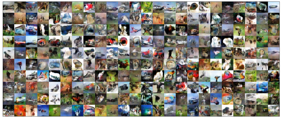
Figure 7: Samples generated from the best WGAN-GP model trained with SGDA.

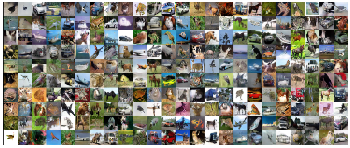
Figure 8: Samples generated from the best WGAN-GP model trained with clipped-SGDA.

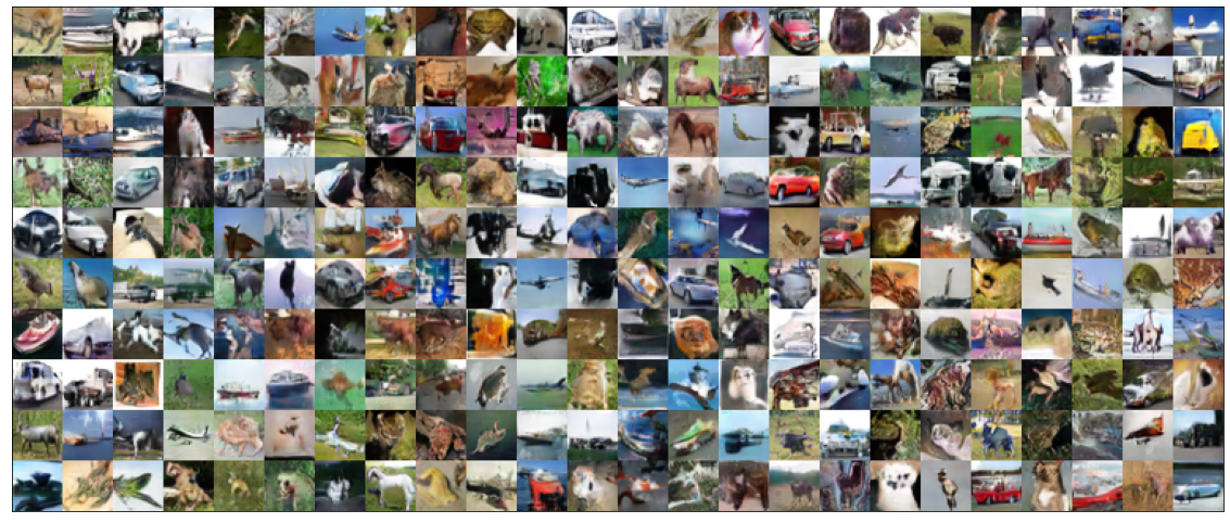
Figure 9: Samples generated from the best WGAN-GP model trained with clipped-SEG.

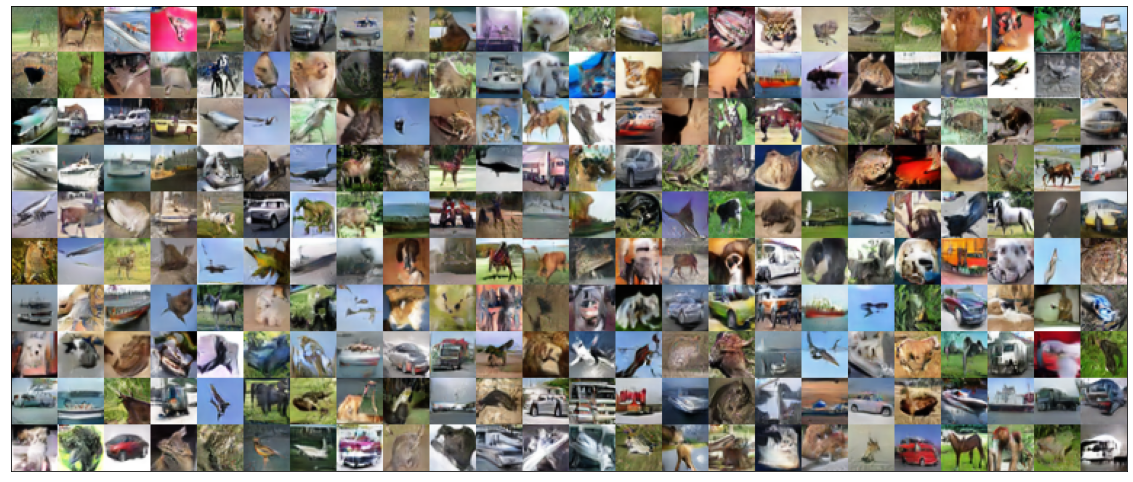
Figure 10: Samples generated from the best WGAN-GP model trained with clipped-SGDA (coordinate clipping).

Generator
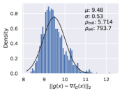
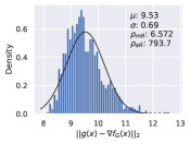
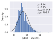
Discriminator

Figure 12: Evolution of gradient noise histograms for the best WGAN-GP model trained with SGDA.

Generator
Discriminator
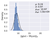
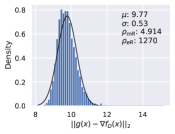
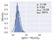
	20000 steps	40000 steps	80000 steps	100000 steps

Figure 13: Evolution of gradient noise histograms for the best WGAN-GP model trained with clipped-SGDA.

Generator
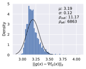
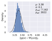
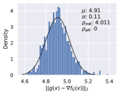
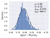
Discriminator
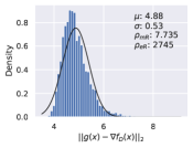
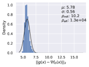
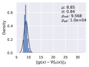
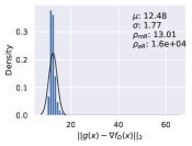
	20000 steps	40000 steps	80000 steps	100000 steps

Figure 14: Evolution of gradient noise histograms for the best WGAN-GP model trained with clipped-SEG.

Generator
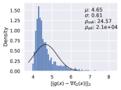
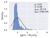
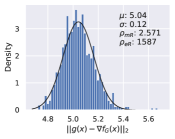
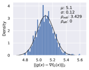
Discriminator
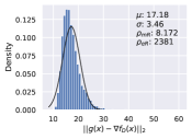
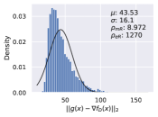
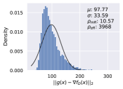
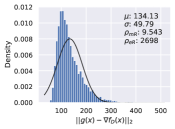
	20000 steps	40000 steps	80000 steps	100000 steps

Figure 15: Evolution of gradient noise histograms for the best WGAN-GP model trained with clipped-SGDA (cordinate clipping).

All of the hyperparameter sweeps performed for SGDA, clipped-SGDA, clipped-SEG, clipped-SGDA (coordinate), and clipped-SEG (coordinate), as well as the associated best FID score obtained within the first 35k training steps, can be found in Tables 3, 7, 5, 7, and 7 respectively. Bold rows denote the hyperparameters that were trained for the full 100k steps and are henceforth referred to as the “best models”. For each of the methods tested, additional samples for the best models trained can be found in Figures 7, 8, 9, 10, & 11. We also plot the evolution of the gradient noise histograms in Figures 12, 13, 14, 15, & 16. We emphasize that our goal is not to get the best possible FID score (e.g. are often able to obtain marginally better FIDs by training for longer), but rather to compare the systematic differences in performance between the various unclipped and clipped methods. Therefore, log-space hyperparameter sweeps are appropriate for our experiments and we do not tune further.

E.2 StyleGAN2

We train on FFHQ downsampled to $128\times 128$ pixels, and use the recommended StyleGAN2 hyperparameter configuration for this resolution: batch size $=32$, $\gamma=0.1024$, map depth $=2$, and channel multiplier $=16384$. For both SGDA and clipped-SGDA, we sweep over a (roughly) log-scale of learning rates and clipping values; a summary of the hyperparmaters and best FID scores obtained Table 9 and Table 9 respectively.

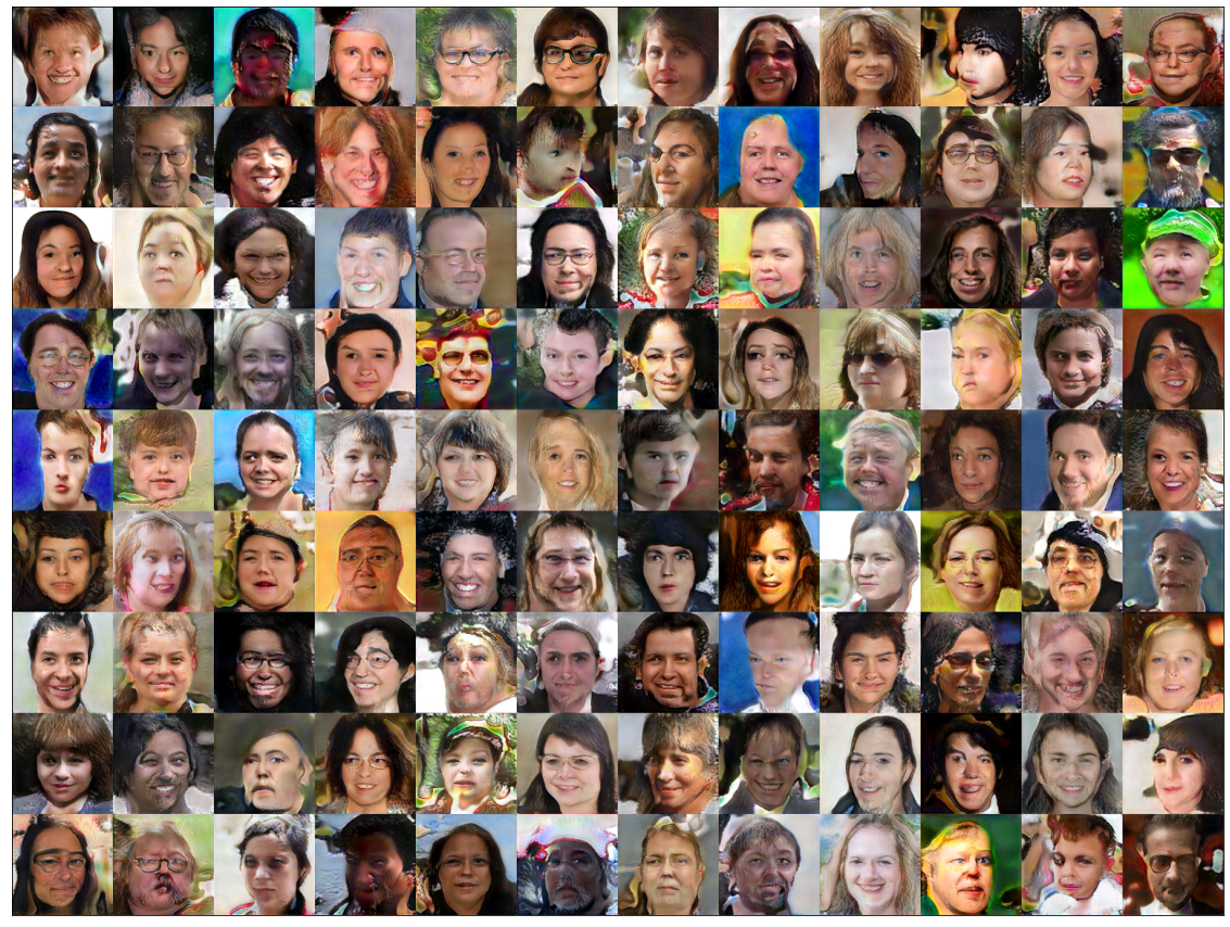
(a) Additional samples generated from our best model trained with clipped-SGDA (lr=0.35, clip=0.0025).

(b) Additional samples generated from several different SGDA trained models, all of which failed to generate meaningful features. Each row corresponds to a model trained with different learning rates.

Figure 18: More StyleGAN2 samples.

Based on the results in Table 9, the best hyperparameters are lr=$0.35$ and clip=$0.0025$ which we then used to train our “best model”. We trained for longer, and decayed the learning rate twice (by a factor of $\times 10$) when the FID plateaued or worsened. The best schedule we found was to scale the learning rate by $\times 0.1$ after 6000 kimgs (thousands of real images shown to the discriminator), by another $\times 0.1$ after 3600 kimgs, and then train until the FID begins increasing (for another 8000 kimgs) – for a total of 17600 kimgs. We did not explore different scale factors or other schedules (such as cosine annealing). Additional samples for this model can be found in Figure 18(a).

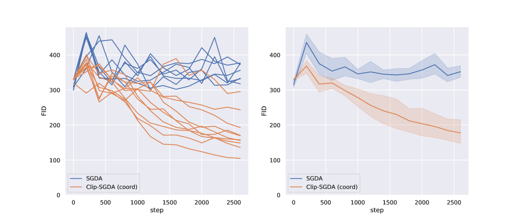
Figure 17: FID curves when training StyleGAN2 for 2600 kimgs (thousands of images seen by the discriminator) with SGDA and clipped-SGDA (coordinate), corresponding to the hyperparameters in Tables 9 & 9 respectively. The left figure is the individual runs for each choice of hyperparameters, and the right is the mean and $95\%$ confidence interval of these runs. Every SGDA-trained model for the wide range of learning rates we tried failed to improve the FID, while models trained with clipped-SGDA (with appropriately set hyperparameters) are generally able to learn some meaningful features and improve the FID.

In general, we observe that every SGDA-trained model for the wide range of learning rates we tested failed to improve the FID, while models trained with clipped-SGDA (with appropriately set hyperparameters) are generally able to learn some meaningful features and improve the FID. We show this behaviour in Figure 17 – the FID scores for SGDA-trained models fluctuate around $320$ and only generate noise such as the samples shown in Figure 18(b), which is in contrast to models trained with clipped-SGDA. Note that the range of the hyperparameter sweep is fairly narrow and favourable for clipped-SGDA, while being quite wide for SGDA. The purpose for these parameter ranges is not to directly compare the parameter sweeps (which would unfairly favour clipped-SGDA), but to show that in general SGDA fails, while clipped-SGDA is capable of learning.

Table 2: SGDA hyperparameter sweep, and the best FID score obtained in 35k training steps.

G-LR	D-LR	FID
6e-06	6e-06	233.3
2e-05	2e-05	177.2
2e-05	4e-05	183.4
2e-05	8e-05	187.3
0.0002	0.0002	85.6
0.0002	0.0004	82.8
0.0002	0.0008	NaN
0.002	0.002	NaN
0.02	0.02	NaN
0.2	0.2	NaN

Table 3: SEG hyperparameter sweep, and the best FID score obtained in 35k training steps.

G-LR	D-LR	FID
6e-06	6e-06	236.1
2e-05	2e-05	208.6
2e-05	4e-05	213.7
4e-05	4e-05	176.5
4e-05	0.0001	NaN
0.0002	0.0002	NaN
0.0002	0.0004	NaN
0.0002	0.0008	NaN
0.002	0.002	NaN
0.02	0.02	NaN
0.2	0.2	NaN
2	2	NaN

Table 4: clipped-SGDA (norm) hyperparameter sweep, and the best FID score obtained in 35k training steps.

G-LR	D-LR	G-clip	D-clip	FID
0.002	0.002	0.1	0.1	257.6
0.002	0.002	1	1	121.6
0.002	0.002	10	10	145.4
0.02	0.02	0.1	0.1	115.4
0.02	0.02	1	1	141.8
0.02	0.02	10	10	27.4
0.2	0.2	0.1	0.1	133.0
0.2	0.2	1	1	26.3
2	2	0.1	0.1	26.1

Table 5: clipped-SEG (norm) hyperparameter sweep, and the best FID score obtained in 35k training steps (17.5k parameter updates).

G-LR	D-LR	G-clip	D-clip	FID
0.002	0.002	0.1	0.1	232.5
0.002	0.002	1	1	150.5
0.002	0.002	10	10	192.7
0.02	0.02	0.1	0.1	161.0
0.02	0.02	1	1	160.3
0.02	0.02	10	10	39.3
0.2	0.2	0.1	0.1	160.0
0.2	0.2	1	1	36.3
2	2	0.1	0.1	37.7

Table 6: clipped-SGDA (coordinate) hyperparameter sweep, and the best FID score obtained in 35k training steps.

G-LR	D-LR	G-clip	D-clip	FID
0.0002	0.0002	0.001	0.001	292.2
0.0002	0.0002	0.01	0.01	108.6
0.0002	0.0002	0.1	0.1	91.5
0.002	0.002	0.001	0.001	76.5
0.002	0.002	0.01	0.01	43.5
0.002	0.002	0.1	0.1	45.1
0.02	0.02	0.001	0.001	37.3
0.02	0.02	0.01	0.01	26.7
0.02	0.02	0.1	0.1	34.7

Table 7: clipped-SEG (coordinate) hyperparameter sweep, and the best FID score obtained in 35k training steps (17.5k parameter updates).

G-LR	D-LR	G-clip	D-clip	FID
0.0002	0.0002	0.001	0.001	298.7
0.0002	0.0002	0.01	0.01	146.5
0.0002	0.0002	0.1	0.1	158.4
0.002	0.002	0.001	0.001	112.8
0.002	0.002	0.01	0.01	52.7
0.002	0.002	0.1	0.1	66.5
0.02	0.02	0.001	0.001	43.5
0.02	0.02	0.01	0.01	36.2
0.02	0.02	0.1	0.1	75.3

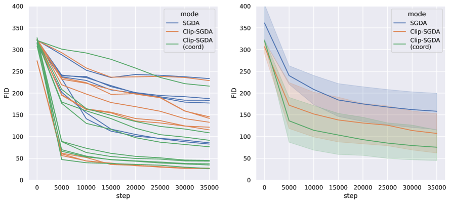
Figure 5: FID curves when training WGAN-GP for 35k steps with SGDA, clipped-SGDA (norm), and clipped-SGDA (coordinate), corresponding to the hyperparameters in Tables 3, 5 & 7 respectively. The left figure is the individual runs for each choice of hyperparameters, and the right is the mean and $95\%$ confidence interval of these runs. Note that 4 of 10 runs diverged (NaN loss) for SGDA, which is not reflected in the mean FID for the right figure beyond the first step.

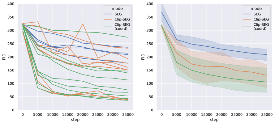
Figure 6: FID curves when training WGAN-GP for 35k steps with SEG, clipped-SEG (norm), and clipped-SEG (coordinate), corresponding to the hyperparameters in Tables 3, 5 & 7 respectively. The left figure is the individual runs for each choice of hyperparameters, and the right is the mean and $95\%$ confidence interval of these runs. Note that 8 of 12 runs diverged (NaN loss) for SEG, which is not reflected in the mean FID for the right figure beyond the first step.

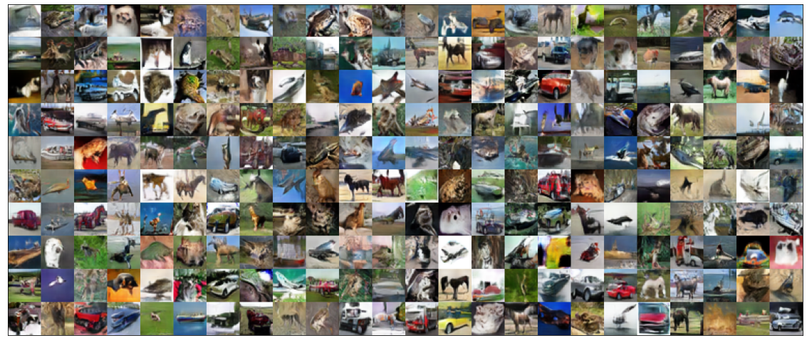
Figure 11: Samples generated from the best WGAN-GP model trained with clipped-SEG (coordinate clipping).

Generator
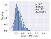
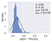
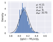
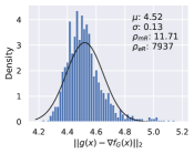
Discriminator
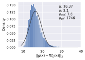
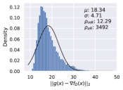
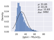
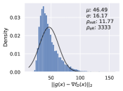
	20000 steps	40000 steps	80000 steps	100000 steps

Figure 16: Evolution of gradient noise histograms for the best WGAN-GP model trained with clipped-SEG (cordinate clipping).

Table 8: StyleGAN2 SGDA hyperparameter sweep, and the best FID score obtained in 2600 kimgs.

G-LR	D-LR	FID
0.003	0.003	319.7
0.0075	0.0075	318.5
0.01	0.01	317.7
0.035	0.035	301.9
0.05	0.05	300.3
0.075	0.075	299.6
0.1	0.1	308.5
0.35	0.35	342.6
0.5	0.5	346.6

Table 9: StyleGAN2 clipped-SGDA (coordinate) hyperparameter sweep, and the best FID score obtained in 2600 kimgs. Bold row denotes the best run which was trained to convergence.

G-LR	D-LR	G-clip	D-clip	FID
0.2	0.2	0.001	0.001	243.5
0.3	0.3	0.001	0.001	169.5
0.35	0.35	0.0005	0.0005	192.9
0.35	0.35	0.001	0.001	148.6
0.35	0.35	0.0025	0.0025	104.9
0.35	0.35	0.005	0.005	149.1
0.35	0.5	0.01	0.01	170.6
0.4	0.4	0.001	0.001	155.8
0.5	0.5	0.0001	0.0001	289.8
0.5	0.5	0.001	0.001	136.1

References

- Abernethy et al. [2019] J. Abernethy, K. A. Lai, and A. Wibisono. Last-iterate convergence rates for min-max optimization. arXiv preprint arXiv:1906.02027, 2019.
- Bauschke et al. [2021] H. H. Bauschke, W. M. Moursi, and X. Wang. Generalized monotone operators and their averaged resolvents. Mathematical Programming, 189(1):55–74, 2021.
- Bennett [1962] G. Bennett. Probability inequalities for the sum of independent random variables. Journal of the American Statistical Association, 57(297):33–45, 1962.
- Beznosikov et al. [2020] A. Beznosikov, V. Samokhin, and A. Gasnikov. Distributed saddle-point problems: Lower bounds, optimal and robust algorithms. arXiv preprint arXiv:2010.13112, 2020.
- Beznosikov et al. [2022] A. Beznosikov, E. Gorbunov, H. Berard, and N. Loizou. Stochastic gradient descent-ascent: Unified theory and new efficient methods. arXiv preprint arXiv:2202.07262, 2022.
- Böhm [2022] A. Böhm. Solving nonconvex-nonconcave min-max problems exhibiting weak minty solutions. arXiv preprint arXiv:2201.12247, 2022.
- Bose et al. [2020] J. Bose, G. Gidel, H. Berard, A. Cianflone, P. Vincent, S. Lacoste-Julien, and W. Hamilton. Adversarial example games. In H. Larochelle, M. Ranzato, R. Hadsell, M. F. Balcan, and H. Lin, editors, Advances in Neural Information Processing Systems, volume 33, pages 8921–8934. Curran Associates, Inc., 2020.
- Brock et al. [2019] A. Brock, J. Donahue, and K. Simonyan. Large scale GAN training for high fidelity natural image synthesis. In International Conference on Learning Representations, 2019. URL https://openreview.net/forum?id=B1xsqj09Fm.
- Cutkosky and Mehta [2021] A. Cutkosky and H. Mehta. High-probability bounds for non-convex stochastic optimization with heavy tails. Advances in Neural Information Processing Systems, 34, 2021.
- Daskalakis et al. [2021] C. Daskalakis, S. Skoulakis, and M. Zampetakis. The complexity of constrained min-max optimization. In Proceedings of the 53rd Annual ACM SIGACT Symposium on Theory of Computing, pages 1466–1478, 2021.
- Davis et al. [2021] D. Davis, D. Drusvyatskiy, L. Xiao, and J. Zhang. From low probability to high confidence in stochastic convex optimization. Journal of Machine Learning Research, 22(49):1–38, 2021.
- Dem’yanov and Pevnyi [1972] V. F. Dem’yanov and A. B. Pevnyi. Numerical methods for finding saddle points. USSR Computational Mathematics and Mathematical Physics, 12(5):11–52, 1972.
- Diakonikolas et al. [2021] J. Diakonikolas, C. Daskalakis, and M. Jordan. Efficient methods for structured nonconvex-nonconcave min-max optimization. In International Conference on Artificial Intelligence and Statistics, pages 2746–2754. PMLR, 2021.
- Dzhaparidze and Van Zanten [2001] K. Dzhaparidze and J. Van Zanten. On bernstein-type inequalities for martingales. Stochastic processes and their applications, 93(1):109–117, 2001.
- Freedman et al. [1975] D. A. Freedman et al. On tail probabilities for martingales. the Annals of Probability, 3(1):100–118, 1975.
- Ghadimi and Lan [2012] S. Ghadimi and G. Lan. Optimal stochastic approximation algorithms for strongly convex stochastic composite optimization i: A generic algorithmic framework. SIAM Journal on Optimization, 22(4):1469–1492, 2012.
- Ghadimi and Lan [2013] S. Ghadimi and G. Lan. Stochastic first-and zeroth-order methods for nonconvex stochastic programming. SIAM Journal on Optimization, 23(4):2341–2368, 2013.
- Gidel et al. [2019a] G. Gidel, H. Berard, G. Vignoud, P. Vincent, and S. Lacoste-Julien. A variational inequality perspective on generative adversarial networks. International Conference on Learning Representations, 2019a.
- Gidel et al. [2019b] G. Gidel, R. A. Hemmat, M. Pezeshki, R. Le Priol, G. Huang, S. Lacoste-Julien, and I. Mitliagkas. Negative momentum for improved game dynamics. In The 22nd International Conference on Artificial Intelligence and Statistics. PMLR, 2019b.
- Goodfellow et al. [2014] I. Goodfellow, J. Pouget-Abadie, M. Mirza, B. Xu, D. Warde-Farley, S. Ozair, A. Courville, and Y. Bengio. Generative adversarial nets. In Z. Ghahramani, M. Welling, C. Cortes, N. Lawrence, and K. Q. Weinberger, editors, Advances in Neural Information Processing Systems, volume 27. Curran Associates, Inc., 2014.
- Goodfellow et al. [2016a] I. Goodfellow, Y. Bengio, and A. Courville. Deep Learning. MIT Press, 2016a. http://www.deeplearningbook.org.
- Goodfellow et al. [2016b] I. Goodfellow, Y. Bengio, and A. Courville. Deep learning. MIT press, 2016b.
- Gorbunov et al. [2020] E. Gorbunov, M. Danilova, and A. Gasnikov. Stochastic optimization with heavy-tailed noise via accelerated gradient clipping. Advances in Neural Information Processing Systems, 33:15042–15053, 2020.
- Gorbunov et al. [2021] E. Gorbunov, M. Danilova, I. Shibaev, P. Dvurechensky, and A. Gasnikov. Near-optimal high probability complexity bounds for non-smooth stochastic optimization with heavy-tailed noise. arXiv preprint arXiv:2106.05958, 2021.
- Gorbunov et al. [2022a] E. Gorbunov, H. Berard, G. Gidel, and N. Loizou. Stochastic extragradient: General analysis and improved rates. In International Conference on Artificial Intelligence and Statistics, pages 7865–7901. PMLR, 2022a.
- Gorbunov et al. [2022b] E. Gorbunov, N. Loizou, and G. Gidel. Extragradient method: O (1/k) last-iterate convergence for monotone variational inequalities and connections with cocoercivity. In International Conference on Artificial Intelligence and Statistics, pages 366–402. PMLR, 2022b.
- Gulrajani et al. [2017] I. Gulrajani, F. Ahmed, M. Arjovsky, V. Dumoulin, and A. C. Courville. Improved training of wasserstein gans. Advances in neural information processing systems, 30, 2017.
- Harker and Pang [1990] P. T. Harker and J.-S. Pang. Finite-dimensional variational inequality and nonlinear complementarity problems: a survey of theory, algorithms and applications. Mathematical programming, 48(1):161–220, 1990.
- Hazan et al. [2015] E. Hazan, K. Levy, and S. Shalev-Shwartz. Beyond convexity: Stochastic quasi-convex optimization. In Advances in Neural Information Processing Systems, pages 1594–1602, 2015.
- Heusel et al. [2017] M. Heusel, H. Ramsauer, T. Unterthiner, B. Nessler, and S. Hochreiter. Gans trained by a two time-scale update rule converge to a local nash equilibrium. Advances in neural information processing systems, 30, 2017.
- Hsieh et al. [2019] Y.-G. Hsieh, F. Iutzeler, J. Malick, and P. Mertikopoulos. On the convergence of single-call stochastic extra-gradient methods. In H. Wallach, H. Larochelle, A. Beygelzimer, F. d'Alché-Buc, E. Fox, and R. Garnett, editors, Advances in Neural Information Processing Systems, volume 32. Curran Associates, Inc., 2019.
- Hsieh et al. [2020] Y.-G. Hsieh, F. Iutzeler, J. Malick, and P. Mertikopoulos. Explore aggressively, update conservatively: Stochastic extragradient methods with variable stepsize scaling. Advances in Neural Information Processing Systems, 33, 2020.
- Jelassi et al. [2022] S. Jelassi, A. Mensch, G. Gidel, and Y. Li. Adam is no better than normalized SGD: Dissecting how adaptivity improves GAN performance, 2022. URL https://openreview.net/forum?id=D9SuLzhgK9.
- Jordanova and Petkova [2017] P. K. Jordanova and M. P. Petkova. Measuring heavy-tailedness of distributions. In AIP Conference Proceedings, volume 1910, page 060002. AIP Publishing LLC, 2017.
- Juditsky et al. [2011a] A. Juditsky, A. Nemirovski, and C. Tauvel. Solving variational inequalities with stochastic mirror-prox algorithm. Stochastic Systems, 1(1):17–58, 2011a.
- Juditsky et al. [2011b] A. Juditsky, A. Nemirovski, et al. First order methods for nonsmooth convex large-scale optimization, i: general purpose methods. Optimization for Machine Learning, pages 121–148, 2011b.
- Karras et al. [2019] T. Karras, S. Laine, and T. Aila. A style-based generator architecture for generative adversarial networks. In Proceedings of the IEEE/CVF conference on computer vision and pattern recognition, pages 4401–4410, 2019.
- Karras et al. [2020] T. Karras, S. Laine, M. Aittala, J. Hellsten, J. Lehtinen, and T. Aila. Analyzing and improving the image quality of stylegan. In Proceedings of the IEEE/CVF conference on computer vision and pattern recognition, pages 8110–8119, 2020.
- Kingma and Ba [2014] D. P. Kingma and J. Ba. Adam: A method for stochastic optimization. arXiv preprint arXiv:1412.6980, 2014.
- Korpelevich [1976] G. M. Korpelevich. The extragradient method for finding saddle points and other problems. Matecon, 12:747–756, 1976.
- Krizhevsky et al. [2009] A. Krizhevsky, G. Hinton, et al. Learning multiple layers of features from tiny images. 2009.
- Lee and Kim [2021] S. Lee and D. Kim. Fast extra gradient methods for smooth structured nonconvex-nonconcave minimax problems. Advances in Neural Information Processing Systems, 34, 2021.
- Loizou et al. [2020] N. Loizou, H. Berard, A. Jolicoeur-Martineau, P. Vincent, S. Lacoste-Julien, and I. Mitliagkas. Stochastic hamiltonian gradient methods for smooth games. In International Conference on Machine Learning, pages 6370–6381. PMLR, 2020.
- Loizou et al. [2021] N. Loizou, H. Berard, G. Gidel, I. Mitliagkas, and S. Lacoste-Julien. Stochastic gradient descent-ascent and consensus optimization for smooth games: Convergence analysis under expected co-coercivity. Advances in Neural Information Processing Systems, 34, 2021.
- Mai and Johansson [2021] V. V. Mai and M. Johansson. Stability and convergence of stochastic gradient clipping: Beyond lipschitz continuity and smoothness. arXiv preprint arXiv:2102.06489, 2021.
- Mertikopoulos and Zhou [2019] P. Mertikopoulos and Z. Zhou. Learning in games with continuous action sets and unknown payoff functions. Mathematical Programming, 173(1):465–507, 2019.
- Mishchenko et al. [2020] K. Mishchenko, D. Kovalev, E. Shulgin, P. Richtarik, and Y. Malitsky. Revisiting stochastic extragradient. In S. Chiappa and R. Calandra, editors, Proceedings of the Twenty Third International Conference on Artificial Intelligence and Statistics, volume 108 of Proceedings of Machine Learning Research, pages 4573–4582. PMLR, 26–28 Aug 2020.
- Miyato et al. [2018] T. Miyato, T. Kataoka, M. Koyama, and Y. Yoshida. Spectral normalization for generative adversarial networks. In ICLR, 2018.
- Nazin et al. [2019] A. V. Nazin, A. Nemirovsky, A. B. Tsybakov, and A. Juditsky. Algorithms of robust stochastic optimization based on mirror descent method. Automation and Remote Control, 80(9):1607–1627, 2019.
- Nemirovski et al. [2009] A. Nemirovski, A. Juditsky, G. Lan, and A. Shapiro. Robust stochastic approximation approach to stochastic programming. SIAM Journal on optimization, 19(4):1574–1609, 2009.
- Nesterov [2007] Y. Nesterov. Dual extrapolation and its applications to solving variational inequalities and related problems. Mathematical Programming, 109(2):319–344, 2007.
- Pascanu et al. [2013] R. Pascanu, T. Mikolov, and Y. Bengio. On the difficulty of training recurrent neural networks. In International conference on machine learning, pages 1310–1318, 2013.
- Robbins and Monro [1951] H. Robbins and S. Monro. A stochastic approximation method. The annals of mathematical statistics, pages 400–407, 1951.
- Ryu and Yin [2021] E. K. Ryu and W. Yin. Large-scale convex optimization via monotone operators, 2021.
- Sauer et al. [2022] A. Sauer, K. Schwarz, and A. Geiger. Stylegan-xl: Scaling stylegan to large diverse datasets. volume abs/2201.00273, 2022. URL https://arxiv.org/abs/2201.00273.
- Song et al. [2020] C. Song, Z. Zhou, Y. Zhou, Y. Jiang, and Y. Ma. Optimistic dual extrapolation for coherent non-monotone variational inequalities. Advances in Neural Information Processing Systems, 33:14303–14314, 2020.
- Tran et al. [2019] N.-T. Tran, V.-H. Tran, B.-N. Nguyen, L. Yang, and N.-M. M. Cheung. Self-supervised gan: Analysis and improvement with multi-class minimax game. Advances in Neural Information Processing Systems, 32, 2019.
- Vezhnevets et al. [2017] A. S. Vezhnevets, S. Osindero, T. Schaul, N. Heess, M. Jaderberg, D. Silver, and K. Kavukcuoglu. Feudal networks for hierarchical reinforcement learning. In International Conference on Machine Learning, pages 3540–3549. PMLR, 2017.
- Wayne and Abbott [2014] G. Wayne and L. Abbott. Hierarchical control using networks trained with higher-level forward models. Neural computation, 26(10):2163–2193, 2014.
- Zhang et al. [2020a] J. Zhang, T. He, S. Sra, and A. Jadbabaie. Why gradient clipping accelerates training: A theoretical justification for adaptivity. In International Conference on Learning Representations, 2020a. URL https://openreview.net/forum?id=BJgnXpVYwS.
- Zhang et al. [2020b] J. Zhang, S. P. Karimireddy, A. Veit, S. Kim, S. J. Reddi, S. Kumar, and S. Sra. Why are adaptive methods good for attention models? Advances in Neural Information Processing Systems, 33, 2020b.