Policy Gradient Algorithms
with Monte-Carlo Tree Search
for Non-Markov Decision Processes

Abstract

Policy gradient (PG) is a reinforcement learning (RL) approach that optimizes a parameterized policy model for an expected return using gradient ascent. Given a well-parameterized policy model, such as a neural network model, with appropriate initial parameters, the PG algorithms work well even when environment does not have the Markov property. Otherwise, they can be trapped on a plateau or suffer from peakiness effects. As another successful RL approach, algorithms based on Monte-Carlo Tree Search (MCTS), which include AlphaZero, have obtained groundbreaking results especially on the board game playing domain. They are also suitable to be applied to non-Markov decision processes. However, since the standard MCTS does not have the ability to learn state representation, the size of the tree-search space can be too large to search. In this work, we examine a mixture policy of PG and MCTS in order to complement each other’s difficulties and take advantage of them. We derive conditions for asymptotic convergence with results of a two-timescale stochastic approximation and propose an algorithm that satisfies these conditions. The effectivity of the proposed methods is verified through numerical experiments on non-Markov decision processes.

Keywords Reinforcement learning  $\cdot$ Policy gradient  $\cdot$ Monte-Carlo tree search  $\cdot$ Non-Markov decision making

1 Introduction

Reinforcement learning (RL) attempts to learn a policy model so as to maximize the average of cumulative rewards Sutton and Barto (2018). Policy gradient (PG) algorithms are based on the gradient ascent in policy parameter space Gullapalli (1990); Williams (1992); Baxter and Bartlett (2001). They can benefit much from recent advances in neural network models and have been applied in various challenging domains, such as robotics Peters and Schaal (2008), image captioning Rennie et al. (2017), document summarization Paulus et al. (2018), and speech recognition Zhou et al. (2018). Another successful RL would be the algorithms based on Monte Carlo Tree Search (MCTS), which utilize Monte Carlo sampling and optimistic tree search that balances exploration and exploitation Kocsis and Szepesvári (2006); Coulom (2006); Browne et al. (2012). In particular, MCTS-based RL algorithms combined with deep learning, such as AlphaZero Silver et al. (2017a, b) and MuZero Schrittwieser et al. (2020), have represented a significant improvement over previous algorithms and obtained groundbreaking results especially on the board game playing domain Silver et al. (2016).

Ordinary RL uses a fundamental assumption that the environment has Markov property, i.e., the reward process and system dynamics of the underlying process are Markovian. More specifically, they depend only on the current state (and action); in other words, given the current state, they are independent of the past states. This enables computationally effective dynamic programming techniques to learn policy models Puterman (1994); Bertsekas (1995). However, in many real-world RL tasks, it is difficult to determine in advance a good state set or space that satisfies the Markov property Yu et al. (2011); Friedrich et al. (2011); Berg et al. (2012); Clarke et al. (2015); Rennie et al. (2017); Paulus et al. (2018); Zhou et al. (2018); You et al. (2018).

There are at least two typical scenarios in which the Markov property are violated. The first is related to the observation. If the observations are limited and partial, the dynamics and rewards are not Markovian and need to be modeled with functions of the past observation sequence or functions of a latent state. Typical examples are dialog systems Young et al. (2013) and robot navigation Berg et al. (2012). The other case is when only the reward function is not Markovian. Generation task, such as text Yu et al. (2017) and molecular graph You et al. (2018), is an typical example since generated objects are usually evaluated not only on a local but also on a global perspective, such as ad quality score in the domain of text generation for search engine advertising Kamigaito et al. (2021). The former scenario is often formulated as a partially observable Markov decision process (POMDP) Kaelbling et al. (1996); Sondik (1971), while the latter is a a decision process with non-Markovian reward (NMRDP) Bacchus et al. (1996). The stochastic process that includes both is called a non-Markovian decision process (NMDP) or history-based decision process (HDP) Whitehead and Lin (1995); Bacchus et al. (1997); Majeed and Hutter (2018), which is the focus of this paper.

It is noteworthy that algorithms based on PG or MCTS could work even if a task is a HDP Kimura et al. (1997); Aberdeen (2003); Rennie et al. (2017); Browne et al. (2012) since they do not heavily depend on the Bellman optimality equation under the Markov assumption unlike Q learning and deep Q network (DQN) Sutton and Barto (2018). Among them, PG algorithms can directly take advantage of the use of function approximators like neural networks. However, it has long been known that PGs are occasionally trapped on a plateau and are slow to learn Kakade (2002); Morimura et al. (2014); Ciosek and Whiteson (2020). In addition, PGs could suffer from the peakiness issue, where the initially most probable actions will gain probability mass, even if they are not the most rewarding Choshen et al. (2020); Kiegeland and Kreutzer (2021). On the other hand, MCTS-based algorithms can maintain a proper balance between the exploration and exploitation, and thus is probable to converge to the global optimal Kocsis and Szepesvári (2006); Lattimore and Szepesvári (2020); Świechowski et al. (2021). Compared to PG, however, MCTS, except for the AlphaZero-based approach Silver et al. (2017a), usually lacks the ability to learn state representation because it creates a node for each history. Thus, the size of the tree-search space can be too large to search.

Based on the above, we believe that PG and MCTS can complement each other’s difficulties and their combination is promising way to solving problems on HDPs. Specifically, even when PG is suffering from plateaus or the peakiness issue, MCTS is likely to be able to continue to improve its policy because its exploration-exploitation and training strategies are fundamentally different from PG’s. PG with an appropriately parameterized model would be able to cover the inefficiency in the state representation of MCTS. It is also generally known that a combination of models can have a positive effect Kuncheva (2014). In this work, we investigate an approach using a mixture of PG and MCTS policies, with the aim of taking advantages of the characteristics of both the PG and MCTS frameworks (Figure 1). We call this approach a policy gradient guided by MCTS (PG-MCTS). We derive conditions for asymptotic convergence and find that simply mixing policies will not work in terms of asymptotic convergence. We propose an algorithm that satisfies the conditions for convergence.

The organization and the contributions of this paper are summarized as follows. Section 2 provides background information for RL of HDPs, PG, and MCTS. In Section 3, we propose an approach of PG-MCTS and then show its convergence conditions by using results of a two-timescale stochastic approximation. We also show an implementation that satisfies the convergence conditions and converges to a reasonable solution by reformulating and modifying the MCTS update and by revising the PG update. They are our main contribution. In Section 4, we will review some related work. Finally, the effectivity of combination of PG and MCTS is demonstrated through numerical experiments in Section 5, and Section 6 concludes the paper.

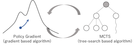
Figure 1: The concept of the proposed approach (PG-MCTS). The PG and MCTS have different properties and the PG-MCTS takes advantage of those strong points and mitigates the bad ones.

2 Preliminaries

We define our problem setting of RL in a history-based decision process (HDP) in Section 2.1. PG and MCTS algorithms are briefly reviewed in Section 2.2 and 2.3, respectively.

2.1 Problem Setting of RL in HDP

While problems of RL are usually formulated on a Markov decision process (MDP) for ease of learning Sutton and Barto (2018), as described in Section 1, it is difficult to define Markovian states in many real-world tasks. Here, we consider a discrete-time episodic HDP Whitehead and Lin (1995); Majeed and Hutter (2018) as a general decision process without assuming the Markovian property. It is defined by a tuple $\mathsf{HDP}\triangleq\{\mathcal{O},\mathcal{A},{T_{\rm max}},p_{\textrm{ini}},p_{\textrm{o}},f_{\textrm{r}}\}$, which are as follows:

• $\mathcal{O}$ is a finite set of observations.

• $\mathcal{A}$ is a finite set of actions.

• ${T_{\rm max}}$ is the length of each episode.

• $p_{\textrm{ini}}:\mathcal{O}\rightarrow[0,1]$ is a probability function of the initial observation, $p_{\textrm{ini}}(o_{0})\triangleq\Pr(o_{0})$ .

• $p_{\textrm{o}}:\mathcal{O}\times\mathcal{H}_{t}\times\mathcal{A}\rightarrow[0,1]$ is a history-dependent observation probability function at each time step $t\in\{0,1\dots,{T_{\rm max}}\}$,

  $$p_{\textrm{o}}(o_{t+1}|h_{t},a_{t}) \triangleq\Pr(O_{t+1}\!\!=\!o_{t+1}\,|\,H_{t}\!=\!h_{t},A_{t}\!=\!a_{t}),\ \ \ \forall(o_{t+1},h_{t},a_{t})\in\mathcal{O}\times\mathcal{H}_{t}\times\mathcal{A},$$

  where $h_{t}\!\triangleq\![o_{0},a_{0},\dots,o_{t-1},a_{t-1},o_{t}]\!=\![h_{t-1},a_{t-1},o_{t}]$ is a history up to a time step $t$, and $\mathcal{H}_{t}\triangleq(\mathcal{O}\times\mathcal{A})^{t}\times\mathcal{O}$ is a set of histories at a time step $t$. We notate the total history set $\mathcal{H}\triangleq\bigcup_{t=0}^{{T_{\rm max}}}\mathcal{H}_{t}$ and the history transition probability function $p_{\textrm{h}}:\mathcal{H}_{t+1}\times\mathcal{H}_{t}\times\mathcal{A}\rightarrow[0,1]$ at $t\in\{0,\dots,{T_{\rm max}}\!-1\}$ such as

  $$p_{\textrm{h}}(h_{t+1}\!=\![h_{t},a_{t},o_{t+1}]\,|\,h_{t},a_{t})\triangleq p_{\textrm{o}}(o_{t+1}|h_{t},a_{t}).$$

• $f_{\textrm{r}}:\mathcal{H}\times\mathcal{A}\rightarrow[-{R_{\rm max}},{R_{\rm max}}]$ is a history-dependent bounded reward function, which defines an immediate reward $r_{t}=f_{\textrm{r}}(h_{t},a_{t})$ at time step $t\in\{0,\dots,{T_{\rm max}}\}$.

Here we bring in the length ${T_{\rm max}}$ mainly to simplify the presentation of the paper. If we set ${T_{\rm max}}$ to a sufficiently large value and assume that once an agent reaches a terminal state, it stays there until ${T_{\rm max}}$, the effect of ${T_{\rm max}}$ can be practically ignored.

A learning agent chooses an action according to an policy model $\pi:\mathcal{A}\times\mathcal{H}\rightarrow[0,1]$, which is a conditional action probability function $\pi(a|h_{t})\triangleq\Pr(a\,|\,h_{t},\pi)$ at each time step $t$ in an episode. Without loss of generality, we assume that the agent can take any action $a\in\mathcal{A}$ in any $h_{t}\in\mathcal{H}_{t}$ at any $t\in\{0,\dots,{T_{\rm max}}\}$.

The agent learns the policy model $\pi$ by experiencing episodes repeatedly. The objective function that the agent seeks to maximize is the expected return

$$\Upsilon(\pi)\triangleq\mathbb{E}^{\pi}[G_{0}],$$ (1)

where we use this notation $\mathbb{E}^{\pi}[\,\cdot\,]\triangleq\mathbb{E}[\,\cdot\,|\,\mathsf{HDP},\pi]$ and $G_{t}$ is a random variable of the return at time step $t\in\{0,\dots,{T_{\rm max}}\}$,

$$G_{t}\triangleq\sum_{k=t}^{T_{\rm max}}R_{k}=\sum_{k=t}^{T_{\rm max}}f_{\textrm{r}}(H_{k},A_{k}).$$

Although the discount factor $\gamma\in[0,1]$ is often used, as in $G_{t}=\sum_{k=t}^{{T_{\rm max}}}\gamma^{k-t}R_{k}$, we omit it for simplicity, since all our results are immediately applicable to the case with $\gamma<1$.

As in normal RL settings, we assume that $p_{\textrm{ini}}$, $p_{\textrm{o}}$, and $f_{\textrm{r}}$ are usually unknown to the agent. However, even when they are known to the agent, it is almost impossible to analytically evaluate Eq. ​(1) or solve RL problems in HDPs. This is because there is a combinatorially large number of histories and thus the history space cannot be fully searched. So an approximation approach like RL is necessary in HDPs.

2.2 Policy gradient

We assume that the policy model $\pi^{\theta}$ to be optimized by PG algorithms is parameterized by a parameter $\theta\in\mathbb{R}^{d}$ and $\pi^{\theta}$ is always differentiable with respect to $\theta$. Typical instance of $\pi^{\theta}$ is a neural network for sequence learning, such as a recurrent neural network (RNN) Hochreiter and Schmidhuber (1997); Wierstra et al. (2010); Rennie et al. (2017) and Transformer Vaswani et al. (2017); Chen et al. (2021). The PG algorithms are based on the gradient method of the following update rule with a small learning rate $\alpha\geq 0$,

$$\theta :=\theta+\alpha\nabla_{\theta\hskip 0.28453pt}\Upsilon(\pi^{\theta}),$$

where $:=$ is the right-to-left substitution operator and $\nabla_{\theta\hskip 0.28453pt}\Upsilon(\pi^{\theta})\triangleq[\partial\Upsilon(\pi^{\theta})/\partial{\theta_{1}},...,\partial\Upsilon(\pi^{\theta})/\partial{\theta_{d}}]^{\!\top}$ is the gradient of $\Upsilon(\pi^{\theta})$ with respect to $\theta$. Because the analytical evaluation of $\nabla_{\theta\hskip 0.28453pt}\Upsilon(\pi^{\theta})$ is generally intractable, a PG method, called REINFORCE Williams (1992), updates $\theta_{n}$ after every episode $n$ of experience $[o_{0},a_{0},r_{0},\dots,o_{T_{\rm max}},a_{T_{\rm max}},r_{T_{\rm max}}]$ according to a stochastic gradient method as follows:

$$\theta_{n+1}=\theta_{n}+\alpha_{n}\sum_{t=0}^{T_{\rm max}}\nabla_{\theta\hskip 0.28453pt}\log\pi^{\theta_{n}}(a_{t}|h_{t})\,(g_{t}-b(h_{t})),$$ (2)

since the gradient $\nabla_{\theta\hskip 0.28453pt}\Upsilon(\pi^{\theta})$ is written as

$$\nabla_{\theta\hskip 0.28453pt}\Upsilon(\pi^{\theta})=\mathbb{E}^{\pi^{\theta}}\!\!\left[\,\sum_{t=0}^{T_{\rm max}}\nabla_{\theta\hskip 0.28453pt}\log\pi^{\theta}(A_{t},H_{t})\,(G_{t}-b(H_{t}))\right]\!\!,$$

where $g_{t}$ is an is an observation of the return $G_{t}$ and $b:\mathcal{H}\rightarrow\mathbb{R}$ is an arbitrary baseline function. This is used for reducing the variance of the stochastic gradient, which is the second term on the right side of Eq. ​(2), and dose not induce any bias to the gradient as long as it does not depend on the action because of

$$\mathbb{E}^{\pi^{\theta}} [\nabla_{\theta\hskip 0.28453pt}\log\pi^{\theta}(A_{t}|H_{t})\,b(H_{t})\,|\,H_{t}\!=\!h]=b(h)\sum_{a}\nabla_{\theta\hskip 0.28453pt}\pi^{\theta}(a|h)=b(h)\nabla_{\theta\hskip 0.28453pt}\sum_{a}\pi^{\theta}(a|h)=b(h)\nabla_{\theta\hskip 0.28453pt}1=0.$$

Here, we notate $\sum_{a\in\mathcal{A}}$ as $\sum_{a}$ for simplicity.

2.3 Monte Carlo tree search

Monte Carlo tree search (MCTS) algorithms are originally heuristic search methods for decision processes to identify the best action in a given situation Kocsis and Szepesvári (2006); Coulom (2006); Browne et al. (2012). Even time they run an episode from the given situation, they gain knowledge and store it in a tree by expanding the tree and updating statistics in nodes of the tree. In single-agent learning in a stochastic system dynamics, the tree usually has two kinds of nodes, a history node and a history-action node, alternating in the depth direction. If a tree-search agent is at a non-leaf history node in the tree, the transition to its child node, which is a history-action node, is determined according to the action selected by a policy of the tree-search agent. The transition from a history-action node to its child node, the history node, follows the history transition probability $p_{\textrm{h}}$.

Each history-action node holds a return estimate $q$ and the number of visits $m$ as the statistics. Here, we notate those statistics in each history-action node $(h,a)$ with a tabular representation, as $q(h,a)$ and $m(h,a)$, for simplicity. The tree policy at a history node $h$ decides an action using the statistics of its child nodes, such as

$$\arg\max_{a}\left\{q(h,a)+C\sqrt{\frac{\log(\sum_{b}m(h,b))}{m(h,a)}}\right\}$$ (3)

where $C\geq 0$ is a hyper-parameter to control the balance between exploration and development. This formula is called upper confidence bounds applied for trees (UCT) Kocsis and Szepesvári (2006) and is one of the most commonly used implementations in the MCTS.

Each iteration of the MCTS consists of four consecutive phases: $\rm(\hskip 1.79993pti\hskip 1.79993pt)$ selection of child nodes from the root to a leaf node in the tree, $\rm(\hskip 0.80002ptii\hskip 0.80002pt)$ tree expansion by new child nodes that are initialized as $m\!:=\!1,\ q\!:=\!0$, $\rm(iii)$ simulation from one of the new nodes according to a default policy to compute the return, and $\rm(iv)$ back-propagation of the feedback to the tree. Note that $\rm(\hskip 0.80002ptii\hskip 0.80002pt)$ and $\rm(iii)$ are skipped if the leaf node reached is a terminal node, and $\rm(iii)$ is the “Monte Carlo” part of the algorithm. The default policy, which is used in $\rm(iii)$, is usually a uniform random policy.

In the back-propagation phase of $\rm(iv)$, the statistics of the node visited at each depth $t$ of iteration $n\in\{1,2,\dots\}$ are updated as follows:

$$\begin{cases}\displaystyle m_{n+1}(h_{t},a_{t})&\!\!\!\!\displaystyle=m_{n}(h_{t},a_{t})+1,\\ q_{n+1}(h_{t},a_{t})&\!\!\!\!\displaystyle=q_{n}(h_{t},a_{t})+\frac{1}{m_{n}(h_{t},a_{t})}(g_{t}-q_{n}(h_{t},a_{t})),\end{cases}$$ (4)

where $g_{t}$ is an observation of the return $G_{t}$. In addition to the above, many other update rules have been proposed, such as the TD ($\lambda$) learning type Browne et al. (2012); Vodopivec et al. (2017).

3 Policy gradient guided by MCTS

We first show our general approach of mixture policies of PG and MCTS, called PG guided by MCTS (PG-MCTS), in Section 3.1. The convergence analysis of the PG-MCTS is provided in Section 3.2. In Section 3.3, we propose an implementation that satisfies the convergence conditions and converges to a reasonable solution.

3.1 General approach

Our approach to combining PG and MCTS is simple, basically just randomly selecting a policy of either PG or MCTS at each time step. For this purpose, we will use the MCTS in a slightly lazy way.

At every decision-making or time step in actual interaction with the environment, the MCTS typically runs a number of episodes with a simulator, rebuild (or update) a tree, and select an action. However, just like the PG, our MCTS-based policy, which we simply call a MCTS policy, does not use a simulator and just uses the tree that has already been built. This MCTS policy consists of two types of sub-policies, which are tree-search and default policies. The tree-search policy is used at $h$ if the tree holds a node $h$ and its child nodes $(h,a)$. Otherwise, the default policy is used. After experiencing an episode, the MCTS policy is updated according to the back-propagation procedure of the MCTS (e.g. Eq. (4)). Thus we will have at most $|\mathcal{H}_{0}|$ trees, which is equal to the size of observation set $|\mathcal{O}|$. While this type of MCTS may not be irregular, we will refer to it as “lazy MCTS” to distinguish it from the standard MCTS. For now, let the policy model of the lazy MCTS be a stochastic policy $\pi^{\omega}$, which we call the MCTS policy, and let its parameter be $\omega$. Specific implementations, including update rules, are described in Section 3.3.

Now both of the parameterized policy $\pi^{\theta}$, which we call the PG policy, and the MCTS policy $\pi^{\omega}$ can make online decision-making without a simulator. So, we consider the following mixture of policies $\pi^{\theta}$ and $\pi^{\omega}$:

$$\pi^{\theta\!,\omega}(a|h)\triangleq(1-\lambda(h))\pi^{\theta}(a|h)+\lambda(h)\pi^{\omega}(a|h),$$ (5)

where $\lambda$ is a mixing probability. The $\lambda$ may be constant or depend on an observation $o$, history $h$, and parameters $\theta$, $\omega$. The parameters $\theta$ and $\omega$ are updated with modified methods of the PG and MCTS, respectively, which are proposed in Section 3.3 by using the results in Section 3.2.

3.2 Convergence analysis

We present the convergence conditions of the PG-MCTS on a few settings of the mixing probability $\lambda_{n}$ in Eq. ​(5). Proofs are shown in Appendix.

As we will validate our assumptions in the next section, but for now, we assume that the update rules of the PG and MCTS policies can be rewritten in the following form:

$$\theta_{n+1} =\theta_{n}+\alpha_{n}[\,k(\theta_{n},\omega_{n})+M^{(1)}_{n+1}+\epsilon^{(1)}_{n}],$$ (6)

$$\omega_{n+1} =\omega_{n}+\eta_{n}[\,l(\theta_{n},\omega_{n})+M^{(2)}_{n+1}+\epsilon^{(2)}_{n}],$$ (7)

where $h:\mathbb{R}^{d}\times\mathbb{R}^{e}\!\rightarrow\mathbb{R}^{d}$ and $g:\mathbb{R}^{d}\times\mathbb{R}^{e}\!\rightarrow\mathbb{R}^{e}$ are the expected update functions, $M^{(1)}\!\in\mathbb{R}^{d}$ and $M^{(2)}\!\in\mathbb{R}^{e}$ are noise terms, and $\epsilon^{(1)}\!\in\mathbb{R}^{d}$ and $\epsilon^{(2)}\!\in\mathbb{R}^{e}$ are bias terms.

We make the following assumptions about the noise and bias terms, which are common in the stochastic approximation Borkar (2008).

Assumption 1.

The stochastic series $\{M^{(i)}_{n}\}$ for $i=1,2$ is a martingale difference sequence, i.e., with respect to the increasing $\sigma$-fields,

$$\mathcal{F}_{n}\triangleq\sigma(\theta_{m},\omega_{m},M^{(1)}_{m},M^{(2)}_{m},m\leq n),$$

for some constant $K>0$, the following holds,

$$\mathbb{E}[\,M^{(i)}_{n+1}\,|\,\mathcal{F}_{n}] =0,\ \ \forall n\in\{1,2,\dots\},$$

$$\mathbb{E}[\,\lVert M^{(i)}_{n+1}\rVert^{2}\,|\,\mathcal{F}_{n}] \leq K(1+\lVert\theta_{n}\rVert^{2}+\lVert\omega_{n}\rVert^{2}),\ \ \forall n\in\{1,2,\dots\}.$$

Assumption 2.

The bias $\{\epsilon^{(i)}_{n}\}$ for $i=1,2$ is a deterministic or random bounded sequence which is $o(1)$, i.e.,

$$\lim_{n\rightarrow\infty}\epsilon^{(i)}_{n}=0.$$

For our analysis, we use the ordinary differential equation (ODE) approach for the stochastic approximation Bertsekas and Tsitsiklis (1996); Borkar (2008). The limiting ODEs that Eqs. ​(6) and (7) might be expected to track asymptotically is, for $\tau\geq 0$,

$$\dot{\theta}(\tau) =k(\theta(\tau),\omega(\tau)),$$ (8)

$$\dot{\omega}(\tau) =l(\theta(\tau),\omega(\tau)).$$ (9)

We also make the assumption about the expected update functions $k$ and $l$.

Assumption 3.

The functions $k$ and $l$ be Lipschitz continuous maps, i.e., for some constants $L_{1},L_{2}<\infty$,

$$\lVert k(\theta,\omega)-k(\theta^{\prime},\omega^{\prime})\rVert \leq L_{1}\lVert[\theta,\omega]-[\theta^{\prime},\omega]\rVert,\,\forall(\theta,\omega,\theta^{\prime},\omega^{\prime}),$$

$$\lVert l(\theta,\omega)-l(\theta^{\prime},\omega^{\prime})\rVert \leq L_{2}\lVert[\theta,\omega]-[\theta^{\prime},\omega]\rVert,\,\forall(\theta,\omega,\theta^{\prime},\omega^{\prime}).$$

Assumption 4.

The ODE of Eq. ​(9) has a globally asymptotically stable equilibrium $\varphi(\theta)$, where $\varphi:\mathbb{R}^{d}\rightarrow\mathbb{R}^{e}$ is a Lipschitz map.

Assumption 5.

$\sup_{n}(\lVert\theta_{n}\rVert+\lVert\omega_{n}\rVert)<\infty$.

We first show show the convergence analysis result for the case of that the mixing probability $\lambda$ is a constant or a fixed function such as $\lambda:\mathcal{H}\rightarrow[0,1]$.

Proposition 1.

Assume Assumptions 1–5 hold. Let the mixing probability function $\lambda:\mathcal{H}\rightarrow[0,1]$ be invariant to the number of episodes $n$, and the learning rates $\alpha_{n}$ and $\eta_{n}$ satisfying

$$\left\{\begin{array}[]{l}\displaystyle\ \lim_{N\rightarrow\infty}\sum_{n=0}^{N}\alpha_{n}=\lim_{N\rightarrow\infty}\sum_{n=0}^{N}\eta_{n}=\infty,\\[14.22636pt] \displaystyle\ \lim_{N\rightarrow\infty}\sum_{n=0}^{N}\big{(}\alpha_{n}^{2}+\eta_{n}^{2}\big{)}<\infty,\\[14.22636pt] \displaystyle\ \lim_{N\rightarrow\infty}\frac{\alpha_{N}}{\eta_{N}}=0.\end{array}\right.$$ (13)

Then, almost surely, the sequence $\{(\theta_{n},\omega_{n})\}$ generated by Eqs. ​(6) and (7) converges to a compact connected internally chain transitive invariant set of Eqs. ​(8) and (9).

The above results indicate how the learning rates $\alpha_{n}$ and $\eta_{n}$ should be set for the convergence. Since $\eta_{n}$ in the MCTS policy is basically proportional to $\frac{1}{n}$, an obvious choice of $\alpha_{n}$ will be $\frac{1}{1+n\log n}$. Note that, if a deterministic policy such as UCT (Eq. ​(3)) is used, $k$ and $l$ will not be the Lipschitz maps and thus the above convergence results cannot be applied. Thus, we will use the softmax function Sutton and Barto (2018) in the implementation in Section 3.3.

The invariant condition of $\lambda$ can be relaxed.

Proposition 2.

Let $\lambda_{\theta_{n}}:\mathcal{H}\rightarrow[0,1]$ be a function parameterized by a part of $\theta$ and a Lipschitz continuous map with respect to $\theta$. Assume that all the conditions of Proposition 1 are satisfied expect for $\lambda$. Still, the consequence of Proposition 1 holds.

Finally, we consider the case that $\lambda_{n}$ is a decreasing function of the number of episodes $n$, where the MCTS policy $\pi^{\omega}$ is just used for guiding the PG. The goal in this case will be to obtain a parameterized policy $\pi^{\theta}$ that demonstrates good performance by itself. In the case of $\lambda_{n}$ decreasing, the convergence condition can be significantly relaxed as follows.

Proposition 3.

Assume Assumptions 1 and 2 only for $i=1$ hold, $k$ is Lipschitz continuous map, and $\sup_{n}(\lVert\theta_{n}\rVert)<\infty$ holds. Let the mixing probability $\lambda_{n}$ be $o(1)$ and satisfy $0\leq\lambda_{n}\leq 1-\varepsilon$ for all $n$ and a constant $\varepsilon>0$, and the learning rate of the PG policy satisfy

$$\lim_{N\rightarrow\infty}\sum_{n=0}^{N}\alpha_{n}=\infty,\quad\lim_{N\rightarrow\infty}\sum_{n=0}^{N}\alpha_{n}^{2}<\infty.$$

Then, almost surely, the sequence $\{\theta_{n}\}$ generated by Eqs. ​(6) and (7) converges to a compact connected internally chain transitive invariant set of the ODE, $\dot{\theta}(\tau)=\nabla_{\theta\hskip 0.28453pt}\Upsilon(\pi^{\theta{(\tau)}})$.

This proposition shows that, unlike the previous cases, the convergence property is guaranteed even if a deterministic policy like UCT is used for the MCTS policy.

3.3 Implementation

We present an implementation of the PG-MCTS that satisfies the convergence conditions and converges to a reasonable solution.

First, we consider revising the update of $\pi^{\theta}$. Since the goal is to maximize the expected return of Eq. ​(1), the following update at each episode $n$ will be appropriate, instead of the ordinary PG update of Eq. ​(2):

$$\theta_{n+1} =\theta_{n}+\alpha_{n}\sum_{t=0}^{T_{\rm max}}\nabla_{\theta\hskip 0.28453pt}\log\pi^{\theta_{n},\omega_{n}}(a_{t}|h_{t})(g_{t}-b(h_{t}))$$

$$=\theta_{n}+\alpha_{n}\sum_{t=0}^{T_{\rm max}}\rho_{t}\nabla_{\theta\hskip 0.28453pt}\log\pi^{\theta_{n}}(a_{t}|h_{t})(g_{t}-b(h_{t})),$$ (14)

where we assume $\pi^{\theta_{n},\omega_{n}}$ is the behavior policy of the episode $n$. The $\rho_{t}$ is a scaled probability ratio or a kind of the importance weight Sutton and Barto (2018),

$$\rho_{t}\triangleq\frac{(1-\lambda(h_{t}))\pi^{\theta}(a_{t}|h_{t})}{\pi^{\theta\!,\omega}(a_{t}|h_{t})}.$$ (15)

From Proposition 2, it does not violate the conditions of convergence if the mixture probability function $\lambda$ is trained with the PG update rather than treating $\lambda$ as given in advance. In that case, we assume the function $\lambda_{\theta}$ is parameterized by some parameter in $\theta$. Then, the update rule is derived as

$$\theta_{n+1}=\theta_{n}+\alpha_{n}\sum_{t=0}^{T_{\rm max}}\bigg{(}\rho_{t}\nabla_{\theta\hskip 0.28453pt}\log\pi^{\theta_{n}}+\frac{(\pi^{\omega_{n}}-\pi^{\theta_{n}})}{\pi^{\theta_{n},\omega_{n}}}\nabla_{\theta\hskip 0.28453pt}\lambda_{\theta_{n}}\bigg{)}(g_{t}-b(h_{t})).$$ (16)

From here on, we will only consider the case where the mixing probability $\lambda$ is constant, but the results introduced hare will be straightforwardly applied to other settings of $\lambda$.

Next, we consider an implementation of the MCTS policy $\pi^{\omega}$. The update rule of the MCTS is seemingly different the general update rule of the stochastic approximation, Eq. ​(7). In particular, the learning rate in the MCTS update of Eq. ​(4) could be different among the nodes. Especially, the values of an unexpanded node $(h_{t},a_{t})$ will not be updated. On the other hand, the update of the stochastic approximation assume that there exists a global learning rate $\eta_{n}$ (see Eq. (7)). Furthermore, Assumption 5 for convergence requires that the parameters are always bounded, but the number of visits $m$ diverges. To fill the gap, we introduce a tree-inclusion probability and reformulate the MCTS update by replacing $m(h,a)$ with $u\!:\!\mathcal{H}\!\times\!\mathcal{A}\rightarrow[0,1]$ so that $m(h,a)\!=\!1/u(h,a)$. That is, the parameter of the MCTS policy $\pi^{\omega}$ is $\omega\triangleq\{u,q\}$. The original MCTS update of Eq. ​(4) can be rewritten as follows, with the learning rate $\eta_{n}=1/n$ and the initialization $u\!:=\!1$, $q\!:=\!0$,

$$\begin{cases}\displaystyle u_{n+1}(h_{t},a_{t})&\!\!\!\!\displaystyle=u_{n}(h_{t},a_{t})+\eta_{n}\kappa_{n,t}\frac{-u_{n}(h_{t},a_{t})}{u_{n}(h_{t},a_{t})+1},\\[5.69054pt] q_{n+1}(h_{t},a_{t})&\!\!\!\!\displaystyle=q_{n}(h_{t},a_{t})+\eta_{n}\kappa_{n,t}(g_{t}-q_{n}(h_{t},a_{t})),\end{cases}$$ (17)

where $\kappa_{n,t}$ is the following and can be regarded as an adjustment term for the learning rate per node,

$$\kappa_{n,t} \triangleq p_{n,t}\,\frac{u_{n}(h_{t},a_{t})}{\eta_{n}},$$

and $p_{n,t}$ is the following tree-inclusion probability,

$$p_{n,t} \triangleq\begin{cases}1,&\ \textrm{if\ }t=0,\\ \min\!\left(\frac{1}{u_{n}(h_{t-1},a_{t-1})}-1,1\right),&\ \textrm{otherwise}.\end{cases}$$ (18)

In this update, if $u_{n}(h_{t-1},a_{t-1})=1$, the tree-inclusion probability $p_{n,t}$ is zero and thus the values of $(h_{t},a_{t})$ are not updated. This corresponds to the case where a node $(h_{t},a_{t})$ is not expanded. If $u_{n}(h_{t-1},a_{t-1})\leq 0.5$, the values of a node $(h_{t},a_{t})$ are updated with probability $1$. The equivalence of the original MCTS update and Eq. (17) is shown in Appendix.

We next investigate Assumption 3 about Lipschitz continuity of the expected update functions $k$ and $l$. The PG update of Eq. (14) is based on the gradient ascent and thus the expected update functions $k$ with an ordinary implementation will satisfy Lipschitz continuity. However, the MCTS update of Eq. (17) does not allow $l$ to have Lipschitz continuity since $\kappa_{n,t}$ diverges as $z_{n}\rightarrow 0$. This problem can be solved by modifying $\kappa_{n,t}$ with a large value $M>0$ as follows:

$$\bar{\kappa}_{n,t} \triangleq\min(\kappa_{n,t},M).$$ (19)

Theorem 1.

Let the PG-MCTS update the parameterized policy $\pi^{\theta}$ by Eq. ​(14) and the MCTS policy $\pi^{\omega}$ by Eq. ​(17) with replacing $\kappa$ by $\bar{\kappa}$ of Eq. ​(19), and the learning rates satisfy the conditions of Eq. ​(13). Also let $\pi^{\theta}$ be defined on a compact parameter space and have always bounded first and second partial derivatives, and $\pi^{\omega}$ be a softmax policy with hyper parameters $\beta\geq 0$ and $C\geq 0$,

$$\pi^{\omega}\!(a|h)\propto\exp\!\!\left(\!\!\beta\Big{\{}q(h,\!a)+C\!\sqrt{u(h,\!a)\log\!\sum_{b}\frac{1}{u(h,\!b)}}\Big{\}}\!\!\right)\!\!.$$ (20)

Then, $\lim_{n\rightarrow\infty}\nabla_{\theta\hskip 0.28453pt}\Upsilon(\pi^{\theta_{n},\omega_{n}})=0$ holds.

Finally, we propose a heuristic to avoid a vanishing gradient problem of the PG update of Eq. (14). By the definition of $\rho_{t}$ in Eq. ​(15), if $\pi^{\theta}$ and $\pi^{\theta\!,\omega}$ are significantly different, $\rho_{t}$ can be close to zero and thus the stochastic gradient at time $t$ can be vanished. In order to avoid this problem, we modify $\rho_{t}$ to $\underline{\rho}_{t}$ as, with $\upsilon\in[0,1]$,

$$\underline{\rho}_{t}\triangleq\max(\upsilon,\rho_{t}).$$ (21)

When $\upsilon_{n}=o(1)$ holds, the convergence property in Theorem 1 is preserved because $\upsilon_{n}$ is absorbed into $\epsilon_{n}$ in Eq. ​(6). Also note that $\rho_{t}$ is upper bounded by 1. Thus there is no need to care about $\rho_{t}$ taking a large value.

The entire procedure of this PG-MCTS implementation is shown in Algorithm 1.

Algorithm 1 A PG-MCTS implementation

  given:

    - an initialized PG policy $\pi^{\theta}(a|h)$

    - an initialized MCTS policy $\pi^{\omega}(a|h)$, e.g., Eq. ​(20)

    - hyper-parameters for the PG and MCTS policies

    - a mixing probability function $\lambda(h)$

  while within computational budget do

     // interaction with environment $\mathsf{HDP}$

     observe an initial observation $h_{0}\sim p_{\textrm{ini}}$

     empty a memory $\mathcal{M}$ and store $h_{0}$ in $\mathcal{M}$

     for $t=0$ to ${T_{\rm max}}$ do

        choose a policy $\pi\in\{\pi^{\theta},\pi^{\omega}\}$, using $\lambda(h_{t})$ (see Eq. ​(5))

        choose and execute an action $a_{t}\sim\pi(\,\cdot\,|h_{t})$

        observe a reward $r_{t}:=f_{\textrm{r}}(h_{t},a_{t})$

        observe a new history $h_{t+1}\sim p_{\textrm{h}}(\,\cdot\,|h_{t},a_{t})$

        store $r_{t}$ and $h_{t+1}$ in the memory $\mathcal{M}$

     end for

     // update of policies $\pi^{\theta}$ and $\pi^{\omega}$ with $M$

     update $\pi^{\theta}$ by the PG update of Eq. ​(14) or (16) with (21)

     update $\pi^{\omega}$ by the MCTS update of Eq. ​(17) with (19)

     compute the return $g_{t},\ \forall t\in\{0,\dots,{T_{\rm max}}\}$

  end while

  return  the learned policy $\pi^{\theta\!,\omega}\triangleq\lambda\pi^{\theta}+(1-\lambda)\pi^{\omega}$

4 Related work

There are a lot of studies that integrate MCTS and RL algorithms Guo et al. (2014); Vodopivec et al. (2017); Silver et al. (2017a); Jiang et al. (2018); Efroni et al. (2019); Ma et al. (2019); Schrittwieser et al. (2020); Grill et al. (2020); Dam et al. (2021). Most of them are based on the standard MCTS setting and propose to use value-based RL Vodopivec et al. (2017); Jiang et al. (2018); Efroni et al. (2019) or supervised learning Guo et al. (2014); Silver et al. (2017a); Anthony et al. (2017); Schrittwieser et al. (2020); Grill et al. (2020); Dam et al. (2021), where deep neural networks are trained from targets generated by the MCTS iterations. The latter approach is also known as expert iteration Anthony et al. (2017). The most well-known algorithms of adopting this approach will be AlphaZero Silver et al. (2017a, b) and MuZero Schrittwieser et al. (2020). The critical difference between the expert iteration and the PG-MCTS will be the policy updates. While the PG-MCTS is weighting the experiences with the return $g_{t}$ and importance weight $\rho_{t}$ (see Eq. (14)), the standard expert iteration does not, assuming that most instances for policy update are positive examples since they are outputs of the MCTS iterations. Another difference is the type of learning: the expert iteration will be classified as model-based RL or assuming environment is known, while the PG-MCTS is model-free.

There are several studies of combining MCTS with PG Guo et al. (2016); Anthony et al. (2019); Soemers et al. (2019); Dieb et al. (2020). Guo et al. (2016) uses PG to design reward-bonus functions to improve the performance of MCTS. Anthony et al. (2019) uses PG for updating local policies and investigates planning without an explicit tree search. Dieb et al. (2020) uses PG in the tree expansion phase to choose a promising child node to be created, assuming a situation where the number of actions is huge. On the other hand, Soemers et al. (2019) runs MCTS to compute a value function that PG uses.

For RL in a HDP or NMDP, there are two major directions. The first one assumes the existence of latent dynamics and consider the identification of the dynamics Thiébaux et al. (2006); Poupart and Vlassis (2008); Silver and Veness (2010); Singh et al. (2012); Doshi-Velez et al. (2015); Brafman and Giacomo (2019). The most well known mathematical model for this purpose would be a POMDP Kaelbling et al. (1998). Doshi-Velez et al. (2015) identifies an environment as a POMDP with Bayesian non-parametric methods and then compute a policy by solving the POMDP. The other direction is to use a function approximator whose output depends not only on the current observation but also on the past history Loch and Singh (1998); Hernandez-Gardiol and Mahadevan (2000); Bakker (2002); Hausknecht and Stone (2015); Rennie et al. (2017). One of the successful approaches uses a neural network for sequence learning as a policy model and optimize it by PG Wierstra et al. (2010); Rennie et al. (2017); Paulus et al. (2018); Kamigaito et al. (2021), as corresponding to the PG policy in our proposed PG-MCTS.

While the proposed implementation of the PG-MCTS integrates basic PG and MCTS algorithms in a well-designed way, there are a lot of studies of enhancing those algorithms, such as stabilization of PG by a conservative update Kakade (2002); Schulman et al. (2015, 2017), the entropy regularization for explicitly controlling the exploration-exploitation trade-off Haarnoja et al. (2017, 2018); Xiao et al. (2019); Grill et al. (2020), and extensions of MCTS to continuous spaces Couëtoux et al. (2011); Mansley et al. (2011); Kim et al. (2020); Mao et al. (2020). Incorporating these technologies, including the expert iteration, into the PG-MCTS is an interesting avenue for future work.

5 Numerical Experiments

We apply the PG-MCTS algorithm to two different tasks in HDPs. The first task is randomly synthesized task, which does not contain domain-specific and is not overly complex structures. Therefore, the task will be useful to investigate basic performance of algorithms. The second task is the long-term dependency T-maze, which is a standard benchmark for learning a deep-memory POMDP Bakker (2002); Wierstra et al. (2010). For reasons of space, details of the experimental setup are given in Appendix.

The goal here is not to find the best model for the above two tasks, but to investigate if/how combining the PG and MCTS by the PG-MCTS is effective. Therefore, the applied algorithms here are simple, not the state-of-the-art algorithms. In this regard, model-based RL including MuZero Schrittwieser et al. (2020) are also out of scope of this work. We used REINFORCE Williams (1992) for the PG and the lazy MCTS for the MCTS, which are introduced in Section 2.2 and 3.1, respectively. Note that REINFORCE, although classic, is still appealing due to its good empirical performance and simplicity Grooten et al. (2022); Zhang et al. (2021) In fact, it and its variants are used in many applications Rennie et al. (2017); Paulus et al. (2018); Chen et al. (2019); Xia et al. (2020); Wang et al. (2021). Thus, we believe that improving REINFORCE itself is still important in the practical implementation of reinforcement learning.

We also applied a simple version of AlphaZero Silver et al. (2017a), which we call a lazy AlphaZero, which is the same adaptation to the online RL setting as the lazy MCTS. A parameterized policy model used as the prior policy in the lazy AlphaZero is updated by online experiences according to likelihood maximization. In addition to the mixture by the proposed PG-MCTS, we also applied a naive mixture algorithm of the PG and MCTS, which follows Eq. ​(5), but the learning process of each policy is identical to the standalone REINFORCE and lazy MCTS. For fair evaluation, we first tuned the hyper-parameters of standalone algorithms and then used them for the PG-MCTS and the naive mixture model (See Appendix for details).

5.1 Randomly synthesized task

The first task is a non-Markovian task that is randomly synthesized. This is a simple, but very illustrative, a HDP that is modeled to be analogous to generation tasks such as text generation and compound synthesis. There are five observations and ten actions. The observation probability function $p_{\textrm{o}}$ was synthesized so that it depends on the time-step, last observation, and action. The reward function $f_{\textrm{r}}$ was composed to the sum of the per-step sub-reward function $r_{\rm local}$ and the history-based sub-reward function $r_{\rm global}$. The function $r_{\rm global}$ was synthesized by using a Gaussian process, such that the more similar the histories, the closer their rewards tend to be. This reward function $f_{\textrm{r}}$ can be interpreted in the context of text generation as follows: $r_{\rm local}$ represents the quality of local word connections, and $r_{\rm global}$ represents the quality of the generated text. The policy $\pi^{\theta}$ was a softmax and parameterized by using the reward structure. We set ${T_{\rm max}}\!=\!15$. Thus, there are a huge number of variations in the histories ($\sim 10^{25}$).

(a)	(b)

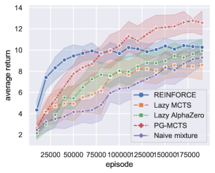
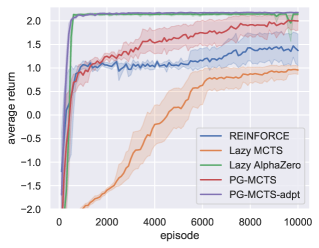
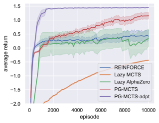
Figure 2: Performance comparison by ten independent runs, where the error bar represents the standard error of the mean: (a) the randomly synthesized task (${T_{\rm max}}=15$). (b) T-maze task; the plot on the left is the result of easy setting (the length of corridor $L=30$ and the initial position $s_{0}=0$). The plot on the right is for more difficult setting, where there exist more sub-optimal policies (the length of corridor $L=100$ and the initial position $s_{0}=50$).

Figure 2 (a) shows the results of ten independent runs. In each run, a HDP environment was generated independently as described above. From the results, we confirmed the significant effect of the proposed PG-MCTS. This indicates that the PG-MCTS has ability to successfully incorporate the advantages of both the PG and MCTS. The subtle performance of the naive mixture indicates that the simple mixing approach of the PG and MCTS policies may not work.

5.2 T-maze task

The second experiment is the non-Markovian T-maze task Bakker (2002); Wierstra et al. (2010) (see Figure 3). It is designed to test an algorithm’s ability to learn associations between events with long time lags. An agent has to remember the observation from the first time step until the episode ends. We use a long short-term memory (LSTM) as a policy model.

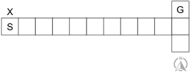
Figure 3: Long-term dependency T-maze task: an agent starts at the position S. Only at the initial time step $t=0$, it can observe a signal ’up’ or ’down’ that indicates it should go north or south at the T-junction in this episode. In this example, the direction is ’up’, the starting position is $s_{0}=0$, and the length of corridor is $L=10$.

Since the original setting with the initial position $s_{0}=0$ is not so difficult, we prepared more difficult setting, where initial position $s_{0}$ is the center of the corridor. In this setting, a policy that chooses the left or right action with probability $0.5$ can be a sub-optimal policy. Note that this is not true in the original setting ($s_{0}=0$) because going left occurs a negative reward.

The results are shown in Figure 2 (b) and indicates the effectivity of the proposed methods, where ’PG-MCTS’ used a fixed the mixing probability $\lambda_{n}$, but ’PG-MCTS-adpt’ learned $\lambda_{\theta}$ with the PG update of (16).

6 Conclusion

In this paper, we focused on history-based decision processes (HDPs) and investigated the approach for mixture policies of the PG and MCTS, called the PG-MCTS approach, in order to take advantages of the characteristics of both the PG and MCTS frameworks. We provided the convergence analysis and then proposed an implementation that converges to a reasonable solution. Through the numerical experiments with the simple HDP tasks, we confirmed significant effect of the proposed approach for the mixture of the PG and MCTS policies. To the best of our knowledge, this is the first study on policy gradient algorithms guided by the MCTS framework with theoretical justification, though there exist studies of MCTS algorithms using the PG to solve partial problems in the MCTS.

In the future work, we will apply our algorithms with the state-of-the-art neural networks for sequence data to more practical and challenging domains, such as text summarization, advertising text generation, and incomplete information games. Further theoretical analysis, especially convergence rate analysis, is necessary to more deeply understand the properties of the PG-MCTS and to improve the algorithms. Also, the analysis of convergence points is interesting because the PG is a local optimization while MCTS is a global optimization method. For example, a guide by MCTS may help PGs get out of a bad local optima as well as a learning plateau. Incorporating the state-of-the-art techniques in the PG and MCTS, such as the entropy regularization and the natural gradient, will be another interesting direction.

Appendix A Proofs

A.1 Preliminaries

We first introduce the basic results on the ordinary differential equation (ODE) based approach of the stochastic approximation Borkar [2008]. We consider the following update rule of $\theta\in\mathbb{R}^{d}$ with an initial value $\theta_{0}\in\mathbb{R}^{d}$ for all $n\in[0,1,\dots]=\mathbb{N}_{\geq 0}$,

$$\theta_{n+1} =\theta_{n}+\alpha_{n}[\,k(\theta_{n})+M_{n+1}+\epsilon_{n}].$$ (22)

To take the ODE approach, we extend the above discrete-time stochastic process of $\theta_{n}$ to a continuous, piecewise-linear counterpart $\bar{\theta}:\mathbb{R}_{\geq 0}\rightarrow\mathbb{R}^{d}$ as follows: Define a time-instant function $t:\mathbb{N}_{\geq 0}\rightarrow\mathbb{R}_{\geq 0}$ such as

$$t(n)\triangleq\begin{cases}0&\textrm{if\ \ }n=0,\\ \sum_{m=0}^{n-1}\alpha_{m}&\textrm{otherwise},\end{cases}$$

and set $\bar{\theta}(t(n))=\theta_{n},\ \forall n\in\mathbb{N}_{\geq 0}$. Then, for any $n\in\mathbb{N}_{\geq 0}$, we derive the following linear interpolation,

$$\bar{\theta}(\tau)\triangleq\theta_{n}+(\theta_{n+1}-\theta_{n})\frac{\tau-t(n)}{t(n+1)-t(n)},\quad\tau\in I_{n},$$ (23)

where $I_{n}\triangleq[t(n),t(n+1)]$. As we will show later, the key result of the ODE approach to the analysis of Eq. (22) is that $\bar{\theta}(\tau)$ asymptotically almost surely approaches the solution set of the following ODE,

$$\dot{\theta}(\tau)=k(\theta(\tau)),\quad\tau\in\mathbb{R}_{\geq 0}.$$ (24)

For the purpose, we need to make the following assumptions.

Assumption 6.

The learning rates $\{\alpha_{n}\}$ are positive scalars satisfying

$$\lim_{N\rightarrow\infty}\sum_{n=0}^{N}\alpha_{n}=\infty,\qquad\lim_{N\rightarrow\infty}\sum_{n=0}^{N}\alpha_{n}^{2}\leq\infty.$$ (25)

Assumption 7.

The function $k:\mathbb{R}^{d}\rightarrow\mathbb{R}^{d}$ is a Lipschitz continuous map, i.e., for some constant $0<L<\infty$,

$$\lVert k(\theta)-k(\theta^{\prime})\rVert\leq L\lVert\theta-\theta^{\prime}\rVert,\qquad\forall(\theta,\theta^{\prime})\in\mathbb{R}^{d}\times\mathbb{R}^{d}.$$

Assumption 8.

The stochastic series $\{M_{n}\}$ is a martingale difference sequence with respect to the increasing family of $\sigma$-fields

$$\mathcal{F}_{n}\triangleq\sigma(\theta_{i},M_{i},\epsilon_{i},i\leq n).$$

That is, the following holds,

$$\mathbb{E}[M_{n+1}\,|\,\mathcal{F}_{n}] =0\quad a.s.,\quad\forall n\geq 0.$$

Furthermore, $M_{n}$ is always square-integrable with

$$\mathbb{E}[\,\lVert M_{n+1}\rVert^{2}\,|\,\mathcal{F}_{n}] =K(1+\lVert\theta_{n}\rVert^{2})\quad\textrm{a.s.},\quad\forall n\geq 0,$$ (26)

for some constant $K\geq 0$.

Assumption 9.

The series of bias $\{\epsilon_{n}\}$ is a deterministic or random bounded sequence which is $o(1)$.

Assumption 10.

The updates of Eq. (22) remain bounded almost surely, i.e.,

$$\sup_{n}\lVert\theta_{n}\rVert<\infty,\quad\textrm{a.s.}$$

Lemma 1.

Assume Assumptions 6–10 hold. Let $\theta^{s}(\tau),\,\tau\geq s\geq 0$, denote the trajectory of Eq. (24) starting at time $s\in\mathbb{R}_{\geq 0}$:

$$\dot{\theta}^{s}(\tau)=k(\theta^{s}(\tau)),\quad\forall\tau\in\mathbb{R}_{\geq s},$$

with $\theta^{s}(s)=\bar{\theta}(s)$. Then, for any $T>0$, the following holds almost surely,

$$\lim_{s\rightarrow\infty}\sup_{\tau\in[s,s+T]}\lVert\bar{\theta}(\tau)-\theta^{s}(\tau)\rVert=0,$$

$$\lim_{s\rightarrow\infty}\sup_{\tau\in[s-T,s]}\lVert\bar{\theta}(\tau)-\theta^{s}(\tau)\rVert=0.$$

Proof:  This lemma is a simple extension of Lemma 1 in Section 2 of Borkar [2008] with a bias term $\epsilon_{n}$, and this proof mostly follows from it. We will only prove the first claim since the same applies to the proof of the second claim.

For $n\in\mathbb{N}_{\geq 0}$ and $m\in\mathbb{N}_{\geq 1}$, by the construction, $\bar{\theta}$ can be written down as follows:

$$\bar{\theta}(t(n+m))=\bar{\theta}(t(n))+\sum_{i=0}^{m-1}\alpha_{n+i}\,k(\bar{\theta}(t(n+i)))+\delta_{n,n+m}.$$ (27)

where

$$\delta_{n,n+m} \triangleq\xi_{n+m}-\xi_{n}+\sum_{i=0}^{m-1}\alpha_{n+i}\,\epsilon_{n+i},$$

$$\xi_{n} \triangleq\begin{cases}0,&\textrm{if\ \ }n=0,\\ \sum_{i=0}^{n-1}\alpha_{i}M_{i+1},&\textrm{if\ \ }n\in\mathbb{N}_{\geq 1}.\end{cases}$$

We will show $\sup_{m\geq 0}\lVert\delta_{n,n+m}\rVert=0$ as $n\rightarrow\infty$. By Assumptions 8 and 10, the series $\{\xi_{n}\}$ is a zero mean, square-integrable martingale with respect to the $\sigma$-fields $\mathcal{F}_{n}$. Furthermore, by Assumptions 6, 8, and 10, we have

$$\sum_{n=0}^{\infty}\mathbb{E}[\,\lVert\xi_{n+1}-\xi_{n}\rVert^{2}\,|\,\mathcal{F}_{n}]=\sum_{n=0}^{\infty}\alpha_{n}^{2}\,\mathbb{E}[\,\lVert M_{n+1}\rVert^{2}\,|\,\mathcal{F}_{n}]<\infty,\quad\textrm{a.s.}$$

From the above and the martingale convergence theorem (Theorem 11 of Appendix in Borkar [2008]), it can be said that $\{\xi_{n}\}$ converges. The third term of $\delta_{n,n+m}$ also converges to zero as $n\rightarrow\infty$ because $\{\epsilon_{n}\}$ is $o(1)$ by Assumption 9. Thus, the following holds,

$$\lim_{n\rightarrow\infty}\lVert\delta_{n,n+m}\rVert=0,\quad\textrm{a.s.}$$ (28)

Next, we will look into $\theta^{s}$. It can be written down as follows:

$$\theta^{t(n)}(t(n+m)) =\bar{\theta}(t(n))+\int_{t(n)}^{t(n+m)}k(\theta^{t(n)}(\tau))d\tau$$

$$=\bar{\theta}(t(n))+\sum_{i=0}^{m-1}\alpha_{n+i}\,k(x^{t(n)}(t(n+i)))+\int_{\tau=t(n)}^{t(n+m)}\!\big{(}k(\theta^{t(n)}(\tau))-k(\theta^{t(n)}(\tilde{\tau}))\big{)}d\tau,$$ (29)

where

$$\tilde{\tau}\triangleq\max\{t(n)\,|\,t(n)\leq\tau,\,n\in\mathbb{N}_{\geq 0}\}.$$

We investigate the integral on the right-hand side in Eq. (29). Let $C_{0}\triangleq\sup_{n}\lVert\theta_{n}\rVert$. Note that $C_{0}<\infty$ a.s. by Assumption 10. By Assumption 7, $\lVert k(\theta)-k(0)\rVert\leq L\lVert\theta\rVert$, and so

$$\lVert k(\theta)\rVert\leq\lVert k(0)\rVert+L\lVert\theta\rVert$$ (30)

Therefore, the following holds, for $\tau\in[s,s+T]$,

$$\lVert\theta^{s}(\tau)\rVert \leq\lVert\bar{\theta}(s)\rVert+\int_{x=s}^{\tau}\big{(}\lVert k(0)\rVert+L\lVert\theta^{s}(x)\rVert\big{)}dx$$

$$\leq C_{0}+\lVert k(0)\rVert T+L\int_{\iota=s}^{\tau}\lVert k(\iota)\rVert d\iota.$$

By Gronwall’s inequality (Lemma 6 of Appendix in Borkar [2008]), we obtain

$$\lVert\theta^{s}(\tau)\rVert\leq\big{(}C_{0}+\lVert k(0)\rVert T)\exp(LT),\quad\forall\tau\in[s,s+T].$$ (31)

Thus, from Eq. (30), we have the following bound,

$$C_{T}\triangleq\lVert k(0)\rVert+L(C_{0}+\lVert k(0)\rVert T)\exp(LT)<\infty,\quad\textrm{a.s.}$$

such that, for all $\tau\in[s,s+T]$,

$$\lVert k(\theta^{s}(\tau))\rVert\leq C_{T}.$$ (32)

Here we assume $T$ is larger than $t(n+m)-t(n)$ without loss of generality. For $i\in\{0,\dots,m-1\}$ and $\tau\in[t(n+i),t(n+i+1)]$, the bound $C_{t}$ gives

$$\lVert\theta^{t(n)}(\tau)-\theta^{t(n)}(t(n+i))\rVert \leq\left\lVert\int_{\iota=t(n+i)}^{\tau}k(\theta^{t(n)}(\iota))d\iota\right\rVert$$

$$\leq C_{T}(\tau-t(n+i))$$

$$\leq C_{T}\alpha_{n+i}.$$

The inequality gives the bound of the integral in Eq. (29) as follows: because

$$\left\lVert\int_{\tau=t(n)}^{t(n+m)}\!\!\big{(}k(\theta^{t(n)}(\tau))-k(\theta^{t(n)}(\tilde{\tau}))\big{)}d\tau\right\rVert \leq\int_{\tau=t(n)}^{t(n+m)}\!\!L\lVert\theta^{t(n)}(\tau)-\theta^{t(n)}(\tilde{\tau})\rVert$$

$$=L\sum_{i=0}^{m-1}\int_{\tau=t(n+i)}^{t(n+i+1)}\lVert\theta^{t(n)}(\tau)-\theta^{t(n)}(t(n+i))\rVert d\tau$$

$$\leq C_{T}L\sum_{i=0}^{m-1}\alpha_{n+i}^{2}$$

Thus, by Assumption 6, we have

$$\lim_{n\rightarrow\infty}\left\lVert\int_{\tau=t(n)}^{t(n+m)}\!\!\big{(}k(\theta^{t(n)}(\tau))-k(\theta^{t(n)}(\tilde{\tau}))\big{)}d\tau\right\rVert\leq C_{T}L\sum_{i=0}^{m-1}\lim_{n\rightarrow\infty}\alpha_{n+i}^{2}=0,\quad\textrm{a.s.}$$ (33)

By subtracting Eq. (27) from Eq. (29) and taking a norm, we have

$$\lVert\bar{\theta}(t(n+m))-\theta^{t(n)}(t(n+m))\rVert\leq L\sum_{i=0}^{m-1}\alpha_{n+i}\lVert\bar{\theta}(t(n+i))-\theta^{t(n)}(t(n+i))\rVert+K_{n,T},$$

where

$$K_{n,T} \triangleq C_{T}L\sum_{i\geq 0}^{\acute{m}_{n,\!T}-1}\alpha_{n+i}^{2}+\lVert\delta_{n,n+\acute{m}_{n,\!T}}\rVert,$$

$$\acute{m}_{n,T} \triangleq\max\{m\,|\,t(n+m)\!-\!t(n)\!\leq\!T,\,m\in\mathbb{N}_{\geq 0}\}.$$

Note that

$$\lim_{n\rightarrow\infty}K_{n,T}=0,\quad\textrm{a.s.}$$ (34)

holds by Eqs. ​(28) and (33). By applying the discrete Gronwall lemma (Lemma 8 of Appendix in Borkar [2008]) to the above inequality, we have

$$\sup_{i\in\{0,\dots,m\}}\lVert\bar{\theta}(t(n+i))-\theta^{t(n)}(t(n+i))\rVert\leq K_{n,T}\exp(LT),\quad\textrm{a.s.}$$ (35)

Let $\tau\in[t(n+i),t(n+i+1)]$ for $0\leq i\leq m-1$. Then we have

$$\bar{\theta}(\tau)=\lambda\theta(t(n+i))+(1-\lambda)\bar{\theta}(t(n+i+1))$$

for some $\lambda\in[0,1]$, and thus the following inequality is obtained,

$$\lVert\bar{\theta}(\tau)-\theta^{t(n)}(\tau)\rVert =\lVert\lambda(\bar{\theta}(t(n+i))-\theta^{t(n)}(\tau))+(1+\lambda)(\bar{\theta}(t(n+i+1))-\theta^{t(n)}(\tau))\rVert$$

$$\leq\lambda\left\lVert\bar{\theta}(t(n+i))-\theta^{t(n)}(t(n+i))-\int_{\iota=t(n+i)}^{\tau}k(\theta^{t(n)})d\iota\right\rVert$$

$$\qquad+(1-\lambda)\left\lVert\bar{\theta}(t(n+i+1))-\theta^{t(n)}(t(n+i+1))+\int_{\iota=\tau}^{t(n+i+1)}k(\theta^{t(n)})d\iota\right\rVert$$

$$\leq\lambda\lVert\bar{\theta}(t(n+i))-\theta^{t(n)}(t(n+i))\rVert+(1-\lambda)\lVert\bar{\theta}(t(n+i+1))-\theta^{t(n)}(t(n+i+1))\rVert$$

$$\qquad+\int_{\iota=t(n+i)}^{t(n+i+1)}\lVert k(\theta^{t(n)}(\iota))\rVert d\iota$$

$$\leq K_{n,T}\exp(LT)+C_{T}\alpha_{n+i},\quad\textrm{a.s.},$$

where the last inequality is derived by using Eqs. ​(35) and (32). The above inequality is easily generalized to, with some constant $C\geq 0$

$$\sup_{\tau\in[s,s+T]}\lVert\bar{\theta}(\tau)-\theta^{t(n)}(\tau)\rVert\leq CK_{\tilde{s},T}\exp(LT)+C_{T}\alpha_{\tilde{s}},$$

where $\tilde{s}\triangleq\max\{t(n)\,|\,t(n)\leq s,\,n\in\mathbb{N}_{\geq 0}\}$. As $s\rightarrow\infty$, we have the first claim in this lemma. ∎

By applying Lemma 1 to Theorem 2 of Section 2 and Theorem 2 of Section 6 in Borkar [2008], we instantly obtain the following lemmas.

Lemma 2.

Assume Assumptions Assumptions 6–10 hold. Then, the sequence $\{\theta_{n}\}$ generated by Eq. (22) almost surely converges to a (possibly sample path dependent) compact connected internally chain transitive invariant set of Eq. (26).

Lemma 3.

Let the sequence $\{(\theta_{n},\omega_{n})\}$ is generated by

$$\theta_{n+1} =\theta_{n}+\alpha_{n}[\,k(\theta_{n},\omega_{n})+M^{(1)}_{n+1}+\epsilon^{(1)}_{n}],$$ (6)

$$\omega_{n+1} =\omega_{n}+\eta_{n}[\,l(\theta_{n},\omega_{n})+M^{(2)}_{n+1}+\epsilon^{(2)}_{n}],$$ (7)

where $k:\mathbb{R}^{d}\times\mathbb{R}^{e}\!\rightarrow\mathbb{R}^{d}$ and $l:\mathbb{R}^{d}\times\mathbb{R}^{e}\!\rightarrow\mathbb{R}^{e}$ are the expected update functions, $M^{(1)}\!\in\mathbb{R}^{d}$ and $M^{(2)}\!\in\mathbb{R}^{e}$ are noise terms, and $\epsilon^{(1)}\!\in\mathbb{R}^{d}$ and $\epsilon^{(2)}\!\in\mathbb{R}^{e}$ are bias terms. Also, let the learning rates $\alpha_{n}$ and $\eta_{n}$ of Eqs. ​(6) and (7) satisfying

$$\left\{\begin{array}[]{l}\displaystyle\ \lim_{N\rightarrow\infty}\sum_{n=0}^{N}\alpha_{n}=\lim_{N\rightarrow\infty}\sum_{n=0}^{N}\eta_{n}=\infty,\\[14.22636pt] \displaystyle\ \lim_{N\rightarrow\infty}\sum_{n=0}^{N}\big{(}\alpha_{n}^{2}+\eta_{n}^{2}\big{)}<\infty,\\[14.22636pt] \displaystyle\ \lim_{N\rightarrow\infty}\frac{\alpha_{N}}{\eta_{N}}=0.\end{array}\right.$$ (39)

Assume Assumptions Assumptions 1–5 hold. Then, the sequence $\{(\theta_{n},\omega_{n})\}$ almost surely converges to a (possibly sample path dependent) compact connected internally chain transitive invariant set $A$ of the following ODEs

$$\dot{\theta}(\tau) =k(\theta(\tau),\omega(\tau)),$$ (8)

$$\dot{\omega}(\tau) =l(\theta(\tau),\omega(\tau)).$$ (9)

Any pair $(\theta,\omega)\in A$ has the relation $\omega=\varphi(\theta)$, where $\varphi(\theta)$ is defined in Assumption 4 and denotes the globally asymptotically stable equilibrium of the ODE (9) of $\omega$ given $\theta$.

A.2 Propositions 1 and 2

By applying Lemma 3 to the update rule of the proposed PG-MCTS algorithm (Eqs. ​(6) and (7)), we immediately obtain Propositions 1 and 2.

Proposition 1.

Assume Assumptions 1–5 hold. Let the mixing probability function $\lambda_{n}:\mathcal{H}\rightarrow[0,1]$ be invariant to the number of episodes $n$ and the learning rates $\alpha_{n}$ and $\eta_{n}$ satisfying

$$\left\{\begin{array}[]{l}\displaystyle\ \lim_{N\rightarrow\infty}\sum_{n=0}^{N}\alpha_{n}=\lim_{N\rightarrow\infty}\sum_{n=0}^{N}\eta_{n}=\infty,\\[14.22636pt] \displaystyle\ \lim_{N\rightarrow\infty}\sum_{n=0}^{N}\big{(}\alpha_{n}^{2}+\eta_{n}^{2}\big{)}<\infty,\\[14.22636pt] \displaystyle\ \lim_{N\rightarrow\infty}\frac{\alpha_{N}}{\eta_{N}}=0.\end{array}\right.$$ (13)

Then, almost surely, the sequence $\{(\theta_{n},\omega_{n})\}$ generated by Eqs. (6) and (7) converges to a compact connected internally chain transitive invariant set of Eqs. (8) and (9).

Proposition 2.

Let $\lambda_{n}:\mathcal{H}\rightarrow[0,1]$ be a function parameterized by a part of $\theta$ (and be a Lipschitz continuous map with respect to its parameter). Assume that all the conditions of Proposition 1 are satisfied expect for $\lambda_{n}$. Still, the consequence of Proposition 1 holds.

A.3 Proposition 3

Proposition 3.

Assume Assumptions 1 and 2 only for $i=1$ hold, $k$ is Lipschitz continuous map, and $\sup_{n}(\lVert\theta_{n}\rVert)<\infty$ holds. Let the mixing probability $\lambda_{n}$ be $o(1)$ and satisfy $0\leq\lambda_{n}\leq 1-\varepsilon$ for all $n$ and a constant $\varepsilon>0$, and the learning rate of the PG policy satisfy

$$\lim_{N\rightarrow\infty}\sum_{n=0}^{N}\alpha_{n}=\infty,\quad\lim_{N\rightarrow\infty}\sum_{n=0}^{N}\alpha_{n}^{2}<\infty.$$

Then, almost surely, the sequence $\{\theta_{n}\}$ generated by Eqs. ​(6) and (7) converges to a compact connected internally chain transitive invariant set of the ODE, $\dot{\theta}(\tau)=\nabla_{\theta\hskip 0.28453pt}\Upsilon(\pi^{\theta{(\tau)}})$.

Proof:  The update rule of $\theta$ (Eq. ​(6) ) is rewritten as

$$\theta_{n+1} =\theta_{n}+\alpha_{n}\sum_{t=0}^{T_{\rm max}}\nabla_{\theta\hskip 0.28453pt}\log\pi^{\theta_{n},\omega_{n}}(a_{t}|h_{t})(g_{t}-b(h_{t}))$$

$$=\theta_{n}+\alpha_{n}\left(\sum_{t=0}^{T_{\rm max}}\nabla_{\theta\hskip 0.28453pt}\log\pi^{\theta_{n}}(a_{t}|h_{t})(g_{t}-b(h_{t}))-\lambda_{t}\sum_{t=0}^{T_{\rm max}}\pi^{\omega_{n}}(a_{t}|h_{t})\nabla_{\theta\hskip 0.28453pt}\log\pi^{\theta_{n}}(a_{t}|h_{t})(g_{t}-b(h_{t}))\right)$$ (43)

By the definition of the PG-MCTS policy (Eq. ​(5))

$$\pi^{\theta_{n},\omega_{n}}(a|h) \triangleq(1-\lambda_{n})\pi^{\theta_{n}}(a|h)+\lambda_{n}\pi^{\omega_{n}}(a|h)$$

and the assumption of the proposition, $1-\lambda_{n}\geq\varepsilon,\ n\geq 0$, the expected value of the second terms of the right side of Eq. ​(43) is

$$\mathbb{E}^{\pi^{\theta_{n},\omega_{n}}}\!\! \left[\ \sum_{t=0}^{T_{\rm max}}\nabla_{\theta\hskip 0.28453pt}\log\pi^{\theta_{n}}(A_{t}|H_{t})(G_{t}-b(H_{t}))-\lambda_{t}\sum_{t=0}^{T_{\rm max}}\pi^{\omega_{n}}(A_{t}|H_{t})\nabla_{\theta\hskip 0.28453pt}\log\pi^{\theta_{n}}(A_{t}|H+t)(G_{t}-b(H_{t}))\right]$$

$$=\varepsilon^{T_{\rm max}}\mathbb{E}^{\pi^{\theta_{n}}}\!\!\left[\,\sum_{t=0}^{T_{\rm max}}\nabla_{\theta\hskip 0.28453pt}\log\pi^{\theta}(A_{t},H_{t})\,(G_{t}-b(h_{t}))\right]+\epsilon^{\prime}_{t},$$

where the sequence $\{\epsilon^{\prime}_{n}\}$ is $o(1)$. Thus, Eq. ​(43) can be rewritten as

$$\theta_{n+1} =\theta_{n}+\alpha_{n}(\tilde{k}(\theta_{n})+M^{\prime}_{n}+\epsilon^{\prime}_{n}),$$

where $\tilde{k}:\mathbb{R}^{d}\rightarrow\mathbb{R}^{d}$ is the expected update function

$$\tilde{k}(\theta)\triangleq\varepsilon^{T_{\rm max}}\!\!\left[\,\sum_{t=0}^{T_{\rm max}}\nabla_{\theta\hskip 0.28453pt}\log\pi^{\theta}(A_{t},H_{t})\,(G_{t}-b(h_{t}))\right]\!=\varepsilon^{T_{\rm max}}\nabla_{\theta\hskip 0.28453pt}\Upsilon(\pi^{\theta{(\tau)}}),$$

and $\{M^{\prime}_{n}\}$ is a zero mean, square-integrable martingale difference sequence with respect to $\mathcal{F}_{n}$.

From the above, we can apply Lemma 2 and so the claim follows. ∎

A.4 Theorem 1

Theorem 1.

Let the PG-MCTS update the parameterized policy $\pi^{\theta}$ by Eq. ​(14) and the MCTS policy $\pi^{\omega}$ by Eq. ​(17) with replacing $\kappa$ by $\bar{\kappa}$ of Eq. ​(19), and the learning rates satisfy the conditions of Eq. ​(13). Also let $\pi^{\theta}$ be defined on a compact parameter space and have always bounded first and second partial derivatives, and $\pi^{\omega}$ be a softmax policy with hyper parameters $\beta\geq 0$ and $C\geq 0$ as

$$\pi^{\omega}(a|h)\propto\exp\!\!\left(\!\beta\Bigg{\{}q(h,a)+C\!\sqrt{u(h,a)\log\!\bigg{(}\!\sum_{b}\frac{1}{u(h,b)}\bigg{)}}\Bigg{\}}\!\right).$$ (16)

Then, $\lim_{n\rightarrow\infty}\nabla_{\theta\hskip 0.28453pt}\Upsilon(\pi^{\theta_{n},\omega_{n}})=0$.

Proof:  The proof consists of two major steps. First, we will show that the parameter $\{(\theta_{n},\omega_{n})\}$ converges to a compact connected internally chain transitive invariant set, and then we will prove that any element in that set satisfies the properties claimed in the theorem.

To apply Lemma 3, we will investigate whether the conditions of Lemma 3 are satisfied. By the construction of the sequence $\{\omega_{n}\}$ of the parameter of the MCTS policy,

$$\sup_{n}\lVert\omega_{n}\rVert<\infty$$

holds. It means that Assumption 5 is true, taking into account the condition $\sup_{n}\lVert\theta_{n}\rVert<\infty$, and also ensures that $\pi^{\omega}$ always has bounded first and second derivatives, as well as $\pi^{\omega}$. In order to check Lipschitz continuity of the expected update functions $k(\theta,\omega)$ and $l(\theta,\omega)$ (Assumption 3), we define them as

$$k(\theta,\omega) \triangleq\mathbb{E}^{\pi^{\theta\!,\omega}}\!\left[\,\sum_{t=0}^{T_{\rm max}}\nabla_{\theta\hskip 0.28453pt}\log\pi^{\theta\!,\omega}(A_{t}|H_{t})(G_{t}-b(H_{t}))\right]=\nabla_{\theta\hskip 0.28453pt}\Upsilon(\pi^{\theta\!,\omega}),$$ (44)

and

$$\begin{cases}\displaystyle[l(\theta,\omega)]_{u(h_{t},a)}\triangleq-d^{\hskip 0.56905pt\theta\!,\omega}(h_{t},a)\frac{\bar{\kappa}_{\omega}(h_{t},a)u(h_{t},a)}{u(h_{t},a)+1},\ \forall(h_{t},a)\in\mathcal{H}_{t}\times\mathcal{A},\ \ \forall t\in\{0,\dots,{T_{\rm max}}\},\\ \displaystyle[l(\theta,\omega)]_{q(h_{t},a)}\triangleq d^{\hskip 0.56905pt\theta\!,\omega}(h_{t},a)\bar{\kappa}_{\omega}(h_{t},a)\big{(}\mathbb{E}^{\pi^{\theta\!,\omega}}[G_{t}\,|\,H_{t}\!=\!h_{t},A_{t}\!=\!a]-q(h_{t},a)\big{)},\ \ \forall(h_{t},a)\in\mathcal{H}_{t}\times\mathcal{A},\ \ \forall t\in\{0,\dots,{T_{\rm max}}\},\end{cases}$$ (45)

where $[l(\theta,\omega)]_{x}$ denotes the output corresponding to the parameter $x$ in $\omega$, the function $d^{\hskip 0.56905pt\theta\!,\omega}(h_{t},a)$ is the experiencing probability of $(h_{t},a)$ under $\pi^{\theta\!,\omega}$,

$$d^{\hskip 0.56905pt\theta\!,\omega}(h_{t},a) \triangleq\Pr(H_{t}\!=\!h_{t},A_{t}\!=\!a\,|\,\mathsf{HDP},\pi^{\theta\!,\omega}),$$

and $\bar{\kappa}_{\omega}$ is the counterpart to $\bar{\kappa}_{n,t}$ defined in Eq. (19). Thus, with the above properties and the boundedness of the reward function, we can see that $k$ and $l$ are Lipschitz continuous maps, i.e., Assumption 3 is true. The above observations also indicate that Assumption 1 and 2 are true. Furthermore, since the second term in the MCTS policy (Eq. (16)) is asymptotically negligible, our task is episodic, and $\theta$ is basically updated with a naive Monte Carlo method, the ODE corresponding to $l$ has a globally asymptotically stable equilibrium $\varphi(\theta)$, which will depend on $\theta$, i.e., Assumption 4 is true. From the above results, we can use Lemma 3 to the present setup, and thus prove that $\{(\theta_{n},\omega_{n})\}$ converges to a compact connected internally chain transitive invariant set $\mathcal{S}$ of the ODEs corresponding to Eqs. ​(44) and (45), in which $\omega=\varphi(\theta)$ holds for all $(\theta,\omega)\in\mathcal{S}$ by Lemma 3.

With the above observations, we can instantly prove $\lim_{n\rightarrow\infty}\nabla_{\theta\hskip 0.28453pt}\Upsilon(\pi^{\theta_{n},\omega_{n}})=0$ by contradiction. (This is because $\theta_{n}$ converges to a compact connected internally chain transitive invariant set of the ODE $\nabla_{\theta\hskip 0.28453pt}\Upsilon(\pi^{\theta\!,\omega})$ and $\Upsilon(\pi^{\theta\!,\omega})$ is bounded by the HDP definition.)

∎

A.5 Equivalence of the original MCTS update and Eq. (17)

By construction of Eq. (17), the initial value of $u(h,a)$ is $1$ and, if $u(h,a)$ has been updated once or more than once, $u(h,a)$ is equal to or less than $0.5$. Thus, by the definition of the tree-inclusion probability $p_{n,t}$ in Eq. (18), if $u(h_{t-1},a_{t-1})$ has been updated even once in past episodes, the tree-inclusion probability $p_{n,t}$ of $(h_{t},a_{t})$ is one, otherwise it is zero. This means that a node whose parent node would be included in the tree even before the tree expansion if the original MCTS update were used will always have the tree-inclusion probability of 1. From the above, it is proved that Eq. (17) does not update $u$ and $q$ at $(h,a)$ that corresponds to an unexpanded node in the original MCTS update, otherwise it updates them.

The remainder of the proof is the case $p_{n,t}=1$. In other words, all that remains is to show that the update rule in Eq. (17) can be derived from the original MCTS update rule in Eq. ​(4) when $p_{n,t}=1$. Because of $\eta_{n}\triangleq 1/n$ and $\kappa_{n,t}\triangleq p_{n,t}u_{n}(h_{t},a_{t})/\eta_{n}=nu_{n}(h_{t},a_{t})$, the update of $m$ in Eq. ​(4) can be transformed as

$$m_{n+1}(h_{t},a_{t}) \ =\ m_{n}(h_{t},a_{t})+1$$

$$\Leftrightarrow\hskip 14.22636pt \frac{1}{u_{n+1}(h_{t},a_{t})} \ =\ \frac{1}{u_{n}(h_{t},a_{t})}+1$$

$$\Leftrightarrow\hskip 14.22636pt u_{n+1}(h_{t},a_{t}) \ =\ \frac{u_{n}(h_{t},a_{t})}{1+u_{n}(h_{t},a_{t})}$$

$$\ =\ \frac{u_{n}(h_{t},a_{t})(1+u_{n}(h_{t},a_{t}))-u_{n}(h_{t},a_{t})^{2}}{1+u_{n}(h_{t},a_{t})}$$

$$\ =\ u_{n}(h_{t},a_{t})-\frac{u_{n}(h_{t},a_{t})^{2}}{1+u_{n}(h_{t},a_{t})}$$

$$\ =\ u_{n}(h_{t},a_{t})-\frac{1}{n}nu_{n}(h_{t},a_{t})\frac{u_{n}(h_{t},a_{t})}{1+u_{n}(h_{t},a_{t})}$$

$$\ =\ u_{n}(h_{t},a_{t})+\eta_{n}\kappa_{n,t}\frac{-u_{n}(h_{t},a_{t})}{1+u_{n}(h_{t},a_{t})}.$$

The update of $q$ in Eq. ​(4) can also be transformed into

$$q_{n+1}(h_{t},a_{t}) =q_{n}(h_{t},a_{t})+\frac{1}{m_{n}(h_{t},a_{t})}(g_{t}-q_{n}(h_{t},a_{t})),$$

$$=q_{n}(h_{t},a_{t})+u_{n}(h_{t},a_{t})(g_{t}-q_{n}(h_{t},a_{t})),$$

$$=q_{n}(h_{t},a_{t})+\frac{1}{n}nu_{n}(h_{t},a_{t})(g_{t}-q_{n}(h_{t},a_{t})),$$

$$=q_{n}(h_{t},a_{t})+\eta_{n}\kappa_{n,t}(g_{t}-q_{n}(h_{t},a_{t})).$$

Eq. (17) is derived. ∎

Appendix B Experimental setup

B.1 Randomly synthesized task

The first test problem is a non-Markovian task that is randomly synthesized. It is a simple, but very illustrative, HDP that is modeled to be analogous to a generation task such as text generation and compound synthesis. There are $5$ observations and $10$ actions, i.e., $\lvert\mathcal{O}\rvert=5$ and $\lvert\mathcal{A}\rvert=10$. The observation probability function $p_{\textrm{o}}$, which corresponds to the history transition probability $p_{\textrm{h}}$, was synthesized so that it depends only on the length of the history and the last observation and action. Specifically, a probability vector for the observation was generated by the Dirichlet distribution $\textrm{Dir}(\bm{\alpha}=[0.2,\dots,0,2])$ independently for each $(t,o,a)$. The reward function $f_{\textrm{r}}$ was synthesized to have the following structure:

$$f_{\textrm{r}}(h_{t},a_{t})=\begin{cases}\frac{1}{{T_{\rm max}}}x(o_{t},a_{t})&\!\textrm{if\ }t<{T_{\rm max}},\\ y(h_{t})+10z(o_{0},o_{1},\dots,o_{t})&\!\textrm{otherwise},\end{cases}$$

where $x$ and $y$ are the per-step reward function and the history-based reward function, respectively. Each value of those functions was initialized independently by the normal distribution $\mathcal{N}(\mu\!=\!0,\sigma^{2}\!=\!1)$. The values of the function $z$ were computed by using a Gaussian process, where the more similar the observation series $(o_{0},\dots,o_{{T_{\rm max}}})$ and $(o^{\prime}_{0},\dots,o^{\prime}_{{T_{\rm max}}})$ were, the closer $z(o_{0},\dots,o_{{T_{\rm max}}})$ and $z(o^{\prime}_{0},\dots,o^{\prime}_{{T_{\rm max}}})$ tended to be. Its covariance function was defined with Hamming distance and the variance was equal to $1$.

This reward function $f_{\textrm{r}}$ can be interpreted in the context of text generation as follows. The $z$, which is a dominant part in $f_{\textrm{r}}$, represents the quality of the generated text, $x$ represents the quality of local word connections, and $y$ is like noise.

The policy $\pi^{\theta}$ was a softmax and parameterized by using the reward structure. This will be a usual setting and corresponds to use domain knowledge in practical tasks. Specifically, $\pi^{\theta}$ had a parameter for each $(o_{t},a_{t})$, $(o_{0},o_{1},..,o_{t},a_{t})$, and $(h_{t},a_{t}))$, though it was a redundant parameterization. The hyper-parameters of the applied algorithms are shown in Table 1. As described in Section 5, for fair evaluation, we first tuned the hyper-parameters of the REINFORCE and lazy MCTS algorithms and then used them for the PG-MCTS and the naive mixture algorithms. The hyper-parameters of the lazy AlphaZero was tuned independently.

It should be noted that the experiments here were conducted on an ordinary Laptop, and the computation time was only a few days.

Table 1: Hyper-parameters used in the randomly synthesized task.

Algorithm	$\alpha$	$C$	$\lambda$	$M$
REINFORCE	$0.01$	-	-	-
Lazy MCTS	-	$5$	-	-
Lazy AlphaZero	$0.0067$	$15$	-	-
PG-MCTS	$0.01$	$5$	$0.2$	$50000$
Naive mixture	$0.01$	$5$	$0.2$	-

B.2 T-maze task

There are four possible actions: move North, East, South, or West. At the first time step $t=0$, the agent starts at position S and perceives the sign $\textsf{X}\in\{1000,0100\}$ that indicates whether the goal position G is on the north or south side of the T-junction. At a time step $t\in\{1,2,\dots\}$, it observes the type of current location. If it is in the corridor, the observation is $0010$. At the T-junction, $0001$ is observed, which does not contain any clue about the position of the goal. Therefore, the agent needs to memorize the observation at the start position to this position.

The reward settings are as follows. If the correct action is chosen at the T-junction, i.e., move north if X is $1000$ and south if $0100$, the agent receives a reward of $4.0$, otherwise a reward of $-0.1$. In both cases, the episode ends. When it is in the corridor and chooses to move north or south, then it stays there and receives a reward of $-0.1$. Otherwise, the reward will be zero.

The setting of parameters are as follows. The discount rate for cumulative reward was set to $\gamma=0.98$. The LSTM network had 4 input units and 8 memory cells. The output of the LSTM is concatenate with the observation signal. The concatenated vector is used as a feature vector of the linear model for the action value $q$ and baseline $b$. The hyper-parameters of the applied algorithms are shown in Table 2. The means of selecting the hyperparameters is the same as for the randomly synthesized task (see B.1). However, while the lazy MCTS with adjusted hyper-parameter $C=0.1$ could obtain the optimal policy, it required a huge number of episodes. We therefore set $C$ to a slightly lager value of $0.3$ to balance balance the learning accuracy and computation cost. On the other hand, the hyper-parameter $C$ of the PG-MCTS and PG-MCTS-adpt was left at $0.1$ since it did not suffer from the computational cost even if $C=0.1$.

Note that the experiments here were run on a public cloud and used a single GPU (NVIDIA Tesla T4), and the total computation time was about one day.

Table 2: Hyper-parameters used in the T-maze task.

	$L=30$, $s_{0}=0$				$L=100$, $s_{0}=50$
Algorithm	$\alpha$	$C$	$\lambda$	$M$	$\alpha$	$C$	$\lambda$	$M$
REINFORCE	$0.2$	-	-	-	$0.1$	-	-	-
Lazy MCTS	-	$0.3$	-	-	-	$0.3$	-	-
Lazy AlphaZero	$0.02$	$1$	-	-	$0.01$	$1$	-	-
PG-MCTS	$0.2$	$0.1$	$0.2$	$3000$	$0.1$	$0.1$	$0.2$	$5000$
PG-MCTS-adpt	$0.2$	$0.1$	-	$3000$	$0.1$	$0.1$	-	$5000$

References

- Sutton and Barto [2018] R. S. Sutton and A. G. Barto. Reinforcement Learning. MIT Press, 2nd edition, 2018.
- Gullapalli [1990] V. Gullapalli. A stochastic reinforcement learning algorithm for learning real-valued functions. Neural Networks, 3(6):671–692, 1990.
- Williams [1992] R. J. Williams. Simple statistical gradient-following algorithms for connectionist reinforcement learning. Machine Learning, 8:229–256, 1992.
- Baxter and Bartlett [2001] J. Baxter and P. Bartlett. Infinite-horizon policy-gradient estimation. Journal of Artificial Intelligence Research, 15:319–350, 2001.
- Peters and Schaal [2008] J. Peters and S. Schaal. Reinforcement learning of motor skills with policy gradients. Neural Networks, 21(4):682–697, 2008.
- Rennie et al. [2017] S. J. Rennie, E. Marcheret, Y. Mroueh, J. Ross, and V. Goel. Self-critical sequence training for image captioning. In IEEE Conference on Computer Vision and Pattern Recognition (CVPR), pages 1179–1195, 2017.
- Paulus et al. [2018] R. Paulus, C. Xiong, and R. Socher. A deep reinforced model for abstractive summarization. In International Conference on Learning Representations (ICLR), 2018.
- Zhou et al. [2018] Y. Zhou, C. Xiong, R. Socher, and R. Socher. Improving end-to-end speech recognition with policy learning. In IEEE International Conference on Acoustics, Speech and Signal Processing, 2018.
- Kocsis and Szepesvári [2006] L. Kocsis and C. Szepesvári. Bandit based Monte-Carlo planning. In European Conference on Machine Learning, pages 282–293, 2006.
- Coulom [2006] R. Coulom. Efficient selectivity and backup operators in Monte-Carlo tree search. In International Conference on Computers and Games, pages 72–83, 2006.
- Browne et al. [2012] C. Browne, E. Powley, D. Whitehouse, S. Lucas, P. I. Cowling, P. Rohlfshagen, S. Tavener, D. Perez, S. Samothrakis, and S. Colton. A survey of Monte Carlo tree search methods. IEEE Transactions on Computational Intelligence and AI in Games, 4(1):1â–43, 2012.
- Silver et al. [2017a] D. Silver, J. Schrittwieser, K. Simonyan, I. Antonoglou, A. Huang, A. Guez, T. Hubert, L. Baker, M. Lai, A. Bolton, Y. Chen, T. Lillicrap, F. Hui, L. Sifre, G. van den Driessche, T. Graepel, and D. Hassabis. Mastering the game of Go without human knowledge. Nature, 550(7676):354â–359, 2017a.
- Silver et al. [2017b] D. Silver, T Hubert, J. Schrittwieser, I Antonoglou, M. Lai, A Guez, M. Lanctot, L Sifre, D. Kumaran, T. Graepel, T. Lillicrap, K. Simonyan, and D. Hassabis. Mastering chess and shogi by self-play with a general reinforcement learning algorithm. arXiv preprint arXiv:1712.01815, 2017b.
- Schrittwieser et al. [2020] J. Schrittwieser, I. Antonoglou, T. Hubert, K. Simonyan, L. Sifre, S. Schmitt, A. Guez, E. Lockhart, D. Hassabis, T. Graepel, T. Lillicrap, and D. Silver. Mastering Atari, go, chess and shogi by planning with a learned model. In Nature, volume 588, 2020.
- Silver et al. [2016] D. Silver, A. Huang, C. J. Maddison, A. Guez, L. Sifre, G. van den Driessche, J. Schrittwieser, I. Antonoglou, V. Panneershelvam, M. Lanctot, S. Dieleman, D. Grewe, J. Nham, N. Kalchbrenner, I. Sutskever, T. Lillicrap, M. Leach, K. Kavukcuoglu, T. Graepel, and D. Hassabis. Mastering the game of Go with deep neural networks and tree search. Nature, 529(7587):484–489, 2016.
- Puterman [1994] M. L. Puterman. Markov Decision Processes: Discrete Stochastic Dynamic Programming. John Wiley and Sons, 1994.
- Bertsekas [1995] D. P. Bertsekas. Dynamic Programming and Optimal Control, Volumes 1 and 2. Athena Scientific, 1995.
- Yu et al. [2011] T. Yu, B. Zhou, K. W. Chan, L. Chen, and B. Yang. Stochastic optimal relaxed automatic generation control in non-Markov environment based on multi-step Q() learning. IEEE Transactions on Power Systems, 26(3):1272 – 1282, 2011.
- Friedrich et al. [2011] J. Friedrich, R. Urbanczik, and W. Senn. Spatio-temporal credit assignment in neuronal population learning. PLOS Computational Biology, 7(6):e1002092, 2011.
- Berg et al. [2012] J. Berg, S. Patil, and R. Alterovitz. Motion planning under uncertainty using iterative local optimization in belief space. In International Journal of Robotics Research, pages 1263â–1278, 2012.
- Clarke et al. [2015] A. M. Clarke, J. Friedrich, E. M. Tartaglia, S. Marchesotti, W. Senn, and M. H. Herzog. Human and machine learning in non-Markovian decision making. PLOS One, 10(4):e0123105, 2015.
- You et al. [2018] J. You, B. Liu, R. Ying, V. Pande, and J. Leskovec. Graph convolutional policy network for goal-directed molecular graph generation. In Advances in Neural Information Processing Systems, 2018.
- Young et al. [2013] S. Young, M. Gas̆ić, B. Thomson, and J. D. Williams. POMDP-based statistical spoken dialog systems: A review. In Proceedings of the IEEE, volume 101, pages 1160–1179. IEEE, 2013.
- Yu et al. [2017] L. Yu, W. Zhang, J. Wang, and Y. Yu. Seqgan: Sequence generative adversarial nets with policy gradient. In AAAI Conference on Artificial Intelligence, 2017.
- Kamigaito et al. [2021] H. Kamigaito, P. Zhang, H. Takamura, and M. Okumura. An empirical study of generating texts for search engine advertising. In Conference of the North American Chapter of the Association for Computational Linguistics: Industry Papers, pages 255–262, 2021.
- Kaelbling et al. [1996] L. P. Kaelbling, M. L. Littman, and A. W. Moore. Reinforcement learning: A survey. Journal of AI Research, 4:237â–285, 1996.
- Sondik [1971] E. J. Sondik. The optimal control of partially observable Markov processes. PhD thesis, Stanford University, 1971.
- Bacchus et al. [1996] F. Bacchus, C. Boutilier, and A. Grove. Rewarding behaviors. In National Conference on Artificial Intelligence, volume 2, page 1160â1167. AAAI Press, 1996.
- Whitehead and Lin [1995] S. D. Whitehead and L. J. Lin. Reinforcement learning of non-Markov decision processes. Artificial Intelligence, 73(1-2):271–306, 1995.
- Bacchus et al. [1997] F. Bacchus, C. Boutilier, and A. Grove. Structured solution methods for non-Markovian decision processes. In National Conference on Artificial Intelligence, page 112â117. AAAI Press, 1997.
- Majeed and Hutter [2018] S. J. Majeed and M. Hutter. On q-learning convergence for non-Markov decision processes. In International Joint Conference on Artificial Intelligence, pages 2546–2552, 2018.
- Kimura et al. [1997] H. Kimura, K. Miyazaki, and S. Kobayashi. Reinforcement learning in POMDPs with function approximation. In International Conference on Machine Learning, 1997.
- Aberdeen [2003] D. Aberdeen. Policy-Gradient Algorithms for Partially Observable Markov Decision Processes. PhD thesis, Australian National University, 2003.
- Kakade [2002] S. M. Kakade. A natural policy gradient. In Advances in Neural Information Processing Systems, volume 14. MIT Press, 2002.
- Morimura et al. [2014] T. Morimura, T. Osogami, and T. Shirai. Mixing-time regularized policy gradient. In AAAI Conference on Artificial Intelligence, 2014.
- Ciosek and Whiteson [2020] K. Ciosek and S. Whiteson. Expected policy gradients for reinforcement learning. Journal of Machine Learning Research, 21:1–51, 2020.
- Choshen et al. [2020] L. Choshen, L. Fox, Z. Aizenbud, and O. Abend. On the weaknesses of reinforcement learning for neural machine translation. In International Conference on Learning Representations, 2020.
- Kiegeland and Kreutzer [2021] S. Kiegeland and J. Kreutzer. Revisiting the weaknesses of reinforcement learning for neural machine translation. In Annual Conference of the North American Chapter of the Association for Computational Linguistics, 2021.
- Lattimore and Szepesvári [2020] T. Lattimore and C. Szepesvári. Bandit Algorithms. Cambridge University Press, 2020.
- Świechowski et al. [2021] M. Świechowski, K. Godlewski, B. Sawicki, and J. Mańdziuk. Monte carlo tree search: A review of recent modifications and applications. In arXiv preprint arXiv:2103.04931, 2021.
- Kuncheva [2014] L. I. Kuncheva. Combining Pattern Classifiers: Methods and Algorithms, 2nd Edition. John Wiley and Sons, 2014.
- Hochreiter and Schmidhuber [1997] S. Hochreiter and J. Schmidhuber. Long short-term memory. Neural Computation, 9(8):1735â1780, 1997.
- Wierstra et al. [2010] D. Wierstra, A. Förster, J. Peters, and J. Schmidhuber. Recurrent policy gradients. Logic Journal of the IGPL, 18(5):620â–634, 2010.
- Vaswani et al. [2017] A. Vaswani, N. Shazeer, N. Parmar, J. Uszkoreit, L. Jones, A. N. Gomez, L. Kaiser, and I. Polosukhin. Attention is all you need. In Advances in Neural Information Processing Systems, 2017.
- Chen et al. [2021] L. Chen, K. Lu, A. Rajeswaran, K. Lee, A. Grover, M. Laskin, P. Abbeel, A. Srinivas, and I. Mordatch. Decision transformer: Reinforcement learning via sequence modeling. In arXiv preprint arXiv:2106.01345, 2021.
- Vodopivec et al. [2017] T. Vodopivec, S. Samothrakis, and B. S̆ter. On monte carlo tree search and reinforcement learning. Journal of Artificial Intelligence Research, 60:881–936, 2017.
- Borkar [2008] V. Borkar. Stochastic Approximation: A Dynamical Systems Viewpoint. Cambridge University Press, 2008.
- Bertsekas and Tsitsiklis [1996] D. P. Bertsekas and J. N. Tsitsiklis. Neuro-Dynamic Programming. Athena Scientific, 1996.
- Guo et al. [2014] X. Guo, S. Singh, H. Lee, R. L. Lewis, and X. Wang. Deep learning for real-time atari game play using offline Monte-Carlo tree search planning. In Advances in Neural Information Processing Systems, 2014.
- Jiang et al. [2018] D. R. Jiang, E. Ekwedike, and H. Liu. Feedback-based tree search for reinforcement learning. In International Joint Conference on Artificial Intelligence, pages 2284–2293, 2018.
- Efroni et al. [2019] Y. Efroni, G. Dalal, B. Scherrer, and S. Mannor. How to combine tree-search methods in reinforcement learning. In AAAI Conference on Artificial Intelligence, pages 3494–3501, 2019.
- Ma et al. [2019] X. Ma, K. Driggs-Campbell, Z. Zhang, and M. J. Kochenderfer. Monte-Carlo tree search for policy optimization. In International Joint Conference on Artificial Intelligence, 2019.
- Grill et al. [2020] J. B. Grill, F. Altché, Y. Tang, T. Hubert, M. Valko, I. Antonoglou, and R. Munos. Monte-Carlo tree search as regularized policy optimization. In International Conference on Machine Learning, pages 3769–3778, 2020.
- Dam et al. [2021] T. Dam, C. D’Eramo, Jan Peters, and J. Pajarinen. Convex regularization in Monte-Carlo tree search. In International Conference on Machine Learning, pages 2365–2375, 2021.
- Anthony et al. [2017] T. Anthony, Z. Tian, and D. Barber. Thinking fast and slow with deep learning and tree search. In Advances in Neural Information Processing Systems, 2017.
- Guo et al. [2016] X. Guo, S. Singh, R. Lewis, and H. Lee. Deep learning for reward design to improve Monte Carlo tree search in ATARI games. In International Joint Conference on Artificial Intelligence, 2016.
- Anthony et al. [2019] T. Anthony, R. Nishihara, P. Moritz, T. Salimans, and J. Schulman. Policy gradient search: Online planning and expert iteration without search trees. In arXiv preprint arXiv:1904.03646, 2019.
- Soemers et al. [2019] D. J. N. J. Soemers, É. Piette, M. Stephenson, and C. Browne. Learning policies from self-play with policy gradients and MCTS value estimates. In IEEE Conference on Games, 2019.
- Dieb et al. [2020] S. Dieb, Z. Song, W. J. Yin, and M. Ishii. Optimization of depth-graded multilayer structure for X-ray optics using machine learning. Journal of Applied Physics, 128(7):074901, 2020.
- Thiébaux et al. [2006] S. Thiébaux, C. Gretton, J. Slaney, D. Price, and F. Kabanza. Decision-theoretic planning with non-markovian rewards. Journal of Artiï¬cial Intelligence Research, 25:17–74, 2006.
- Poupart and Vlassis [2008] P. Poupart and N. Vlassis. Model-based Bayesian reinforcement learning in partially observable domains. In International Symposium on Artificial Intelligence and Mathematics, 2008.
- Silver and Veness [2010] D. Silver and J. Veness. Monte-Carlo planning in large POMDPs. In Advances in Neural Information Processing Systems, volume 23, pages 2164â–2172, 2010.
- Singh et al. [2012] S. Singh, M. James, and M. Rudary. Predictive state representations: A new theory for modeling dynamical systems. In Conference on Uncertainty in Artificial Intelligence, 2012.
- Doshi-Velez et al. [2015] F. Doshi-Velez, D. Pfau, F. Wood, and N. Roy. Bayesian nonparametric methods for partially-observable reinforcement learning. IEEE Transactions on Pattern Analysis and Machine Intelligence, 37(2):394â–407, 2015.
- Brafman and Giacomo [2019] R. I. Brafman and G. D. Giacomo. Regular decision processes: A model for non-Markovian domains. In International Joint Conference on Artificial Intelligence, pages 5516–5522, 2019.
- Kaelbling et al. [1998] L. P. Kaelbling, M. L. Littman, and A. R. Cassandra. Planning and acting in partially observable stochastic domains. Artificial Intelligence, 101(1-2):99–134, 1998.
- Loch and Singh [1998] J. Loch and S. Singh. Using eligibility traces to find the best memoryless policy in partially observable Markov decision processes. In International Conference on Machine Learning, 1998.
- Hernandez-Gardiol and Mahadevan [2000] N. Hernandez-Gardiol and S. Mahadevan. Hierarchical memory-based reinforcement learning. In Advances in Neural Information Processing Systems, 2000.
- Bakker [2002] B. Bakker. Reinforcement learning with long short-term memory. In Advances in Neural Information Processing Systems, 2002.
- Hausknecht and Stone [2015] M. Hausknecht and P. Stone. Deep recurrent Q-learning for partially observable MDPs. In AAAI Conference on Artificial Intelligence, 2015.
- Schulman et al. [2015] J. Schulman, S. Levine, P. Abbeel, M. Jordan, and P. Moritz. Trust region policy optimization. In International Conference on Machine Learning, pages 1889–1897, 2015.
- Schulman et al. [2017] J. Schulman, F. Wolski, P. Dhariwal, A. Radford, and O. Klimov. Proximal policy optimization algorithms. In arXiv preprint arXiv:1707.06347, 2017.
- Haarnoja et al. [2017] T. Haarnoja, H. Tang, P. Abbeel, and S. Levine. Reinforcement learning with deep energy-based policies. In International Conference on Machine Learning, volume 70, pages 1352–1361, 2017.
- Haarnoja et al. [2018] T. Haarnoja, A. Zhou, P. Abbeel, and S. Levine. Soft actor-critic: Off-policy maximum entropy deep reinforcement learning with a stochastic actor. In International Conference on Machine Learning, pages 1856–1865, 2018.
- Xiao et al. [2019] C. Xiao, R. Huang, J. Mei, D. Schuurmans, and M. Müller. Maximum entropy Monte-Carlo planning. In Advances in Neural Information Processing Systems, 2019.
- Couëtoux et al. [2011] A. Couëtoux, J.-B. Hoock, N. Sokolovska, O. Teytaud, and N. Bonnard. Continuous upper confidence trees. In International Conference on Learning and Intelligent Optimization, page 433â445, 2011.
- Mansley et al. [2011] C. Mansley, A. Weinstein, and M. Littman. Sample-based planning for continuous action markov decision processes. In International Conference on Automated Planning and Scheduling, 2011.
- Kim et al. [2020] B. Kim, K. Lee, S. Lim, L. P. Kaelbling, and T. Lozano-Pérez. Monte Carlo tree search in continuous spaces using Voronoi optimistic optimization with regret bounds. In AAAI Conference on Artificial Intelligence, 2020.
- Mao et al. [2020] W. Mao, K. Zhang, Q. Xie, and T. Başar. POLY-HOOT: Monte-Carlo planning in continuous space mdps with non-asymptotic analysis. In Advances in Neural Information Processing Systems, 2020.
- Grooten et al. [2022] B. Grooten, J. Wemmenhove, M. Poot, and J. Portegies. Is vanilla policy gradient overlooked? analyzing deep reinforcement learning for hanabi. In Adaptive and Learning Agents Workshop at AAMAS, 2022.
- Zhang et al. [2021] J. Zhang, J. Kim, B. O’Donoghue, and S. Boyd. Sample efficient reinforcement learning with reinforce. In AAAI Conference on Artificial Intelligence, 2021.
- Chen et al. [2019] M. Chen, A. Beutel, P. Covington, S. Jain, F. Belletti, and E. Chi. Top-k off-policy correction for a reinforce recommender system. In International Conference on Web Search and Data Mining, 2019.
- Xia et al. [2020] Y. Xia, J. Zhou, Z. Shi, C. Lu, and H. Huang. Generative adversarial regularized mutual information policy gradient framework for automatic diagnosis. In AAAI Conference on Artificial Intelligence, 2020.
- Wang et al. [2021] X. Wang, Y. Du, S. Zhu, L. Ke, Z. Chen, J. Hao, and J. Wang. Ordering-based causal discovery with reinforcement learning. In International Joint Conference on Artificial Intelligence, 2021.