AAfrag 2.01: Interpolation routines for Monte Carlo results on secondary production including light antinuclei in hadronic interactions

Abstract

Light antinuclei, like antideuteron and antihelium-3, are ideal probes for new, exotic physics because their astrophysical backgrounds are suppressed at low energies. In order to exploit fully the inherent discovery potential of light antinuclei, a reliable description of their production cross sections in cosmic ray interactions is crucial. We provide therefore the cross sections of antideuteron and antihelium-3 production in $pp$, $p$He, He$p$, HeHe, $\bar{p}p$ and $\bar{p}$He collisions at energies relevant for secondary production in the Milky Way, in a tabulated form which is convinient to use. These predictions are based on QGSJET-II-04m and the state of the art coalescence model WiFunC, which evaluates the coalesence probability on an event-by-event basis, including both momentum correlations and the dependence on the emission volume. In addition, we comment on the importance of a Monte Carlo description of the antideuteron production and on the use of event generators in general. In particular, we discuss the effect of two-particle momentum correlations provided by Monte Carlo event generators on antinuclei production.

PROGRAM SUMMARY

Program Title: AAfrag 2.01
Developer’s repository link: https://aafrag.sourceforge.io
Licensing provisions: CC BY-NC 4.0
Programming language: The program exists both in a Python 3 and Fortran 90 version
Supplementary material:
Journal reference of previous version: Comp. Phys. Comm. 245, 106846 (2019)
Does the new version supersede the previous version?: Yes
Reasons for the new version: Inclusion of antinuclei tables, and a Python 3 version for the pedestrian
Summary of revisions: Improved formatting of tables, inclusion of new secondaries, inclusion of Python version
Nature of problem: Calculation of secondaries (photons, neutrinos, electrons, positrons, protons, antiprotons, antideuterons and antihelium-3) produced in hadronic interactions
Solution method: Results from the Monte Carlo simulation QGSJET-II-04m are interpolated

1 Introduction

A precise knowledge of the production cross section of secondaries in hadronic interactions is important in many applications in astrophysics and astroparticle physics, ranging from deducing the cosmic ray spectrum from the observation of secondary photons [1, 2, 3] to indirect dark matter searches using cosmic ray antinuclei [4, 5]. Such studies are either based on convenient parametrisations tuned to available accelerator data, or on Monte Carlo generators. The former have to rely on empirical scaling laws, which are unreliable when extrapolated outside the measured kinematical range. Furthermore, such parametrisations are typically provided only for protons, and therefore a “nuclear enhancement factor” has to be used to describe the production cross sections in interactions involving nuclei. However, nuclear enhancement factors are, especially close to threshold, not able to capture the intricate dependence on the energy and the nuclear mass number of these cross sections [6, 7, 8]. Monte Carlo event generators, on the other hand, are generally less convenient for a user, but can describe consistently both hadron–hadron and hadron–nucleus collisions. In Ref. [9], the production cross sections for photons, neutrinos, electrons, positrons, (anti-) protons, and (anti-) neutrons in various interactions relevant for secondary production in the Milky Way were therefore derived from the event generator QGSJET-II-04m [10, 11, 12] and made publicly available in an easily usable form. In addition, Ref. [13] discussed the differences to other published parametrisations of the photon, neutrino, electron, and positron spectra and provided a python version of the interpolation subroutines.

The differences between parametrisations and event generators become even more pronounced in the case of antinuclei: The parametrisations rely on additional approximations like the neglect of two-particle correlations, while the Monte Carlo description is severely computationally demanding. This motivated us to extend the interpolation subroutines of AAfrag to include also our predictions for the production cross sections of antinuclei in $pp$, $p$He, He$p$, HeHe, $\bar{p}p$, and $\bar{p}$He interactions.

The production of (anti-) nuclei in small interacting systems is arguably best described using so-called coalescence models. In these models, final-state nucleons may merge to form a nucleus if they are sufficiently close in phase space [14, 15]. Currently, the only model that is able to account (semi-classically) for nucleon momentum correlations in a Monte Carlo framework as well as the nucleon emission volume is the so-called WiFunC (short for Wigner Functions with Correlations) model introduced in Ref. [16] and discussed in more detail in Refs. [8, 17]. In this model, the probability that a given (anti-) proton–(anti-) neutron pair coalesce is found by projecting the wave function describing the final-state nucleons onto the deuteron wave function. Using for the latter a two-Gaussian wave function, one obtains for the formation probability $w$ of an (anti-) deuteron

$$w=3\Delta\zeta_{1}\mathrm{e}^{-d_{1}^{2}q^{2}}+3(1-\Delta)\zeta_{2}\mathrm{e}^{-d_{2}^{2}q^{2}},$$ (1)

where $q$ is the momentum of the nucleons in the pair rest frame and the parameters $\Delta=0.581$, $d_{1}=3.979\;\mathrm{fm}$ and $d_{2}=0.890\;\mathrm{fm}$ are fixed such that $\phi(r=0)$ and the expectation value $\langle r\rangle$ of the two-Gaussian wave function have the same values as for the Hulthen wave function [18]. The resulting deuteron yield is then obtained by selecting proton-neutron pairs obtained in a particle collision in the event generator with probability $w$. The suppression factors $\zeta_{i}$ are given by

$$\zeta_{i}^{2}=\frac{d_{i}^{2}}{d_{i}^{2}+4(\sigma m/m_{T})^{2}}\frac{d_{i}^{2}}{d_{i}^{2}+4\sigma^{2}}\frac{d_{i}^{2}}{d_{i}^{2}+4\sigma^{2}},$$ (2)

and depend on the coalescence parameter $\sigma$ which determines the size of the formation region of nucleons; Here, $m$ and $m_{T}$ are the nucleon mass and the nucleon transverse mass, respectively. The coalescence parameter is expected to be close to $1\;\mathrm{fm}$ and its process dependence can be approximated as described in Ref. [8]. Analytical expressions for the coalescence probability $w$ of three nucleons into (anti-) helium-3 and (anti-) tritium have been derived in Ref. [8], thereby allowing for a consistent description of the production of light nuclei in various interactions relevant for astrophysical studies. It is important to note that this model contains basically no free parameters: The parameter $\sigma$ can be fixed independently by femtoscopy experiments. Moreover, the numerical values derived for $\sigma$ from femtoscopy experiments and from fits to various production channels of light antinuclei are consistent with each other and agree with its physical interpetation, $\sigma\simeq 1$ fm.

In this work, we provide the predictions for the production cross sections of antideuteron and antihelium-3 in $pp$, $p$He, He$p$, HeHe, $\bar{p}p$, and $\bar{p}$He interactions, based on the QGSJET-II-04m Monte Carlo generator and the WiFunC model. In addition, we comment on the importance of including momentum correlations when describing the production of astrophysical antinuclei, and on the interpretation of antideuteron and antihelium experiments at accelerators. Finally, we argue that the nuclear enhancement in the astrophysically interesting range is strongly energy dependent and can therefore not be approximated by a constant factor.

2 Selected results

In Fig. 1, we compare the invariant differential antideuteron yield measured by the ALICE collaboration in $pp$ collisions at 0.9, 2.76 and 7 TeV [21] to that obtained using QGSJET-II-04m and the WiFunC model. This comparison clearly shows that the differential yields are well reproduced.

Figure 1: Best fit of the WiFunC model, using QGSJET-II-04m, to the invariant differential yield of antideuterons, measured by the ALICE collaboration in $pp$ collisions (blue data points) at 0.9, 2.76 and 7 TeV. The yields are multiplied by a constant factor to make the figure clearer. A re-weighting of the antinucleons was included as in Ref. [8].

A compilation of fits of $\sigma$ to various accelerator experiments on antideuteron and antihelium-3 production using QGSJET-II-04m and Pythia 8 is shown in Fig. 2 (see Refs. [8, 16, 17, 19] and references therein for a discussion of the experimental data and the fitting procedures). It is clear that the numerical values of $\sigma$ are consistent with being constant and equal to $(1.0\pm 0.1)$ fm within the theoretical and experimental uncertainties. It should be emphasised that the triangular data point in Fig. 2 is obtained from a fit to the baryon source size and its $m_{T}$ scaling measured by the ALICE collaboration in $pp$ collisions [20]. Thus this data point represents an independent measurement of the coalesence parameter $\sigma$, using only data on baryon production. The agreement of this value with the one found applying the WiFunC model to anti-nuclei production supports the validity of the basic assumptions underlying this model. Note also that the free parameter $\sigma$ in the WiFunC model can be fixed independently of the coalescence mechanism via baryon femtoscopy, see the last data point in Fig. 2.

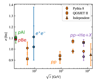
Figure 2: A compilation of values of the coalescence parameter $\sigma$, obtained from fits to various experimental data on antideuteron and antihelium-3 production in $pp$ [21, 22], $pN$ [23], and $e^{+}e^{-}$ [24, 25] collisions using Pythia 8 (circles) and QGSJET-II-04m (squares). The triangular data point is obtained from a femtroscopy experiment [20], and is thus independent on the event generator. The fitting is explained in Ref. [19] and references therein.

3 Secondary production of antinuclei

3.1 Comparison with parametrisation methods

Traditionally, the production of a nucleus with mass number $A$ has been parametrised by the proton spectrum as

$$E_{A}\derivative[3]{N_{A}}{P_{A}}=B_{A}\left(E_{N}\derivative[3]{N_{p}}{p_{p}}\right)^{A},$$ (3)

where $B_{A}$ is known as the coalescence factor. In the limit of isotropic nucleon yields, $B_{A}$ is a constant that scales with the nucleon emission volume as $B_{A}\propto V^{A-1}$ if the coalescence condition is evaluated in position space, and with the coalescence momentum as $B_{A}\propto p_{0}^{3A-3}$ if evaluated in momentum space. In small interacting systems, such as $pp$, $pN$ and $e^{+}e^{-}$ collisions or dark matter annihilations, this approximation is not valid since the nucleon yield is highly non-isotropic. Even so, the approximation (3) is often used in astrophysical studies due to its simplicity.

Another reason for deviations from the simple relation (3) is the missing phase-space suppression close to the production threshold. Since the production channels with the minimal number of particles, compatible with baryon number conservation, will dominate close to the threshold, one can approximate the suppression at low collision energies and high secondary nucleus energies as a pure phase-space suppression, assuming an isotropic matrix element (see e.g. Refs. [26, 27, 28]). Thus, the approximation (3) can be improved if we include a phase-space suppression factor

$$R_{N}(x)\equiv\frac{\Phi_{N}(x;m_{p})}{\Phi_{N}(x;0)},$$ (4)

where $x=\sqrt{s+Am_{p}^{2}-2\sqrt{s}\tilde{E}_{A}}$ describes the energy available in the center of mass (CoM) frame, and $\tilde{E}_{A}$ is the nucleus energy in the CoM frame. One can compute the phase-space integrals,

$$\Phi_{N}(x;m_{p})=\left[\prod_{i=1}^{N}\int\frac{\differential[3]{p_{i}}}{(2\pi)^{3}2E_{i}}\right](2\pi)^{4}\delta^{(3)}\left(\sum_{i=1}^{N}\boldsymbol{p}_{i}\right)\delta\left(\sum_{i=1}^{N}E_{i}-x\right),$$ (5)

with the integration volume being the full allowed phase-space, numerically using the method described in Ref. [29] (see Fig. 15 in Ref. [26] for a plot). This method has a major perk compared to a Monte Carlo treatment: It is significantly less computationally demanding. As in the case of the WiFunC model, the method contains no free parameters since the coalescence factor can be obtained from femtoscopy experiments [26, 30, 31]. However, the suppression factor is not exact and two-particle correlations are not taken into account, meaning that one may expect the method to give inaccurate results. For instance, at low energies near the threshold, the model is expected to overproduce nuclei since it does not take into account anti-correlations. Furthermore, the coalescence factor $B_{A}$ is typically determined in a kinematical regime not relevant for cosmic ray studies. As such, results obtained within this approximation have to be interpreted with care.

In order to verify the importance of using a Monte Carlo description, we plot in Fig. 3 the antideuteron (left) and antihelium-3 (right) spectra ${\rm d}N/{\rm d}E={\sigma_{\rm inel}}^{-1}{\rm d}\sigma_{\rm inel}/{\rm d}E$ obtained using Eqs. (3) and (4) (solid lines) and the WiFunC model (dashed lines) for various primary energies. The shaded areas correspond to the ranges $B_{2}=(0.75,2.4)\cdot 10^{-2}$ and $B_{3}=(2,20)\cdot 10^{-3}$ obtained from femtoscopy experiments [26]. Note that QGSJET-II-04m was used to obtain the antiproton spectrum, and that using instead a parametrisation of the antinucleon spectrum would lead to larger differences. While the phase-space suppression factor captures well the overall behaviour of the suppression for high secondary energies, there are large differences near the production threshold at low energies. These differences are much larger for helium-3 than for deuteron. A reason for these differences is that the parametrisation fails to account for the fact that certain processes are kinematically allowed but forbidden by conservation laws, e.g. for baryon number. In particular, antideuterons may be produced using parametrisations via the (forbidden) process $pp\to pp\bar{p}\bar{n}$. Furthermore, in high energy collisions and near the threshold, parametrisations fail to describe the momentum (anti-) correlations that may enhance or lower the antinuclei production [32]. Although the parametrisation (3) describes (within the experimental and theoretical uncertainties in $B_{A}$) the overall yield of antinuclei sufficiently well for order-of-magnitude estimates, an accurate Monte Carlo description is therefore needed if one aims to reduce the uncertainties in the theoretical predictions.

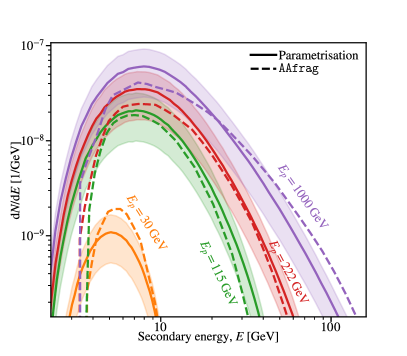
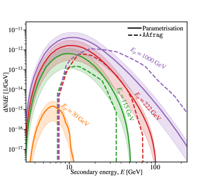
Figure 3: The antideuteron (left) and antihelium-3 (right) spectra obtained using Eqs. (3) and (4) (solid lines) and the WiFunC model (dashed lines). The results are shown for primary energies of 21 GeV (blue), 30 GeV (orange), 115 GeV (green), 222 GeV (red) and 1000 GeV (purple).

3.2 Nuclear enhancement

One of the major advantages of the WiFunC model and the use of a Monte Carlo generator is that one can describe the production of antideuteron and antihelium-3 in point-like and extended processes without any free parameters. In particular, one can avoid the use of a “nuclear enhancement factor”, which is otherwise required if the primary and/or the target is a nucleus. Previous studies like those of Refs. [33, 34] had to assume that the nuclear enhancement is constant and coincides with the one for antiproton production. In fact, these assumptions are invalid, as we shall demonstrate below.

To discuss the nuclear enhancement of secondary fluxes analytically, it is convenient to consider the case when the primary cosmic ray spectra can be approximated by power laws, $I_{A_{i}}(E_{0})\propto E_{0}^{-\alpha_{i}}$, with $\alpha_{i}$ being the slope and $E_{0}$ the energy per nucleon. In such a case, the contribution $q_{X}^{A_{i}p}$ to the secondary flux of particles $X$ ($e^{\pm}$, $\gamma$, $\nu$, or $\bar{p}$) from interactions of primary nuclei $A_{i}$ with protons from the interstellar medium is proportional to the weighted moment of the corresponding production spectrum (see, e.g. [7]):

$$q_{X}^{A_{i}p}(E)\propto Z_{X}^{A_{i}p}(E,\alpha_{i})\,,$$ (6)

with

$$Z_{X}^{A_{i}p}(E,\alpha_{i})=\int_{0}^{1}\!\mathrm{d}z\;z^{\alpha_{i}-1}\;\frac{\mathrm{d}\sigma_{A_{i}p\rightarrow X}(E/z,z)}{\mathrm{d}z}\,.$$ (7)

Then the nuclear enhancement can be quantified by the ratio $Z_{X}^{A_{i}p}(E,\alpha_{i})/Z_{X}^{pp}(E,\alpha_{i})$ which would coincide with the ratio of the respective contributions to the secondary flux of interest, $q_{X}^{A_{i}p}/q_{X}^{pp}$, if the primary proton and nuclei flux would be the same. In the limit of very high energies, one obtains an $A$ enhancement for that ratio [7, 12],

$$\varepsilon_{X}^{A_{i}p}(E)\equiv Z_{X}^{A_{i}p}(E,\alpha_{i})/Z_{X}^{pp}(E,\alpha_{i})\rightarrow A_{i}\,.$$ (8)

This simple result follows from two important features of nucleus-proton (or, more generally, nucleus-nucleus) interactions. First, the forward (i.e. large $z$) spectrum for any secondary particle $X$ in collisions of a nucleus $A$ with protons can be approximated by the one for a superposition of $\langle n_{A}^{\rm w}\rangle$ independent $pp$ collisions,

$$\left.\frac{dn_{A_{i}p\rightarrow X}(E_{0},z)}{dz}\right|_{z\rightarrow 1}\simeq\langle n_{A}^{\rm w}(E_{0})\rangle\,\frac{dn_{pp\rightarrow X}(E_{0},z)}{dz}\,.$$ (9)

Here, the average number $\langle n_{A}^{\rm w}\rangle$ of interacting (“wounded”) projectile nucleons satisfies [35]

$$\langle n_{A}^{\rm w}(E_{0})\rangle\simeq\frac{A\,\sigma^{\rm inel}_{pp}(E_{0})}{\sigma^{\rm inel}_{Ap}(E_{0})}\,,$$ (10)

with $\sigma^{\rm inel}_{pp}$ and $\sigma^{\rm inel}_{Ap}$ as the inelastic cross sections of $pp$ and $Ap$ collisions, respectively. Inserting Eq. (10) into (9) and substituting the result in (7), one arrives at Eq. (8).

Let us consider now the production of light nuclei. For definiteness, we will discuss the case of antideuterons. The crucial difference to the picture described above is that this process proceeds via the coalescence mechanism and thus involves the double differential spectra of produced antiprotons and antineutrons, $\mathrm{d}^{2}\sigma_{Ap\rightarrow\bar{p}+\bar{n}}/{\mathrm{d}z_{\bar{p}}\mathrm{d}z_{\bar{n}}}$. In nucleus-proton collisions, the coalescing antiproton and antineutron are typically created in rescatterings of different projectile nucleons off the target proton [8]. Consequently, the forward-production spectra of antideutrons become proportional to the number of possible pair-wise nucleon-proton rescattering processes, $\propto n_{A}^{\rm w}(n_{A}^{\rm w}-1)$. Thus, at sufficiently high energies and for large $A$, the nuclear enhancement for $\bar{d}$ production should satisfy

$$\varepsilon_{\bar{d}}^{Ap}(E)\propto\frac{A^{2}\sigma^{\rm inel}_{pp}(E)}{\sigma^{\rm inel}_{Ap}(E)}\simeq A^{4/3},$$ (11)

with $E$ as the energy per nucleon for $\bar{d}$. In the last step, we assumed for illustration a simple $A^{2/3}$ scaling for the $Ap$ cross sections.

In Fig. 4, we plot the calculated energy dependence of the enhancement factors $\varepsilon_{\bar{d}}^{AB}(E)=q_{X}^{AB}/q_{X}^{pp}$, for $AB={\rm He}p$, $p{\rm He}$, and ${\rm He}{\rm He}$ and assuming the same primary proton and helium flux. At the highest energies, $\varepsilon_{\bar{d}}^{{\rm He}p}$ is larger than four and increasing towards the asymptotic limit, Eq. (11). In contrast, the behaviour of $\varepsilon_{\bar{d}}^{AB}(E)$ changes drastically in the low-energy limit. Such a trend has been previously observed and explained in Ref. [12], for the case of $\bar{p}$ production: Because of the relatively high proton mass, at low energies the integral in Eq. (7) is no longer dominated by forward (large $z$) $\bar{p}$ production. Instead, important contributions come from the central (in the center of mass frame) and backward production, such that the reasoning which lead to Eq. (8) becomes inapplicable. The same considerations fully apply to the case of antideutron production. Moreover, regarding antideutron production in proton-helium collisions, the coalescing $\bar{p}$ and $\bar{n}$ are predominantly produced in inelastic rescatterings on different target nucleons. As a result, the energy threshold for $\bar{d}$ production is lower than in $pp$ interactions, and gives rise to a large nuclear enhancement close to the production threshold.

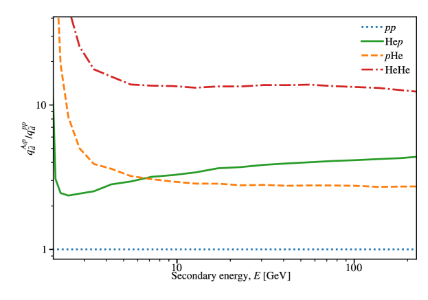
Figure 4: The nuclear enhancement factors $\varepsilon_{\bar{d}}^{AB}(E)=q_{X}^{A_{A}B}/q_{X}^{pp}$ as function of the total energy for $AB={\rm He}p$, $p{\rm He}$, and ${\rm He}{\rm He}$ collisions.

3.3 The use of event generators and the interpretation of accelerator data

Currently, the best experimental data on antinuclei production, e.g. from the ALICE experiment, are obtained at energies and in kinematical regions that are not relevant for astrophysical studies. Fitting phenomenological coalescence models to such data leads to a biased model with a reduced predictive power. Therefore it is important to always assess the applicability of an event generator, e.g., by comparing with antiproton data obtained under the same conditions, when comparing the coalescence model to experimental data. For example, QGSJET does not reproduce well the slope of the antiproton spectrum at 2.76 and 7 TeV measured by ALICE [8]. Therefore, a re-weighting of the antiproton spectrum at these energies has been performed in order to obtain a more precise prediction for the coalescence factor [8] in Fig. 1. If QGSJET-II-04m is blindly applied to the 7 TeV ALICE data, the obtained value for the coalescence parameter $\sigma$ is 1.4 fm, while adjusting the results to the antiproton data yields 1.1 fm [8, 19].

4 Program structure and example output

For convenience of both the young generation and ancient users, the program AAfrag 2 exists as both Python 3 and Fortran 90 versions.

4.1 Purpose and method

Aafrag 2 is a tool that interpolates results relevant for secondary interactions in cosmic ray studies from the Monte Carlo simulation QGSJET-II-04m. The calculation of the production cross section of photons, neutrinos, electrons, positrons, (anti-) protons and (anti-) neutrons in $pp$, $p$He, He$p$, HeHe, C$p$, Al$p$, Fe$p$ interactions, as well as production cross section of antideuteron and antihelium-3 in $pp$, $p$He, He$p$, HeHe, $\bar{p}p$ and $\bar{p}$He interactions, are included. The tool allows the users to benefit from the advantages of a Monte Carlo simulation, with minimal computational effort. The calculations of photons, neutrinos, electrons, positrons, (anti-) protons and (anti-) neutrons were discussed in Ref. [9], while the cases of antideuteron and antihelium were treated in this work.

The results from the Monte Carlo simulations were stored in tables, and the main purpose of AAfrag 2 is to provide the user with convenient interpolation routines. The interpolation is performed using bilinear interpolation, with a fill value 0 outside the data range.

The Fortran 90 program includes its own interpolation routines and is thus self-consistent, while the Python 3 program depends on the numpy, scipy and matplotlib libraries.

4.2 Program structure

The Fortran 90 program consists of two Fortran files, AAfrag2.f90 and user.f90, in addition to the numerical tables in the Tables folder. The file AAfrag2.f90 contains the module spectra which is used to store physical parameters and the loaded tables, the main program, subroutines used to initialise and load the tables, and the interpolation functions. Meanwhile, the file user.f90 contains an example calculation. For the normal user, only changes in user.f90 are necessary. The main program calls init which loads all the tables and stores the data in the variables defined in the module spectra. Next, the subroutine user_main in user.f90 is called. Users must adapt this subroutine to their specific needs.

The Python 3 program is contained in AAfrag2.py, in addition to the numerical tables in the Tables folder. The Python functions have the same names and input parameters as the Fortran subroutines and functions. The script contains an example calculation that is executed when the script is run as a standalone. The user can either change the example portion of the script, or import the file as a module.

4.3 Functions

The program includes five functions that are intended to be used by the user (spec_gam, spec_nu, spec_elpos, spec_pap, spec_nan, spec_ad, spec_ah) which interpolate the production spectra of secondaries $\{\gamma,$ $\nu_{i},$ $e^{-},$ $e^{+},$ $p,$ $\bar{p},$ $n,$ $\bar{n},$ $\bar{d}$, ${}^{3}\bar{\rm He}$+${}^{3}\bar{\rm H}\}$ in various cosmic ray interactions. The functions have the same input parameters: (E_p, E_s, q, k). Here, E_p is the total energy of the primary nucleus in GeV, E_s is the kinetic energy of the produced secondary in GeV, q denotes the particle species as detailed in Tab. 1, and k denotes the interaction type as detailed in Tab. 2. The output is the production spectrum $E_{s}^{2}\derivative*{\sigma^{k}(E_{p},E_{s})}{E_{s}}$ in GeV mb. An example of their uses is given in the example programs.

Function	$q=1$	$q=2$	$q=3$	$q=4$
spec_nu	$\nu_{e}$	$\bar{\nu}_{e}$	$\nu_{\mu}$	$\bar{\nu}_{\mu}$
spec_elpos	$e^{-}$	$e^{+}$	–	–
spec_pap	$p$	$\bar{p}$	–	–
spec_nan	$n$	$\bar{n}$	–	–
spec_gam	$\gamma$	–	–	–
spec_ad	$\bar{d}$	–	–	–
spec_ah	${}^{3}\bar{\rm He}+{{}^{3}}\bar{\rm H}$	–	–	–

Table 1: The particle type determined by the parameter $q$.

	$k=1$	$k=2$	$k=3$	$k=4$	$k=5$	$k=6$	$k=7$	$k=8$	$k=9$
Beam–Target	$p$–$p$	$p$–He	He–$p$	He–He	C–$p$	Al–$p$	Fe–$p$	$\bar{p}$–$p$	$\bar{p}$–He
Mass number	1–1	1–4	4–1	4–4	12–1	26–1	56–1	1–1	1–4

Table 2: Reaction type determined by the parameter $k$. Reactions 5–7 are not implemented for antideuteron (spec_ad) and antihelium-3 (spec_ah), while reactions 8–9 are exclusively implemented for them.

4.4 Example output

The output of the example calculation are the files spec_gam, spec_nu, spec_elpos, spec_aprot, spec_aneut, spec_adeut and spec_ahel. They contain respectively the production spectra of photons, neutrinos, electrons and positrons, antiprotons, antineutrons, antideuterons, and antihelium-3. The result is plotted in Fig. 5 for $pp$ collisions at 100 GeV.

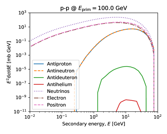
Figure 5: Production spectrum of antiprotons, antineutrons, antideuterons, neutrinos, positrons and electrons in $pp$ collisions with primary energy of 100 GeV. The figure is obtained by running the example programs included in AAfrag2.

5 Summary

Astrophysical antideuteron and antihelium-3 are ideal probes for new, exotic physics due to the suppressed background at low energies. Therefore, we made our predictions for the production cross sections of antideuteron and antihelium-3 in $pp$, $p$He, He$p$, HeHe, $\bar{p}p$ and $\bar{p}$He collisions at energies relevant for secondary production in the Galaxy publicly available through the interpolation subroutines AAfrag. The predictions are based on QGSJET-II-04m and the state of the art coalescence model evaluated on an event-by-event basis. Furthermore, we commented on the use of Monte Carlo generators to predict antinuclei fluxes, the use of a nuclear enhancement factor to predict secondary cosmic ray fluxes, and the effect of two-particle momentum correlations provided by a Monte Carlo.

6 Acknowledgements

This research was supported by the Munich Institute for Astro- and Particle Physics (MIAPP) which is funded by the Deutsche Forschungsgemeinschaft (DFG, German Research Foundation) under Germany’s Excellence Strategy – EXC-2094 – 390783311. S.O. acknowledges support from the Deutsche Forschungsgemeinschaft (project number 465275045).

References

- [1] A. Neronov, D. V. Semikoz, A. M. Taylor, Low-energy break in the spectrum of Galactic cosmic rays, Phys. Rev. Lett. 108 (2012) 051105. arXiv:1112.5541, doi:10.1103/PhysRevLett.108.051105.
- [2] M. Ackermann, et al., Fermi-LAT Observations of the Diffuse Gamma-Ray Emission: Implications for Cosmic Rays and the Interstellar Medium, Astrophys. J. 750 (2012) 3. arXiv:1202.4039, doi:10.1088/0004-637X/750/1/3.
- [3] M. Kachelrieß, S. Ostapchenko, Deriving the cosmic ray spectrum from gamma-ray observations, Phys. Rev. D 86 (2012) 043004. arXiv:1206.4705, doi:10.1103/PhysRevD.86.043004.
- [4] F. Donato, N. Fornengo, P. Salati, Anti-deuterons as a signature of supersymmetric dark matter, Phys. Rev. D62 (2000) 043003. arXiv:hep-ph/9904481, doi:10.1103/PhysRevD.62.043003.
- [5] P. von Doetinchem, et al., Cosmic-ray Antinuclei as Messengers of New Physics: Status and Outlook for the New Decade, JCAP 08 (2020) 035. arXiv:2002.04163, doi:10.1088/1475-7516/2020/08/035.
- [6] M. Kachelrieß, S. Ostapchenko, Neutrino yield from Galactic cosmic rays, Phys. Rev. D 90 (8) (2014) 083002. arXiv:1405.3797, doi:10.1103/PhysRevD.90.083002.
- [7] M. Kachelrieß, I. V. Moskalenko, S. S. Ostapchenko, Nuclear enhancement of the photon yield in cosmic ray interactions, Astrophys. J. 789 (2014) 136. arXiv:1406.0035, doi:10.1088/0004-637X/789/2/136.
- [8] M. Kachelrieß, S. Ostapchenko, J. Tjemsland, Revisiting cosmic ray antinuclei fluxes with a new coalescence model, JCAP 08 (2020) 048. arXiv:2002.10481, doi:10.1088/1475-7516/2020/08/048.
- [9] M. Kachelrieß, I. V. Moskalenko, S. Ostapchenko, AAfrag: Interpolation routines for Monte Carlo results on secondary production in proton-proton, proton-nucleus and nucleus-nucleus interactions, Comput. Phys. Commun. 245 (2019) 106846. arXiv:1904.05129, doi:10.1016/j.cpc.2019.08.001.
- [10] S. Ostapchenko, Monte Carlo treatment of hadronic interactions in enhanced Pomeron scheme: I. QGSJET-II model, Phys. Rev. D83 (2011) 014018. arXiv:1010.1869, doi:10.1103/PhysRevD.83.014018.
- [11] S. Ostapchenko, QGSJET-II: physics, recent improvements, and results for air showers, EPJ Web Conf. 52 (2013) 02001. doi:10.1051/epjconf/20125202001.
- [12] M. Kachelrieß, I. V. Moskalenko, S. S. Ostapchenko, New calculation of antiproton production by cosmic ray protons and nuclei, Astrophys. J. 803 (2) (2015) 54. arXiv:1502.04158, doi:10.1088/0004-637X/803/2/54.
- [13] S. Koldobskiy, M. Kachelrieß, A. Lskavyan, A. Neronov, S. Ostapchenko, D. V. Semikoz, Energy spectra of secondaries in proton-proton interactions, Phys. Rev. D 104 (12) (2021) 123027. arXiv:2110.00496, doi:10.1103/PhysRevD.104.123027.
- [14] A. Schwarzschild, C. Zupancic, Production of Tritons, Deuterons, Nucleons, and Mesons by 30-GeV Protons on A-1, Be, and Fe Targets, Phys. Rev. 129 (1963) 854–862. doi:10.1103/PhysRev.129.854.
- [15] S. T. Butler, C. A. Pearson, Deuterons from high-energy proton bombardment of matter, Phys. Rev. 129 (2) (1963) 836–842. doi:10.1103/PhysRev.129.836.
- [16] M. Kachelrieß, S. Ostapchenko, J. Tjemsland, Alternative coalescence model for deuteron, tritium, helium-3 and their antinuclei, Eur. Phys. J. A56 (1) (2020) 4. arXiv:1905.01192, doi:10.1140/epja/s10050-019-00007-9.
- [17] M. Kachelrieß, S. Ostapchenko, J. Tjemsland, On nuclear coalescence in small interacting systems, Eur. Phys. J. A 57 (5) (2021) 167. arXiv:2012.04352, doi:10.1140/epja/s10050-021-00469-w.
- [18] V. I. Zhaba, Deuteron: analytical forms of wave function and density distribution, APS Physics 42 (2017) 191–195. arXiv:1802.02778, doi:10.24144/2415-8038.2017.42.191-195.
- [19] J. Tjemsland, Formation of light (anti)nuclei, PoS TOOLS2020 (2021) 006. arXiv:2012.12252, doi:10.22323/1.392.0006.
- [20] S. Acharya, et al., Search for a common baryon source in high-multiplicity pp collisions at the LHC, Phys. Lett. B 811 (2020) 135849. arXiv:2004.08018, doi:10.1016/j.physletb.2020.135849.
- [21] S. Acharya, et al., Production of deuterons, tritons, 3He nuclei and their antinuclei in pp collisions at = 0.9, 2.76 and 7 TeV, Phys. Rev. C 97 (2) (2018) 024615. arXiv:1709.08522, doi:10.1103/PhysRevC.97.024615.
- [22] S. Henning, et al., Production of Deuterons and anti-Deuterons in Proton Proton Collisions at the CERN ISR, Lett. Nuovo Cim. 21 (1978) 189. doi:10.1007/BF02822248.
- [23] W. Bozzoli, A. Bussiere, G. Giacomelli, E. Lesquoy, R. Meunier, L. Moscoso, A. Muller, D. E. Plane, F. Rimondi, S. Zylberajch, Search for Longlived Particles in 200-GeV/ Proton - Nucleon Collisions, Nucl. Phys. B 159 (1979) 363–382. doi:10.1016/0550-3213(79)90340-7.
- [24] S. Schael, et al., Deuteron and anti-deuteron production in e+ e- collisions at the Z resonance, Phys. Lett. B 639 (2006) 192–201. arXiv:hep-ex/0604023, doi:10.1016/j.physletb.2006.06.043.
- [25] R. Akers, et al., Search for heavy charged particles and for particles with anomalous charge in collisions at LEP, Z. Phys. C 67 (1995) 203–212. doi:10.1007/BF01571281.
- [26] K. Blum, K. C. Y. Ng, R. Sato, M. Takimoto, Cosmic rays, antihelium, and an old navy spotlight, Phys. Rev. D96 (10) (2017) 103021. arXiv:1704.05431, doi:10.1103/PhysRevD.96.103021.
- [27] R. P. Duperray, K. V. Protasov, A. Y. Voronin, Anti-deuteron production in proton proton and proton nucleus collisions, Eur. Phys. J. A 16 (2003) 27–34. arXiv:nucl-th/0209078, doi:10.1140/epja/i2002-10074-0.
- [28] R. P. Duperray, K. V. Protasov, L. Derome, M. Buenerd, A Model for A = 3 anti-nuclei production in proton nucleus collisions, Eur. Phys. J. A 18 (2003) 597–604. arXiv:nucl-th/0301103, doi:10.1140/epja/i2003-10099-9.
- [29] F. E. James, Monte Carlo phase space, CERN, Geneva, 1968, p. 41 p, [numerical implementation given in the GENBOD subroutine (W515) in the CERNLIB Fortran libraries]. doi:10.5170/CERN-1968-015.
- [30] K. Blum, M. Takimoto, Nuclear coalescence from correlation functions, Phys. Rev. C 99 (4) (2019) 044913. arXiv:1901.07088, doi:10.1103/PhysRevC.99.044913.
- [31] F. Bellini, K. Blum, A. P. Kalweit, M. Puccio, Examination of coalescence as the origin of nuclei in hadronic collisions, Phys. Rev. C 103 (1) (2021) 014907. arXiv:2007.01750, doi:10.1103/PhysRevC.103.014907.
- [32] L. A. Dal, M. Kachelrieß, Antideuterons from dark matter annihilations and hadronization model dependence, Phys. Rev. D86 (2012) 103536. arXiv:1207.4560, doi:10.1103/PhysRevD.86.103536.
- [33] S.-J. Lin, X.-J. Bi, P.-F. Yin, Expectations of the Cosmic Antideuteron Flux (2018). arXiv:1801.00997.
- [34] A. Ibarra, S. Wild, Determination of the Cosmic Antideuteron Flux in a Monte Carlo approach, Phys. Rev. D 88 (2013) 023014. arXiv:1301.3820, doi:10.1103/PhysRevD.88.023014.
- [35] A. Białas, M. Bleszynski, W. Czyz, , Nucl. Phys. B 111 (1976) 461.