Multi-scale Wasserstein Shortest-path Graph Kernels for Graph Classification

Abstract

Graph kernels are conventional methods for computing graph similarities. However, most of the R-convolution graph kernels face two challenges: 1) They cannot compare graphs at multiple different scales, and 2) they do not consider the distributions of substructures when computing the kernel matrix. These two challenges limit their performances. To mitigate the two challenges, we propose a novel graph kernel called the Multi-scale Wasserstein Shortest-Path graph kernel (MWSP), at the heart of which is the multi-scale shortest-path node feature map, of which each element denotes the number of occurrences of a shortest path around a node. A shortest path is represented by the concatenation of all the labels of nodes in it. Since the shortest-path node feature map can only compare graphs at local scales, we incorporate into it the multiple different scales of the graph structure, which are captured by the truncated BFS trees of different depths rooted at each node in a graph. We use the Wasserstein distance to compute the similarity between the multi-scale shortest-path node feature maps of two graphs, considering the distributions of shortest paths. We empirically validate MWSP on various benchmark graph datasets and demonstrate that it achieves state-of-the-art performance on most datasets.

I Introduction

Graph-structured data is ubiquitous in many scenarios, such as protein-protein interaction networks, social networks, citation networks, and cyber-physical systems. One interesting and fundamental problem with graph-structured data is quantifying their similarities, which can be measured by graph kernels. Most of the graph kernels belong to the family of the R-convolution kernels [1] that decompose graphs into substructures and compare them. There are many kinds of substructures used in graph kernels, such as walks [2, 3, 4], paths [5], subgraphs [6, 7, 8, 9], and subtree patterns [10, 11, 12, 13, 14, 15].

The R-convolution graph kernels have two main challenges. Firstly, when computing the similarity between two graphs, they count the number of occurrences of each unique substructure in each graph and aggregate the occurrences. Simple aggregation operation such as sum aggregation neglects the distributions of substructures in each graph, which might restrict their ability to capture complex relationships between substructures. Secondly, many R-convolution graph kernels cannot compare graphs at multiple different scales. For example, WL [12, 13] computes graph similarity at coarse scales, because subtrees only consider the whole neighborhood structures of nodes rather than single edges between two nodes; SP [5] computes the graph similarity at fine scales because shortest paths do not take neighborhood structures into account. In many real-world scenarios, graphs such as social networks have structures at multiple different scales, such as chains, rings, and stars. Graph kernels should not only differentiate the overall shape of graphs but also their small substructures.

To solve the first challenge, PM [16] eigendecomposes the adjacency matrix of a graph and embeds each node in the space spanned by the eigenvectors. The similarity between two graphs is computed by the Earth Mover’s Distance [17] or the Pyramid Match kernel [18, 19], considering the distributions of node embeddings. However, eigenvectors can only capture the global connectivity of a graph. Thus, PM cannot compare graphs at multiple different scales. WWL [15] adopts the Weisfeiler-Lehman test of graph isomorphism [20] to relabel each node. The new label of a node corresponds to the subtree pattern around it. WWL considers node labels as categorical embeddings. The similarity between two graphs is computed by the Wasserstein distance, using the normalized Hamming distance as the ground distance for categorical node embeddings. The distributions of subtree patterns are considered in the computation of graph similarity. But WWL cannot compare graphs at fine scales because of the utilization of the subtree patterns as used in WL.

To solve the second challenge, MLG [9] computes graph similarity at multiple different scales by applying recursively the Feature space Laplacian Graph (FLG) kernel on a hierarchy of nested subgraphs. Specifically, FLG is a variant of the Bhattacharyya kernel [21] that computes the similarity between two graphs by using their Laplacian matrices. The sizes of subgraphs increase with the increasing level of the hierarchy, including the different scales of the graph structure around a node. However, MLG does not take the distributions of node embeddings (denoted by the rows of the graph Laplacian matrix) into account when computing graph similarity.

Considering that many real-world graphs have the small world property [22], i.e., the mean shortest-path length is small, the shortest-path graph kernel (SP) [5] fits these kind of graphs well. We study SP in this paper. The substructure used in SP is the shortest path which is represented by a triplet whose elements are the labels of source and sink nodes of this shortest path and its length. The triplet representation is coarse and may lose information because it neglects the labels of the intermediate nodes in a shortest path. In this paper, each shortest path is denoted by the concatenation of the labels of all the nodes in this shortest path rather than the simple triplet representation. Guided by the small world property, we build a truncated BFS (Breadth-First Search) tree of depth $d$ rooted at each node in a graph and only consider the shortest paths starting from the root to any other node in the truncated BFS tree. In this way, the maximal length of a shortest path in a graph is limited to $d$. To mitigate the two challenges, we propose a multi-scale shortest-path graph/node feature map, capturing the multiple different scales of the graph structure. The shortest-path graph/node feature map is constructed by counting the number of occurrences of shortest paths in a graph or around a node. As aforementioned, SP cannot compare graphs at multiple different scales. To integrate the multiple different scales of the graph structure into the shortest-path graph/node feature map, we allow components in a shortest path to be BFS trees of different depths. To represent such kind of shortest paths, we project each BFS tree into an integer label by an injective hash method, i.e., hashing the same BFS trees to the same integer label and different BFS trees to different integer labels. Thus, the representation of such kind of shortest paths is just the concatenation of the integer labels of all BFS trees in this shortest path. We concatenate the multiple different scales of shortest-path graph/node feature maps and adopt the Wasserstein distance to compute graph similarity, capturing the distributions of shortest paths.

Our main contributions can be summarized as follows:

• We build a truncated BFS tree of limited depth rooted at each node to restrict the maximal length of shortest paths in a graph, guided by the small world property. Each shortest path is represented by the concatenation of all its node labels rather than the simple triplet representation, considering all node labels in this shortest path.

• We propose the multi-scale shortest-path graph/node feature map that incorporates the different scales of the graph structure into the shortest-path graph/node feature map and can compare graphs at multiple different scales. The different scales of the graph structure are captured by the truncated BFS trees of varying depths rooted at each node.

• We develop a graph kernel called MWSP (for Multi-scale Wasserstein Shortest-Path graph kernel) that employs the Wasserstein distance to compute the similarity between the multi-scale shortest-path node feature maps of two graphs, capturing the distributions of shortest paths.

• We show in the experiments that our graph kernel MWSP achieves the best classification accuracy on most benchmark datasets.

II Related Work

Random walk graph kernels [2, 3] decompose graphs into their substructures random walks and compute the number of matching random walks from two graphs, which can be transformed to perform random walks on the direct product graph of two input graphs. Gärtner et al. [2] introduce the concept of direct product graph and derive two closed-form random walk graph kernels, which are called the geometric kernel and the exponential kernel, respectively. The former kernel is based on the personalized PageRank diffusion [23] while the latter kernel is based on the heat kernel diffusion [24]. RetGK [4] proposes a random walk graph kernel that is applicable on both attributed and non-attributed graphs. Each graph is represented by a multi-dimensional tensor that is composed of the return probability vectors of random walks starting and ending with the same nodes and other discrete or continuous attributes of nodes. The multi-dimensional tensor is embedded into the Hilbert space by maximum mean discrepancy (MMD) [25] and the random walk graph kernels are computed. Borgwardt et al. [5] propose the shortest-path graph kernel (SP) that decomposes graphs into shortest paths between each pair of nodes in graphs. SP counts the number of pairs of matching shortest paths that have the same source and sink node labels and the same length in two graphs.

The graphlet kernel (GK) [6] decomposes graphs into substructures called graphlets [26]. The number of nodes a graphlet can have is restricted to five for the efficiency of enumeration. Even by this restriction, exhaustive enumeration of all graphlets in a graph is still prohibitively expensive. Thus, Shervashidze et al. [6] propose to speed up the enumeration by using the method of random sampling. Costa et al. [7] develop a graph kernel called the Neighborhood Subgraph Pairwise Distance Kernel (NSPDK) that decomposes a graph into all pairs of neighborhood subgraphs of small radium at increasing distances. To speed up the Gram matrix computation, they use a fast graph invariant string encoding for the pairs of neighborhood subgraphs. Kondor et al. [9] propose a multiscale Laplacian graph kernel for capturing the graph structure at multiple different scales. To solve the graph invariance problem, the feature space Laplacian graph kernel (FLG) is developed. Then, each node is associated with a subgraph centered around it, and the FLG kernel between each pair of these subgraphs is computed. To compute graph similarity at multiple different scales, the size of subgraphs is increased and the FLG kernel is recursively applied on these larger subgraphs.

Weisfeiler-Lehman subtree kernel (WL) [12, 13] augments each node using the first-order Weisfeiler-Lehman test of graph isomorphism [20]. It concatenates the labels of a node and all its neighboring nodes into a string and hashes the concatenated labels into new labels, aggregating neighborhood information around a node. WWL [15] extends WL to graphs with continuous attributes by considering each graph as a set of node embeddings and using the Wasserstein distance to compute the similarity between the two sets of node embeddings. Each node is associated with two kinds of features, one of which is the subtree feature map generated by WL and the other of which is continuous attributes. The continuous attributes of each node are propagated to its neighboring nodes by an average aggregation operator, which is similar to the layer-wise propagation rule of Graph Convolutional Networks (GCN) [27]. Our method MWSP also uses the Wasserstein distance to compute the similarity between the shortest-path node feature maps of two graphs. OA [28] develops base kernels that generate graph hierarchies, from which the optimal assignment kernels are computed and guaranteed positive semidefinite. The optimal assignment kernels provide a more valid notion of graph similarity, which is integrated into the WL to improve its performance. FWL [29] is based on a filtration kernel that compares Weisfeiler-Lehman subtree feature occurrence distributions (filtration histograms) over sequences of nested subgraphs, which are generated by sequentially considering all the edges whose weights are less than a changing threshold. This strategy not only provides graph features on different levels of granularities but also considers the life span of graph features. FWL’s expressiveness is more powerful than the ordinary WL.

DGK utilizes word2vec [30] to learn latent representations for substructures, such as graphlets, shortest paths, and subtree patterns. The similarity matrix between substructures is computed and integrated into the computation of the graph kernel matrix. Nikolentzos et al. [16] use the eigenvectors of the graph adjacency matrices as graph embeddings and propose two graph kernels to compute the similarity between two graph embeddings. The first graph kernel uses the Earth Mover’s Distance [17] to compute the distance between two graph embeddings; and the second one uses the Pyramid Match kernel [18, 19] to find an approximate correspondence between two graph embeddings. HTAK [31] transitively aligns the vertices between graphs through a family of hierarchical prototype graphs, which are generated by the k-means clustering method. Graph Neural Tangent Kernel (GNTK) [32] is inspired by the connections between over-parameterized neural networks and kernel methods [33, 34]. It inherits both the advantages of GNN and graph kernels, i.e., extracting powerful features from graphs as GNN and being easy to train and analyze as graph kernels. It is equivalent to an infinitely wide GNN trained by gradient descent. GNTK is proven to learn a class of smooth functions on graphs. GraphQNTK [35] is an extension of GNTK by introducing the attention mechanism and quantum computing into GNTK’s structure and computation.

III Multi-scale Wasserstein Shortest-path Graph Kernels

III-A Shortest-Path Graph Feature Map

The shortest-path graph kernel (SP) [5] uses a triplet that contains the labels of the source and sink nodes and the length of a shortest path as its representation. This coarse representation loses the information of the intermediate nodes. To alleviate this situation, we consider all the information of nodes in a shortest path. We first describe the representation of a shortest path used in our graph kernel as follows:

Definition 1 (Shortest-path Representation).

Given an undirected labeled graph $\mathcal{G}=(\mathcal{V},\mathcal{E},l)$, we build a truncated BFS tree $\mathcal{T}=(\mathcal{V}^{\prime},\mathcal{E}^{\prime},l)$ ($\mathcal{V}^{\prime}\subseteq\mathcal{V}$ and $\mathcal{E}^{\prime}\subseteq\mathcal{E}$) of depth $d$ rooted at each node $v\in\mathcal{V}$. $v$ is called root. For each node $v^{\prime}\in\mathcal{V}^{\prime}$, a shortest path is constructed by concatenating all the distinct nodes and edges from the root $v$ to $v^{\prime}$, i.e., $P=``v,v_{1},v_{2},\ldots,v^{\prime}"$. The shortest-path representation is the concatenated labels of all the nodes in this shortest path, i.e., $l(P)=``l(v),l(v_{1}),l(v_{2}),\ldots,l(v^{\prime})"$.

Guided by the small world property, we build a truncated BFS tree of depth $d$ rooted at each node to restrict the maximal length of the shortest path in a graph. Figure 1(a) and (b) show two undirected labeled graphs $\mathcal{G}_{1}$ and $\mathcal{G}_{2}$, respectively. Figure 1(c) and (d) show two truncated BFS trees of depth $d=1$ rooted at the nodes with label 4 in $\mathcal{G}_{1}$ and $\mathcal{G}_{2}$, respectively. All the shortest paths starting from the root of the BFS tree in Figure 1(c) can be represented by $``4",``4,1",``4,3",``4,3"$ and those of the root of the BFS tree in Figure 1(d) can be represented by $``4",``4,1",``4,2",``4,3",``4,3"$. Note that we also consider a shortest path of length zero, which only contains one node that plays the role of both source and sink node. And we only consider the shortest paths in BFS trees instead of finding all the shortest paths in a graph as used in SP, considering the small world property. For a set of graphs, we construct a truncated BFS tree of depth $d$ rooted at each node and generate all its shortest paths, which are kept in a multiset $\mathcal{M}$.

(a) An undirected labeled graph $\mathcal{G}_{1}$.

(b) An undirected labeled graph $\mathcal{G}_{2}$.

(c) A truncated BFS tree of depth one rooted at the node with label 4 in graph $\mathcal{G}_{1}$.

(d) A truncated BFS tree of depth one rooted at the node with label 4 in graph $\mathcal{G}_{2}$.

Figure 1: Illustration of the shortest paths in graphs. $\Sigma=\{1,2,3,4\}$.

We define the shortest-path graph feature map as follows:

Definition 2 (Shortest-path Graph Feature Map).

Let $\mathcal{M}_{1},\mathcal{M}_{2},\ldots,\mathcal{M}_{n}$ be the multisets of shortest paths extracted from graphs $\mathcal{G}_{1},\mathcal{G}_{2},\ldots,\mathcal{G}_{n}$, respectively. Let the union of all the multisets be a set $\mathcal{U}=\mathcal{M}_{1}\cup\mathcal{M}_{2}\cup\cdots\cup\mathcal{M}_{n}=\{l(P_{1}),l(P_{2}),\cdots,l(P_{|\mathcal{U}|})\}$. Define a map $\psi:\{\mathcal{G}_{1},\mathcal{G}_{2},\ldots,\mathcal{G}_{n}\}\times\Sigma\rightarrow\mathbb{N}$ such that $\psi(\mathcal{G}_{i},l(P_{j}))$ ($1\leq i\leq n,1\leq j\leq|\mathcal{U}|$) is the number of occurrences of the shortest path $l(P_{j})$ in graph $\mathcal{G}_{i}$. Then, the shortest-path graph feature map of $\mathcal{G}_{i}$ is defined as follows:

$$\phi(\mathcal{G}_{i})=\left[\psi(\mathcal{G}_{i},l(P_{1})),\psi(\mathcal{G}_{i},l(P_{2})),\ldots,\psi(\mathcal{G}_{i},l(P_{|\mathcal{U}|}))\right]$$ (1)

III-B Multi-scale Shortest-path Graph Feature Map

In the last section, we decompose a graph into its substructures, i.e., shortest paths. However, shortest paths cannot reveal the structural or topological information of nodes. Thus, the shortest-path graph feature map can only capture graph similarity at fine scales. To capture graph similarity at multiple different scales, we focus on the different scales of the graph structure around a node.

To incorporate the multiple different scales of the graph structure into the shortest-path graph feature map, we first use the multiple different scales of the graph structure around a node to augment this node and then generate all the shortest paths starting from this node. Specifically, for each node in a shortest path $P=``v,v_{1},v_{2},\ldots,v^{\prime}"$, we build a truncated BFS tree of depth $k$ rooted at it, which captures the graph structure at the $k$-th scale around this node. And we have a shortest path $P$ that goes through a sequence of BFS trees $P=``\mathcal{T}_{v},\mathcal{T}_{v_{1}},\mathcal{T}_{v_{2}},\ldots,\mathcal{T}_{v^{\prime}}"$. Note that compared with the normal shortest path whose components are nodes, the shortest path in this work can contain BFS trees as its components.

Our next step is to represent such kinds of shortest paths. The difficulty is how to label each truncated BFS tree in a shortest path. Thus, we need to redefine the definition of the label function $l$ as follows: $l:\mathcal{T}\rightarrow\Sigma$ is a function that assigns labels from a set of positive integers $\Sigma$ to BFS trees. Thus, we can just concatenate all the labels of BFS trees in a shortest path as its representation, i.e., $l(P)=``l(\mathcal{T}_{v}),l(\mathcal{T}_{v_{1}}),l(\mathcal{T}_{v_{2}}),\ldots,l(\mathcal{T}_{v^{\prime}})"$.

(a) $\mathcal{T}_{1}^{(1)}$

(b) $\mathcal{T}_{2}^{(1)}$

(c) $\mathcal{T}_{3}^{(1)}$

(d) $\mathcal{T}_{4}^{(1)}$

(e) $\mathcal{T}_{5}^{(1)}$

(f) $\mathcal{T}_{6}^{(1)}$

Figure 2: Truncated BFS trees of depth two rooted at each node in the undirected labeled graph $\mathcal{G}_{1}$.

For each truncated BFS tree in a shortest path, we need to hash it to an integer label. The hash method should be injective, i.e., hashing the same two BFS trees to the same integer label and different BFS trees to different integer labels. In this paper, we propose a method for this purpose. We use Figure 2(f) as an example, which shows a truncated BFS tree of depth two rooted at the node with label 4 in graph $\mathcal{G}_{1}$. We recursively consider each subtree of depth one in this truncated BFS tree. Firstly, we consider the subtree of depth one rooted at the node with label 4 (also shown in Figure 1(c)). We sort the child vertices in ascending order with regard to their label values and use the concatenation of all the edges in the subtree as its representation. Thus, this subtree can be represented by a string $``4,1,4,3,4,3"$. Likewise, the middle subtree of depth one rooted at the node with label 3 in Figure 2(f) can be represented by a string $``3,1"$ and the right subtree of depth one rooted at the node with label 3 in Figure 2(f) can be represented by a string $``3,2"$. Note that the roots of the latter two subtrees of depth one have the same label, which leads to arbitrariness in vertex order. To eliminate arbitrariness in vertex order, we sort the subtrees of depth one rooted at the vertices with the same label lexicographically according to their string representations. Finally, the subtree $\mathcal{T}_{6}^{(1)}$ as shown in Figure 2(f) can be represented by a string $``4,1,4,3,4,3-3,1-3,2"$, which is the concatenation of the representations of all the subtrees of depth one in it. We use dash symbol $``-"$ to differentiate between different subtrees. This dash symbol is necessary to differentiate $\mathcal{T}_{6}^{(1)}$ between the case in which the node with label 2 is attached to the root of the middle subtree of depth one rooted at the node with label 3. Our method is injective and makes the representation of each truncated BFS tree unique. Now, the label function $l:\mathcal{T}\rightarrow\Sigma$ can assign the same positive integer label to the same trees, which have the same representation.

(a) $\mathcal{T}_{1}^{(2)}$

(b) $\mathcal{T}_{2}^{(2)}$

(c) $\mathcal{T}_{3}^{(2)}$

(d) $\mathcal{T}_{4}^{(2)}$

(e) $\mathcal{T}_{5}^{(2)}$

(f) $\mathcal{T}_{6}^{(2)}$

Figure 3: Truncated BFS trees of depth two rooted at each node in the undirected labeled graph $\mathcal{G}_{2}$.

In our implementation, we use a set to store BFS trees of depth $k$ rooted at each node in a dataset of graphs. The set will only contain unique BFS trees. For BFS trees shown in Figure 2 and Figure 3, the set will contain $\mathcal{T}_{1}^{(2)}$, $\mathcal{T}_{2}^{(2)}$, $\mathcal{T}_{2}^{(1)}$, $\mathcal{T}_{1}^{(1)}$, $\mathcal{T}_{3}^{(2)}$, $\mathcal{T}_{3}^{(1)}$, $\mathcal{T}_{5}^{(1)}$, $\mathcal{T}_{4}^{(1)}/\mathcal{T}_{5}^{(2)}$, $\mathcal{T}_{4}^{(2)}$, $\mathcal{T}_{6}^{(2)}$, and $\mathcal{T}_{6}^{(1)}$. Note that the truncated BFS trees in the set are sorted lexicographically. We can use the index of each truncated BFS tree in the set as its label. For instance, $l:\mathcal{T}_{1}^{(2)}\rightarrow 1$, $l:\mathcal{T}_{2}^{(2)}\rightarrow 2$, $l:\mathcal{T}_{2}^{(1)}\rightarrow 3$, $l:\mathcal{T}_{1}^{(1)}\rightarrow 4$, $l:\mathcal{T}_{3}^{(2)}\rightarrow 5$, $l:\mathcal{T}_{3}^{(1)}\rightarrow 6$, $l:\mathcal{T}_{5}^{(1)}\rightarrow 7$, $l:\mathcal{T}_{4}^{(1)}/\mathcal{T}_{5}^{(2)}\rightarrow 8$, $l:\mathcal{T}_{4}^{(2)}\rightarrow 9$, $l:\mathcal{T}_{6}^{(2)}\rightarrow 10$, and $l:\mathcal{T}_{6}^{(1)}\rightarrow 11$. After considering the graph structure at the second scale around node 4 in $\mathcal{G}_{1}$, the shortest paths starting from node 4 are $``\mathcal{T}_{6}^{(1)}"$, $``\mathcal{T}_{6}^{(1)},\mathcal{T}_{1}^{(1)}"$, $``\mathcal{T}_{6}^{(1)},\mathcal{T}_{4}^{(1)}"$, and $``\mathcal{T}_{6}^{(1)},\mathcal{T}_{5}^{(1)}"$. Their corresponding representations are $``11"$, $``11,4"$, $``11,8"$, and $``11,7"$, respectively.

Note that if the truncated BFS trees of the same depth rooted at two nodes are identical, the two nodes have the same scale of the graph structure around them. For example, the two nodes with label 3 on the upper side of the node with label 4 in Figure 1(a) and on the left side of the node with label 4 in Figure 1(b) have the same BFS trees of depth two as shown in Figure 2(d) and Figure 3(e), respectively. Thus, they have the same second scale of the graph structure. Figure 2(a) and (b) show another two truncated BFS trees rooted at the two nodes with the same label 1 in Figure 1(a). We can see that they have a different second scale of the graph structure. Thus, by integrating the multiple different scales of the graph structure into the shortest paths, we can distinguish graphs at multiple different scales. If we build truncated BFS trees of depth zero rooted at each node for augmenting nodes, the two shortest paths that have the same representation $``1,4,3"$ in Figure 1(a) (The starting node is the node with label 1 on the bottom side of the node with label 4 and the ending node is the node with label 3 on the upper side of the node with label 4.) and Figure 1(b) (The starting node is the node with label 1 on the right side of the node with label 4 and the ending node is the node with label 3 on the left side of the node with label 4.) cannot be distinguished. However, if we augment nodes using truncated BFS trees of depth two (as shown in Figure 2(a), (f), and (d) and Figure 3(b), (f), and (e), respectively), the aforementioned two shortest paths have different representations $``4,11,8"$ and $``2,10,8"$, which can be distinguished easily.

In this paper, we concatenate all the shortest-path graph feature maps at multiple different scales as follows:

$$\phi(\mathcal{G})=\phi(\mathcal{G}^{(0)})\parallel\phi(\mathcal{G}^{(1)})\parallel\cdots\parallel\phi(\mathcal{G}^{(k)})$$ (2)

where $\phi(\mathcal{G}^{(k)})$ corresponds to the shortest-path graph feature map built on the shortest paths with truncated BFS trees of depth $k$ rooted at each node as its components.

III-C Computing Graph Kernels

We define the shortest-path node feature map as follows:

Definition 3 (Shortest-path Node Feature Map).

For nodes in graph $\mathcal{G}$, define a map $\psi:\{v_{1},v_{2},\ldots,v_{|\mathcal{V}|}\}\times\Sigma\rightarrow\mathbb{N}$ where $v_{i}\in\mathcal{V}(1\leq i\leq|\mathcal{V}|)$ such that $\psi(v_{i},l(P_{j}))$ ($1\leq i\leq|\mathcal{V}|,1\leq j\leq|\mathcal{U}|$) is the number of occurrences of the shortest path $l(P_{j})$ that starts from $v_{i}$ in graph $\mathcal{G}$. Then, the shortest-path node feature map of $v_{i}$ is defined as follows:

$$\phi(v_{i})=\left[\psi(v_{i},l(P_{1})),\psi(v_{i},l(P_{2})),\ldots,\psi(v_{i},l(P_{|\mathcal{U}|}))\right]$$ (3)

Similar to Equation (2), we generate the multi-scale shortest-path node feature map as follows:

$$\phi(v_{i})=\phi(v_{i}^{(0)})\parallel\phi(v_{i}^{(1)})\parallel\cdots\parallel\phi(v_{i}^{(k)})$$ (4)

where $\phi(v_{i}^{(k)})$ is the shortest-path node feature map built on $\mathcal{G}^{(k)}$.

We can see that the multi-scale shortest-path graph feature map equals the sum of all the multi-scale shortest-path node feature maps in that graph, i.e.,

$$\phi(\mathcal{G})=\sum_{i=1}^{|\mathcal{V}|}\phi(v_{i})$$ (5)

In this paper, we use the multi-scale shortest-path node feature maps rather than their sum aggregation, i.e., the multi-scale shortest-path graph feature map, because the sum aggregation loses the distributions of shortest paths around each node. We first compute the one-dimensional Wasserstein distance $W_{1}(\cdot,\cdot)$ between the multi-scale shortest-path node feature maps of two graphs $\mathcal{G}_{1}$ and $\mathcal{G}_{2}$ and then use the Laplacian RBF kernel to construct our graph kernel MWSP:

$$\kappa(\mathcal{G}_{1},\mathcal{G}_{2})=\exp\left(-\lambda W_{1}(\mathbf{X},\mathbf{Y})\right)$$ (6)

where $\lambda$ is a hyperparameter and $\mathbf{X}$ and $\mathbf{Y}$ denote the matrix of the multi-scale shortest-path node feature maps of graphs $\mathcal{G}_{1}$ and $\mathcal{G}_{2}$, respectively.

Note that the Wasserstein distance, despite being a metric, in its general form is not isometric (i.e., no metric-preserving mapping to the $l_{2}$ norm) as argued in [15], owing to that the metric space induced by it strongly depends on the chosen ground distance [36]. Thus, we cannot derive a positive semi-definite kernel from the Wasserstein distance in its general form, because the conventional methods [37] cannot be applied on it. Thus, MWSP is not a positive semi-definite kernel. However, we can still employ Kreĭn SVM (KSVM) [38] for learning with indefinite kernels. Generally speaking, kernels that are not positive semi-definite induce reproducing kernel Kreĭn spaces (RKKS), which is a generalization of reproducing kernel Hilbert spaces (RKHS). KSVM can solve learning problems in RKKS.

IV Experimental Evaluation

IV-A Experimental Setup

We run all the experiments on a server with a dual-core Intel(R) Xeon(R) Gold 6226R CPU @ 2.90GHz, 256 GB memory, and Ubuntu 18.04.6 LTS operating system. MWSP is written in Python. We make our code publicly available at Github. We compare MWSP with 8 state-of-the-art graph kernels, i.e., MLG [9], RetGK [4], PM [16], SP [5], WL [13], FWL [29], DGK [39], and WWL [15].

We set the parameters for our MWSP graph kernel as follows: The depth $d$ of the truncated BFS tree rooted at each node for constructing and limiting the maximal length of the shortest paths is chosen from {0, 1, 2, …, 6} and the depth $k$ of the truncated BFS tree for capturing the graph structure at multiple different scales around each node is chosen from {0, 1, 2, …, 6} as well. Both $d$ and $k$ are selected by cross-validation on the training data. The parameters of the comparison methods are set according to their original papers. We use the implementations of MLG, PM, and WL from the GraKeL [40] library. The implementations of other methods are obtained from their official websites.

We use 10-fold cross-validation with a binary $C$-SVM [41] (or a KSVM [38] in the case of MWSP and WWL) to test the classification accuracy of each method. The parameter $C$ for each fold is independently tuned from $\left\{10^{-3},10^{-2},\ldots,10^{3}\right\}$ using the training data from that fold. We also tune the parameter $\lambda$ from $\left\{10^{-4},10^{-3},\ldots,10^{1}\right\}$ for MWSP and WWL. We repeat the experiments 10 times and report the average classification accuracy and standard deviation.

In order to test the performance of our graph kernel MWSP, we adopt 14 benchmark datasets whose statistics are given in Table I. All the datasets are downloaded from Kersting et al. [42]. KKI [43] is a brain network constructed for the task of Attention Deficit Hyperactivity Disorder (ADHD) classification. Nodes represent the region of interest (ROI) and edges represent the correlation between two ROIs. Chemical compound datasets include MUTAG [44], DHFR_MD [45], NCI1 [46], and NCI109 [46]. These chemical compounds are represented by graphs, of which edges represent the chemical bond types (single, double, triple, or aromatic), nodes represent atoms, and node labels indicate atom types. Molecular compound datasets contain PTC (male mice (MM), male rats (MR), female mice (FM) and female rats (FR)) [47], ENZYMES [48], PROTEINS [48], and DD [49]. IMDB-BINARY [39] is a movie collaboration dataset, which contains movies of different actors/actresses and genre information. Graphs represent the collaborations between different actors/actresses. For each actor/actress, a corresponding collaboration graph (ego network) is derived and labeled with its genre. Vertices represent actors/actresses and edges denote that two actors/actresses appear in the same movie. The collaboration graphs are generated on the Action and Romance genres. Cuneiform dataset [50] contains graphs representing 30 different Hittite cuneiform signs, each of which consists of tetrahedron-shaped markings called wedges. The visual appearance of wedges can be classified according to the stylus orientation into vertical, horizontal, and diagonal. Each type of wedge is represented by a graph consisting of four nodes, i.e., right node, left node, tail node, and depth node.

TABLE I: Statistics of the benchmark datasets used in the experiments. Mean SP length stands for the average length of all the shortest paths in a graph while Max SP length stands for the maximal length of all the shortest paths in a graph.

Dataset	Size	Class #	Average node #	Average edge #	Node label #	Mean SP length	Max SP length
KKI	83	2	26.96	48.42	190	4.68	19
MUTAG	188	2	17.93	19.79	7	3.87	15
DHFR_MD	393	2	23.87	283.01	7	1.00	1
NCI1	4110	2	29.87	32.30	37	7.27	45
NCI109	4127	2	29.68	32.13	38	7.19	61
PTC_MM	336	2	13.97	14.32	20	5.34	30
PTC_MR	344	2	14.29	14.69	18	5.70	30
PTC_FM	349	2	14.11	14.48	18	5.23	30
PTC_FR	351	2	14.56	15.00	19	5.54	30
ENZYMES	600	6	32.63	62.14	3	5.72	37
PROTEINS	1113	2	39.06	72.82	3	10.55	64
DD	1178	2	284.32	715.66	82	16.84	83
IMDB-BINARY	1000	2	19.77	96.53	N/A	1.59	2
Cuneiform	267	30	21.27	44.80	3	2.30	3

IV-B Results

IV-B1 Classification Accuracy

Table II demonstrates the comparison of the classification accuracy of MWSP to other graph kernels on the benchmark datasets. Our method MWSP needs node labels. If a dataset (e.g., IMDB-BINARY) does not have node labels, we use node degrees instead, which is a common data preprocessing step for graph kernels. We can see that MWSP achieves the best classification accuracy on 12 datasets. On the ENZYMES dataset, MWSP has a gain of 10.4% over the best comparison method RetGK and a gain of 136.5% over the worst comparison method PM. MWSP is outperformed by RetGK on two datasets, i.e., MUTAG and DD, but the performance of MWSP is on par with that of RetGK.

TABLE II: Comparison of classification accuracy (mean $\pm$ standard deviation) of MWSP to other graph kernels on the benchmark datasets. N/A means the results are not reproducible because the current codes of GraKeL do not support that specific dataset. ^† means the results are adopted from the original papers.

Dataset	MWSP	MLG	RetGK	PM	SP	WL	FWL	DGK	WWL
KKI	55.4$\pm$5.2	48.0$\pm$3.6	48.5$\pm$3.0	52.3$\pm$2.5	50.1$\pm$3.5	50.4$\pm$2.8	51.8$\pm$11.8	51.3$\pm$4.2	45.4$\pm$12.7
MUTAG	89.9$\pm$5.0	84.2$\pm$2.6†	90.3$\pm$1.1†	85.6$\pm$0.6†	84.4$\pm$1.7	82.1$\pm$0.4†	85.7$\pm$7.5	87.4$\pm$2.7†	87.3$\pm$1.5†
DHFR_MD	73.5$\pm$5.2	67.9$\pm$0.1	64.4$\pm$1.0	66.2$\pm$1.0	68.0$\pm$0.4	64.0$\pm$0.5	64.4$\pm$5.6	67.9$\pm$0.3	67.9$\pm$1.1
NCI1	86.3$\pm$1.1	80.8$\pm$1.3†	84.5$\pm$0.2†	69.7$\pm$0.1†	73.1$\pm$0.3	82.2$\pm$0.2†	85.4$\pm$1.6	80.3$\pm$0.5†	85.8$\pm$0.3†
NCI109	86.4$\pm$1.4	81.3$\pm$0.8†	80.1$\pm$0.5	68.4$\pm$0.1†	72.8$\pm$0.3	82.5$\pm$0.2†	85.8$\pm$0.9	80.3$\pm$0.3†	86.3$\pm$1.5
PTC_MM	71.1$\pm$6.5	61.2$\pm$1.1	67.9$\pm$1.4†	62.3$\pm$1.5	62.2$\pm$2.2	67.2$\pm$1.6	67.0$\pm$5.1	67.1$\pm$0.5	69.1$\pm$5.0
PTC_MR	67.1$\pm$4.0	59.9$\pm$1.7	62.5$\pm$1.6†	59.4$\pm$0.7†	59.9$\pm$2.0	61.3$\pm$0.9	59.3$\pm$7.3	62.0$\pm$1.7	66.3$\pm$1.2†
PTC_FM	67.7$\pm$4.1	59.4$\pm$0.9	63.9$\pm$1.3†	59.3$\pm$1.3	61.4$\pm$1.7	64.4$\pm$2.1	61.0$\pm$6.9	64.5$\pm$0.8	65.3$\pm$6.2
PTC_FR	70.1$\pm$5.3	64.3$\pm$2.0	67.8$\pm$1.1†	64.9$\pm$0.9	66.9$\pm$1.5	66.2$\pm$1.0	67.2$\pm$4.6	67.7$\pm$0.3	67.3$\pm$4.2
ENZYMES	66.7$\pm$4.7	57.9$\pm$5.4†	60.4$\pm$0.8†	28.2$\pm$0.4†	41.1$\pm$0.8	52.2$\pm$1.3†	51.8$\pm$5.5	53.4$\pm$0.9†	59.1$\pm$0.8†
PROTEINS	76.6$\pm$3.4	76.1$\pm$2.0†	75.8$\pm$0.6†	74.2$\pm$0.6	75.8$\pm$0.6	75.5$\pm$0.3	74.6$\pm$3.8	75.7$\pm$0.5†	74.3$\pm$0.6†
DD	80.3$\pm$3.3	N/A	81.6$\pm$0.3†	75.6$\pm$0.6†	79.3$\pm$0.3	79.8$\pm$0.4†	78.4$\pm$2.4	73.6$\pm$0.4	79.7$\pm$0.5†
IMDB-BINARY	75.2$\pm$2.7	66.2$\pm$0.8	72.3$\pm$0.6†	N/A	72.2$\pm$0.8	73.8$\pm$3.9	72.0$\pm$4.6	67.0$\pm$0.6†	73.3$\pm$4.1
Cuneiform	79.8$\pm$0.7	N/A	73.3$\pm$1.1	N/A	74.4$\pm$0.9	73.4$\pm$0.9	N/A	72.7$\pm$1.0	74.4$\pm$1.7

Graph kernels SP and WL are the instances of the R-convolution kernels, which do not consider the distributions of the individual substructures in graphs and underperform on most datasets. MLG is a multi-scale graph kernel that computes graph similarities at multiple different scales. It does not take into account the distributions of individual substructures in graphs as well. Like our method MWSP, all four comparison methods RetGK, PM, WWL, and FWL embed each graph into the vector space and consider each graph as a set of node embeddings. The similarity between two graphs is derived by computing the similarity between their node embeddings using Maximum Mean Discrepancy [25] (adopted by RetGK), the Pyramid Match kernel (adopted by PM), and the Wasserstein distance (adopted by WWL and FWL). MWSP outperforms all of them on most datasets, which proves that the multi-scale shortest-path node feature map used in MWSP captures more information than the return probability features used in RetGK, the eigenvectors of the graph adjacency matrix used in PM, and the subtree feature map used in WWL and FWL. DGK is a deep graph kernel, which integrates deep neural networks into the computation of kernel matrix. However, MWSP also outperforms DGK on all the datasets.

IV-B2 Ablation Study

In this section, we compare MWSP to its two variants, i.e., WSP and MWSP-GFM. WSP is a kind of shortest-path graph kernel that is derived by not using the multiple different scales of the graph structure in MWSP. MWSP-GFM uses the multi-scale shortest-path graph feature maps rather than the multi-scale shortest-path node feature maps as used in MWSP. The classification accuracy of each method is given in Table III. Compared with WSP, MWSP achieves the best results on 8 out of 14 datasets. On the remaining 6 datasets, MWSP and WSP have the same performance. This proves that using the multiple different scales of the graph structure improves performance and adaptiveness. Compared with MWSP-GFM, MWSP achieves the best results on 12 out of 14 datasets, which proves that considering the distributions of the shortest paths around each node is better. On datasets KKI and MUTAG, MWSP has the same performance as MWSP-GFM. Compared with SP, we can see that all of MWSP, WSP, and MWSP-GFM perform better, which proves that our strategies to improve the performance of SP are effective.

TABLE III: Comparison of classification accuracy (mean $\pm$ standard deviation) of MWSP to WSP (MWSP without using the multiple different scales of the graph structure to augment nodes), MWSP-GFM (MWSP using multi-scale shortest-path graph feature maps instead of multi-scale shortest-path node feature maps), and SP on the benchmark datasets.

Dataset	MWSP	WSP	MWSP-GFM	SP
KKI	55.4$\pm$5.2	52.5$\pm$15.1	55.4$\pm$5.2	50.1$\pm$3.5
MUTAG	89.9$\pm$5.0	89.9$\pm$5.0	89.9$\pm$5.6	84.4$\pm$1.7
DHFR_MD	73.5$\pm$5.2	73.5$\pm$5.2	68.7$\pm$1.5	68.0$\pm$0.4
NCI1	86.3$\pm$1.1	86.3$\pm$1.1	86.1$\pm$1.3	73.1$\pm$0.3
NCI109	86.4$\pm$1.4	86.1$\pm$1.7	85.9$\pm$1.4	72.8$\pm$0.3
PTC_MM	71.1$\pm$6.5	68.7$\pm$7.2	70.2$\pm$5.4	62.2$\pm$2.2
PTC_MR	67.1$\pm$4.0	63.1$\pm$5.4	65.1$\pm$5.3	59.9$\pm$2.0
PTC_FM	67.7$\pm$4.1	64.8$\pm$5.4	65.3$\pm$3.1	61.4$\pm$1.7
PTC_FR	70.1$\pm$5.3	69.8$\pm$4.4	69.3$\pm$4.3	66.9$\pm$1.5
ENZYMES	66.7$\pm$4.7	66.7$\pm$4.7	63.0$\pm$6.2	41.1$\pm$0.8
PROTEINS	76.6$\pm$3.4	76.6$\pm$3.4	76.3$\pm$3.4	75.8$\pm$0.6
DD	80.3$\pm$3.3	80.3$\pm$3.3	80.1$\pm$3.0	79.3$\pm$0.3
IMDB-BINARY	75.2$\pm$2.7	74.4$\pm$4.8	74.8$\pm$3.7	72.2$\pm$0.8
Cuneiform	79.8$\pm$0.7	78.8$\pm$1.3	79.2$\pm$1.4	74.4$\pm$0.9

IV-B3 Parameter Sensitivity

To analyze parameter sensitivity with regard to the two parameters $d$ and $k$ of MWSP, we compute average classification accuracy over the 10-fold for all the combinations of $d$ and $k$, where $d,k\in\{0,1,2,\ldots,6\}$, on datasets KKI, MUTAG, DHFR_MD, and PTC_FM. Figure 4 shows the heatmaps of the results. We can see that on each dataset the best result is achieved in a range with boundary values being less than or equal to the average length of all the shortest paths of that dataset. For example, the average length of all the shortest paths of dataset MUTAG is 3.87 (see Table I), and the best result is achieved when $k=0$ and $d=1$; the average length of all the shortest paths of dataset PTC_FM is 5.23 and the best result is achieved when $k=4$ and $d=0$. This finding prevents us from searching for a large range of parameters in order to find the best result. On datasets KKI and DHFR_MD, the classification accuracy remains stable when the values of $k$ and $d$ exceed a threshold. To explain this phenomenon, we check the multi-scale shortest-path feature map of each node in dataset DHFR_MD and find that its dimension does not change when varying $d$ with $k$ fixed. We can see from Table I that both the mean shortest-path length and the maximal shortest-path length of DHFR_MD equal one. A BFS tree of depth one rooted at each node can capture all the shortest-path patterns in DHFR_MD.

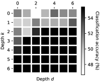
(a) KKI

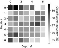
(b) MUTAG

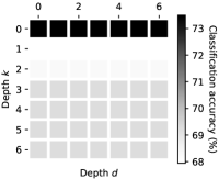
(c) DHFR_MD

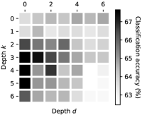
(d) PTC_FM

Figure 4: Parameter sensitivity of MWSP. $d$ represents the depth of the truncated BFS tree rooted at each node which is used for the extraction of shortest paths whose maximal length is $d$. $k$ represents the depth of the truncated BFS tree rooted at each node which is used for capturing multiple different scales of the graph structure around each node (for augmenting graph nodes). Each entry in the heatmap is the mean classification accuracy over the 10-fold.

V Conclusion

In this paper, we have proposed a novel muti-scale graph kernel called MWSP to deal with the two challenges of the R-convolution graph kernels, i.e., they cannot compare graphs at multiple different scales and do not consider the distributions of substructures. To mitigate the first challenge, we propose the shortest-path graph/node feature map, whose element represents the number of occurrences of each shortest path in a graph or around a node. Since the shortest-path graph/node feature map cannot compare graphs at multiple different scales, we incorporate into it the multiple different scales of the graph structure, which are captured by the truncated BFS trees of different depths rooted at each node in a graph. To mitigate the second challenge, we adopt the Wasserstein distance to compute the similarity between the multi-scale shortest-path node feature maps of two graphs. Experimental results show that MWSP outperforms the state-of-the-art graph kernels on most datasets. Since the Wasserstein distance has a high time complexity, we would like to develop an efficient distance measure to compute the similarity between the node feature maps of two graphs in the future.

References

- [1] D. Haussler, “Convolution kernels on discrete structures,” Technical report, Department of Computer Science, University of California at Santa Cruz, Tech. Rep., 1999.
- [2] T. Gärtner, P. Flach, and S. Wrobel, “On graph kernels: Hardness results and efficient alternatives,” in Learning theory and kernel machines. Springer, 2003, pp. 129–143.
- [3] S. V. N. Vishwanathan, N. N. Schraudolph, R. Kondor, and K. M. Borgwardt, “Graph kernels,” Journal of Machine Learning Research, vol. 11, no. Apr, pp. 1201–1242, 2010.
- [4] Z. Zhang, M. Wang, Y. Xiang, Y. Huang, and A. Nehorai, “Retgk: Graph kernels based on return probabilities of random walks,” in NIPS, 2018, pp. 3964–3974.
- [5] K. M. Borgwardt and H.-P. Kriegel, “Shortest-path kernels on graphs,” in International Conference on Data Mining. IEEE, 2005, pp. 8–pp.
- [6] N. Shervashidze, S. Vishwanathan, T. Petri, K. Mehlhorn, and K. Borgwardt, “Efficient graphlet kernels for large graph comparison,” in Artificial Intelligence and Statistics, 2009, pp. 488–495.
- [7] F. Costa and K. D. Grave, “Fast neighborhood subgraph pairwise distance kernel,” in ICML. Omnipress, 2010, pp. 255–262.
- [8] T. Horváth, T. Gärtner, and S. Wrobel, “Cyclic pattern kernels for predictive graph mining,” in SIGKDD. ACM, 2004, pp. 158–167.
- [9] R. Kondor and H. Pan, “The multiscale laplacian graph kernel,” in NIPS, 2016, pp. 2990–2998.
- [10] J. Ramon and T. Gärtner, “Expressivity versus efficiency of graph kernels,” in Proceedings of the first international workshop on mining graphs, trees and sequences, 2003, pp. 65–74.
- [11] P. Mahé and J.-P. Vert, “Graph kernels based on tree patterns for molecules,” Machine learning, vol. 75, no. 1, pp. 3–35, 2009.
- [12] N. Shervashidze and K. M. Borgwardt, “Fast subtree kernels on graphs,” in Advances in neural information processing systems, 2009, pp. 1660–1668.
- [13] N. Shervashidze, P. Schweitzer, E. J. v. Leeuwen, K. Mehlhorn, and K. M. Borgwardt, “Weisfeiler-lehman graph kernels,” Journal of Machine Learning Research, vol. 12, no. Sep, pp. 2539–2561, 2011.
- [14] G. Da San Martino, N. Navarin, and A. Sperduti, “A tree-based kernel for graphs,” in Proceedings of the 2012 SIAM International Conference on Data Mining. SIAM, 2012, pp. 975–986.
- [15] M. Togninalli, E. Ghisu, F. Llinares-López, B. A. Rieck, and K. Borgwardt, “Wasserstein weisfeiler-lehman graph kernels,” Advances in Neural Information Processing Systems 32, vol. 9, pp. 6407–6417, 2020.
- [16] G. Nikolentzos, P. Meladianos, and M. Vazirgiannis, “Matching node embeddings for graph similarity,” in Thirty-first AAAI conference on artificial intelligence, 2017.
- [17] Y. Rubner, C. Tomasi, and L. J. Guibas, “The earth mover’s distance as a metric for image retrieval,” International journal of computer vision, vol. 40, no. 2, pp. 99–121, 2000.
- [18] S. Lazebnik, C. Schmid, and J. Ponce, “Beyond bags of features: Spatial pyramid matching for recognizing natural scene categories,” in 2006 IEEE computer society conference on computer vision and pattern recognition (CVPR’06), vol. 2. IEEE, 2006, pp. 2169–2178.
- [19] K. Grauman and T. Darrell, “The pyramid match kernel: Efficient learning with sets of features.” Journal of Machine Learning Research, vol. 8, no. 4, 2007.
- [20] A. Leman and B. Weisfeiler, “A reduction of a graph to a canonical form and an algebra arising during this reduction,” Nauchno-Technicheskaya Informatsiya, vol. 2, no. 9, pp. 12–16, 1968.
- [21] R. Kondor and T. Jebara, “A kernel between sets of vectors,” in Proceedings of the 20th international conference on machine learning (ICML-03), 2003, pp. 361–368.
- [22] D. J. Watts and S. H. Strogatz, “Collective dynamics of ‘small-world’networks,” nature, vol. 393, no. 6684, pp. 440–442, 1998.
- [23] R. Andersen, F. Chung, and K. Lang, “Local graph partitioning using pagerank vectors,” in 2006 47th Annual IEEE Symposium on Foundations of Computer Science (FOCS’06). IEEE, 2006, pp. 475–486.
- [24] F. Chung, “The heat kernel as the pagerank of a graph,” Proceedings of the National Academy of Sciences, vol. 104, no. 50, pp. 19 735–19 740, 2007.
- [25] A. Gretton, K. M. Borgwardt, M. J. Rasch, B. Schölkopf, and A. Smola, “A kernel two-sample test,” The Journal of Machine Learning Research, vol. 13, no. 1, pp. 723–773, 2012.
- [26] N. Pržulj, D. G. Corneil, and I. Jurisica, “Modeling interactome: scale-free or geometric?” Bioinformatics, vol. 20, no. 18, pp. 3508–3515, 2004.
- [27] T. N. Kipf and M. Welling, “Semi-supervised classification with graph convolutional networks,” International Conference on Learning Representations (ICLR), 2016.
- [28] N. M. Kriege, P.-L. Giscard, and R. Wilson, “On valid optimal assignment kernels and applications to graph classification,” in Advances in Neural Information Processing Systems, 2016, pp. 1623–1631.
- [29] T. H. Schulz, P. Welke, and S. Wrobel, “Graph filtration kernels,” in Proceedings of the AAAI Conference on Artificial Intelligence, 2022.
- [30] T. Mikolov, K. Chen, G. Corrado, and J. Dean, “Efficient estimation of word representations in vector space,” arXiv preprint arXiv:1301.3781, 2013.
- [31] L. Bai, L. Cui, and H. Edwin, “A hierarchical transitive-aligned graph kernel for un-attributed graphs,” in International Conference on Machine Learning. PMLR, 2022, pp. 1327–1336.
- [32] S. S. Du, K. Hou, B. Póczos, R. Salakhutdinov, R. Wang, and K. Xu, “Graph neural tangent kernel: Fusing graph neural networks with graph kernels,” in Advances in Neural Information Processing Systems, 2019.
- [33] A. Jacot, F. Gabriel, and C. Hongler, “Neural tangent kernel: Convergence and generalization in neural networks,” in Advances in neural information processing systems, 2018, pp. 8571–8580.
- [34] S. Arora, S. S. Du, W. Hu, Z. Li, R. Salakhutdinov, and R. Wang, “On exact computation with an infinitely wide neural net,” arXiv preprint arXiv:1904.11955, 2019.
- [35] Y. Tang and J. Yan, “Graphqntk: Quantum neural tangent kernel for graph data,” in Advances in neural information processing systems, 2022.
- [36] A. Figalli and C. Villani, “Optimal transport and curvature,” in Nonlinear PDE’s and Applications. Springer, 2011, pp. 171–217.
- [37] B. Haasdonk and C. Bahlmann, “Learning with distance substitution kernels,” in Joint pattern recognition symposium. Springer, 2004, pp. 220–227.
- [38] G. Loosli, S. Canu, and C. S. Ong, “Learning svm in kreĭn spaces,” IEEE transactions on pattern analysis and machine intelligence, vol. 38, no. 6, pp. 1204–1216, 2015.
- [39] P. Yanardag and S. Vishwanathan, “Deep graph kernels,” in Proceedings of the 21th ACM SIGKDD International Conference on Knowledge Discovery and Data Mining. ACM, 2015, pp. 1365–1374.
- [40] G. Siglidis, G. Nikolentzos, S. Limnios, C. Giatsidis, K. Skianis, and M. Vazirgiannis, “Grakel: A graph kernel library in python,” arXiv preprint arXiv:1806.02193, 2018.
- [41] C.-C. Chang and C.-J. Lin, “Libsvm: a library for support vector machines,” TIST, vol. 2, no. 3, p. 27, 2011.
- [42] K. Kersting, N. M. Kriege, C. Morris, P. Mutzel, and M. Neumann, “Benchmark data sets for graph kernels,” 2016. [Online]. Available: http://graphkernels.cs.tu-dortmund.de
- [43] S. Pan, J. Wu, X. Zhu, G. Long, and C. Zhang, “Task sensitive feature exploration and learning for multitask graph classification,” IEEE transactions on cybernetics, vol. 47, no. 3, pp. 744–758, 2017.
- [44] A. K. Debnath, R. L. Lopez de Compadre, G. Debnath, A. J. Shusterman, and C. Hansch, “Structure-activity relationship of mutagenic aromatic and heteroaromatic nitro compounds. correlation with molecular orbital energies and hydrophobicity,” Journal of medicinal chemistry, vol. 34, no. 2, pp. 786–797, 1991.
- [45] J. J. Sutherland, L. A. O’brien, and D. F. Weaver, “Spline-fitting with a genetic algorithm: A method for developing classification structure- activity relationships,” Journal of chemical information and computer sciences, vol. 43, no. 6, pp. 1906–1915, 2003.
- [46] N. Wale, I. A. Watson, and G. Karypis, “Comparison of descriptor spaces for chemical compound retrieval and classification,” Knowledge and Information Systems, vol. 14, no. 3, pp. 347–375, 2008.
- [47] N. Kriege and P. Mutzel, “Subgraph matching kernels for attributed graphs,” arXiv preprint arXiv:1206.6483, 2012.
- [48] K. M. Borgwardt, C. S. Ong, S. Schönauer, S. Vishwanathan, A. J. Smola, and H.-P. Kriegel, “Protein function prediction via graph kernels,” Bioinformatics, vol. 21, no. suppl_1, pp. i47–i56, 2005.
- [49] P. D. Dobson and A. J. Doig, “Distinguishing enzyme structures from non-enzymes without alignments,” Journal of molecular biology, vol. 330, no. 4, pp. 771–783, 2003.
- [50] N. M. Kriege, M. Fey, D. Fisseler, P. Mutzel, and F. Weichert, “Recognizing cuneiform signs using graph based methods,” in International Workshop on Cost-Sensitive Learning. PMLR, 2018, pp. 31–44.