Abstract

High energy cosmic rays illuminate the Sun and produce an image that could be observed in up to five different channels: a cosmic ray shadow (whose energy dependence has been studied by HAWC); a gamma ray flux (observed at $E\leq 200$ GeV by Fermi-LAT); a muon shadow (detected by ANTARES and IceCube); a neutron flux (undetected, as there are no hadronic calorimeters in space); and a flux of high energy neutrinos. Since these signals are correlated, the ones already observed can be used to reduce the uncertainty in the still undetected ones. Here we define a simple set up that explains the Fermi-LAT and HAWC observations and implies very definite fluxes of neutrons and neutrinos from the solar disk. In particular, we provide a fit of the neutrino flux at 10 GeV–10 TeV that includes its dependence on the zenith angle and on the period of the solar cycle. This flux represents a neutrino floor in indirect dark matter searches. We show that in some benchmark models the current bounds on the dark matter-nucleon cross section push the solar signal below this neutrino floor.

 

1 Introduction

The surface of the Sun is at a temperature $T\approx 0.5$ eV, while its core is burning Hydrogen at $T\approx 1$ keV. Nuclear reactions there produce neutrinos that reach the Earth unscattered with energies of up to 10 MeV. In addition, solar flares are able to accelerate nuclei and electrons up to a couple of GeV. The Sun, however, can also be observed at energies above the GeV. The emission in these other channels is indirect: instead of particles accelerated by the Sun, it appears when high energy cosmic rays (CRs) illuminate its surface. In particular, EGRET [1] and Fermi-LAT [2] (see also [3]) have observed a sustained flux of gamma rays coming from the solar disk that extends up to 200 GeV. The signal, stronger during a solar minimum and interpreted as the albedo flux produced by CRs showering in the Sun’s surface, is ten times above the diffuse gamma-ray background and six times larger than a 1991 estimate by Seckel, Stanev and Gaisser [4]. Obviously, the same mechanism should produce as well neutrinos and neutrons, which are also neutral and thus able to reach the Earth revealing their source.

Although the solar emission of high energy particles induced by CRs was already discussed 40 years ago[4], a precise calculation has been plagued by the uncertainties introduced by the solar magnetism. Here we propose a complete and consistent framework that avoids these difficulties by using the data and implies a clear correlation among the different signals that may be accessible at several astroparticle observatories. If observed, they would provide a multi-messenger picture of the Sun complementary to the one obtained with light and keV-MeV neutrinos.

2 Absorption of cosmic rays

If we point with a detector of CRs to the Sun, we will observe a shadow: the CR shadow of the Sun [5]. Suppose there were no solar magnetism, so that CRs follow straight lines. Then the trajectories aiming to the Earth but absorbed by the Sun would define a black disk of radius $r=0.26^{\circ}$, the angular size of the Sun as seen from the Earth. Indded, this is what we will see at very high energies, when the deflection of CRs by the solar magnetic field is negligible, but not at lower energies. CRs of energy below 100 TeV are very affected by a magnetic field that, unfortunately, is very involved. First of all, it has a radial component (open lines that define the Parker interplanetary field [6]) that grows like $1/R^{2}$ as we approach the surface. This gradient in the field may induce a magnetic mirror effect: CRs approaching the Sun tend to bounce back. In addition, the solar wind induces convection, i.e., CRs are propagating in a plasma that moves away from the Sun and makes it more difficult to reach the surface. Finally, closer to the Sun the magnetic turbulence increases and there appears a new type of field lines that start and end on the solar surface. Hopefully, we can understand the absorption rate of CRs by the Sun with no need to solve these details, just by using the data on its CR shadow together with Liouville’s theorem.

The data is provided by HAWC [7], that has studied the energy-dependence of the CR shadow during a solar maximum. The shadow appears at 2 TeV; it is not a black disk of $r=0.26^{\circ}$ but a deficit that extends into a larger angular region. By integrating it we find that at 2 TeV it accounts for a 6% of a black disk, the deficit grows to a 27% at 8 TeV, and at 50 TeV it becomes a 100% deficit, i.e., a complete solar black disk diluted in a $2^{\circ}$ circle.

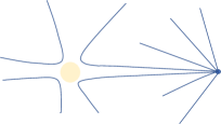
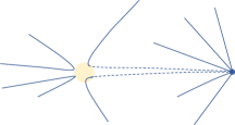
Figure 1: Schematic CR trajectories in the vicinity of the Sun. The solar magnetism does not create anisotropies in the flux reaching the Earth, but the average depth of solar matter crossed by CRs grows with the energy, increasing their probability to be absorbed and thus the integrated CR shadow observed by HAWC.

HAWCs data suggest a simple interpretation based on Liouville’s theorem. The theorem implies that an isotropic CR flux crossing the solar magnetic field will stay isotropic, and that the only possible effect of the Sun is to interrupt some of the trajectories that were aiming to the Earth. As we illustrate in Fig. 1, the solar magnetic field deflects some of the trajectories that were directed to the Earth, but other trajectories will now reach us and the net effect should be zero: an isotropic flux crossing a static magnetic lens, including a mirror, will stay isotropic, and the only possible effect is to create a shadow. At low energies HAWC sees no shadow, meaning that a negligible fraction of the CR flux reaches the solar surface. At higher energies, however, CRs that were supposed to reach the detector hit before the Sun and are absorbed (Fig. 1-right). Therefore, studying the shadow we may deduce the average depth of solar matter crossed by CR’s of different energy in their way to the Earth.

If a CR proton crosses an average depth of $\Delta X_{\rm H}(E)$ the probability to be absorbed is

$$p^{\rm H}_{\rm abs}=1-\exp{\left(-{\Delta X_{\rm H}\over\lambda_{\rm int}^{\rm H}}\right)}\,.$$ (1)

To explain the data we will assume

$${\Delta X_{\rm H}\over\lambda_{\rm int}^{\rm H}}=b_{H}\,E^{1.11}\,,$$ (2)

with $E$ in GeV and a time dependent parameter $b_{H}$ that oscillates between $1.6\times 10^{-5}$ during a solar maximum and $4.8\times 10^{-5}$ during a minimum. Since the trajectory of a CR only depends on its rigidity, He nuclei of twice the energy cross the same average depth and

$$b_{\rm He}={b_{\rm H}\over 2^{1.1}}\,{\sigma_{{\rm He}}(E)\over\sigma_{H}(E/2)}\,.$$ (3)

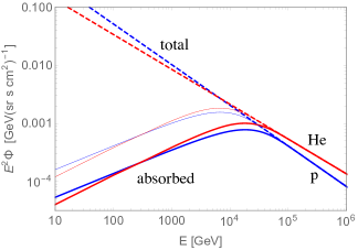
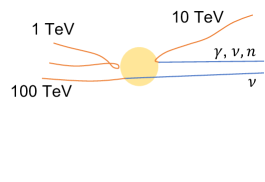
Figure 2: Absorbed proton and He fluxes during a solar maximum (thick) and a solar minimum (thin). On the right, typical CR trajectories at different energies.

In Fig. 2 we plot the CR fluxes from the solar disk that are absorbed at different energies. We have considered a primary CR flux with only proton and He nuclei and slightly different spectral indexs ($-2.7$ and $-2.6$, respectively).

Next we need to model the showering of these absorbed fluxes. A numerical simulation shows that at TeV energies only trajectories very aligned with the open field lines are able to reach the Sun’s surface. Once there, CRs will shower; some of the secondaries will be emitted inwards, towards the Sun, but others will be emitted outwards and may eventually reach the Earth. The probability that a secondary particle contributes to the solar albedo flux will depend on how deep it is produced and in which direction it is emitted.

We assume that secondaries produced by a parent of energy $E$ above some critical energy $E_{\rm c}$ that varies between 6 TeV and 3 TeV for an active or quiet Sun, respectively, will most likely be emitted towards the Sun, whereas lower energy primaries will exit in a random direction:

$$p_{\rm out}={1\over 2}\,\exp\left({E\over E_{\rm c}}\right)^{2}.$$ (4)

Accordingly, we also assume that charged particles of energy below $E_{c}$ are unable to keep penetrating the Sun: they are trapped by closed magnetic lines at the depth where they are produced and shower horizontally.

Under these hypothesis, we use cascade equations [8] to find the final albedo flux of neutral particles (see the complete equations in [9, 10]). The key difference with the usual showers in the Earth’s atmosphere is due to the thin environment where these solar showers develop: below the optical surface of the Sun, it takes 1500 km to cross just 100 g/cm². As a consequence, TeV pions and even muons decay before they loose energy, defining photon and neutrino fluxes well above the atmospheric ones. For neutrinos, to the albedo flux we must add the neutrinos produced in the opposite side of the Sun [11, 12, 13]. Our results for the signal in the different channels are the following.

Figure 3: Gamma ray flux from the solar disk (data from Fermi-LAT [3]).

3 Gamma rays

In Fig. 3 we plot the flux of gamma rays at $E>10$ GeV implied by our set up together with the Fermi-LAT data. This energy flux exhibits two main features. At low energies it is reduced because primary CRs do not reach the Sun; at higher energies it is reduced as well, but because of a different reason: all CRs reach the surface and shower there, but most photons are emitted towards the Sun. Although the set up does not provide a reason for the possible dip at 40 GeV [14], the 400–800 photons per squared meter and year that we obtain seem an acceptable fit of the data.

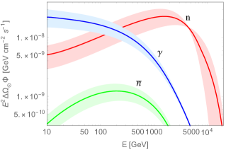
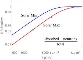
Figure 4: Gamma and neutron fluxes (left) and integrated CR shadow from the solar disk (right); the dots correspond to the HAWC observation [7].

4 Neutrons, CR shadow and muon shadow

Our analysis implies an average of 240 neutrons of energy above 10 GeV reaching the Earth from the solar disk per squared meter and year, with the flux during a solar minimum a factor of 2 larger than during an active phase of the Sun. Most of these neutrons come from the spallation of He nuclei (see Fig. 4-left), resulting in a very characteristic spectrum that peaks at 1-5 TeV. The flux is interesting because neutrons are unstable: they can reach us from the Sun, but not from outside the solar system. In a satellite experiment the background to this solar flux would be the albedo flux from CRs entering the atmosphere, which seems easily avoidable. Unfortunately, space observatories do not carry hadronic calorimeters and are thus unable to detect neutrons.

The solar neutron flux, in turn, has another effect as it enters the atmosphere: it reduces the CR shadow of the Sun measured by HAWC. In Fig. 4-right we give the total shadow (fraction of CRs absorbed by the Sun minus the relative number of neutrons reaching the Earth) predicted by our framework together with HAWC’s data, which was obtained near a solar maximum.

In addition to the CR shadow and the gamma and neutron signals, another interesting channel observable at neutrino telescopes (already detected at ANTARES [15] and IceCube [16]) would be the muon shadow of the Sun when it is above the horizon: down-going muons entering the telescope from the direction of the solar disk. These are muons produced when both the partial shadow of the Sun and the solar neutrons shower in the atmosphere. In Fig. 5 we plot our results as a function of the muon energy (left) or the slant depth at the point of entry in the telescope (right).

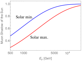
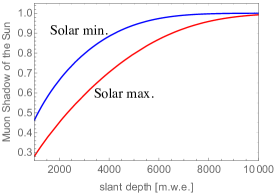
Figure 5: Muon shadow of the Sun at different muon energies (left) or slant depths (right).

The plot for the muon shadow at different slant depths is specially revealing. It compares the number of tracks from the solar disk (smeared into a larger angular region) and from a fake Sun at the same zenith inclination. To observe it in a telescope, one should bin the slant depth of the muon tracks entering the detector and then determine the deficit (integrated to the whole angular region) relative to the fake Sun, finding the fraction of a black disk of $r_{\odot}=0.26^{\circ}$ that it represents. In IceCube [17] the Sun is always very low in the horizon, implying muon tracks of large slant depth and thus always a complete muon shadow of the Sun. KM3NeT [18], however, can access the Sun more vertically and thus from smaller slant depths (down to 3500 m.w.e.), which could establish the energy dependence of this muon shadow.

5 Neutrinos from the solar disk

The neutrino flux reaching a telescope includes three differents components:

1. Neutrinos produced in the Earth’s atmosphere by the partial CR shadow of the Sun. At CR energies above 50 TeV the shadow is complete and this component vanishes, but at lower energies the shadow disappears and this component should coincide with the atmospheric $\nu$ flux.

2. Neutrinos produced in the atmosphere by the solar neutrons reaching the Earth.

3. The neutrinos produced in the solar surface, both the albedo flux and the flux from the opposite side that reaches the Earth after crossing the Sun.

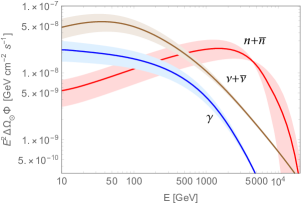
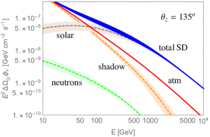
Figure 6: Solar neutrino flux (left) and components defining the neutrino flux observed in a telescope from the solar disk at $\theta_{z}=135^{\circ}$ and atmospheric background at the same zenith inclination (right).

The first two components are absent in all previous analyses. As for the third one, several groups [11, 12, 13] have obtained the neutrino flux produced by CRs showering in the opposite side of the Sun unaffected by the solar magnetic field (see Fig. 2). Their results are larger than ours at energies $E<500$ GeV (in our set up low-energy CRs do not reach the Sun), a $30\%$ smaller at $E\approx 1$ TeV (our albedo flux is not partially absorbed by the Sun in its way to the Earth) and similar at $E>10$ TeV (at high energies neutrinos are produced always inwards). In Fig. 6-left we plot the flux of neutrinos produced in the solar surface together with the albedo flux of gammas and neutrons for comparison. We see that at low energies neutrinos more than double the number of gammas, whereas at $E>5$ TeV all albedo fluxes vanish but we still get the neutrinos produced in the opposite side of the Sun.

In Fig. 6-right we plot the three neutrino components when the Sun is $45^{\circ}$ below the horizon (notice that the fluxes produced by the partial shadow and by the solar neutrons depend on the zenith angle), together with the atmospheric background. The bands express the variation during a solar cicle; the solar and neutron components are larger during a quiet Sun, whereas the $\nu$ component from the partial shadow is larger during a solar maximum. The variation in the total neutrino flux during the 11 year cycle (the blue band in the plot) tends to cancel and is below the 25% at 200 GeV.

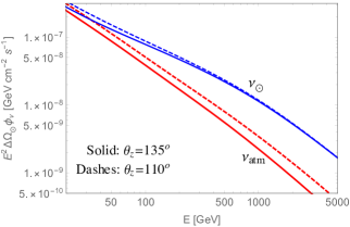
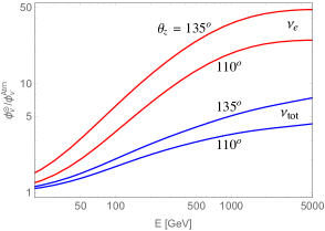
Figure 7: Total neutrino flux from the solar disk versus atmospheric background for the Sun in two different zenith inclinations (left). Signal to background ratio for $\nu_{e}$ and for the sum of all flavors (right).

We see that the total neutrino flux from the solar disk is well above the atmospheric background at $E>100$ GeV. In Fig. 7-left we compare the two fluxes when the Sun is $45^{\circ}$ or $10^{\circ}$ below the horizon; the second inclination is the typical one for the Sun at IceCube. We see that the signal changes little with the zenith angle, whereas the background is significantly larger when the Sun is near the horizon. In the appendix we provide an analytical fit to these components in the neutrino flux, giving the dependence on $\theta_{z}$ and on the period in the solar cycle. In Fig. 7-right we plot the signal to background ratio. Since the neutrinos produced in the Sun reach the Earth with the same frequency for the three flavors, the ratio is obviously much larger for the $\nu_{e}$ than the $\nu_{\mu}$ flavor, and it grows with the energy and with the zenith inclination.

6 Solar neutrino floor in indirect searches

The annihilation of dark matter (DM) particles $\chi$ captured by the Sun may produce a $\nu$ flux that, to be detectable, must be above the solar flux just obtained. Here we would like to show how to estimate the minimum DM–nucleon collision cross section that would be accessible in indirect searches.

Let us assume a DM annihilation cross section large enough to establish an stationary regime where the capture rate is equal to twice the annihilation rate [19]. For illustration, we will consider 3 possible annihilation channels: $\chi\bar{\chi}\to\tau^{+}\tau^{-}$, $\chi\bar{\chi}\to b\bar{b}$ and $\chi\bar{\chi}\to W^{+}W^{-}$. We parametrize the spin-independent (SI) and spin-dependent (SD) DM-nucleon cross sections [20]

$$\sigma_{\chi N}^{\rm SI}={\mu_{N}^{2}\over\pi}\,\left(c_{1}^{N}\right)^{2}\,;\hskip 14.22636pt\sigma_{\chi N}^{\rm SD}={3\mu_{N}^{2}\over 16\pi}\,\left(c_{4}^{N}\right)^{2}\,,$$ (5)

with $N=p,n$ and $\mu_{N}=m_{N}m_{\chi}/(m_{N}+m_{\chi})$. To deduce the elastic cross section with the 6 most abundant solar nuclei (H, He, N, O, Ne, Fe) we use the nuclear response functions in [21]. As it is customary in direct searches, we will take equal proton and neutron SI couplings ($c_{1}^{n}=c_{1}^{p}$) and will only consider the SD coupling of the proton ($c_{4}^{n}=0$).

In our estimate of the capture rate we use the AGSS09 solar model [22] and the SHM⁺⁺ velocity distribution of the galactic DM [23]. We include the thermal velocity for the solar nuclei, which gives a sizeable contribution ($6\%$ increase) in the captures through SD interactions (dominated by Hydrogen). We obtain the neutrino yields after the propagation from the Sun to the Earth for each annihilation channel with DarkSUSY [24].

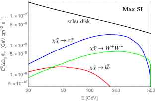
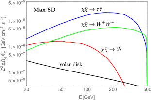
Figure 8: Maximum neutrino flux from DM annihilation consistent with the bounds on $\sigma_{\chi N}^{\rm SI}$ (left) and $\sigma_{\chi N}^{\rm SD}$ (right) from direct searches for the three annihilation channels that we have considered.

To illustrate the reach of DM searches at $\nu$ telescopes, let us fix $m_{\chi}=500$ GeV. For a DM particle that is captured through SI collisions and annihilates into $\tau^{+}\tau^{-}$, a neutrino flux above the solar background established in the previous section requires $\sigma_{\chi N}^{\rm SI}>9.7\times 10^{-46}$ cm². If the annihilation channels are $W^{+}W^{-}$ and $b\bar{b}$ then the elastic cross section must be $\sigma_{\chi N}^{\rm SI}>3.1\times 10^{-45}$ cm² and $\sigma_{\chi N}^{\rm SI}>3.0\times 10^{-44}$ cm², respectively. These cross sections, however, are already excluded by direct searches at XENON1T [25]: $\sigma_{\chi N}^{\rm SI}<4.4\times 10^{-46}$ cm². In Fig. 8 we plot the neutrino fluxes at the Earth for this maximum value of $\sigma_{\chi N}^{\rm SI}$ together with the solar background. The fluxes from DM annihilation are below the solar background in the whole energy range. If DM had only SI interactions with matter, and it had this mass and annihilation channels, indirect searches would reach the solar neutrino floor before they discover it.

Indirect searches could discover DM only if it had monochromatic annihilation channels (e.g., $\chi\bar{\chi}\to\nu X$) or a large SD cross section, which is much less constrained. In particular, PICO-60 establishes that $\sigma_{\chi p}^{\rm SD}<1.8\times 10^{-40}$ cm² at $m_{\chi}=500$ GeV [26], while a DM that annihilates into $W^{+}W^{-}$ requires just $\sigma_{\chi p}^{\rm SD}>1.6\times 10^{-42}$ cm² to be above the flux of solar neutrinos.

7 Summary and discussion

TeV CRs induce an indirect solar emission that was discussed more than 40 years ago and has already been detected in gamma rays. Here we have used the energy dependence of the shadow of the Sun at HAWC to define a set up that implies very definite fluxes of gammas, neutrons and neutrinos. The set up explains the peculiar spectrum of the solar gammas observed at Fermi-LAT’s: low energy CRs do not contribute to the albedo flux as they do not reach the solar surface, whereas high energies CRs reach the Sun, but they produce gammas that are emitted mostly inwards and never reach the Earth. As we discuss in Section 4, our framework could be confirmed if KM3NeT observed a slant-depth dependence in the muon shadow of the Sun. We propose up to five different (but related) signals whose observation would draw a more complete picture of the solar magnetism and of the propagation of TeV CRs near the surface.

The neutrino fluxes from the solar disk are specially interesting, as there is currently an important experimental effort for indirect DM searches. We show that the neutrino fluxes reaching a telescope include three components: (i) the solar emission from both sides of the Sun, (ii) neutrinos produced when the partial CR shadow of the Sun enters the atmosphere, and (iii) neutrinos produced also in the atmosphere by the albedo flux of solar neutrons. The two last contributions have not been discussed in previous literature. In the appendix we provide fits for these components, giving their explicit dependence on the zenith angle and the period of the 11 year solar cycle.

These neutrinos define a floor in DM searches. In particular, we find that the maximum SI elastic cross section consistent with current bounds from XENON1T implies a flux of neutrinos from DM annihilations into $\tau^{+}\tau^{-}$, $b\bar{b}$ or $W^{+}W^{-}$ already below this floor. Therefore, a precise characterization of the $\nu$ fluxes from the solar disk induced by CRs is essential both to decide the optimal detection strategy and to establish the reach of indirect DM searches at each neutrino telescope.

Appendix A Fit to the neutrino fluxes

Here we provide approximate fits for the atmospheric and solar fluxes integrated over the angular region ($\Delta\Omega_{\odot}$, with a radius of $0.26^{\circ}$) occupied by the Sun. In these expressions $E$ is in GeV and $t$ in years ($t=0$ at the solar minimum), whereas $\Delta\Omega_{\odot}\,\Phi_{\nu_{\mu}}^{\rm atm}$ is given in GeV^-1 cm^-2 s^-1. The angle $\theta^{*}(\theta_{z})$ is defined in [27, 28]:

$$\tan\theta^{*}={R_{\oplus}\sin\theta_{z}\over\sqrt{R_{\oplus}^{2}\cos^{2}\theta_{z}+\left(2R_{\oplus}+h\right)h}}\,.$$ (6)

For the atmospheric flux we have

$$\Delta\Omega_{\odot}\,\Phi_{\nu_{\mu}}^{\rm atm}(E,\theta)=1.05\times 10^{3}\;E^{-2.97-0.0108\log E-0.00141\log^{2}E}\,F^{\rm atm}_{1}(E,\theta)\,;$$ (7)

$$\Delta\Omega_{\odot}\,\Phi_{\nu_{e}}^{\rm atm}(E,\theta)=460\;E^{-3.30-0.0364\log^{1.35}E+0.0103\log^{1.85}E}\,F^{\rm atm}_{2}(E,\theta)\,,$$ (8)

with

$$F^{\rm atm}_{1}(E,\theta)={\left({176\over E}\right)^{0.6}+\cos[\theta^{*}({\pi\over 4})]\over\left({176\over E}\right)^{0.6}+\cos[\theta^{*}(\theta_{z})]}\,;\;\;F^{\rm atm}_{2}(E,\theta)={\left({7.5\times 10^{-4}\over E}\right)^{0.21}+\cos[\theta^{*}({\pi\over 4})]\over\left({7.5\times 10^{-4}\over E}\right)^{0.21}+\cos[\theta^{*}(\theta_{z})]}\,.$$ (9)

For the atmospheric neutrinos from both the CR shadow of the Sun and solar neutrons,

$$\Delta\Omega_{\odot}\,\Phi_{\nu_{\mu}}^{\rm shad+n}(E,\theta,t)=1.04\times 10^{3}\;E^{G^{\rm atm}_{1}(E,t)}\,F^{\rm atm}_{1}(E,\theta)\,;$$ (10)

$$\Delta\Omega_{\odot}\,\Phi_{\nu_{e}}^{\rm shad+n}(E,\theta,t)=327\;E^{G^{\rm shad+n}_{2}(E,t)}\,F^{\rm atm}_{2}(E,\theta)$$ (11)

with

$$G^{\rm shad+n}_{1}(E,t)=-2.98-0.017\log E+0.012\cos{2\pi t\over 11}\log^{2}E-3.3\times 10^{-4}\log^{3}E-4.1\times 10^{-6}\log^{5}E\,;$$ (12)

$$G^{\rm shad+n}_{2}(E,t)=-3.1-0.061\log E-\cos{2\pi t\over 11}\left(0.00305\log E+2.1\times 10^{-6}\log^{5}E\right)-5.3\times 10^{-7}\log^{6}E\,.$$ (13)

Finally, the neutrinos produced in the Sun come in the three flavors with the same frequency and

$$\Delta\Omega_{\odot}\,\Phi_{\nu_{i}}^{\rm\odot}(E,t)=\left(1.50-{572\sin^{2}{\pi t\over 11}\over 900+E}\right)E^{-1.20-0.1\log E-0.0042\log^{2}E+1.6\times 10^{-5}\log^{4}E}\,.$$ (14)

References

- [1] E. Orlando and A. W. Strong, Astron. Astrophys. 480 (2008) 847 [arXiv:0801.2178 [astro-ph]].
- [2] A. A. Abdo et al. [Fermi-LAT Collaboration], Astrophys. J. 734 (2011) 116 [arXiv:1104.2093 [astro-ph.HE]].
- [3] T. Linden, B. Zhou, J. F. Beacom, A. H. G. Peter, K. C. Y. Ng and Q. W. Tang, Phys. Rev. Lett. 121 (2018) no.13, 131103 [arXiv:1803.05436 [astro-ph.HE]].
- [4] D. Seckel, T. Stanev and T. K. Gaisser, Astrophys. J. 382 (1991) 652.
- [5] M. Amenomori et al. [Tibet ASgamma], Phys. Rev. Lett. 111 (2013) no.1, 011101 [arXiv:1306.3009 [astro-ph.SR]].
- [6] R. C. Tautz, A. Shalchi and A. Dosch, J. Geophys. Res. Space Phys. 116 (2011) 2102 [arXiv:1011.3325 [astro-ph.HE]].
- [7] O. Enriquez-Rivera et al. [HAWC Collaboration], PoS ICRC 2015 (2016) 099 [arXiv:1508.07351 [astro-ph.SR]].
- [8] T. K. Gaisser, “Cosmic rays and particle physics,” Cambridge, UK: Univ. Pr. (1990) 279 p
- [9] M. Masip, Astropart. Phys. 97 (2018) 63 [arXiv:1706.01290 [hep-ph]].
- [10] C. Gámez, M. Gutiérrez, J. S. Martínez and M. Masip, JCAP 01 (2020), 057 doi:10.1088/1475-7516/2020/01/057 [arXiv:1904.12547 [hep-ph]].
- [11] J. Edsjo, J. Elevant, R. Enberg and C. Niblaeus, JCAP 1706 (2017) 033 [arXiv:1704.02892 [astro-ph.HE]].
- [12] K. C. Y. Ng, J. F. Beacom, A. H. G. Peter and C. Rott, Phys. Rev. D 96 (2017) no.10, 103006 [arXiv:1703.10280 [astro-ph.HE]].
- [13] C. A. Arguelles, G. de Wasseige, A. Fedynitch and B. J. P. Jones, JCAP 1707 (2017) 024 [arXiv:1703.07798 [astro-ph.HE]].
- [14] Q. W. Tang, K. C. Y. Ng, T. Linden, B. Zhou, J. F. Beacom and A. H. G. Peter, Phys. Rev. D 98 (2018) no.6, 063019 [arXiv:1804.06846 [astro-ph.HE]].
- [15] A. Albert et al. [ANTARES], Phys. Rev. D 102 (2020) no.12, 122007 [arXiv:2007.00931 [astro-ph.HE]].
- [16] M. G. Aartsen et al. [IceCube], Phys. Rev. D 103 (2021) no.4, 042005 [arXiv:2006.16298 [astro-ph.HE]].
- [17] A. Achterberg et al. [IceCube Collaboration], Astropart. Phys. 26 (2006) 155 [astro-ph/0604450].
- [18] S. Adrian-Martinez et al. [KM3Net Collaboration], J. Phys. G 43 (2016) no.8, 084001 [arXiv:1601.07459 [astro-ph.IM]].
- [19] G. Jungman, M. Kamionkowski and K. Griest, Phys. Rept. 267 (1996), 195-373 doi:10.1016/0370-1573(95)00058-5 [arXiv:hep-ph/9506380 [hep-ph]].
- [20] A. L. Fitzpatrick, W. Haxton, E. Katz, N. Lubbers and Y. Xu, JCAP 02 (2013), 004 doi:10.1088/1475-7516/2013/02/004 [arXiv:1203.3542 [hep-ph]].
- [21] R. Catena and B. Schwabe, JCAP 04 (2015), 042 [arXiv:1501.03729 [hep-ph]].
- [22] M. Asplund, N. Grevesse, A. J. Sauval and P. Scott, Ann. Rev. Astron. Astrophys. 47 (2009), 481-522 [arXiv:0909.0948 [astro-ph.SR]].
- [23] N. W. Evans, C. A. J. O’Hare and C. McCabe, Phys. Rev. D 99 (2019) no.2, 023012 [arXiv:1810.11468 [astro-ph.GA]].
- [24] T. Bringmann, J. Edsjö, P. Gondolo, P. Ullio and L. Bergström, JCAP 07 (2018), 033 [arXiv:1802.03399 [hep-ph]].
- [25] E. Aprile et al. [XENON], Phys. Rev. Lett. 121 (2018) no.11, 111302 [arXiv:1805.12562 [astro-ph.CO]].
- [26] C. Amole et al. [PICO], Phys. Rev. D 100 (2019) no.2, 022001 [arXiv:1902.04031 [astro-ph.CO]].
- [27] P. Lipari, Astropart. Phys. 1 (1993), 195-227.
- [28] M. Gutiérrez, G. Hernández-Tomé, J. I. Illana and M. Masip, Astropart. Phys. 134-135 (2022), 102646 [arXiv:2106.01212 [hep-ph]].