Vibrational relaxation and triggering of the non-equilibrium vibrational decomposition of CO₂ in gas discharges

Abstract

Non-equilibrium vibrational dissociation of CO₂ at low translational-rotational temperatures $T$ is investigated computationally for conditions of microwave induced plasmas. Semi-analytic treatment of vibrational relaxation in CO₂ in shock tube and acoustic experiments is summarized. A state-to-state vibrational kinetics model applied for the simulations is benchmarked and adjusted to the relaxation times obtained in gas dynamic experiments. The governing parameter $Q/n^{2}_{0}$ has been introduced, where $Q$ is the specific volumetric power coupled in plasma and $n_{0}$ is the initial number density of CO₂. The modelling results indicate a rapid increase of the rate of the primary dissociation process CO₂ + M $\to$ CO + O + M when $Q/n^{2}_{0}$ exceeds some critical value. A simple analytic calculation of $\left(Q/n^{2}_{0}\right)_{crit}$ is proposed which agrees well with the numerical results. At $T$=300 K the estimated $\left(Q/n^{2}_{0}\right)_{crit}\eqsim 6\cdot 10^{-40}$ W$\cdot$m³.

CO₂, vibrational relaxation, dissociation, microwave plasma, plasma conversion

1 Introduction

Plasma chemical conversion of CO₂ into CO is intensively studied now as a potential upstream process for production of synthetic fuels and chemicals (Power-2-X)  [1, 2, 3]. Initially those studies were inspired by, presumably, very high energy efficiency of the CO₂ conversion in microwave plasmas reported in the past [4, 5]. The chemical energy efficiency $\eta_{chem}$ up to 80 % achieved at relatively low translational-rotational temperatures $T\lesssim$1000 K was ascribed to dissociation from high vibrational states in conditions of strong vibrational non-equilibrium [6, 4, 5].

The reported high efficiencies at low $T$ were not reproduced later. In the modern day experiments the highest $\eta_{chem}$ of 40..50 % are observed at $T>$2000 K and are largely explained by thermal quenching [7, 8, 9, 10]. Nevertheless, activating the non-equilibrium conversion mechanism remains an attractive option for increasing the efficiency of plasma processes and making them competitive with electrolysis in this respect. In the present paper a theoretical and numerical evaluation is given of the conditions at which the non-equilibrium process could be triggered.

The most complete computational description of the CO₂ vibrational kinetics and chemistry is provided by the dedicated state-to-state models [11, 12, 13, 14, 15]. Despite their complexity the models developed so far still involve a number of uncertainties and do not allow accurate quantitative predictions. At the same time, as it will be shown here, already on this stage the 0D vibrational kinetics models can be useful in determining the threshold above which the target process could be activated in principle. This threshold is defined in terms of the parameter $Q/n^{2}_{0}$, where $Q$ is the specific (volumetric) power input into electrons, and $n_{0}$ is the initial number density of molecules.

The computational study is performed here with the 2-modes model [15] where the treatment of the CO₂ kinetics is simplified by introducing one effective mode for both kinds of symmetric vibrations. In a series of numerical experiments the rate of the primary dissociation process CO₂ + M $\to$ CO + O + M is shown to rapidly increase starting from zero when $Q/n^{2}_{0}$ is increased above some critical value. This critical value is found to be not sensitive with respect to model uncertainties. Furthermore, the process threshold can be also calculated approximately on the basis of a simple semi-empiric balance equation for vibrational energy which originates from vibrational relaxation studies in shock tube and sound absorption experiments. The threshold determined by the semi-empiric calculation agrees well the results of numerical simulations. The obtained critical value $\left(Q/n^{2}_{0}\right)_{crit}$ can be used for analysis and planning of experiments aiming at achieving the non-equilibrium vibrational mechanism of CO₂ conversion.

Since the rate of vibrational relaxation in CO₂ plays a decisive role in determining the triggering conditions of the non-equilibrium process the first part of the paper focuses specifically on that topic. Section 2 summarizes the analytic and semi-analytic models which describe the relaxation of vibrational energy in CO₂. In section 3 the 2-modes model [15] is benchmarked against the experimental relaxation times of the gas dynamic experiments. It is demonstrated that the model can be adjusted such that the experimental relaxation times are matched. The rest of the paper deals with the main subject of the present work. Section 4 describes the numerical experiments with the calibrated model [15] applied to conditions of microwave induced plasmas. An approximate approach for calculating the critical values of $Q/n^{2}_{0}$ is introduced in section 5, and verified with help of the simulation results. Last section gives a summary of the main findings and a brief outlook on the outstanding issues.

2 Analytic treatment of vibrational relaxation in CO₂

The basic information about vibrational relaxation in molecular gases is obtained in shock tube and acoustic experiments [16, 17, 18]. Here for compactness the consideration is structured around relaxation in shock waves. Same relaxation processes take place in sound waves and the relaxation rates deduced from both types of experiments agree [17, 18]. Behind shock wave fronts a very rapid increase of translational temperature is followed by its fast equilibration with rotational temperature. The characteristic time of translational-rotational relaxation is $\sim$10^-9 sec at atmospheric pressure (see [16], Section 48, 49). The thermal excitation of vibrational states is much slower: the typical characteristic times at 1 bar are 10^-6..10^-5 sec. At the same time, unless the temperatures are not very high, the change of the gas composition due to chemical reactions takes place on a significantly longer time scale.

It is well known that for a gas of diatomic molecules with unchanging number density the relaxation of vibrational energy after instant increase of translational-rotational temperature $T$ can be described by a simple differential equation, see e.g. [16], Chapter 19:

$$\frac{dE_{vibr}}{dt}=\frac{1}{\tau}\left[E^{eq}_{vibr}\left(T\right)-E_{vibr}\right]$$ (1)

Here $E_{vibr}$ is the average specific vibrational energy per molecule, $E^{eq}_{vibr}\left(T\right)$ is the average vibrational energy per molecule at Boltzmann equilibrium with temperature $T$, $\tau$ is the relaxation time which depends only on $T$ and on the number density of molecules $n$:

$$\tau^{-1}=R_{10}\left(T\right)n\left(1-e^{-\frac{\hbar\omega}{T}}\right)$$ (2)

$R_{10}$ is the rate coefficient of transition from the first vibrationally excited state to vibrational ground state, $\hbar\omega$ is the energy of one vibrational quantum. Here and below, unless specified explicitly, the temperatures are always expressed in energy units.

Equations (1), (2) are derived on the following assumptions: i) the molecules are linear (harmonic) oscillators; ii) the probabilities of vibrational-translational (VT) transitions obey the SSH (Schwartz-Slawski-Herzfeld) or Landau-Teller relations; iii) the number of vibrational states is infinite. For CO₂ which has 3 modes of oscillations (1), (2) have to be modified. Two more assumptions are added: iv) exchange of vibrational energy with translational-rotational modes proceeds only via transitions between the bending mode oscillations:

$$CO_{2}\left(v_{1}v^{l}_{2}v_{3}\right)+M\to CO_{2}\left(v_{1},v^{l\pm 1}_{2}\pm 1,v_{3}\right)+M$$ (3)

v) exchange of energy between bending modes and stretching modes is very fast. Rigorous derivation under assumptions above can be found in A. The resulting equation is same as (1), but with $E_{vibr}$ on the right hand side replaced by $E_{vibr-2}$ - the specific vibrational energy per molecule accumulated in bending mode $v^{l}_{2}$ only:

$$\frac{dE_{vibr}}{dt}=R_{10}\left(T\right)n\left(1-e^{-\frac{\hbar\omega_{2}}{T}}\right)\left[E^{eq}_{vibr-2}\left(T\right)-E_{vibr-2}\right]$$ (4)

$$E^{eq}_{vibr-2}\left(T\right)=\frac{2\hbar\omega_{2}}{e^{\frac{\hbar\omega_{2}}{T}}-1}$$ (5)

here $\hbar\omega_{2}$ is the fundamental energy of bending oscillations $v_{2}$. $E^{eq}_{vibr-2}\left(T\right)$ is calculated by applying the known formula for harmonic oscillators, see e.g. [19], equation (49.3) there. Factor 2 takes into account that the mode $v_{2}$ of CO₂ is double degenerate. $R_{01}$ is the rate coefficient of the process:

$$CO_{2}\left(01^{1}0\right)+M\to CO_{2}\left(00^{0}0\right)+M$$ (6)

In [20] it had been shown that when a system of linear oscillators initially has Boltzmann distribution with temperature equal to the translational-rotational temperature $T$, and $T$ is instantly increased, then vibrational relaxation towards final equilibrium state proceeds via a sequence of Bolzmann distributions with vibrational temperature $T_{vibr}\leq T$. The result of [20] is not directly applicable to CO₂, but numerical experiments with state-to-state model [15] presented below in section 3 confirm its validity in that case as well. For the Boltzmann vibrational distribution equation (4) is transformed into equation for $T_{vibr}$ which can be easily integrated:

$$\frac{dT_{vibr}}{dt}=\frac{R_{10}\left(T\right)n\left(1-e^{-\frac{\hbar\omega_{2}}{T}}\right)}{c_{vibr}\left(T_{vibr}\right)}\left[E^{eq}_{vibr-2}\left(T\right)-E^{eq}_{vibr-2}\left(T_{vibr}\right)\right]$$ (7)

Here $c_{vibr}\left(T_{vibr}\right)=\frac{dE_{vibr}}{dT_{vibr}}$ is the (dimensionless) heat capacity due to vibrational modes which is calculated by using the formulas for linear oscillators, see e.g. [19], equation (49.4):

$$c_{vibr}\left(T_{vibr}\right)=c_{1}+2c_{2}+c_{3},\quad c_{i}=\frac{\left(\hbar\omega_{i}\right)^{2}e^{\frac{\hbar\omega_{i}}{T_{vibr}}}}{T^{2}_{vibr}\left(e^{\frac{\hbar\omega_{i}}{T_{vibr}}}-1\right)^{2}}$$ (8)

$\hbar\omega_{i}$ are the fundamental energies of the 3 modes of CO₂ oscillations.

The assumption of Bolzmann distribution of vibrational levels allows to derive one more equation where the rate of vibrational relaxation appears explicitly - by transforming (4) into equation for $E_{vibr-2}$:

$$\frac{dE_{vibr}}{dt}=\frac{dE_{vibr}}{dE_{vibr-2}}\frac{dE_{vibr-2}}{dt}=\frac{\frac{dE_{vibr}}{dT_{vibr}}}{\frac{dE_{vibr-2}}{dT_{vibr}}}\frac{dE_{vibr-2}}{dt}=\frac{c_{vibr}\left(T_{vibr}\right)}{2c_{2}\left(T_{vibr}\right)}\frac{dE_{vibr-2}}{dt}$$

$$\frac{dE_{vibr-2}}{dt}=\frac{2c_{2}\left(T_{vibr}\right)}{c_{vibr}\left(T_{vibr}\right)}R_{10}\left(T\right)n\left(1-e^{-\frac{\hbar\omega_{2}}{T}}\right)\left[E^{eq}_{vibr-2}\left(T\right)-E_{vibr-2}\right]$$ (9)

One can see that the rate of relaxation (subsequently, the instant relaxation time) is not independent of $T_{vibr}$, but this dependency is weak. The factor $\frac{2c_{2}}{c_{vibr}}$ only changes from 1 at low $T_{vibr}$ where $c_{2}\gg c_{1},\,c_{3}$ (because $\hbar\omega_{2}<\hbar\omega_{1},\,\hbar\omega_{3}$) to $\frac{2c_{2}}{c_{vibr}}=\frac{1}{2}$ at high $T_{vibr}$ where $c_{1},\,c_{2},\,c_{3}\to 1$.

Equation (9) suggests the following approximation. One can assume that the total vibrational energy $E_{vibr}$ decays with exactly same rate as $E_{vibr-2}$, and then apply equation (1) with $\tau$ defined as:

$$\tau^{-1}=\frac{2c_{2}\left(\bar{T}\right)}{c_{vibr}\left(\bar{T}\right)}R_{10}\left(T\right)n\left(1-e^{-\frac{\hbar\omega_{2}}{T}}\right)$$ (10)

Here $\bar{T}$ is some average temperature, e.g. $\bar{T}=\frac{1}{2}\left(T_{0}+T\right)$ where $T_{0}$ is the initial Boltzmann temperature before the vibrational relaxation starts. Of note is that a relation similar to (10) appears also in [17], equation (24) there.

To estimate the accuracy of this approximation a comparison is made with numerical solution of equation (7) with constant $T$. Both solutions are expressed in terms of the dimensionless time:

$$t^{\prime}=t\cdot R_{10}\left(T\right)n\left(1-e^{-\frac{\hbar\omega_{2}}{T}}\right)$$ (11)

That is, the explicit dependence on $n$ and $R_{10}$ is eliminated. The temperature $T_{vibr}$ obtained by solving (7) is translated into $E_{vibr}$ by the linear oscillator formula:

$$E_{vibr}\left(T_{vibr}\right)=\frac{\hbar\omega_{1}}{e^{\frac{\hbar\omega_{1}}{T_{vibr}}}-1}+\frac{2\hbar\omega_{2}}{e^{\frac{\hbar\omega_{2}}{T_{vibr}}}-1}+\frac{\hbar\omega_{3}}{e^{\frac{\hbar\omega_{3}}{T_{vibr}}}-1}$$ (12)

The fundamental energies of the CO₂ oscillations [21]: $\hbar\omega_{1}$=0.16783 eV, $\hbar\omega_{2}$=0.083427 eV, $\hbar\omega_{3}$=0.29710 eV. The time evolution $E_{vibr}\left(t^{\prime}\right)$ is compared with the exponential function:

$$E^{\tau}_{vibr}\left(t\right)=E_{vibr}\left(T\right)+\left[E_{vibr}\left(T_{0}\right)-E_{vibr}\left(T\right)\right]e^{-t/\tau}$$ (13)

where $t$ is replaced by $t^{\prime}$ and $\tau$ is replaced by $\tau^{\prime}=\frac{c_{vibr}\left(\bar{T}\right)}{2c_{2}\left(\bar{T}\right)}$, see (10) and (11). The relative difference $\epsilon$ between two solutions is defined as:

$$\epsilon=\max_{t^{\prime}}{\left[\frac{\left|E_{vibr}\left(t^{\prime}\right)-E^{\tau}_{vibr}\left(t^{\prime}\right)\right|}{E_{vibr}\left(t^{\prime}\right)}\right]}$$ (14)

where the maximum is taken over the time interval from $t^{\prime}=0$ to $t^{\prime}=10\cdot\tau^{\prime}$.

For the test with $T_{0}$=300 K and $\bar{T}=\frac{1}{2}\left(T_{0}+T\right)$ the quantity $\epsilon$ is found to be always $\leq$5 % for $T\leq$2500 K. This outcome means that, provided that all the assumptions underlying (7) are fulfilled, the time evolution of $E_{vibr}$ can be approximated with good accuracy by equation (1) with $\tau$ defined by (10). This characteristic time, in turn, depends on the rate coefficient of only one process (6). The coefficient $R_{10}$ then serves as a single parameter which fits the vibrational kinetics model into experimental data. It will be shown in the next section that this result holds as well when equation (7) is replaced by state-to-state simulations.

3 Benchmark of the CO₂ vibrational kinetics for conditions of gas-dynamic experiments

The equations introduced the previous section can be used to calibrate a state-to-state model of the CO₂ vibrational kinetics such that it reproduces the experimental relaxation times in a situation which mimics conditions behind a shock front. This will be demonstrated here with the so called ’2-modes’ model described in [15]. This is a coarse-grained model where elementary vibrational states $CO_{2}\left(v_{1}v^{l}_{2}v_{3}\right)$ are gathered into ’combined’ symmetric-asymmetric states $CO_{2}\left[v_{s},v_{a}\right]$; $v_{a}=v_{3}$, and $v_{s}=2v_{1}+v_{2}$ is a good quantum number which combines symmetric stretching and bending modes. The model includes dissociation of CO₂ from the ’unstable’ states with vibrational energies exceeding the dissociation limit of 5.5 eV. The rates of vibrational transitions between combined states are calculated by applying scalings based mainly on the Herzfeld (SSH) theory [22]. The absolute values of the rate coefficients of transitions between symmetric and asymmetric modes are adjusted to the laser florescence data. The same applies to vibrational-vibrational (VV) transitions between asymmetric modes, the rates of VV-transitions between symmetric modes are purely theoretical. Adjustment (calibration) of the rates of vibrational-translational (VT) transfer (3) is discussed below.

The experimental data on VT-transfer in CO₂ had been commonly published in form of relaxation times $\tau$ defined in terms of equation (1). The experimental $\tau$s could be reduced to functions of translational-rotational temperature $T$ only [17, 18]. The most recent review found on the subject is the publication [23]. By comparing that paper with the older report [24] one finds no references on process (3) with M=CO₂ which had not been taken into account in [24]. Therefore, here the rate coefficient of process (6) as a function of $T$ is taken from [24] (process $\left(01^{1}0\right)\to\left(00^{0}0\right)$, M=CO₂, in Table IIIa there) as the best fit of the all available experimental data. Apparently, this rate coefficient was obtained by applying equation (2) with $\hbar\omega=\hbar\omega_{2}$ rather than equation (10). The correctness of this assumption is confirmed by translating the rate coefficient back into $\tau\left(T\right)$, and comparing the result with selected primary publications on the relaxation time measurements. This comparison is shown in figure 1 where $\tau\left(T\right)$ ’reverse engineered’ as described above (’Blauer-Nickerson 1973’) is plotted together with results of the shock tube [25, 18] and sound absorption [26, 27] experiments. The agreement is very good.

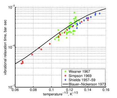
Figure 1: Experimental characteristic time of vibrational relaxation $\tau$, see equation (1), at pressure 1 bar. ’Weaner 1967’ is [25], ’Simpson 1969’is [18] ’Shields 1967-59’ is [26, 27] as reproduced in [18]. Solid line is the fit from [24]

The rate coefficient of process (6) applied here is calculated by using equation (10) with $\tau$ derived from the rate coefficient $R^{BN73}_{10}$ of that process in [24]. That is:

$$R_{10}\left(T\right)=\frac{c_{vibr}\left(\bar{T}\right)}{2c_{2}\left(\bar{T}\right)}R^{BN73}_{10}\left(T\right),\quad\bar{T}=\frac{1}{2}\left(300\;{\rm K}+T\right)$$ (15)

The coefficient $R^{BN73}_{10}$ corrected in that way can be fitted by the equation:

$$R_{10}\left(T\right)=4.48\cdot 10^{-13}\exp{\left(-198.8T^{-1/3}+517.6T^{-2/3}\right)}$$ (16)

Here $T$ is in Kelvin and the resulting $R_{10}$ is in m³/s. For $T$ from 250 K to 2000 K (16) approximates (15) with maximum relative deviation 0.5 %. The magnitude of the correction factor was already discussed in section 2: the original and corrected rate coefficients are nearly equal at low $T$, and $R_{10}$ is twice as large as $R^{BN73}_{10}$ at high $T$ ($\geq$2000 K). The rate coefficients of the transitions from higher excited states are obtained from $R_{10}$ by applying SSH scaling as described in [15].

The 2-modes model is benchmarked by applying the same test problem as in the previous section. Initial gas has Boltzmann vibrational distribution with $T_{0}$=300 K, the temperature $T>T_{0}$ is prescribed and fixed. The system relaxes by thermal excitation of vibrational states until the equilibrium vibrational distribution is reached which corresponds to the temperature $T$. For $T\leq$2500 K considered here the change of the CO₂ number density due to dissociation on the time-scale of the test is in all cases $<$0.01 %.

In a very general sense a state-to-state model can be written as initial value problem for the set of ordinary differential equations:

$$\frac{dn_{k}}{dt}=\sum_{i,j}a^{k}_{ij}n_{i}n_{j}$$ (17)

Where $n_{k}$, $n_{i}$, $n_{j}$ are the number densities of individual species - excited states, and coefficients $a^{k}_{ij}$ are functions of the temperature $T$ only . It can be easily shown that changing of the gas pressure $p$ at fixed $T$ does not change the shape of the solution of (17). Indeed, replacing densities with concentrations $c$: $n_{k}=c_{k}n_{0}$, where $n_{0}$ is the total initial density of molecules, yields :

$$\frac{1}{n_{0}}\frac{dc_{k}}{dt}=\sum_{i,j}a^{k}_{ij}c_{i}c_{j}$$

The solution of this equation written in terms of $n_{0}t$ - the integration time scaled proportional to $n_{0}$ - depends only on $T$. Therefore, all the reference model runs here are made for one nominal pressure $p$=1 bar. Two test with $p$=0.1 bar and $p$=10 bar yield, as expected, exactly same results within relative difference 10^-7 when the time-traces $E_{vibr}\left(n_{0}t\right)$ are compared.

The time evolution of specific vibrational energy $E_{vibr}$ calculated by the 2-modes model is compared with exponential function (13) with $\tau$ defined by (10). To remind, since $R_{10}$ is defined by (15) this $\tau$ is the fit of the primary experimental data. Selected time-traces of $E_{vibr}$ are shown in figure 2. One can see a very good agreement up to $T$=1500 K, the agreement deteriorates at higher temperatures. Quantitative comparison of the numerical solution and the analytic formula is given in table 1 in terms of relative deviation $\epsilon$ defined by (14). The meaning of the parameter $p^{max}_{SSH}$ will be explained below. One can see that for $T\leq$1500 K the exponential function fits the numerical solution within 4 %. That is, the conclusion on the applicability of the simple formula (10) made in the previous section is confirmed by a state-to-state model. Or, the other way around, the test demonstrates that in conditions which mimic those behind a shock front the state-to-state model calibrated as prescribed by equation (10) yields at $T\leq$1500 K (to some extent up to 2000 K) the same relaxation behavior as the empiric equation (1).

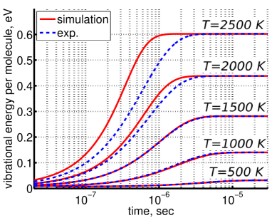
Figure 2: Comparing the time evolution of vibrational energy $E_{vibr}$ in the test problem of section 3 simulated by the 2-modes model [15] (solid lines) and approximated by the exponential function (13) with $\tau$ defined by (10) (dashed lines). $T$ is the fixed translational-rotational temperature

Table 1: Comparison of $E_{vibr}\left(t\right)$ in the test problem of section 3 simulated by the 2-modes model [15] and approximated by (13), (10) in terms of the relative error $\epsilon$ defined by (14)

	$p^{max}_{SSH}$=1		$p^{max}_{SSH}$=0.1
$T$, K	$\epsilon$, %	$\eta_{V1}$ %	$\epsilon$, %	$\eta_{V1}$ %
350	0.2 (0.2)	100.0	0.2	100.0
400	0.6 (0.5)	99.9	0.6	99.9
500	1.6 (1.5)	99.8	1.6	99.8
600	2.6 (2.6)	99.6	2.6	99.6
800	3.9 (3.9)	98.9	3.9	98.9
1000	4.0 (4.0)	97.7	4.0	97.7
1200	3.1 (3.2)	95.5	3.1	95.5
1500	1.0 (0.6)	89.6	1.0	89.6
2000	12.2 (10.4)	71.9	12.2	72.0
2500	31.9 (28.4)	48.7	31.3	50.3

The numerical simulations allow to verify the assumptions behind the equations (7) and (10). In particular, of the linear oscillators assumption which is only applied in the 2-modes model for calculation of matrix elements of transitions. The vibrational energies are calculated with the full anharmonic expression [21]. To estimate the importance of anharmonicity the simulations were repeated with energies calculated in linear (harmonic) approximation. The resulting values of $\epsilon$ are shown in the second column of table 1 in parentheses, the difference in the outcome of the benchmark is negligible.

The most non-obvious assumption underlying the derivation of (7) is that of the dominance of transition (3) in the thermal excitation of vibrational energy. For its verification in 2-modes calculations the relative contribution of process (3) in the total energy exchange is calculated:

$$\eta_{V1}=\frac{\int_{t}Q_{V1}\left(t\right)dt}{\int_{t}Q_{tot}\left(t\right)dt}$$

here $Q_{tot}\left(t\right)$ is the total power transferred from translational-rotational to vibrational modes, $Q_{V1}\left(t\right)$ is the power transferred by the process (3) only, the integral is calculated over the whole time interval where the equations are solved. One can see from table 1 that $\eta_{V1}\geq$90 % for $T\leq$1500 K, and this is exactly the temperature range where the agreement between the 2-modes simulations and the semi-empiric fit is good. Above 2000 K the assumption of the dominance of (3) does not hold any more, and the relaxation equations of section 2 are not applicable. At high $T$ the transfer of translational-rotational energy into vibrational modes is taken over by inter-mode transitions $CO_{2}\left(v_{1},v^{l}_{2},v_{3}\right)+M\to CO_{2}\left(u_{1},u^{m}_{2},v_{3}\pm 1\right)+M$ (processes V2 in [15]). At $T\geq$3000 K this is the dominant mechanism of thermal excitation of vibrational energy. This conclusion drown for high temperatures has to be taken with caution because besides the shortcomings of the SSH scaling which will be discussed below the absolute values of the rate coefficients of the inter-mode transitions applied in the present model are based on the laser fluorescence data available only for $T\leq$1000 K.

The SSH theory [22] applied in 2-modes model [15] to scale the probabilities of vibrational transitions from low to high excited states is a first order perturbation theory. It is known that this theory can grossly overestimate the transition probabilities for very high excited states and at high temperatures. To cope with that issue in the model the transition probabilities treated by the SSH theory are not allowed to be larger than the prescribed parameter $p^{max}_{SSH}$. The nominal value of this parameter is 1. In order to check the influence of $p^{max}_{SSH}$ the test of the present section was repeated with $p^{max}_{SSH}$=0.1. The results are shown in the two last columns of table 1. The difference is only visible starting from $T$=2000 K, and does not affect the conclusions drawn above.

The shortcoming of the SSH theory is solved in the non-perturbative Forced Harmonic Oscillators (FHO) model [28]. Recently, FHO calculations of the probabilities of vibrational transitions in CO₂ became available [29, 30, 31]. A comparison between the rate coefficients $R$ of VT-transition (3) calculated by the SSH and FHO methods has shown that the FHO correction has only a small impact on the calculated rate of that process. This comparison was performed for the set of the FHO rate coefficients of the transitions:

$$CO_{2}\left(0v_{2}^{v_{2}}0\right)+M\to CO_{2}\left(0\left(v_{2}-1\right)^{v_{2}-1}0\right)+M,\quad M=CO_{2}$$ (18)

taken from [31], file K_CO2v2_CO2_VT.mat, following the description in [30]. The SSH calculations are described in [15, 32], the vibrational energies of the molecules are calculated according to [21]. The rate coefficients of selected transitions calculated by the two models are plotted in figure 3. Both SSH and FHO calculations are normalized such that for $v_{2}$=1 the rate coefficient equals to that of the process $\left(01^{1}0\right)\to\left(00^{0}0\right)$ in Table IIIa of [24]. One can see that in the temperature range from 300 to 1500 K the deviation between SSH and FHO scalings is small. For $v_{2}\leq$10 which corresponds to total vibrational energy of the molecule $\leq$0.84 eV the relative difference $\epsilon_{SSH}=\left|R_{FHO}-R_{SSH}\right|/R_{FHO}$ is always $\leq$12 %. The upper boundary of $\epsilon_{SSH}$ is increased for higher $v_{2}$, e.g. for $v_{2}$=20 (energy 1.70 eV) $\epsilon_{SSH}\leq$20 %, but even for the highest level $v_{2}$=63 (energy 5.54 eV) $\epsilon_{SSH}$ stays smaller than 32 %.

The FHO model also allows to calculate the probabilities of multi-quantum transitions which are not accounted for in first order perturbation theories. Comparison between the rate coefficients of the single-quantum transitions (18) and the corresponding two-quantum rates in the data set [31] shows that at room temperature $T$=300 K the two-quantum transitions are always by more than a factor 100 less probable. The importance of multi-quantum transitions is increased at higher $T$. However, the ratio $R_{1-q}/\left(2R_{2-q}\right)$ - where $R_{1-q}$ is the rate of a single-quantum transition, and $R_{2-q}$ is the rate of the two-quantum transition from the same $v_{2}$ - stays $>$10 at $T\leq$1000 K even for the largest $v_{2}$=63 ($>$5 at $T\leq$1500 K). With decreasing $v_{2}$ the ratio $R_{1-q}/\left(2R_{2-q}\right)$ is increased.

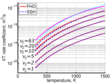
Figure 3: Rate coefficients of the process (18) taken from the set of FHO calculations  [29, 30, 31] (solid lines) compared with the coefficients calculated according to the SSH theory [22]

For transitions other than (3), in particular for vibrational-vibrational (VV) transfer, the difference between FHO and SSH scalings can be much large. As has been shown above, at $T<$2000 K those other transitions are relatively unimportant for thermal excitation of vibrational energy. At the same time, the inter-mode and VV transitions (see [15], Table 1 there) are the processes which govern fast energy exchange between different kinds of vibrational modes and bring them to Boltzmann distribution with single temperature $T_{vibr}$. Although the absolute values of their coefficients are adjusted to experimental data the SSH scaling can lead to very inaccurate values for high excited states. Nevertheless, as long as those processes in the model are fast enough this inaccuracy may not have large impact on the final result. Strong coupling between different types of vibrations in the 2-modes simulations agrees with the fact that in shock tube experiments only one or two very close relaxation times were detected [17, 18].

4 Simulation of the non-equilibrium vibrational dissociation of CO₂ in microwave plasmas

The model [15] with vibrational relaxation rate benchmarked as described in the previous section is applied to investigate the onset of the non-equilibrium vibrational dissociation in CO₂. The same approach to modelling of the electron impact excitation of vibrational states as in [15] is adopted here with one important modification. Instead of degree of ionization the total specific (volumetric) power input $Q$ into electrons is prescribed and fixed in a model run. In practice this means that the electron density $n_{e}$ is calculated as:

$$n_{e}=\frac{Q}{\sum_{i}R_{ei}E_{i}n_{i}}$$ (19)

where $n_{i}$ is the number density of molecular species (excited state) $i$, $R_{ei}$ is the total rate coefficient of all the electron impact processes with species $i$, and $E_{i}$ is the energy transferred on average from electrons in each collision with $i$.

The set of master equations solved by the model in the discharge zone $Q>0$ can be written in the same form as (17) with the electron excitation term added:

$$\frac{dn_{k}}{dt}=\sum_{i,j}a^{k}_{ij}\left(T\right)n_{i}n_{j}+\sum_{i}R^{k}_{ei}\left(T_{e}\right)n_{e}n_{i}$$

Substituting (19) and introducing concentrations $c_{k}$: $n_{k}=c_{k}n_{0}$ and the Specific Energy Input (SEI) per one initial molecule $\epsilon=Qt/n_{0}$ brings the equations above to the form:

$$\frac{dc_{k}}{d\epsilon}=\frac{n^{2}_{0}}{Q}\sum_{i,j}a^{k}_{ij}\left(T\right)c_{i}c_{j}+\frac{\sum_{i}R^{k}_{ei}\left(T_{e}\right)c_{i}}{\sum_{i}R_{ei}\left(T_{e}\right)E_{i}\left(T_{e}\right)c_{i}}$$ (20)

The coefficients $R_{ei}$, $R^{k}_{ei}$, $E_{i}$ are functions of the electron temperature $T_{e}$. As one can see from (20) for the constant $T$ and $T_{e}$ the solution expressed in terms of $c_{i}$ and $\epsilon$ depends only on the parameter $Q/n^{2}_{0}$.

The rate coefficients $R_{ei}$ are calculated here assuming the maxwellian electron energy distribution which is approximately valid for conditions of microwave induced plasmas, see [33, 34, 12]. A more accurate calculation of the energy distribution function was considered to be superfluous since no excited state resolved data are readily available for the electron impact transitions anyway, thus, only a very basic model of those processes is applied. Only one quantum transitions are taken into account and same rate coefficients are applied for all excited states, see [15]. The modelling studies with detailed electron kinetics [34, 12] have shown that in conditions of microwave plasmas at not too low pressures the kinetic energy acquired by electrons predominantly goes into vibrational excitations. The results of [12] suggest that this statement is valid at least at 20 Torr. Therefore, for this kind of gas discharges the quantity $Q$ of the present model which does not include the power spent to any other kinds of electron processes (such as dissociation or ionization) can be taken as approximately equal to the total power coupled in plasma. The electron temperature $T_{e}$=1 eV used in the reference simulations here reflects the typical average electron energy calculated for conditions in question.

The outcome of the model calculations for selected fixed temperatures $T$ are shown in figure 4. The results are presented in terms of $Q/n^{2}_{0}$ and the ’process rate’ $\chi$ defined as the fraction of initial CO₂ molecules which dissociate in the process CO₂ + M $\to$ CO + O + M. For all model runs this quantity is taken at the time instants which correspond to $\epsilon$=3 eV:

$$\chi=1-\frac{n_{CO_{2}}\left(\epsilon=3~{}{\rm eV}\right)}{n_{CO_{2}}\left(\epsilon=0\right)}$$ (21)

Conversion in the afterglow ($Q$=0) is not taken into account since in the previous work [15] the conversion on that phase was found to be insignificant. The chosen final value of $\epsilon$ is close to the net enthalpy change of the total process CO₂ $\to$ CO + $\frac{1}{2}$O₂ $\Delta H_{f}$=2.93 eV which is the ideal cost of producing one CO molecule. That is, $\epsilon$ which is larger than that value will lead to inevitable losses of energy not into the target process even at 100 % conversion of CO₂ into CO.

The CO₂ kinetics model applied for simulations here is incomplete in terms of chemistry - it does not include the secondary processes with O-atoms and reverse reactions. Also, interaction of CO₂ with reaction products CO, O₂, O is not taken into account. Therefore, the calculated $\chi$ is not expected to be a quantitatively correct prediction, but rather an indication that the process has been started. At the same time, the model can be considered as valid in the vicinity of the threshold values of $Q/n^{2}_{0}$ there the total CO₂ conversion is yet low and the influence of products on the primary dissociation process is expected to be small. That is, the determination of the $Q/n^{2}_{0}$ threshold above which efficient dissociation from high vibrational states can start is the main result of the simulations, not the absolute values of $\chi$ at higher $Q/n^{2}_{0}$.

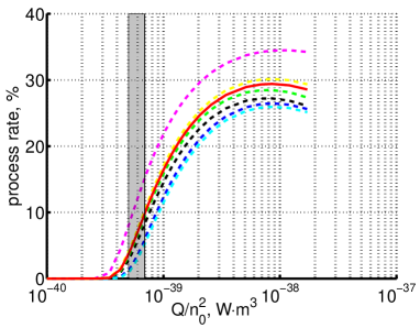
(a) $T$=300 K

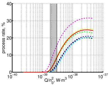
(b) $T$=500 K

(c) $T$=800 K

Figure 4: ’Process rate’ $\chi$ defiend by (21) as a function of parameter $Q/n^{2}_{0}$, see equation (20), calculated by the 2-modes model [15] for fixed translational-rotational temperature $T$. Solid line is the reference model, dashed lines are the simulations with uncertain parameters varied, see section 4. Shaded rectangles is the approximate calculation of $\left(Q/n^{2}_{0}\right)_{crit}$, section 5

All the simulations presented in figure 4 are technically performed for the nominal pressure $p$=100 mbar. To confirm that, as suggested by (20), there is no explicit pressure dependence the calculations were repeated with different values of $p$. The relative differences of $\chi$ calculated with $p$=50 mbar and $p$=200 mbar and those at $p$=100 mbar for the same values of $Q/n^{2}_{0}$ (only $\chi>$0.1 % are taken into account) are found to be always $<$0.7 %.

The solid lines in figures 4 present the solutions obtained with the reference model, and the dashed lines are the results of the simulations where the model uncertainties are evaluated. The issue that the SSH theory can grossly overestimate transition probabilities has been already discussed in section 3. The potential impact of that shortcoming of the SSH scaling is estimated by reducing the imposed upped boundary of the SSH probabilities $p^{max}_{SSH}$ from the reference value 1 to 0.1. The resulting effect is visible although relatively small for $T$=300 K, but tend to increase at higher $T$. Next, because of too large scattering of experimental data the pure theoretical rate coefficients are used for vibrational-vibrational transitions between symmetric modes - they are calculated by the Herzfeld theory [22]. Experience shows that this theory is especially bad in predicting the absolute values of transition probabilities. Therefore, the consequences of reducing or increasing those coefficients had to be evaluated. This is done in the same way as in [15]: the rate coefficients of the all corresponding transitions are multiplied by a factor $f^{s}_{VV}$. Its reference value is 1, $f^{s}_{VV}$=10^-2, 10^-1, 10 are tested. One can see, figure 4, a relatively large modification of the solution, especially when $f^{s}_{VV}$ is increased. At the same time, one can also say that both the variations of $p^{max}_{SSH}$ and $f^{s}_{VV}$ - although they have substantial impact on the steepness of the $\chi$ increase with increased $Q/n^{2}_{0}$ - have a very limited effect on the threshold value of this parameter.

Finally, the effect of changing the electron temperature $T_{e}$ was investigated. In the reference model ($T_{e}$=1 eV) 69..81 % of $Q$ is deposited into asymmetric modes. Two model runs have been added with $T_{e}$=0.5 eV and 2 eV. In the first case the fraction of $Q$ which goes into asymmetric modes is slightly increased up to 80..92 %, in the second case it is reduced down to 57..70 %. As one can see in figure 4 those variations have negligible impact on the solution.

5 Approximate calculation of the process threshold $\left(Q/n^{2}_{0}\right)_{crit}$

The critical value of the parameter $Q/n^{2}_{0}$ above which the non-equilibrium vibrational dissociation may be triggered can be calculated approximately on the basis of the simple considerations which will be put forward below. In the most general terms the balance of vibrational energy of the CO₂ molecules is written as:

$$\frac{d\left(nE_{vibr}\right)}{dt}=Q-Q_{VT}-Q_{diss}$$ (22)

where $n$ is the molecule number density, $E_{vibr}$ is the average vibrational energy per molecule, $Q$ is the power deposited into vibrational modes, $Q_{VT}$ is the rate of the energy losses into translational-rotational modes, and $Q_{diss}$ is the rate of vibrational energy losses into chemical transformations. For the dissociation from the upper vibrational states to be significant their population has to be high enough, that is, $E_{vibr}$ has to be increased up to a certain high value. For this to happen at low translational-rotational temperature $T$ the right hand side of (22) has to be larger than zero.

In the near threshold regimes where $Q_{diss}<Q_{VT}$ the last term can be neglected, and the term $Q_{VT}$ can be written in the form suggested by equation (1):

$$Q_{VT}\left(T,E_{vibr}\right)=R_{VT}\left(T\right)n_{M}n\left[E_{vibr}-E^{eq}_{vibr}\left(T\right)\right]$$ (23)

Where $n_{M}$ is the number density of the collision partners M in the VT-transfer process  (3) - here they are CO₂ molecules too, $R_{VT}\left(T\right)$ is the empiric energy relaxation rate coefficient obtained from the experimental characteristic times $\tau$, see section 3. In practice the coefficient $R_{VT}\left(T\right)$ can be calculated backward from the rate coefficients $R_{10}\left(T\right)$ of process (6) published in the literature:

$$R_{VT}\left(T\right)=R_{10}\left(T\right)\left(1-e^{-\frac{\hbar\omega_{2}}{T}}\right)$$ (24)

as discussed in section 3.

Equation (23) describes vibrational relaxation in gas dynamic experiments and, strictly speaking, must not be valid for the gas discharge conditions. In order to verify to which extent (23) is applicable in that latter case too the magnitude of the term $Q_{VT}$ as it appears in numerical simulations of section 4 is compared directly with that calculated by (23). Examples of this comparison are shown in figure 5. Instead of $E_{vibr}$ the $Q_{VT}$ are plotted as functions of the more illustrative quantity $T_{vibr}$. To translate the simulated $E_{vibr}$ into $T_{vibr}$ equations (A.2) and (A.3) from [15] are used, $E_{vibr}$ in (23) is calculated as a function of $T_{vibr}$ by applying (12). The $R_{VT}\left(T\right)$ in (23) is calculated by using (24), with $R_{10}$ taken from [24]. To remind, the 2-modes model [15] applied for the simulations is adjusted to match the experimental rates of vibrational relaxation which correspond to exactly this choice of $R_{VT}\left(T\right)$, see section 3.

One can see in figure 5 that the agreement is relatively good. This statement is quantified by examining the ratio of $Q_{VT}\left(T_{vibr}\right)$ taken from the simulations and $Q_{VT}\left(T_{vibr}\right)$ obtained with (23). For $T$=300..600 K this ratio always lies between 0.4 and 1.5. These maximum and minimum are taken over the all modelling runs of section 4 including those with varied $T_{e}$, $p^{max}_{SSH}$ and $f^{s}_{VV}$ (only points with $T_{vibr}>T$+100 K are considered). For higher $T$ the upper boundary (maximum) of the ratio above is increased: up to 2.4 for $T$=800 K and up to 3.4 for $T$=1000 K. Nonetheless, even in those cases (23) can always be taken as a good order of magnitude estimate. This is an expected result since vibrational distribution function of the lower vibrational levels in the gas discharge simulations was found to be close to Boltzmann, see an example in [15]. The populations of the upper levels near the dissociation limit deviate strongly from the Boltzmann distribution. However, since their populations are relatively small the high energy tail they form has no overwhelming impact on the total energy exchange rate.

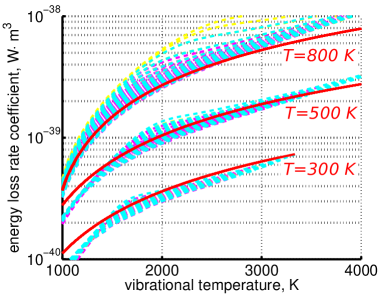
Figure 5: Rate of vibrational energy losses $Q_{VT}$, see (22), divided by $n_{M}n$. Solid line is the result of the approximate formula (23), dashed lines are $Q_{VT}/\left(n_{M}n\right)$ taken from numerical simulations of section 4. Only modelling runs with the process rate $\chi<$12 % are plotted

At constant $T$ the term (23) monotonically increases with increased $E_{vibr}$ so that with $Q_{diss}$=0 the solution of (22) would finally arrive at some required stationary value $E^{*}_{vibr}$ determined by the equality $Q=Q_{VT}\left(T,E^{*}_{vibr}\right)$. Since only the very beginning of the conversion process is considered it can be taken that $n=n_{M}=n_{0}$, where $n_{0}$ is the initial value before the process starts. Then the threshold (critical) value of $Q/n^{2}_{0}$ which corresponds to certain $E^{*}_{vibr}$ is readily found as:

$$\left(\frac{Q}{n^{2}_{0}}\right)_{crit}=R_{VT}\left(T\right)\left[E^{*}_{vibr}-E^{eq}_{vibr}\left(T\right)\right]$$ (25)

The criterion (25) has a simple physics meaning. For the vibrationally non-equilibrium process to start the rate of producing the vibrationally excited states has to be at least as fast as the rate with which vibrational energy is transferred into translational-rotational modes.

The critical $E^{*}_{vibr}$ (or $T^{*}_{vibr}$) which enters (25) can be determined from the condition that at this $T^{*}_{vibr}$ the dissociation term $Q_{diss}$ starts to be comparable with $Q_{VT}$, e.g. by assuming $Q_{diss}\left(T,T^{*}_{vibr}\right)=0.1Q_{VT}\left(T,T^{*}_{vibr}\right)$. Unlike $Q_{VT}$ there is no simple way of calculating $Q_{diss}\left(T,T^{*}_{vibr}\right)$, in particular because the dissociation proceeds from the non-Boltzmann high energy tail of vibrational distribution. Therefore, the determination of $T^{*}_{vibr}$ shall rely on the results of numerical simulations. The model uncertainties lead to a relatively large scattering of that quantity, but, as it will be seen below, this scattering has only minor impact on the final result.

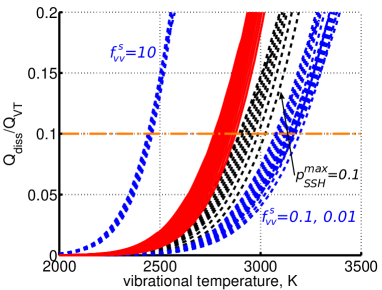
(a) $T$=300 K

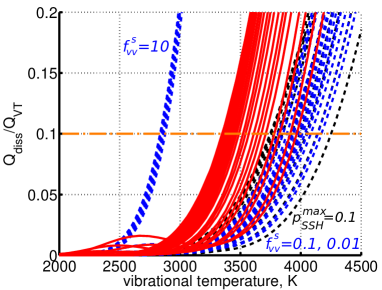
(b) $T$=500 K

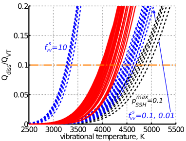
(c) $T$=800 K

Figure 6: Ratio of the $Q_{diss}$ and $Q_{VT}$ terms, equation (22), as function of $T_{vibr}$ in numerical simulations of section 4. Solid lines correspond to the reference model with different values of $T_{e}$. Dashed lines are the cases with $p^{max}_{SSH}$=0.1 and $f^{s}_{VV}$=10^-2, 10^-1, 10. Only modelling runs with the process rate $\chi<$25 % are plotted

Table 2: Semi-empiric estimate of the critical value of $Q/n^{2}_{0}$, see section 5

$T$, K	$T^{*}_{vibr}$, K	$\left(Q/n^{2}_{0}\right)_{crit}$, W$\cdot$m3
300	2500..3200	(5..7)$\cdot$10-40
500	2900..4300	(2..3)$\cdot$10-39
800	3300..5000	(6..11)$\cdot$10-39

The ratio $Q_{diss}\left(T_{vibr}\right)/Q_{VT}\left(T_{vibr}\right)$ obtained in the simulations of section 4 is plotted for selected $T$ in figure 6. The maximum and minimum of $T_{vibr}$ which correspond to $Q_{diss}\left(T_{vibr}\right)/Q_{VT}\left(T_{vibr}\right)\approx 0.1$ for each $T$ are quoted in table 2. The numbers are rounded off because no high accuracy is required here. The corresponding values of $\left(Q/n^{2}_{0}\right)_{crit}$ are obtained by applying equation (25) with $E^{*}_{vibr}\left(T^{*}_{vibr}\right)$ calculated using (12). One can see that the variation of $\left(Q/n^{2}_{0}\right)_{crit}$ caused by the uncertainty of $T^{*}_{vibr}$ is not large. The increase of this parameter with increased $T$ is mainly due to increase of $R_{VT}\left(T\right)$ rather than the term in $[...]$ in (25).

The range of $\left(Q/n^{2}_{0}\right)_{crit}$ from table 2 is shown as shaded rectangles in figures 4. The agreement with the process threshold as it appears in the results of the simulation runs is very good. That is, equation (25) together with the approximate values of $T^{*}_{vibr}$ provided in table 2 can be used as a practical criterion of activation of the non-equilibrium vibrational dissociation of CO₂. The accuracy of this approximate formula in determining the process threshold is not worse than the accuracy provided by a complicated vibrational kinetics model.

6 Summary and outlook

In the present paper activation of the non-equilibrium vibrational dissociation of CO₂ at low translational-rotational temperatures $T$ in microwave gas discharges is investigated by means of computational and semi-empiric models. A series of simulations has been performed with the 2-modes state-to-state model [15]. The model has been benchmarked and adjusted against vibrational relaxation data from the shock tube and acoustic experiments. The governing parameter $Q/n^{2}_{0}$ has been introduced, where $Q$ is the volumetric specific power coupled in plasma, and $n_{0}$ is the initial number density of CO₂. The simulations indicate a rapid increase of the rate of the primary dissociation process CO₂ + M $\to$ CO + O + M with increased $Q/n^{2}_{0}$ when the governing parameter exceeds some critical (threshold) value. The solutions are found to be sensitive with respect to variation of the uncertain model parameters. However, the position of the process threshold as it appears in the simulation results is relatively stable. A simple analytic estimate of the critical value $\left(Q/n^{2}_{0}\right)_{crit}$ based on the experimental rates of vibrational relaxation has been proposed which agrees well with the modelling results.

This estimate provides $\left(Q/n^{2}_{0}\right)_{crit}$=6$\cdot$10^-40 W$\cdot$m³ (averaged) at $T$=300 K. The numerical experiments suggest that within variation of the modelling result no non-equilibrium vibrational process is possible when $Q/n^{2}_{0}<0.5\left(Q/n^{2}_{0}\right)_{crit}$. Efficient conversion of CO₂ into CO by the non-equilibrium process can be expected when $Q/n^{2}_{0}$ is larger than $\left(Q/n^{2}_{0}\right)_{crit}$ withing an order of magnitude, see figure 4a. For completeness it is worth to remind that in case it is applied e.g. for planning of experiments the $Q/n^{2}_{0}$ criterion is to be always supplemented by the straightforward Specific Energy Input (SEI) per molecule consideration. In experiments this quantity is typically controlled by the flow rate. SEI has to be at least larger than the energy per CO₂ molecule which corresponds to the target vibrational temperature $T_{vibr}$: e.g. for $T_{vibr}$=3000 K this is 0.8 eV. At the same time, SEI can not be allowed to be much larger than the net enthalpy change of the transition CO₂ $\to$ CO + $\frac{1}{2}$O₂ $\Delta H_{f}$=2.93 eV because all the energy in excess of $\Delta H_{f}$ can not go into the target reaction.

Formally, it may appear that the parameter $\left(Q/n^{2}_{0}\right)_{crit}$ can be easily increased by decreasing $n_{0}$ - that is, by reducing the gas pressure. In reality the pressure is restricted from below by at least two factors which were not taken into account in the present work. The models applied here always implicitly assume optically thick gas. This assumption can be violated at very low pressures. In that case a one more channel of vibrational energy losses via spontaneous emission will appear in addition to collisional vibrational relaxation. Second, at low pressures the shape of the energy distribution of electrons may shift towards higher energies, and the power coupled in plasma will not go predominantly into vibrational excitations. The kinetic energy of electrons will be rather spent on other kinds of processes, such as direct electron impact dissociation. Proper account of the radiation transport and electron kinetics are two separate topics which were left completely out of the scope of the present work. Models which couple self-consistently the non-maxwellian electron kinetics and the CO₂ vibrational kinetics and chemistry do exist [34, 12]. Their main weakness is that the cross sections of the electron processes with vibrational states of CO₂ are not known to a high degree of accuracy.

The state-to-state model of the present paper is applicable only near the $Q/n^{2}_{0}$ threshold there the rate of conversion via the primary process CO₂ + M $\to$ CO + O + M is not yet too high. In order to further extend its applicability the secondary reactions with oxygen, reverse processes, reaction products and their influence on vibrational kinetics must be added. It can be expected that such extensions will not significantly affect the position of $\left(Q/n^{2}_{0}\right)_{crit}$, but they might have a large impact on the steepness of the conversion rate growth with increased $Q/n^{2}_{0}$.

Adding CO to the model can be seen as a pure technical matter since all the data and models for calculation of the transition rate coefficients are readily available. Adding the oxygen chemistry, on the opposite, can face large difficulties because of the exchange reaction CO₂ + O $\to$ CO + O₂. Too little is known about the influence of vibrational non-equilibrium on that process. To which exactly extent vibrational excitation of CO₂ speeds up this reaction? The process has a relatively low enthalpy change, where the vibrational energy of CO₂ will then go? Will it go into vibrational energy of the products or into their translational-rotational energy? Those questions have no definitive answers. The energy efficiency of the overall conversion process CO₂ $\to$ CO + $\frac{1}{2}$O₂ can be larger than 50 % only if the reaction CO₂ + O $\to$ CO + O₂ is faster than the 3-body recombination O + O + M $\to$ O₂ + M, and if vibrational energy of CO₂ which takes part in the former goes predominantly into the products vibrational energy. It is unlikely that all the unknowns will be resolved in the near future. Therefore, the most realistic next step in the state-to-state modelling studies of the CO₂ vibrational kinetics and chemistry is thought to be a model of a CO₂/CO mixture without oxygen. Particular questions this model could address are the effectiveness of vibrational coupling between CO₂ and CO, effective speed of vibrational relaxation of the mixture and the impact of CO on the primary dissociation process.

Data availability

Link to the archive of the raw output of the modelling runs:
https://doi.org/10.26165/JUELICH-DATA/IHO9NP
The up-to-date source code of the numerical model (Fortran):
https://jugit.fz-juelich.de/reacflow/co2-20

Appendix A Derivation of vibrational relaxation equation for CO₂

Derivation of the equation which describes thermal excitation of vibrational energy in diatomic molecules can be found in [16], Chapter 19. Here the derivation of [16] is modified for CO₂ which has 3 modes of oscillation $v_{1}$, $v_{2}$, $v_{3}$. The mode $v_{2}$ is double degenerate and has rotational momentum $l$: $v^{l}_{2}$. It is assumed that the molecules are linear (harmonic) oscillators and their vibrational energy $E_{v}$ can be expressed as:

$$E_{v}=\hbar\omega_{1}v_{1}+\hbar\omega_{2}v_{2}+\hbar\omega_{3}v_{3}$$

Further assumptions are that vibrational-translational (VT) transfer takes place only from the mode $v^{l}_{2}$ via process (3), and the number of vibrational states is infinite.

Since in the linear oscillator approximation $E_{v}$ does not depend on $l$ all states with same $v_{2}$ can be gathered into a combined state. There are $v_{2}+1$ different values of $l$ possible for a fixed $v_{2}$. The normalized matrix elements $X$ of all possible VT-transitions from the mode $v^{l}_{2}$ are summarized in [32], see equation (27) there:

$$X_{v^{l}_{2}\to\left(v_{2}-1\right)^{l+1}}=v_{2}-l;\quad X_{v^{l}_{2}\to\left(v_{2}-1\right)^{l-1}}=v_{2}+l$$

$$X_{v^{l}_{2}\to\left(v_{2}+1\right)^{l+1}}=v_{2}+l+2;\quad X_{v^{l}_{2}\to\left(v_{2}+1\right)^{l-1}}=v_{2}-l+2$$

The averaged probability $p$ of transition between combined states $v_{2}$ and $v_{2}-1$ calculated by the first order perturbation theory (SSH) is proportional to:

$$p_{v_{2}\to v_{2}-1}\sim\frac{\sum_{l}\left(X_{v^{l}_{2}\to\left(v_{2}-1\right)^{l+1}}+X_{v^{l}_{2}\to\left(v_{2}-1\right)^{l-1}}\right)}{\sum_{l}1}\sim v_{2}$$ (26)

The sum $\sum_{l}$ is taken over all values of $l$ allowed for the corresponding $v_{2}$. Same for the transition between combined states $v_{2}$ and $v_{2}+1$:

$$p_{v_{2}\to v_{2}+1}\sim\frac{\sum_{l}\left(X_{v^{l}_{2}\to\left(v_{2}+1\right)^{l+1}}+X_{v^{l}_{2}\to\left(v_{2}+1\right)^{l-1}}\right)}{\sum_{l}1}\sim v_{2}+2$$ (27)

Some transitions which appear in the sums are not possible. For example the transition from $v_{2}^{v_{2}}$ to $\left(v_{2}-1\right)^{v_{2}+1}$ is not possible because this latter state does not exist. Such transitions must not be excluded explicitly from the sums because the formulas for $X$ automatically give zero in those cases.

Taking into account the assumption that only VT-transitions between modes $v^{l}_{2}$, process (3), are possible the particle balance equations for the number densities $n$ of the combined vibrational states $\left(v_{1},v_{2},v_{3}\right)$ read as follows:

$$\frac{dn_{v_{1}v_{2}v_{3}}}{dt}=k_{v_{2}+1\to v_{2}}n_{v_{1}v_{2}+1v_{3}}+k_{v_{2}-1\to v_{2}}n_{v_{1}v_{2}-1v_{3}}-$$

$$-\left(k_{v_{2}\to v_{2}-1}+k_{v_{2}\to v_{2}+1}\right)n_{v_{1}v_{2}v_{3}},\quad v_{2}>0$$ (28)

$$\frac{dn_{v_{1}0v_{3}}}{dt}=k_{10}n_{v_{1}1v_{3}}-k_{01}n_{v_{1}0v_{3}}$$ (29)

Here $k$ are the transition rates: transition rate coefficients multiplied by the total density of particles M in the process (3). The coefficients $k_{10}$ and $k_{01}$ are connected by the detailed balance relation:

$$\frac{k_{01}}{k_{10}}=\frac{w_{1}}{w_{0}}\exp{\left(-\frac{E_{1}-E_{0}}{T}\right)}=2\exp{\left(-\frac{\hbar\omega_{2}}{T}\right)}=2K$$ (30)

Here $w_{j}$ is the degeneracy of the vibrational level $\left(0,j,0\right)$ which is equal to $j+1$, and $E_{j}$ is its vibrational energy.

All the other rate coefficients in (28), (29), can be connected with $k_{10}$ using the expressions (26), (27) and (30):

$$k_{v_{2}\to v_{2}-1}=v_{2}k_{10},\quad k_{v_{2}\to v_{2}+1}=\left(v_{2}+2\right)Kk_{10}$$ (31)

$$k_{v_{2}+1\to v_{2}}=\left(v_{2}+1\right)k_{10},\quad k_{v_{2}-1\to v_{2}}=\left(v_{2}+1\right)Kk_{10}$$ (32)

Equations (31), (32) are substituted into equations (28), (29). For convenience of notation indexes $v_{1}$, $v_{2}$, $v_{3}$ are replaced by $i$, $j$, $k$ respectively. The resulting master equations read:

$$\frac{dn_{ijk}}{dt}=k_{10}\left(j+1\right)n_{ij+1k}+k_{10}K\left(j+1\right)n_{ij-1k}-$$ (33)

$$-k_{10}jn_{ijk}-k_{10}K\left(j+2\right)n_{ijk},\quad j>0$$

$$\frac{dn_{i0k}}{dt}=k_{10}n_{i1k}-2Kk_{10}n_{i0k}$$ (34)

To obtain the energy relaxation equation the (33) and (34) are multiplied by:

$$E_{v}=\hbar\omega_{1}i+\hbar\omega_{2}j+\hbar\omega_{3}k=E_{ik}+\hbar\omega_{2}j$$

and then their sum over indexes $i$, $j$, $k$ is calculated. This sum reads:

$$\frac{d\left[\sum^{\infty}_{i,j,k=0}\left(E_{ik}+\hbar\omega_{2}j\right)n_{ijk}\right]}{dt}=$$ (35)

$$=k_{10}\hbar\omega_{2}\sum^{\infty}_{i,k=0}\sum^{\infty}_{j=1}\left\{j\left(j+1\right)n_{ij+1k}-j^{2}n_{ijk}+Kj\left(j+1\right)n_{ij-1k}-Kj\left(j+2\right)n_{ijk}\right\}+$$

$$+k_{10}E_{ik}\sum^{\infty}_{i,k=0}\left[\sum^{\infty}_{j=1}\left\{\left(j+1\right)n_{ij+1k}-jn_{ijk}+K\left(j+1\right)n_{ij-1k}-K\left(j+2\right)n_{ijk}\right\}+n_{i1k}-2Kn_{i0k}\right]$$

The second term in (35) equals zero. Indeed, combining the terms without $K$ in the innermost sum yields:

$$\sum^{\infty}_{j=1}\left[\left(j+1\right)n_{ij+1k}-jn_{ijk}\right]+n_{i1k}=\left|j^{\prime}=j+1\right|=$$

$$=\sum^{\infty}_{j^{\prime}=2}j^{\prime}n_{ij^{\prime}k}+n_{i1k}-\sum^{\infty}_{j=1}jn_{ijk}=\sum^{\infty}_{j=1}jn_{ijk}-\sum^{\infty}_{j=1}jn_{ijk}=0$$

Same for the terms with factor $K$:

$$\sum^{\infty}_{j=1}\left[\left(j+1\right)n_{ij-1k}-\left(j+2\right)n_{ijk}\right]-2n_{i0k}=\left|j^{\prime}=j-1,\;j=j^{\prime}+1\right|=$$

$$=\sum^{\infty}_{j^{\prime}=0}\left(j^{\prime}+2\right)n_{ij^{\prime}k}-\sum^{\infty}_{j=1}\left(j+2\right)n_{ijk}-2n_{i0k}=\sum^{\infty}_{j=0}\left(j+2\right)n_{ijk}-\sum^{\infty}_{j=0}\left(j+2\right)n_{ijk}=0$$

The sum:

$$\sum^{\infty}_{i,j,k=0}\left(E_{ik}+\hbar\omega_{2}j\right)n_{ijk}=E_{vibr}n,\quad n=\sum^{\infty}_{i,k,j=0}n_{ijk}$$

is the total specific (per unit volume) vibrational energy; $E_{vibr}$ is the specific vibrational energy per molecule, $n$ is the total number density of molecules. The whole equation (35) is reduced to the following form:

$$\frac{d\left(nE_{vibr}\right)}{dt}=k_{10}\hbar\omega_{2}\sum^{\infty}_{i,k=0}\sum^{\infty}_{j=1}\left[j\left(j+1\right)n_{ij+1k}-j^{2}n_{ijk}\right]+$$

$$+k_{10}\hbar\omega_{2}K\sum^{\infty}_{i,k=0}\sum^{\infty}_{j=1}\left[j\left(j+1\right)n_{ij-1k}-j\left(j+2\right)n_{ijk}\right]$$ (36)

Calculation of the first sum of (36):

$$\sum^{\infty}_{j=1}\left[j\left(j+1\right)n_{ij+1k}-j^{2}n_{ijk}\right]=\left|j^{\prime}=j+1,\;j=j^{\prime}-1\right|=$$

$$=\sum^{\infty}_{j^{\prime}=1}\left(j^{\prime}-1\right)j^{\prime}n_{ij^{\prime}k}-\sum^{\infty}_{j=1}j^{2}n_{ijk}=\sum^{\infty}_{j=1}\left[\left(j-1\right)j-j^{2}\right]n_{ijk}=-\sum^{\infty}_{j=0}jn_{ijk}$$

Calculation of the second sum of (36):

$$\sum^{\infty}_{j=1}\left[j\left(j+1\right)n_{ij-1k}-j\left(j+2\right)n_{ijk}\right]=\left|j^{\prime}=j-1,\;j=j^{\prime}+1\right|=\sum^{\infty}_{j^{\prime}=0}\left(j^{\prime}+1\right)\left(j^{\prime}+2\right)n_{ij^{\prime}k}-$$

$$-\sum^{\infty}_{j=0}j\left(j+2\right)n_{ijk}=\sum^{\infty}_{j=0}\left[\left(j+1\right)\left(j+2\right)-j\left(j+2\right)\right]n_{ijk}=\sum^{\infty}_{j=0}\left(j+2\right)n_{ijk}$$

Substituting the calculated sums back into (36) yields:

$$\frac{d\left(nE_{vibr}\right)}{dt}=k_{10}\hbar\omega_{2}\left[K\sum^{\infty}_{i,k,j=0}\left(j+2\right)n_{ijk}-\sum^{\infty}_{i,k,j=0}jn_{ijk}\right]=$$

$$=k_{10}n\left[KE_{vibr-2}+2\hbar\omega_{2}K-E_{vibr-2}\right]$$ (37)

where:

$$\sum^{\infty}_{i,k,j=0}\hbar\omega_{2}jn_{ijk}=nE_{vibr-2}$$

is the total vibrational energy stored in the mode $v^{l}_{2}$, $E_{vibr-2}$ is its specific value per molecule. Transforming the right hand side of (37) and substituting $K$, equation (30), yields finally:

$$\frac{d\left(nE_{vibr}\right)}{dt}=k_{10}n\left[2\hbar\omega_{2}K-\left(1-K\right)E_{vibr-2}\right]=k_{10}n\left(1-K\right)\left[\frac{2\hbar\omega_{2}K}{1-K}-E_{vibr-2}\right]=$$

$$=k_{10}n\left(1-e^{-\frac{\hbar\omega_{2}}{T}}\right)\left[\frac{2\hbar\omega_{2}}{e^{\frac{\hbar\omega_{2}}{T}}-1}-E_{vibr-2}\right]$$

For $n=const$ and with $k_{10}$ replaced by $R_{10}\left(T\right)n$ this equation gives (4), (5).

References

- [1] Snoeckx R and Bogaerts A 2017 Chem. Soc. Rev. 46 5805
- [2] Bogaerts A and Neyts E C 2018 ACS Energy Letters 3 1013
- [3] van Rooij G J, Akse H N, Bongers W A and van de Sanden M C M 2018 Plasma Phys. Contr. Fusion 60 014019
- [4] Legasov V A et al. 1978 Dokl. Akad. Nauk. 238 66
- [5] Rusanov V D, Fridman A A and Sholin G V 1981 Sov. Phys.-Usp. 24 447
- [6] Capezzuto P, Cramarossa F, d’Agostino R and Molinari E 1976 J. Phys. Chem. 80 882
- [7] Goede A et al. 2014 EPJ Web of Conferences 79 01005
- [8] Bongers W et al. 2017 Plasma Process Polym. 14
- [9] den Harder N et al. 2017 Plasma Process Polym. 14
- [10] D’Isa F A, Carbone E A D, Hecimovic A and Fantz U 2020 Plasma Sources Sci. Tehnol. 29 105009
- [11] Kozak T and Bogaerts A 2014 Plasma Sources Sci. Technol 23 045004
- [12] Pietanza L D, Colonna D and Capitelli M 2020 Phys. Plasmas 27 023513
- [13] Armenise I and Kustova E V 2018 J. Phys. Chem. A 122 5107
- [14] Kunova O, Kosareva A, Kustova E and Nagnibeda E 2020 Phys. Rev. Fluids 5 123401
- [15] Kotov V 2021 Plasma Sources Sci. Technol 30 055003
- [16] Herzfeld K F and Litovitz T A 1959 Absorption and dispersion of ultrasonic waves (New York: Academic Press)
- [17] Taylor R L and Bitterman S 1969 Rev. Mod. Phys. 41 26
- [18] Simpson C J S M, Chandler T R D and Strawson A C 1969 J. Chem. Phys. 51 2214
- [19] Landau L and Lifshitz M 1980 Course of Theoretical physics, vol. 5, Statistical physics. Part 1 (Butterworth-Heinemann)
- [20] Montroll E W and Shuler K E 1957 J. Chem. Phys. 26 454
- [21] Teffo J L, Sulakshina O N and Perevalov V I 1992 J. Mol. Spectr. 156 48
- [22] Herzfeld K F 1967 J. Chem. Phys. 47 743
- [23] Joly V and Robin A 1999 Aerospace Science and Technology 4 229
- [24] Blauer J A and Nickerson G R 1973 Technical report AFRPL-TR-73-57
- [25] Weaner D, Roach J F and Smith W R 1967 J. Chem. Phys. 47 3096
- [26] Shields F D 1957 J. Acoust. Soc. Am. 29 450
- [27] Shields F D 1959 J. Acoust. Soc. Am. 31 248
- [28] Adamovich I V, Macheret S O, Rich J W and Treanor C E 1998 J. Chem. Phys. 12 57
- [29] Vargas J, Lopez B and Lino d S M 2021 J. Phys. Chem. A 125 493
- [30] Lino d S M, Vargas J and Loureiro J 2018 Stellar co2 version 2: A database for vibrationally-specific excitation and dissociation rates for carbon dioxide Report on ESA Contract No. 4000118059/16/NL/KML/fg “Standard Kinetic Models for CO2 Dissociating Flow”
- [31] http://esther.ist.utl.pt/stellar/, retrieved on January 22, 2021
- [32] Kotov V 2020 J. Phys. B 53 175104
- [33] Silva T, Britun N, Godfroid T and Snyders R 2014 Plasma Sources Sci. Tehnol. 23 025009
- [34] Capitelli M, Colonna G, D’Ammando G and Pietanza L D 2017 Plasma Sources Sci. Technol. 26 055009