Tale of GRB 171010A/SN 2017htp and GRB 171205A/SN 2017iuk: Magnetar origin?

Abstract

We present late-time optical follow-up observations of GRB 171010A/SN 2017htp ($z$ = 0.33) and low-luminosity GRB 171205A/SN 2017iuk ($z$ = 0.037) acquired using the 4K$\times$4K CCD Imager mounted at the 3.6m Devasthal Optical Telescope (3.6m DOT) along with the prompt emission data analysis of these two interesting bursts. The prompt characteristics (other than brightness) such as spectral hardness, $T_{\rm 90}$, and minimum variability time-scale are comparable for both the bursts. The isotropic $X$-ray and kinetic energies of the plateau phase of GRB 171205A are found to be less than the maximum energy budget of magnetars, supporting magnetar as a central engine powering source. The new optical data of SN 2017htp and SN 2017iuk presented here, along with published ones, indicate that SN 2017htp is one of the brightest and SN 21017iuk is among the faintest GRB associated SNe (GRB-SNe). Semi-analytical light-curve modelling of SN 2017htp, SN 2017iuk and only known GRB associated superluminous supernova (SLSN 2011kl) are performed using the MINIM code. The model with a spin-down millisecond magnetar as a central engine powering source nicely reproduced the bolometric light curves of all three GRB-SNe mentioned above. The magnetar central engines for SN 2017htp, SN 2017iuk, and SLSN 2011kl exhibit values of initial spin periods higher and magnetic fields closer to those observed for long GRBs and H-deficient SLSNe. Detection of these rare events at such late epochs also demonstrates the capabilities of the 3.6m DOT for deep imaging considering longitudinal advantage in the era of time-domain astronomy.

1 Introduction

Gamma-Ray Bursts (GRBs) are short and highly energetic flashes of radiation occurring at cosmological distances and exhibit non-thermal spectra peaking in the $\gamma$-ray band (Meegan et al., 1992; Band et al., 1993; Kumar & Zhang, 2015; Pe’er, 2015). Due to their high intrinsic luminosities, GRBs are observable up to very high redshifts (z $\sim$8-10). Thus, these are among the potential candidates for increasing our understanding of high-energy physical mechanisms (Mészáros, 2013), probing the properties of the primordial universe (Fiore, 2001; Fynbo et al., 2007) and measuring the cosmological parameters (Amati & Della Valle, 2013; Moresco et al., 2022). Along with many observed prompt emission properties, bursts with $T_{\rm 90}$ duration less than 2s are termed as short/hard GRBs (sGRBs), while those last for more than 2s are designated as long/soft GRBs (lGRBs), see Kouveliotou et al. (1993a); Zhang et al. (2012). Recently, a few ultra-long GRBs (ulGRBs) have also been detected, lasting much longer (a few hundred seconds to hours) in $\gamma$-rays (Boër et al., 2015; Perna et al., 2018; Dagoneau et al., 2020), e.g., ulGRB 111209A was active for around $\sim$25000s (Levan et al., 2014).

Some of the lGRBs, including ultra-long and low-luminosity GRBs (llGRBs, $L_{\gamma,iso}$ $<$ $10^{48.5}$ erg s^-1; Cano et al. 2017), have exhibited correlations with H-deficient stripped-envelope supernovae (SESNe; Wang & Wheeler 1998; Nomoto et al. 2006; Woosley & Bloom 2006; Modjaz 2011; Hjorth & Bloom 2012), mostly with Ic broad-line SNe (Ic-BL, see Cano et al., 2017, for a review). SESNe comprise a small fraction of the known population of SNe. Li et al. (2011) proposed the rate of SESNe $\approx$16% w.r.t. population of all known SNe, estimated by examining a set of 726 SNe observed utilising the Lick Observatory Supernova Search (LOSS; Filippenko et al. 2001). In addition, via investigating 117 known SNe followed by the Supernova Diversity and Rate Evolution (SUDARE; Botticella et al., 2013), Cappellaro et al. (2015) also claimed a rate of SESNe $\approx$15%. Whereas, among SESNe, only a small fraction of SNe Ic-BL (nearly 7%; Guetta & Della Valle 2007) and an even smaller fraction of GRB associated SNe cases (GRB/SNe; $\sim$4%) are observed (Fryer et al., 2007). At the same time, the rates of normal GRBs and llGRBs w.r.t. SESNe appear $\sim$0.4–3% and 1–9%, respectively (Guetta & Della Valle, 2007). Due to this sparsity, up to now, only a few dozen GRB/SNe within a redshift range of 0.00866 (GRB 980425/SN 1998bw; Galama et al. 1998) to 1.0585 (GRB 000911/SN; Lazzati et al. 2001) are detected. Although, some of the GRB/SNe show 3$-$5 orders of lower luminosities than average, making them challenging to detect at high redshifts (Schulze et al., 2014). The connection observed between ulGRB 111209A and superluminous (SL) SN 2011kl (@$z$ = 0.677) has opened a new window to explore whether SLSNe are also associated with lGRBs (Greiner et al., 2015; Kann et al., 2019). In addition, recent shreds of evidence of possible links between SLSNe and Fast Radio Bursts (FRBs) have devised further opportunities to look for the properties of associated magnetars as central engines in more detail (Eftekhari et al., 2019; Mondal et al., 2020, and references therein). Light-curve modelling of such events can add value to a better understanding of the possible powering mechanisms of such peculiar and rare transients.

In the case of SNe associated with GRBs (GRB-SNe), nearly 2$-$8 $M_{\odot}$ of material ejects, of which $\approx$0.1$-$0.5 $M_{\odot}$ is supposed to be radioactive ${}^{56}Ni$ (Bloom et al., 1998; Berger et al., 2011; Cano et al., 2017); whereas synthesised ${}^{56}Ni$ mass (M_Ni) can be higher for the events like ulGRB 111209A/SLSN 2011kl (Kann et al., 2019). The physical processes that power underlying SN arise via thermal heating from radioactive material trapped in the ejecta. Although, apart from the conventional SN power-source models (e.g., radioactive decay of ⁵⁶Ni and circumstellar interaction), a central engine based powering source (a black hole/collapsar model; Woosley 1993 or a millisecond magnetar; Usov 1992) can also explain observed properties of GRB-SNe (MacFadyen & Woosley, 1999; Wheeler et al., 2000; Woosley & Bloom, 2006; Cano et al., 2016; Dessart et al., 2017; Obergaulinger & Aloy, 2020; Roy, 2021; Zou et al., 2021). The millisecond magnetars with initial spin periods of $\sim$1-10 ms and magnetic fields of $\sim$10^14-15 gauss are believed to induce relativistic Poynting-flux jets (Bucciantini et al., 2008), relevant mechanism to explain such energetic stellar explosions. As suggested by Duncan & Thompson (1992), a rotating magnetar with a spin period of one millisecond, the mass of 1.4 M_⊙, and a radius of 10 kilometres reserves a rotational energy of $\sim$2.2 $\times$ 10⁵³ erg. A misaligned magnetar model for magnetar thermalisation and jet formation can also be used to explain possible connections between lGRBs and SNe (Margalit et al., 2018).

GRB 171010A was categorised as a lGRB at $z$ = 0.33 (Frederiks et al., 2017; Omodei et al., 2017; Kankare et al., 2017). Chand et al. (2019) studied the prompt radiation mechanism of the burst using spectro-polarimetric observations carried by AstroSat. Optical photometric and spectroscopic studies of GRB 171010A/SN 2017htp and its host analysis are performed in detail by Melandri et al. (2019). SN 2017htp started to emerge after $\sim$3d and peaked at $\sim$13d since associated GRB detection. The light-curve modelling of SN 2017htp was performed by considering radioactive decay of ⁵⁶Ni as a primary powering source and to estimate the M_Ni, ejecta mass (M_ej) and the kinetic energy (E_k).

On the other hand, GRB 171205A was discovered as one of the most nearby lGRBs with $z$ = 0.037 (D’Elia et al., 2017; D’Elia et al., 2018; Izzo et al., 2017). GRB 171205A was also categorized as a llGRB ($L_{\gamma,iso}$ $\sim$3 $\times$ $10^{47}$ erg s^-1; D’Elia et al. 2018) with a comparatively lower black body (BB) temperature and significant late time re-brightening (de Ugarte Postigo et al., 2017; D’Elia et al., 2018; Wang et al., 2018; Izzo et al., 2019; Suzuki et al., 2019). Based on the spectral modelling of GRB 171205A, Izzo et al. (2019) suggested that at the early times ($<$3d post burst), the energy injected by the GRB jets into the SN envelope created a cocoon-like structure. However, at late phases ($>$3d post burst), the light produced by the associated SN dominated and outshined the emission from the cocoon. Very late-time radio observations (around 1000d post burst; GHz to sub-GHz) of GRB 171205A were presented by Maity & Chandra (2021), and they also suggested a hot cocoon scenario for GRB 171205A/SN 2017iuk. Similar to the case of GRB 171010A, the light-curve modelling of SN 2017iuk was performed using the radioactive decay model and estimated the M_Ni, M_ej, and E_k (Izzo et al., 2019).

This article presents the prompt emission data analysis of GRB 171010A and GRB 171205A, late-time optical observations and the semi-analytical light-curve modelling of SN 2017htp and SN 2017iuk (along with SLSN 2011kl) to investigate the underlying physical mechanisms behind such rare events and to constrain some of the physical parameters. The optical observations of the above-discussed GRB-SNe are acquired using the first light instrument called 4K$\times$4K CCD Imager mounted at the axial port of the recently commissioned 3.6m Devasthal Optical Telescope (3.6m DOT; Pandey et al., 2018; Kumar et al., 2022). The longitudinal advantage of India and specifically the 3.6m DOT at Nainital is crucial, having a significant temporal gap with its site in the middle of the longitude belt of 180^∘ between Eastern Australia (160^∘ E) and the Canary Islands (20^∘ W), vital for transient studies at optical-NIR frequencies (Kumar et al., 2018; Pandey et al., 2018; Sagar et al., 2019; Kumar et al., 2020b, 2021a).

The paper is organised as follows. Observations, data reduction, photometric calibrations, and the light curves production of GRB 171010A/SN 2017htp and GRB 171205A/SN 2017iuk are discussed in Section 2. Results obtained from the high energy aspects and light-curve modelling on the optical data are presented in Section 3. We summarized our results in Section 4. Throughout the analysis, H_o = 70 km s^-1, $\Omega_{m}$ = 0.27, and $\Omega_{\lambda}$ = 0.73 are adopted to estimate the distances, and the magnitudes are used in the AB system.

2 Observations, data processing and light curve production

This section discusses the prompt analysis, optical observations, data reduction, photometric calibrations and light-curve production of GRB 171010A/SN 2017htp and GRB 171205A/SN 2017iuk.

2.1 Prompt Gamma-ray/$X$-ray properties

GRB 171010A was discovered by the Fermi Large Area Telescope (LAT; Atwood et al. 2009) and Gamma-ray Burst Monitor (GBM; Meegan et al. 2009) on 2017-10-10 UT 19:00:50.58 (JD = 2458037.292; Omodei et al. 2017; Poolakkil & Meegan 2017) at $\alpha$ = 04^h 26^m 19^s.46 and $\delta$ = $-10^{\circ}$ 27${}^{{}^{\prime}}$ 45${}^{{}^{\prime\prime}}$.9 (J2000). We obtained the Fermi GBM data of GRB 171010A from the Fermi GBM Burst Catalog and performed the temporal and spectral data analysis following the methodology presented in Gupta et al. (2022); Caballero-García et al. (2022). For the temporal analysis of the GBM data, we have used RMFIT software and utilized the two brightest sodium iodide detectors (NaI-8 and NaI-b) and the brightest bismuth germanate detector (BGO-1). The Fermi GBM light curve of GRB 171010A consists of two different emission phases. The first main bright emission phase (from T₀-5 to T₀ +205s) comprises multiple merging pulses followed by a very faint phase (from T₀ +246 to T₀ +278s). There is a quiescent gap of $\sim$41s between both the emission phases. The left panel of Figure 1 shows the count-rate Fermi GBM light curve of GRB 171010A in five different energy ranges. The Bayesian blocks are overplotted on each light curve to track the change in counts. For the spectral analysis (to fit the time-integrated spectra), we have used the Multi-Mission Maximum Likelihood framework (Vianello et al., 2015, 3ML) tool and many empirical models (Band, Band+Blackbody, Cutoff-power law, and Bkn2pow).

GRB 171205A was discovered by the Burst Alert Telescope (BAT; Barthelmy et al. 2005) on 2017-12-05 UT 07:20:43 (JD = 2458092.80605) at J200 coordinates: $\alpha$ = 11^h 09^m 39^s.46 and $\delta$ = $-12^{\circ}$ 35${}^{{}^{\prime}}$ 08${}^{{}^{\prime\prime}}$.5 with an uncertainty box of three arcmins (D’Elia et al., 2017). We obtained the Swift BAT data from the Swift archive page of GRB 171205A and performed the temporal and spectral data analysis following the methodology presented in Gupta et al. (2021b). The mask-weighted Swift BAT prompt emission light curve of GRB 171205A presents some weak emissions with multiple overlapping peaked structures with a $T_{\rm 90}$ duration (in BAT 15-350 keV energy range) of 189.4 $\pm$ 35s (Barthelmy et al., 2017). The right panel of Figure 1 presents the BAT light curve of GRB 171205A in different energy channels along with the Bayesian block. For the spectral modelling of GRB 171205A, we have used 3ML software (Bayesian fitting). We used different models such as power-law, cutoff-power law, and BB to fit the spectrum and utilised Bayesian Information Criteria (BIC; Kass & Rafferty, 1995) to find the best fit model. The best fit spectral parameters results of both the bursts are discussed in Section 3.1.1.

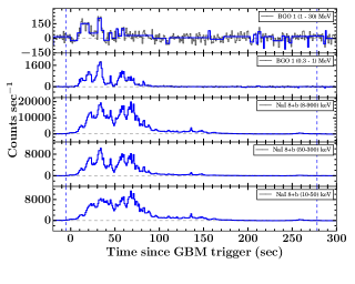
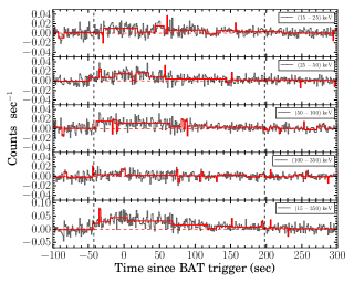
Figure 1: Prompt light curves$-$ Left panel: the Fermi GBM energy-resolved and background-subtracted light curves of GRB 171010A. The Bayesian blocks (blue) are overplotted to track the change in the light curve. The blue vertical dashed lines mark the time slice used for the GBM time-averaged spectral analysis. Right panel: the BAT energy-resolved mask-weighted light curves of GRB 171205A. The Bayesian block light curve for respective energy channels is shown in red colour. The black vertical dashed lines mark the time slice used for the BAT time-averaged spectral analysis.

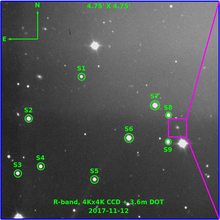
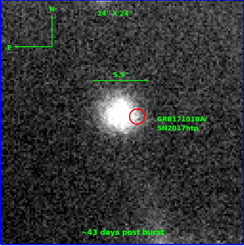
Figure 2: Left panel: a section of stacked $R$-band image (8$\times$300s; 4.75${}^{{}^{\prime}}$ $\times$ 4.75${}^{{}^{\prime}}$) of GRB 171010A/SN 2017htp field observed on 2017-11-22 using the 4K$\times$4K CCD Imager at the 3.6m DOT. Secondary standard stars (S1-–S9) are encircled; those were used for calibration. Right panel: a 24${}^{{}^{\prime\prime}}$ $\times$ 24${}^{{}^{\prime\prime}}$ section of the GRB field is shown to highlight the GRB 171010A/SN 2017htp embedded in the host galaxy.

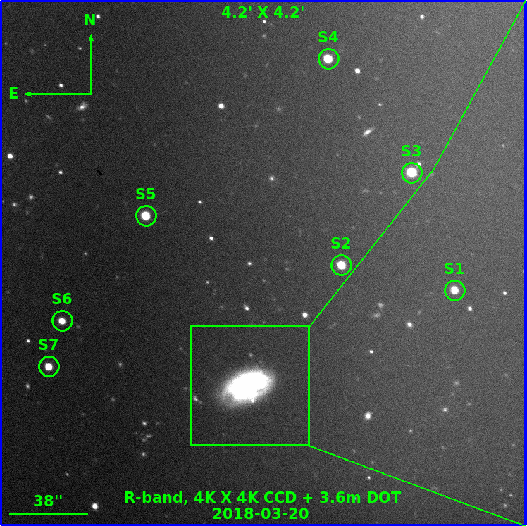
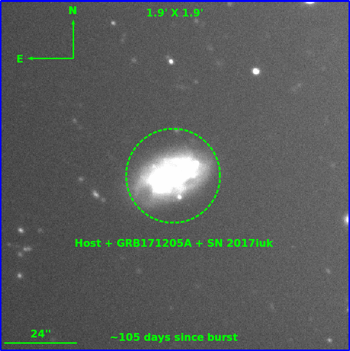
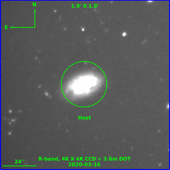
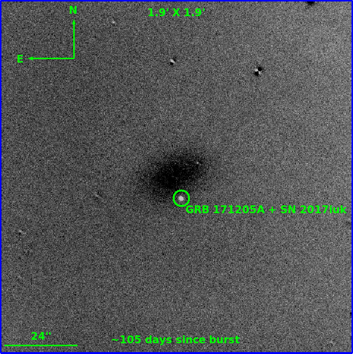
Figure 3: The finding chart of GRB 171205A/SN 2017iuk in the $R$-band is presented. The upper-left panel shows a 4.2${}^{{}^{\prime}}$ $\times$ 4.2${}^{{}^{\prime}}$ section of the image highlighting GRB171205A+SN 2017iuk+host and seven standard stars (S1–S7) used for calibration. The upper-right panel shows a 1.9${}^{{}^{\prime}}$ $\times$ 1.9${}^{{}^{\prime}}$ section of the image, zooming on GRB 171205A/SN 2017iuk associated with the host. The lower-left panel displays the $R$-band image of the field of GRB 171205A/SN 2017iuk observed on 2020-03-16 ($\sim$2.3 yrs post burst), used to perform the template subtraction. The lower-right panel presents the template subtracted image of GRB 171205A/SN 2017iuk, obtained by subtracting the frame of lower-left panel from the image shown in the upper-right panel.

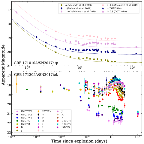
Figure 4: Upper panel: multi-band optical light curves of GRB 171010A/SN 2017htp. Data points plotted with star symbols are obtained based on the observations acquired using the 4K$\times$4K CCD Imager and 3.6m DOT, and those plotted with the filled colour-coded circles are taken from Melandri et al. (2019). The dotted lines present the contribution from the power-law decay of GRB 171010A afterglow and a constant flux from the host galaxy. Lower panel: multi-band light curves (UV–NIR) of GRB 171205A/SN 2017iuk plotted based on the data observed with the 4K$\times$4K CCD Imager/3.6m DOT (with colour-coded star symbols) along with those adopted from Izzo et al. (2019) (with circle symbols).

2.2 Optical observations and analysis

The late-time optical observations of the two events, i.e., GRB 171010A/SN 2017htp and GRB 171205A/SN 2017iuk were obtained using the 4K$\times$4K CCD Imager mounted at the 3.6m DOT (Pandey et al., 2018; Kumar et al., 2022), finding charts are shown in Figures 2 and 3, respectively. Observations of GRB/SNe cases presented in this study were acquired with 2$\times$2 binning, a gain of 5 e^-/ADU, and a readout speed of 1 MHz, having readout noise of $\sim$10 e^-.

2.2.1 GRB 171010A/SN 2017htp

The field of GRB 171010A/SN 2017htp was observed in the Bessel $R$-band on 2017-11-21 ($\sim$42d post burst) and detected the underlying GRB-SN embedded in a host galaxy. On 2017-11-22, we again observed the field of GRB 171010A/SN 2017htp in the Bessel $V$, $R$, and $I$ bands. The $R$-band image obtained on 2017-11-22 is shown in the left panel of Figure 2 with a field of view (FOV) of 4.75${}^{\prime}\times$4.75^′. However, to zoom in on the host embedded GRB 171205A/SN 2017iuk, a smaller section of the GRB field with a FOV of 24${}^{\prime\prime}\times$24^′′ is highlighted in the right panel of Figure 2. For the field calibration of GRB 171010A/SN 2017htp, Landolt photometric standard fields PG 1047 and SA98 (Landolt, 1992) were observed on 2021-12-11 along with the GRB field in the $UBVRI$ bands. The standard stars in the PG 1047 and SA98 fields have a $V$-band magnitude range of 11.88 to 15.67 mag and a B$-$V colour range of $-$0.29 to +1.41 mag. For consistency, the data reduction was performed using the procedure discussed in Melandri et al. (2019), and calibration was done using a standard procedure discussed in Kumar et al. (2021b) and utilising the python-scripts hosted on RedPipe (Singh, 2021). The nine secondary standard stars in the GRB field used for the calibration are encircled in the left panel of Figure 2 (S1–S9), whereas their calibrated magnitudes in $UBVRI$ bands are listed in Table LABEL:tab:171010A_secondary_stars. The complete log of observations of GRB 171010A/SN 2017htp, along with calibrated magnitudes, is tabulated in Table 1. The calibrated $V$, $R$, and $I$-band magnitudes of GRB 171010A/SN 2017htp are converted to the SDSS $r$ and $i$-band magnitudes using the transformation equations of Jordi et al. (2006). These $r$ and $i$-band magnitudes (with colour-coded star symbols) are plotted with those were reported by Melandri et al. (2019) in $g$, $r$, $i$, and $z$ bands (see the upper panel of Figure 4). The data have also been corrected for the Galactic extinction using E(B-V) = 0.13 mag (Schlafly & Finkbeiner, 2011); however, the host galaxy extinction was considered negligible (Melandri et al., 2019).

Table 1: Log of multi-band optical observations of GRB 171010A/SN 2017htp and GRB 171205A/SN 2017iuk obtained using the 4K$\times$4K CCD Imager mounted at the axial port of 3.6m DOT. Magnitudes are expressed in the AB system and not corrected for extinction.

JD	$\Delta$t (d)	Filter	Frame	Mag	Error
GRB 171010A/SN 2017htp
2458079.2916	41.999	R	2$\times$100s	20.24	0.06
			3$\times$300s
2458080.2342	42.942	I	6$\times$300s	19.43	0.10
2458080.1976	42.905	R	8$\times$300s	20.26	0.06
2458080.2570	42.965	V	6$\times$300s	20.79	0.09
GRB 171205A/SN 2017iuk
2458196.2464	103.440	I	3$\times$200s	21.13	0.06
2458196.2307	103.425	R	2$\times$300s	20.96	0.05
2458196.2384	103.432	B	3$\times$200s	21.56	0.10
2458198.2770	105.471	I	3$\times$200s	21.14	0.08
2458198.2680	105.462	R	3$\times$200s	20.05	0.03

For a typical GRB-SN event, three main flux components contribute at late epochs, i.e., 1) afterglow (AG) of the GRB, 2) the underlying SN, and 3) the constant flux from the host galaxy (see Cano et al. 2017 for a review). A great deal of physical information about such rare events can be obtained by modelling each of the three components individually. The host galaxy contribution can be extracted through the template-subtraction technique or by subtracting a constant flux of the host using very late time observations. The afterglow component can be separated by fitting either a single or a set of broken power laws to the early time observations. After removing both the host and afterglow contributions, the light curve of the underlying SN can be fetched. In the case of GRB 171010A/SN 2017htp, initially, light curves in all the optical bands followed a single-power law flux decay with $\alpha$ $\approx$ 1.42 $\pm$ 0.05 (Melandri et al., 2019); however, optical light curves started flattening from $\sim$3d post burst. Therefore to remove the contribution of the host galaxy and the afterglow of GRB 171010A, all the presented light curves in the upper panel of Figure 4 are fitted with a single power-law having $\alpha$ = 1.42 $\pm$ 0.05 plus a constant to account for the host galaxy contribution (shown with dashed lines) and to extract the light curve of the underlying SN 2017htp.

2.2.2 GRB 171205A/SN 2017iuk

The field of GRB 171205/SN 2017iuk was observed on 2018-03-18 and 2018-03-20 ($\sim$103 and 105d post burst) respectively in $BRI$ and $RI$ bands using the 4K$\times$4K CCD Imager at the 3.6m DOT. We again observed the field on 2020-03-16 (in $RI$ bands; $\sim$2.3 yrs post burst to perform image subtractions) and 2021-01-14 (in $UBVRI$ bands, $\sim$3.1 yrs post burst for image subtraction and calibrations). For the purpose of field calibrations, Landolt photometric standard field PG 1323 (Landolt, 1992) was also observed on 2021-01-14 along with the GRB field in the $UBVRI$ bands. The standard stars in PG 1323 have a $V$-band magnitude range of 12.09 to 14.00 mag and a B$-$V colour range of $-$0.14 to +0.76 mag. The $R$-band finding chart of GRB 171205A/SN 2017iuk and secondary standard stars (S1–S7) with a FOV of 4.2${}^{\prime}\times$4.2^′ are shown in the upper-left panel of Figure 3. A smaller section with a FOV of 1.9${}^{\prime}\times$1.9^′ of GRB 171205A/SN 2017iuk field is presented in the upper-right panel. The frame used for the template subtraction and the template subtracted image are shown respectively in the lower left and right panels of Figure 3. The template subtraction to remove the host galaxy contributions was performed with a standard procedure via matching FWHM and flux values of respective images using the python-based codes hosted on RedPipe (Singh, 2021). Calibrated $UBVRI$ magnitudes of seven secondary standard stars of the GRB/SN field are tabulated in Table LABEL:tab:secondary_stars_aa, whereas calibrated magnitudes of the GRB 171205A/SN 2017iuk thus obtained are tabulated in Table 1. These calibrated magnitudes are plotted (with star symbols) along with publicly available ones in $W2M2W1UBgVrRiIzJHK$ bands (with colour-coded circle legends) as reported by Izzo et al. 2019 (see the lower panel of Figure 4). The data have also been corrected for the host extinction of E(B-V) = 0.02 mag (Izzo et al., 2019) and a Galactic extinction of E(B-V) = 0.05 mag (Schlafly & Finkbeiner, 2011).

Since the beginning, optical afterglows of GRB 171205A have deviated from the power-law decay; however, light curves are completely dominated by the BB emission from SN 2017iuk after $\gtrsim$3d post-burst. Hence we considered the GRB 171205A afterglow contribution negligible at late times. The SN optical light-curve peak is observed around $\sim$11d post burst (de Ugarte Postigo et al., 2017; Izzo et al., 2019). In the case of GRB 171205A/SN 2017iuk, the host galaxy component is removed via performing template subtraction.

3 Results

This section describes major results emphasising the importance of prompt emission properties and underlying SNe properties of the two GRB-SNe in the optical and other similar objects.

3.1 High energy aspects

3.1.1 Prompt emission spectra

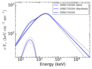
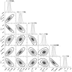
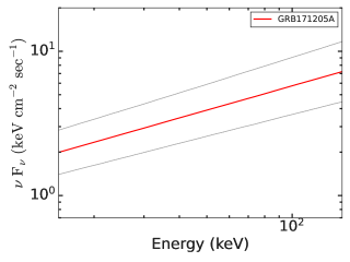
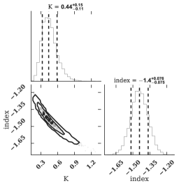
Figure 5: Time-averaged spectra$-$ Upper panel: the best fit Fermi GBM time-averaged (from T₀-5 to T₀ +278s) spectrum of GRB 171010A. Lower panel: the best fit Swift BAT time-averaged (from T₀-42.228 to T₀ +197.796s) spectrum of GRB 171205A. The corner plots obtained using 2000 number of simulations using Bayesian fitting are also shown for both bursts.

The Fermi GBM time-integrated spectrum of GRB 171010A (in model space, from T₀-5 to T₀ +278 s), along with the corner plot, is shown in the upper panel of Figure 5. It can be well explained using the Band plus Blackbody model. We obtained following spectral parameters for the best fit model: low-energy photon index ($\alpha$) = -1.06 $\pm$ 0.03, high-energy photon index ($\beta$) = 2.69 $\pm$ 0.09, peak energy ($E_{\rm p}$) = 211.69 $\pm$ 5.55 keV and temperature kT = 7.88 $\pm$ 0.28 keV. The $\alpha$ value is consistent with the prediction of synchrotron emission in slow and fast cooling cases. However, the detection of a thermal (photospheric) signature in combination with a non-thermal Band suggests a hybrid jet composition (a matter-dominated hot fireball and a colder magnetic-dominated Poynting flux component) for GRB 171010A. We compared the observed energy fluence of GRB 171010A with all GBM detected GRBs (see Figure 6) and proposed that GRB 171010A is the third most GBM fluent burst.

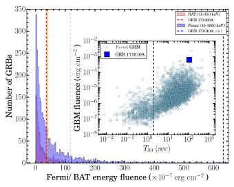
Figure 6: Observed fluence distribution$-$ The fluence distributions for GBM (blue) and BAT (red) detected GRBs in the 10-1000 and 15-150 keV energy ranges, respectively. The vertical solid dark orange and dashed sky blue lines show the mean values of the BAT and GBM samples, respectively. The positions of GRB 171010A and GRB 171205A are shown with blue and red dashed vertical lines, respectively. The inset diagram presents the energy fluence as a function of $T_{\rm 90}$ distribution of GBM detected bursts. The position of GRB 171010A is shown with a blue square. The vertical black dashed line corresponds to the $T_{\rm 90}$ = 2s.

We also performed the Swift BAT time-averaged (from T₀-42.228 to T₀ +197.796 s) spectral analysis of GRB 171205A using the 3ML tool and Bayesian fitting. We noticed that the Swift BAT time-averaged spectrum of GRB 171205A is best fitted by the power-law model (lowest BIC value) with a photon index of 1.44 $\pm$ 0.08. The best fit spectrum, along with the corner plot, is shown in the lower panel of Figure 5. During the time-integrated temporal window, we estimated the fluence equal to $\approx$(3.6 $\pm$ 1.6) $\rm\times 10^{-6}erg~{}cm^{-2}$ in 15-150 keV energy range. Once compared with the distribution of the BAT fluence in 15-150 keV for all the Swift BAT detected bursts, we find that the energy fluence of GRB 171205A is close to the mean value $\approx$(3.8 $\rm\times 10^{-6}erg~{}cm^{-2}$) of the sample (see Figure 6).

3.1.2 Prompt emission characteristics

Spectral peak-duration distribution:

The lGRBs are believed to have a softer spectrum in comparison to those observed for the majority of sGRBs (Kouveliotou et al., 1993b). We determined the time-integrated spectral $E_{\rm p}$ (hardness) of GRB 171010A and GRB 171205A and placed them in $E_{\rm p}$-$T_{\rm 90}$ plane to compare with a larger sample of bursts detected by the Fermi GBM (see the left panel of Figure 7). We found that both GRBs have softer $E_{\rm p}$ values and durations longer than 100s. GRB 171010A and GRB 171205A lie towards the right edge in the spectral peak-duration distribution plane and follow the typical characteristics of lGRBs.

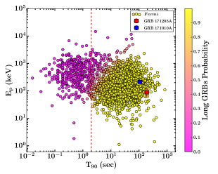
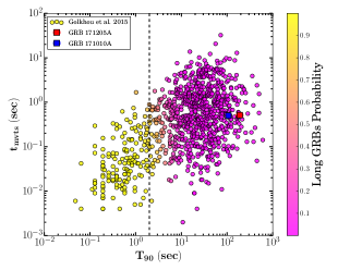
Figure 7: Spectral hardness$-$ Left panel: $E_{\rm p}$-$T_{\rm 90}$ diagram. A sample of long and short GRBs taken from the Fermi GBM catalogue is shown. The positions of GRB 171010A and GRB 171205A are highlighted with blue and red squares, respectively. The right side Y-scale represents the probability of lGRBs. The vertical red dashed line shows the line of the traditional classification of GRBs. Right panel: $t_{\rm mvts}$-$T_{\rm 90}$ diagram. The $t_{\rm mvts}$ versus $T_{\rm 90}$ for GRB 171010A (blue square) and GRB 171205A (red square) are plotted with a sample of long and short GRBs adopted from Golkhou et al. (2015) are presented. The vertical black dashed line guides the eyes to look at the traditional classification of GRBs.

Minimum Variability Time scale:

We determined the minimum variability time scales ($t_{\rm mvts}$) of GRB 171010A and GRB 171205A using the Bayesian block algorithm on count rate prompt emission light curve in GBM 8-900 keV and BAT 15-350 keV, respectively (see Figure 1). The Bayesian blocks follow the statistically significant changes in the count rate light curves of GRB 171010A and GRB 171205A. We calculated the minimum bin size of the Bayesian blocks. The half of the minimum bin size of Bayesian blocks is considered as $t_{\rm mvts}$ (Vianello et al., 2018). The right panel of Figure 7 shows the $t_{\rm mvts}$-$T_{\rm 90}$ distribution for a sample of long and short GRBs studied by Golkhou et al. (2015). We found that the $t_{\rm mvts}$ values of both the bursts are nearly comparable. The positions of GRB 171010A and GRB 171205A are shown with blue and red squares, respectively, and they lie towards the right edge of the distribution. We also calculated the probability of lGRBs of the sample studied by Golkhou et al. (2015) using the Gaussian mixture model.

3.1.3 Prompt Correlation$-$Amati

We examine the correlation between the rest-frame $E_{\rm p}$ and isotropic equivalent gamma-ray energy ($E_{\rm\gamma,iso}$) for GRB 171010A and GRB 171205A in the Amati plane (Amati, 2006). In the case of GRB 171010A, we calculated the $E_{\rm p}$ and $E_{\rm\gamma,iso}$ of the burst from the time-integrated spectral modelling of GBM data. As the Swift BAT instrument has a limited spectral coverage (15-150 keV), therefore, in the case of GRB 171205A, we calculated the time-integrated $E_{\rm p}$ using the correlation between the observed BAT fluence and $E_{\rm p}$ (Zhang et al., 2020), i.e., $E_{\rm p}$ = [fluence/($\rm 10^{-5}erg~{}cm^{-2}$)]^0.28 $\rm\times 117.5^{+44.7}_{-32.4}$ keV $\approx$ 88.27${}^{+33.58}_{-24.34}$ keV, a softer value of $E_{\rm p}$, typically observed for lGRBs. The calculated $E_{\rm p}$ value of GRB 171205A is consistent with that reported by D’Elia et al. (2018) using joint Konus-Wind and BAT observations. To estimate the $E_{\rm\gamma,iso}$ for GRB 171205A, we used equation 6 of Fong et al. (2015).

The calculated $E_{\rm\gamma,iso}$ values suggest that GRB 171010A is a luminous burst (Chand et al., 2019); however, GRB 171205A is a llGRB. Amati correlation for GRB 171010A and GRB 171205A along with a sample of lGRBs taken from Minaev & Pozanenko (2020) and a set of llGRBs adopted from Chand et al. (2020) is shown in Figure 8. We noticed that despite being connected to SNe, GRB 171205A is an outlier to the Amati correlation (D’Elia et al., 2018), similar to other llGRBs; on the other hand, GRB 171010A is well consistent with this correlation. Generally, llGRBs are not agreeable with the Amati correlation as the radiation from these sources is powered by shock breakout (Nakar & Sari, 2012; Barniol Duran et al., 2015; Chand et al., 2020) among other alternate reasons. For llGRBs, the energetics satisfy a fundamental correlation which is helpful in constraining the observed duration of the burst (Nakar & Sari, 2012). We have used equation 18 of Nakar & Sari (2012) to estimate the observational duration for GRB 171205A due to shock breakout and found $\sim$ 300 s, which is in agreement with the observed $T_{\rm 90}$ duration of the burst within errors. This indicates that GRB 171205A might be originated due to shock breakout, as seen for a few other llGRBs (Nakar & Sari, 2012; Chand et al., 2020). Alternatively, D’Elia et al. (2018) discussed that GRB 171205A lies outside the Amati correlation based on joint Swift and Konus-Wind observations and using a different spectral analysis method. They also mentioned that GRBs observed off-axis could not be consistent with the Amati correlation, whereas GRBs with on-axis observations generally follow this correlation. In the case of GRB 171205A, the source was observed off-axis; it might also be a possible cause for the burst to be an outlier in the Amati correlation. Further, Martone et al. (2017) suggested that if an old generation instrument observes a particular GRB (i.e., GRB 980425 and GRB 031203), that might cause a false outlier of Amati correlation, although this possibility is less likely for GRB 171205A as Swift (new generation instrument) and Konus-Wind both confirmed that the burst is an Amati outlier. In the light of the above, we suggest that GRB 171205A could not be an outlier to the Amati correlation due to the observational biases rather than the intrinsic nature of typical llGRBs (shock breakout or off-axis view).

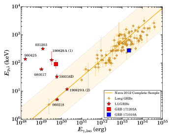
Figure 8: Amati correlation: GRB 171010A (blue square) and GRB 171205A (red square) in Amati correlation along with the samples of lGRBs (taken from; Minaev & Pozanenko, 2020) and llGRBs (adopted from; Chand et al., 2020). The figure clearly indicates that GRB 171010A is well consistent with the Amati correlation, whereas GRB 171205A is an outlier to this correlation, as seen in the case of other well-studied llGRBs.

3.1.4 Possible central engines

A central engine powering source is widely accepted to explain the formation of lGRBs. It could be in the form of a mass accreting black hole (Woosley, 1993; MacFadyen & Woosley, 1999) or a millisecond magnetar (Duncan & Thompson, 1992; Usov, 1992; Thompson & Duncan, 1993). To constrain the possible central engines of GRB 171010A and GRB 171205A, we used methods presented in Sharma et al. (2021). The key idea of this method is based on the maximum possible rotational energy of the order of $\sim$10⁵² erg to launch jets from a millisecond magnetar. For this purpose, we determined the jet opening angles and beaming-corrected gamma-ray energy ($E_{\rm\gamma,beamed}$) for both the bursts. We constrained lower limits on the jet opening angle using equation 4 given in Frail et al. (2001). We assumed typical values of number density of medium ($n_{0}$ = 1) and thermal energy fraction in electrons ($\epsilon_{e}$ = 0.1) to calculate the jet opening angles (Panaitescu & Kumar, 2002; Gupta et al., 2021a).

In the case of GRB 171010A, we considered second temporal break as jet break time (see Section 3.2) and found $\theta_{j}$ = 5.43^∘ translated to $E_{\rm\gamma,beamed}$ equal to 9.91 $\times~{}10^{50}$ erg. On the other hand, in the case of GRB 171205A, we used the last XRT data points to constrain the limits on the jet opening angle. We found a very wide opening angle $\theta_{j}$ $>$ 51.3^∘ and $E_{\rm\gamma,beamed}$ $>$ 1.99 $\times~{}10^{49}$ erg. We noticed that for both the cases, $E_{\rm\gamma,beamed}$ values are less than the maximum possible rotational energy budget of a typical magnetar (Haensel et al., 2009). Therefore, this method indicates that the magnetars could be the central engine for the two bursts under discussion. The existence of a Kerr Black Hole as an inner engine demands a higher energy budget among other observed properties (van Putten & Della Valle, 2017; Sharma et al., 2021). The left panel of Figure 9 shows the number distribution of $E_{\rm\gamma,beamed}$ of all the GBM detected bursts taken from Sharma et al. (2021). The locations of GRB 171010A and GRB 171205A are also marked using blue and red lines, respectively.

We further utilised the method discussed by Li et al. (2018) to constrain the possible central engine of GRB 171205A investigating an $X$-ray plateau followed by a normal decay phase. Li et al. (2018) performed the analysis of the $X$-ray afterglow light curve having plateau phases of 101 bursts (up to May 2017). They measured redshift values by calculating the isotropic $X$-ray ($E_{\rm X,iso}$) and kinetic ($E_{\rm K,iso}$) energies and compared them with the maximum energy budget of magnetars. In the case of GRB 171205A, we calculated the $E_{\rm X,iso}$ (2.59 $\times~{}10^{47}$ erg) using equation 7 of Li et al. (2018). Further, we followed the methodology discussed by Li et al. (2018) to calculate the $E_{\rm K,iso}$ and have applied the closure relations during the normal decay phase of GRB 171205A to constrain the spectral regime. We found that the normal decay phase could be explained if the observed frequencies $\rm\nu_{X}>max(\nu_{c},\nu_{m})$; where $\nu_{c},\nu_{m}$ are the cooling and maximum synchrotron break frequencies for the external forward shock model both for ISM and wind like ambient media. We used equation 9 of Li et al. (2018) to calculate $E_{\rm K,iso}$ (1.01 $\times~{}10^{51}$ erg) for GRB 171205A; for micro-physical parameters: $\epsilon_{e}$ = 0.1, thermal energy fraction in magnetic filed ($\epsilon_{B}$) = 0.01, $n_{0}$ = 1, and the Compton parameter (Y) = 1. The distribution of $E_{\rm X,iso}$ and $E_{\rm K,iso}$ for the defined gold, silver, and bronze samples taken from Li et al. (2018) are shown in the right panel of Figure 9. GRB 171205A lies towards the lower-left edge of the distribution, and its position is marked with a red square. The measured values of $E_{\rm X,iso}$ and $E_{\rm K,iso}$ for GRB 171205A are less than the maximum energy budget of magnetars and belong to the bronze sample of Li et al. (2018), providing a clue that magnetar could be the possible central engine for GRB 171205A. However, we could not implement this method for GRB 171010A due to the non-existence of the plateau phase followed by a normal decay phase in the XRT light curve.

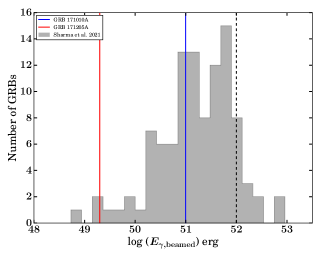
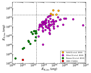
Figure 9: Possible central engine$-$ Left panel: distribution of $E_{\rm\gamma,beamed}$ for all GRBs detected by GBM, taken from Sharma et al. (2021). The blue and red lines highlight the respective positions of GRB 171010A and GRB 171205A. The vertical black line shows the maximum possible rotational energy of the magnetar. Right panel: the distribution of $E_{\rm X,iso}$ and $E_{\rm K,iso}$ for gold (orange), silver (magenta), and bronze (green) samples of Li et al. (2018) is shown. The position of GRB 171205A is marked with a red square. The vertical and horizontal black dashed lines show the maximum possible energy budget of a magnetar as a central engine powering source.

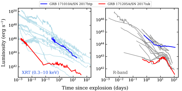
Figure 10: $X$-ray and $R$-band afterglow light curves$-$ the XRT and optical $R$-band light curves of GRB 171010A/SN 2017htp (shown with blue) and GRB 171205A/SN 2017iuk (shown with red) along with the XRT-observed light curves of all known GRB/SNe cases are shown in the left and right panels, respectively. GRB 171010A/SN 2017htp and GRB 171205A/SN 2017iuk respectively appear among the brightest and faintest GRB/SNe.

3.2 $X$-ray and optical light curves comparison

In this section, $X$-ray and optical $R$-band light curves of GRB 171010A/SN 2017htp and GRB 171205A/SN 2017iuk are compared with those of 13 other well studied XRT-detected GRB/SNe cases (see the left and right panels of Figure 10, respectively). The comparison sample includes : GRB 050525A/SN 2005nc (@$z$ = 0.606), GRB 081007A/SN 2008hw (@$z$ = 0.530), GRB 091127A/SN 2009nz (@$z$ = 0.490), GRB 101219B/SN 2010ma (@$z$ = 0.552), GRB 111209A/SN 2011kl (@$z$ = 0.677), GRB 130702A/SN 2013dx (@$z$ = 0.145), GRB 130831A/SN 2013fu (@$z$ = 0.479; Cano et al., 2017, and references therein), GRB 060218/SN 2006aj (@$z$ = 0.033; Ferrero et al., 2006), GRB 120422A/SN 2012bz (@$z$ = 0.282; Schulze et al., 2014), GRB 130427A/SN (@$z$ = 0.340; Perley et al., 2014), GRB 190114C/SN (@$z$ = 0.425; Misra et al., 2021; Gupta et al., 2022), GRB 190829A/SN 2019oyw (@$z$ = 0.078; Hu et al., 2021), GRB 200826A/SN (@$z$ = 0.748; Ahumada et al., 2021; Rossi et al., 2022). For the events with observations only in the SDSS filters, the $i$-band data is adopted in place of the $R$-band. The light curves plotted in Figure 10 are also corrected for the cosmological expansion.

The catalogue XRT results for GRB 171010A suggests that the count rate XRT light curve could be best fitted using power-law model with two breaks with following temporal parameters: $\alpha_{1,2,3}$= 2.17${}^{+0.29}_{-0.33}$, 0.28${}^{+0.91}_{-1.78}$, 1.83${}^{+0.16}_{-0.14}$ and T_b1,b2= 7${}^{+4}_{-3}$ $\times~{}10^{4}$s, 1.7${}^{+0.9}_{-0.3}$ $\times~{}10^{5}$s . We considered that the second break is due to jet break (although achromatic behaviour could not be confirmed due to the unavailability of simultaneous multiwavelength data) as the temporal index post-break is consistent with the expected temporal index during jet phase (Chand et al., 2019). On the other hand, the XRT count rate light curve of GRB 171205A could be best fitted using power-law model with three breaks with following temporal parameters: $\alpha_{1,2,3,4}$= 1.26${}^{+0.39}_{-0.27}$, 2.30${}^{+0.05}_{-0.05}$, 0.02${}^{+0.08}_{-0.10}$, 0.98${}^{+0.08}_{-0.07}$ and T_b1,b2,b3= 196${}^{+38}_{-9}$s, 5848${}^{+641}_{-267}$s, 9.6${}^{+1.8}_{-1.4}$ $\times~{}10^{4}$s, clearly showing a plateau in the XRT light curve. We noticed that the $X$-ray and $R$-band light curves of nearby GRB 171205A/SN 2017iuk are one of the faintest in the present sample of a total of 15 GRB/SNe, typically expected in case of llGRBs or bursts observed off-axis (D’Elia et al., 2018). On the other hand, at both wavebands, GRB 171010A/SN 2017htp appeared as one of the brightest GRB/SNe cases, possibly observed on-axis at moderate distances (Chand et al., 2019).

3.3 Optical light curves modelling

In this section, we describe methods used to generate the bolometric light curves of SN 2017htp and SN 2017iuk and their semi-analytical modelling using the MINIM code (Chatzopoulos et al., 2013).

3.3.1 Bolometric light curves

The pseudo-bolometric light-curves of SN 2017htp ($griz$) and SN 2017iuk ($UgBrViRIzJHK$) are produced using the python-based Superbol code (Nicholl, 2018), as discussed in Kumar et al. (2020a, 2021b); Pandey et al. (2021). To compute the multi-band fluxes at similar epochs, interpolations/extrapolations were done wherever necessary by assuming constant colours. Possible contributions of $UV$ and $NIR$ fluxes are included by extrapolating the SED and integrating the observed fluxes to obtain the full bolometric light curves for both events. The full bolometric light-curve ($UV$ to $NIR$; $L_{bol}$) of SN 2017htp is obtained from $\sim$7 to 35 rest-frame days post burst, which exhibits a peak bolometric luminosity ($L_{peak}$) of $\sim$(2.1 $\pm$ 0.9) $\times$ 10⁴³ erg s^-1 (in faded red color; see Figure 11). Although, higher error bars are associated with the bolometric light curve of SN 2017htp due to inadequate observed frequency coverage, giving rise to significant uncertainty in the SED fitting. On the other hand, bolometric light-curve of SN 2017iuk (from $\sim$3 to 102 rest-frame days post burst) shows a comparatively lower $L_{peak}$ of $\sim$(0.52 $\pm$ 0.06) $\times$ 10⁴³ erg s^-1 (plotted with the green color in Figure 11).

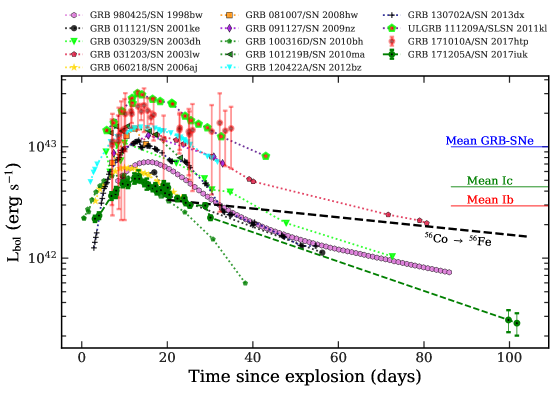
Figure 11: The bolometric light curves of SN 2017htp and SN 2017iuk generated using the Superbol code (Nicholl, 2018) are compared with those of other well-studied GRB-SNe taken from (Cano et al., 2017, and references therein). The mean $L_{peak}$ of Type Ib, Ic (Lyman et al., 2016), and GRB-SNe (excluding SLSN 2011kl; Cano et al. 2017) along with the ⁵⁶Co $\rightarrow$ ⁵⁶Fe theoretical decay curve have also been marked for the comparison. SN 2017htp appears to be one of the brightest, and SN 2017iuk is among the faintest GRB-SNe. GRB-SNe presented here exhibit more than an order of magnitude range in bolometric luminosity units.

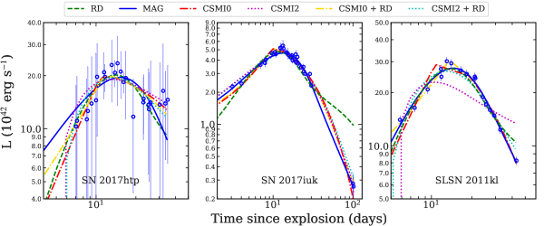
Figure 12: Semi-analytical light-curve modelling of SN 2017htp, SN 2017iuk, and SLSN 2011kl is performed using the MINIM code (Chatzopoulos et al., 2013) and shown in the left, middle, and right panels, respectively. For all three above-mentioned GRB-SNe, $\kappa$ = 0.07 cm² g^-1 is adopted.

The bolometric light curves of SN 2017htp and SN 2017iuk are compared with those of other well-studied GRB-SNe taken from Cano et al. (2017) (see Figure 4). The mean $L_{peak}$ of Type Ib, Ic (Lyman et al., 2016), and GRB-SNe (excluding SLSN 2011kl; Cano et al., 2017) are also marked for comparison. SN 2017htp shares one of the brightest $L_{peak}$ than those of other GRB-SNe presented in this study (except SLSN 2011kl; $L_{peak}$ $\sim$[2.9 $\pm$ 0.1] $\times$ 10⁴³ erg s^-1) and also higher than mean $L_{peak}$ quoted for GRB-SNe. On the other hand, SN 2017iuk is one of the low-luminosity GRB-SNe and exhibits a fainter $L_{peak}$ in comparison to those of SN 2017htp, SLSN 2011kl, other plotted GRB-SNe, and mean $L_{peak}$ marked for GRB-SNe, whereas comparable with the mean $L_{peak}$ of SNe Ic. SLSN 2011kl is the only SLSN associated with a ulGRB and shows the brightest $L_{peak}$ among all GRB-SNe (see Figure 11); however, it is the faintest to date in comparison to all other SLSNe I (Kann et al., 2019).

Table 2: Best-fitting parameters for the RD, MAG, CSMI0, CSMI2, CSMI0+RD, and CSMI2+RD models that fitted to the bolometric light curves of SN 2017htp, SN 2017iuk, and SLSN 2011kl using the MINIM code (Chatzopoulos et al., 2013). Based on the physical reliability of the estimated parameters, the bolometric light curve of SN 2017htp can be explained using the RD/MAG/CSM models, SLSN 2011kl by the MAG/CSM models, and the light curve of SN 2017iuk can be explained only using the MAG model.

				RD model
SN	$A_{\gamma}^{a}$	$M_{\rm Ni}^{b}$	$t_{d}^{c}$	$M_{\rm ej}$					$\chi^{2}$/DOF
	(109)	($M_{\odot}$)	(d)	($M_{\odot}$)
SN2017htp	7.25 $\pm$ 2.88	0.76 $\pm$ 0.07	18.72 $\pm$ 1.64	3.27 $\pm$ 0.57					0.11
SN2017iuk	3.66 $\pm$ 2.40	0.18 $\pm$ 0.01	10.76 $\pm$ 0.62	2.31 $\pm$ 0.27					11.13
SLSN2011kl	3.51 $\pm$ 2.44	1.04 $\pm$ 0.01	10.81 $\pm$ 0.16	1.56 $\pm$ 0.05					3.76
				MAG model
SN	$R_{0}^{d}$	$E_{p}^{e}$	$t_{d}$	$t_{p}^{f}$	$v_{\rm exp}$	$P_{i}$	$B$	$M_{\rm ej}$	$\chi^{2}$/DOF
	($10^{13}$ cm)	($10^{51}$ erg)	(d)	(d)	($10^{3}$ km s-1)	(ms)	($10^{14}$ G)	($M_{\odot}$)
SN2017htp	0.03 $\pm$ 0.03	0.12 $\pm$ 0.01	17.05 $\pm$ 0.82	10.41 $\pm$ 0.92	14.47 $\pm$ 0.98	12.89 $\pm$ 0.04	8.72 $\pm$ 0.26	2.80 $\pm$ 0.27	0.17
SN2017iuk	0.04 $\pm$ 0.02	0.03 $\pm$ 0.0001	17.06 $\pm$ 0.10	9.85 $\pm$ 0.46	29.02 $\pm$ 3.51	26.42 $\pm$ 0.01	18.36 $\pm$ 0.30	5.62 $\pm$ 0.07	1.04
SLSN2011kl	0.03 $\pm$ 0.02	0.14 $\pm$ 0.001	12.70 $\pm$ 0.29	16.08 $\pm$ 0.74	29.65 $\pm$ 5.34	11.93 $\pm$ 0.01	6.49 $\pm$ 0.08	3.18 $\pm$ 0.14	1.21
				CSMI0 model
SN	$R_{p}^{g}$	$M_{\rm ej}$	$M_{\rm csm}^{h}$	$\dot{M}$	$M_{Ni}$	$v_{\rm exp}$			$\chi^{2}$/DOF
	($10^{13}$ cm)	($M_{\odot}$)	($M_{\odot}$)	(10-2 $\times$ $M_{\odot}$ yr-1)	($M_{\odot}$)	($10^{3}$ km s-1)
SN2017htp	0.08 $\pm$ 0.01	5.31 $\pm$ 1.02	2.62 $\pm$ 1.24	0.0018 $\pm$ 0.0016	0.0 $\pm$ 0.0	14.15 $\pm$ 1.26			0.08
SN2017iuk	0.09 $\pm$ 0.01	2.40 $\pm$ 0.11	1.23 $\pm$ 0.02	0.0019 $\pm$ 0.0001	0.0 $\pm$ 0.0	8.42 $\pm$ 0.05			1.16
SLSN2011kl	0.11 $\pm$ 0.02	5.61 $\pm$ 0.17	1.35 $\pm$ 0.11	0.001 $\pm$ 0.00003	0.0 $\pm$ 0.0	15.27 $\pm$ 0.09			2.85
				CSMI2 model
SN2017htp	0.07 $\pm$ 0.03	6.46 $\pm$ 1.62	4.37 $\pm$ 2.37	4.16 $\pm$ 1.08	0.0 $\pm$ 0.0	14.16 $\pm$ 0.50			0.13
SN2017iuk	1.47 $\pm$ 1.38	20.39 $\pm$ 0.87	0.98 $\pm$ 0.02	19.98 $\pm$ 0.04	0.0 $\pm$ 0.0	6.55 $\pm$ 0.02			0.79
SLSN2011kl	1.32 $\pm$ 1.26	19.88 $\pm$ 0.09	1 $\pm$ 0.01	20 $\pm$ 0.04	0.0 $\pm$ 0.0	6.53 $\pm$ 0.02			0.87
				CSMI0+RD model
SN2017htp	0.09 $\pm$ 0.02	4.53 $\pm$ 1.21	2.37 $\pm$ 0.83	0.0012 $\pm$ 0.0015	0.14 $\pm$ 0.18	13.28 $\pm$ 1.34			0.08
SN2017iuk	0.09 $\pm$ 0.01	2.53 $\pm$ 0.14	1.03 $\pm$ 0.02	0.0013 $\pm$ 0.0001	0.02 $\pm$ 0.002	8.20 $\pm$ 0.07			0.96
SLSN2011kl	0.08 $\pm$ 0.01	3.39 $\pm$ 0.15	1.26 $\pm$ 0.07	0.00017 $\pm$ 0.00004	0.37 $\pm$ 0.03	14.45 $\pm$ 0.07			0.52
				CSMI2+RD model
SN2017htp	7.52 $\pm$ 7.47	2.69 $\pm$ 2.39	10.75 $\pm$ 4.99	3.64 $\pm$ 0.65	0.26 $\pm$ 0.08	12.67 $\pm$ 1.35			0.10
SN2017iuk	0.04 $\pm$ 0.01	19.6 $\pm$ 5.97	1.00 $\pm$ 0.01	0.20 $\pm$ 0.01	0.006 $\pm$ 0.01	5.08 $\pm$ 0.14			0.95
SLSN2011kl	0.03 $\pm$ 0.01	7.53 $\pm$ 0.36	21.57 $\pm$ 4.23	1.14 $\pm$ 0.08	0.72 $\pm$ 0.01	5.11 $\pm$ 0.05			3.85

• $A_{\gamma}$: optical depth for the gamma-rays measured after 10d post burst.

• $M_{\rm Ni}$: radioactive ⁵⁶Ni synthesized mass.

• $t_{d}$: effective diffusion timescale.

• $R_{0}$: progenitor radius.

• $E_{p}$: rotational energy.

• $t_{p}$: spin-down timescale of the magnetar.

• $R_{p}$: progenitor radius before the explosion.

• $M_{\rm csm}$: CSM mass.

Table 3: Best fit models and estimated crucial parameters that explain the bolometric light curves of SN 2017htp, SN 2017iuk, and SLSN 2011kl are summarised.

SN	Type	$M_{ej}$	$v_{exp}$	$P_{i}$	$B$	$R_{0}$	Best-fit
		($M_{\odot}$)	($10^{3}$ km s-1)	(ms)	($10^{14}$ G)	($10^{13}$ cm)	model
SN 2017htp	Ic BL	2.5-6.3	13.5-15.4	12.9 $\pm$ 0.1	8.7 $\pm$ 0.3	0.01–0.11	RD/MAG/CSM
SN 2017iuk	Ic BL	5.6 $\pm$ 0.1	29.0 $\pm$ 3.5	26.4 $\pm$ 0.1	18.4 $\pm$ 0.3	0.04 $\pm$ 0.02	MAG
SLSN 2011kl	SLSN I	3-5.8	14.4-35	11.9 $\pm$ 0.1	6.5 $\pm$ 0.1	0.01–0.13	MAG/CSM

3.3.2 Semi-analytical light-curve modelling

As a part of the present work, the bolometric light curves of SN 2017htp and SN 2017iuk are used to fit with six semi-analytical models utilising the MINIM code: radioactive decay of ⁵⁶Ni (RD), spin-down millisecond magnetar (MAG), constant density circumstellar interaction (CSMI0), wind-like CSMI (CSMI2), and HYBRID models (CSMI0+RD and CSMI2+RD; Chatzopoulos et al., 2013); see Figure 12. MINIM is a $\chi^{2}$-minimization code implemented in C++ and uses the random search technique to find the global minim. Details about the MINIM code and the models used here are well described in Chatzopoulos et al. (2012, 2013). In terms of light-curve modelling, previous studies attempted to regenerate the light curves of SN 2017htp (Melandri et al., 2019) and SN 2017iuk (Izzo et al., 2019) only using the RD model. Light-curve modelling of SLSN 2011kl is also discussed in the present analysis; because it is the only known SLSN stretching the limits of brightness and types of SNe connected to GRBs. For all the MINIM models discussed above, we adopted the electron-scattering opacity ($\kappa$) = 0.07 cm² g^-1, as also suggested by Izzo et al. (2019); Melandri et al. (2019). In the case of RD and MAG models, the M_ej values are calculated using equation 10 of Chatzopoulos et al. (2012). In MAG model, initial spin period of magnetar in ms is estimated using $P_{i}=(2\times 10^{50}$erg s^-1 /$E_{p})^{0.5}\times 10$ and magnetic field is calculated in gauss as $B=(1.3P_{10}^{2}/t_{p,yr})^{0.5}\times 10^{14}$; here $t_{p,yr}$ stands for the spin-down timescale of the magnetar in years (Chatzopoulos et al., 2013).

In the present analysis, at the same time, multiple models reproduced the bolometric light curves of all GRB-SNe with $\chi^{2}$/DOF $<$1 (see Table 2). The possible reasons behind $\chi^{2}$/DOF $<$ 1 are the association of higher error bars to the data points, a lower number of data points, and the larger number of fitting parameters. Hence, in the current analysis, $\chi^{2}$/DOF is not used as a benchmark to select the most suitable model but is only used to choose the model parameters that adequately regenerate the light curve. At the same time, we focused more on the level of the physical significance of the parameters estimated by different models, as also suggested by Kumar et al. (2021b); Pandey et al. (2021).

Statistically, the bolometric light curve of SN 2017htp is well-reproduced by all the six models (RD, MAG, CSMI0, CSMI2, CSM0+RD, and CSM2+RD) with $\chi^{2}$/DOF $<$ 1 (see the left panel of Figure 12). Hence as discussed above, to choose the most reliable model, we concentrated on the physical reliability of the estimated parameters. In the case of CSMI2 and CSMI2+RD models, the values of progenitor mass-loss rates ($\dot{M}$) are unphysically higher; therefore, these can not be considered as most suitable models for SN 2017htp. On the other hand, the parameters estimated by the other four models (RD, MAG, CSMI0, CSMI0+RD) are physically viable. So, RD, MAG, and CSMI models are equally favourable in explaining the light curve of SN 2017htp and based on the light curve modelling results only; it is not possible to discriminate any of these models. However, along with the light curve modelling results, the prompt analysis also supports a magnetar as a central engine powering source for SN 2017htp (see Section 3.1.4). All the parameters derived using the MINIM modelling of SN 2017htp are listed in Table 2.

In the case of SN 2017iuk, the RD model is unable to reproduce the late time observations (at $\sim$100d) and exhibits a poorer fit with $\chi^{2}$/DOF = 11.13. On the other hand, the rest five models reproduced the bolometric light curve of SN 2017iuk with $\chi^{2}$/DOF $\approx$1 (see the middle panel of Figure 12). However, CSMI0, CSMI2, CSMI0+RD, and CSMI2+RD models gave unphysical values of expansion velocities $v_{exp}$ $<$8,500 km s^-1, very low for a type Ic-BL SN and also much lower than the value estimated by Wang et al. (2018); Izzo et al. (2019) based on the spectral analysis. In addition, the values of $\dot{M}$ constrained by the CSMI2 and CSMI2+RD models are also unphysically higher. So, RD, CSMI, and RD+CSMI can not be considered probable powering mechanisms for SN 2017iuk. On the other hand, the bolometric light curve of SN 2017iuk is well-reproduced by the MAG model with physically viable parameters. So, the MAG model seems like the most suitable one for SN 2017iuk, which is also in agreement with the results discussed in Section 3.1.4. All the fitted parameters for the SN 2017iuk using the MINIM code are tabulated in Table 2.

In the case of SLSN 2011kl light curve modelling (see the right panel of Figure 12), the $M_{ej}$ value derived using the RD model is very low in comparison to those generally observed for SLSNe I (Nicholl et al., 2015). At the same time, CSMI2 and CSMI2+RD models suggested comparatively lower values of $v_{exp}$ and higher values of $\dot{M}$ in comparison to what is generally seen for GRB-SNe (Woosley & Bloom, 2006; Woosley & Heger, 2006; Smith, 2014). On the other hand, MAG, CSMI0, and CSMI0+RD models reproduced the bolometric light curve of SLSN 2011kl with physically reliable parameters and $\chi^{2}$/DOF close to one. The complete list of estimated parameters using the above models for SLSN 2011kl is tabulated in Table 2. So, based on the present analysis, CSMI and spin down millisecond magnetar are the possible powering sources of SLSN 2011kl.

In all, results from the light-curve modelling using the MINIM code clearly indicate that the model considering a spin down millisecond magnetar as a central engine powering source is the only model which can explain the light curves of all three GRB-SNe discussed presently. In addition, the light-curve model fittings help to constrain various crucial parameters of SN 2017htp, SN 2017iuk, and SLSN 2011kl that are tabulated in Table 3.

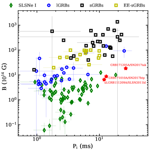
Figure 13: Modelled values of $B$ versus $P_{i}$ as constrained for SN 2017htp, SN 2017iuk, and SLSN 2011kl are compared with those of well studied sGRBs (Suvorov & Kokkotas, 2021), EE-sGRBs (Gibson et al., 2017), lGRBs (Li et al., 2018), and SLSNe I (Kumar et al., 2021b, and references therein).

3.4 Magnetars and $B$ versus $Pi$

Magnetars are expected to be the central powering sources for many energetic transients, including a certain class of GRBs and SNe (Duncan & Thompson, 1992; Usov, 1992; Wheeler et al., 2000; Metzger et al., 2015; Lin et al., 2020). Magnetars can produce lGRBs by inducing the relativistic Poynting-flux or magnetically driven baryonic jets (Bucciantini et al., 2008). At the same time, a strong magnetic field of the magnetar can dissipate its rotational energy to energise the associated SN through magnetic braking or magnetic dipole radiation (Duncan & Thompson, 1992; Usov, 1992). Overall, magnetars as the central engine powering sources can explain the different types of light-curve properties with diverse sets of physical parameters like $B$ (10¹⁴–10¹⁵ gauss) and $P_{i}$ (a few ms), see Duncan & Thompson (1992). Hence, $B$ and $P_{i}$ values of a newborn magnetar can govern the energy of the resulting GRB and SN, e.g., a fast-rotating magnetar may produce a more energetic GRB (Zou et al., 2019, 2021). The difference in properties of magnetars originated from the core-collapse of a massive star and the merger of compact objects are presented by Zou et al. (2021). They found that the magnetars associated with the core-collapse of massive stars exhibit weaker $B$ and a shorter $P_{i}$, nearly one to two orders of magnitude compared to those generated from the binary compact mergers. Although, Cano et al. (2016) shows that a magnetar-based central engine cannot be solely responsible for producing the observed luminosities of GRB/SNe.

In the present analysis, the $B$ versus $P_{i}$ estimated for SN 2017htp, SN 2017iuk, and SLSN 2011kl using the MAG model under the MINIM code are compared with those reported for a sample of well-studied sGRBs (Suvorov & Kokkotas, 2021), Extended Emission-sGRBs (EE-sGRBs; Gibson et al., 2017), lGRBs (Li et al., 2018), and SLSNe I (Kumar et al., 2021b); see Figure 13. Though, we caution that the compiled values of $B$ and $P_{i}$ have been adopted from diverse sources using different methods to estimate the parameters, so any possible underlying systematics/biasing can not be ruled out. For example, in the case of sGRBs, Suvorov & Kokkotas (2021) used 25 Swift-XRT observed $X$-ray light curves of bursts with a plateau and fitted to luminosity profiles suitable for precessing oblique rotators. Gibson et al. (2017) used afterglows of 15 EE-sGRBs obtained from the Swift archive and fitted with the model developed by combining fallback accretion into the magnetar propeller model. For lGRBs, Li et al. (2018) analysed Swift-XRT light curves of 101 events with plateau phases and investigated the possibility of a fast-rotating black hole and a rapidly spinning magnetar as a central engine powering source. The $B$ and $P_{i}$ values for SLSNe I are taken from figure 10 of Kumar et al. (2021b), where the authors adopted complied values from previous studies.

Based on the sample comparison discussed above, most of the sGRBs seem to have higher $P_{i}$ and $B$ values than those for lGRBs and SLSNe I (see Figure 13), as recently also suggested by Zou et al. (2021). However, most of the EE-sGRBs appear to have $B$ values in between those of sGRBs and lGRBs. On the other hand, SLSNe I exhibit a broad range of $P_{i}$ but comparatively lower values of $B$. Among the present limited sample of three GRB-SNe, SN 2017htp, SN 2017iuk, and SLSN 2011kl appear to occupy a different space in the $B$-$P_{i}$ diagram with $B$ values closer to lGRBs but somewhat higher values of $P_{i}$ compared to most of the lGRBs and SLSNe I; however, lower than those estimated in case sGRBs. Although, investigation with a larger sample of GRB-SNe is a must.

4 Summary and Conclusions

In this paper, we present the prompt emission and late-time optical observations and semi-analytical light curve modelling of two interesting and nearby GRBs associated with SNe of extreme brightness (GRB 171010A/SN 2017htp and GRB 171205A/SN 2017iuk). We noticed that the prompt emission properties such as spectral hardness, $T_{\rm 90}$, and $t_{\rm mvts}$ are comparable for both the bursts. However, GRB 171010A (third GBM fluent burst) is significantly luminous in comparison to GRB 171205A. In fact, GRB 171205A belongs to the low-luminous family of GRBs and is an outlier to the well-known Amati correlation for lGRBs. The time-integrated spectra of GRB 171010A demand for a thermal component along with typically observed non-thermal Band function, suggesting a hybrid jet composition. We notice that $E_{\rm\gamma,beamed}$ values for GRB 171010A and GRB 171205A are less than the maximum possible rotational energy budget of a typical magnetar, indicating a central engine powering source for both the bursts. Additionally, during the plateau phase of GRB 171205A, the $E_{\rm X,iso}$ is the lowest and $E_{\rm K,iso}$ is the second-lowest in comparison to the sample studied by Li et al. (2018); whereas both the values of kinetic energies are lower than the maximum energy budget of magnetars, which also favours a magnetar based powering source for GRB 171205A.

Well-calibrated late-time optical observations of GRB 171010A/SN 2017htp ($\sim$43d post burst) and GRB 171205A/
SN 2017iuk ($\sim$105d post burst) acquired using the 4K$\times$4K CCD Imager at the 3.6m DOT are not only valuable for constraining the GRB-SNe properties but also provide the longest temporal coverage to deeper limits for GRB 171205A/SN 2017iuk. The late-time optical observations also demonstrate the imaging capabilities of the 3.6m DOT for such interesting transients up to faint limits. The new multi-band optical observations, along with the published ones, helped to generate the bolometric light curves of SN 2017htp and SN 2017iuk. The bolometric light-curve of SN 2017htp exhibited peak-luminosity of $\sim$(2.1 $\pm$ 0.9) $\times$ 10⁴³ erg s^-1, comparable to most luminous GRB-SNe. On the other hand, SN 2017iuk is one of the low-luminous GRB-SNe with a peak luminosity of $\sim$(0.52 $\pm$ 0.06) $\times$ 10⁴³ erg s^-1, lower than SN 2017htp, SLSN 2011kl, and other GRB-SNe discussed in this study. SLSN 2011kl is the only GRB associated SLSN with the highest peak luminosity of $\sim$(2.9 $\pm$ 0.1) $\times$ 10⁴³ erg s^-1, luminous by a factor of around five than SN 2017iuk.

The semi-analytical light-curve modelling on the bolometric light curves of SN 2017htp, SN 2017iuk, and SLSN 2011kl was performed using the MINIM code. The modelling outputs for SN 2017htp cannot discriminate among the three models (RD, MAG, and CSMI) and make reasonable light-curve fits for all three. On the other hand, the bolometric light curve of SN 2017iuk can be reproduced using the MAG model only by giving good fits and viable physical parameters. However, the bolometric light curve of SLSN 2011kl can be regenerated using both the MAG and CSMI models. In all, among three models representing different powering mechanisms, the spin-down millisecond magnetar emerged as the common powering source under the MAG model explaining the bolometric light curves of all three GRB-SNe discussed here. In addition, the light curve modelling results helped to constrain many crucial parameters of SN 2017htp, SN 2017iuk, and SLSN 2011kl. Amid three GRB-SNe discussed presently, expansion velocity, spin-down time-scale, and magnetic field values of SN 2017iuk are found higher in compassion to those of SN 2017htp and SLSN 2011kl; however, there is no significant difference in the ejecta masses.

We also compared the $B$ and $P_{i}$ values of SN 2017htp, SN 2017iuk, and SLSN 2011kl to a sample of transients having evidence of magnetar origin (from diverse sets of studies), which includes sGRBs, EE-sGRBs, lGRBs, and SLSNe I. All three GRB-SNe discussed presently appear to have $B$ values higher than SLSNe I, closer to lGRBs and lower than those of sGRBs. Whereas $P_{i}$ values of GRB-SNe are higher than those of SLSNe I and lGRBs, but lower than sGRBs. Even the SLSN 2011kl connected with ulGRB 111209A exhibits higher values of $B$ and $P_{i}$ than those observed for other SLSNe I. The present comparison of $B$ and $P_{i}$ for diverse sets of transients demanding magnetars indicate a continuum among possible progenitors and the powering source, giving rise to immense energies across the electromagnetic spectrum. In the near future, late-time observations of many such transients with the 3.6m DOT and other facilities will be beneficial in understanding the underlying possible powering mechanisms constraining physical parameters in more detail.

Appendix

Table A1: Calibrated magnitudes of the secondary standard stars in the field of GRB 171010A/SN 2017htp observed using the 4K$\times$4K CCD Imager mounted at the axial port of the 3.6m DOT (Pandey et al., 2018; Kumar et al., 2022), shown in the left panel of Figure 2 (S1–S9).

ID	U	B	V	R	I
1	19.08$\pm$0.06	19.19$\pm$0.03	18.42$\pm$0.02	17.86$\pm$0.06	17.32$\pm$0.04
2	17.35$\pm$0.05	17.36$\pm$0.03	16.57$\pm$0.02	16.04$\pm$0.06	15.48$\pm$0.04
3	18.40$\pm$0.05	18.22$\pm$0.03	17.47$\pm$0.02	17.07$\pm$0.06	16.49$\pm$0.04
4	18.80$\pm$0.06	18.34$\pm$0.03	17.37$\pm$0.02	16.73$\pm$0.06	16.08$\pm$0.04
5	18.46$\pm$0.05	18.21$\pm$0.03	17.35$\pm$0.02	16.77$\pm$0.06	16.19$\pm$0.04
6	17.17$\pm$0.05	16.78$\pm$0.03	15.82$\pm$0.02	15.38$\pm$0.06	14.85$\pm$0.04
7	17.09$\pm$0.05	17.02$\pm$0.03	16.39$\pm$0.02	15.80$\pm$0.06	15.07$\pm$0.04
8	20.98$\pm$0.12	19.51$\pm$0.03	17.85$\pm$0.02	16.68$\pm$0.06	15.51$\pm$0.04
9	20.72$\pm$0.10	19.41$\pm$0.03	17.75$\pm$0.02	16.60$\pm$0.06	15.56$\pm$0.04

Table A2: Calibrated magnitudes of the secondary standard stars in the field of GRB 171205A/SN 2017iuk observed using the 4K$\times$4K CCD Imager plus 3.6m DOT, shown in the upper-right panel of Figure 3 (S1–S7).

ID	U	B	V	R	I
1	18.60$\pm$0.21	18.50$\pm$0.07	17.54$\pm$0.03	17.06$\pm$0.03	16.72$\pm$0.05
2	19.45$\pm$0.24	18.63$\pm$0.07	17.19$\pm$0.03	16.34$\pm$0.03	15.46$\pm$0.04
3	17.32$\pm$0.21	17.19$\pm$0.07	16.30$\pm$0.03	15.81$\pm$0.03	15.41$\pm$0.04
4	18.12$\pm$0.21	17.91$\pm$0.07	17.01$\pm$0.03	16.52$\pm$0.03	16.08$\pm$0.04
5	18.32$\pm$0.21	17.86$\pm$0.07	16.85$\pm$0.03	16.26$\pm$0.03	15.69$\pm$0.04
6	19.66$\pm$0.25	19.35$\pm$0.08	18.03$\pm$0.03	17.31$\pm$0.04	16.62$\pm$0.05
7	19.77$\pm$0.27	19.21$\pm$0.08	17.75$\pm$0.03	16.89$\pm$0.04	15.82$\pm$0.05

References

- Ahumada et al. (2021) Ahumada T., et al., 2021, Nature Astronomy, 5, 917
- Amati (2006) Amati L., 2006, MNRAS, 372, 233
- Amati & Della Valle (2013) Amati L., Della Valle M., 2013, International Journal of Modern Physics D, 22, 1330028
- Atwood et al. (2009) Atwood W. B., et al., 2009, ApJ, 697, 1071
- Band et al. (1993) Band D., et al., 1993, ApJ, 413, 281
- Barniol Duran et al. (2015) Barniol Duran R., Nakar E., Piran T., Sari R., 2015, MNRAS, 448, 417
- Barthelmy et al. (2005) Barthelmy S. D., et al., 2005, Space Sci. Rev., 120, 143
- Barthelmy et al. (2017) Barthelmy S. D., et al., 2017, GRB Coordinates Network, 22184, 1
- Berger et al. (2011) Berger E., et al., 2011, ApJ, 743, 204
- Bloom et al. (1998) Bloom J. S., Kulkarni S. R., Harrison F., Prince T., Phinney E. S., Frail D. A., 1998, ApJ, 506, L105
- Boër et al. (2015) Boër M., Gendre B., Stratta G., 2015, ApJ, 800, 16
- Botticella et al. (2013) Botticella M. T., et al., 2013, The Messenger, 151, 29
- Bucciantini et al. (2008) Bucciantini N., Quataert E., Arons J., Metzger B. D., Thompson T. A., 2008, MNRAS, 383, L25
- Caballero-García et al. (2022) Caballero-García M. D., et al., 2022, arXiv e-prints, p. arXiv:2205.07790
- Cano et al. (2016) Cano Z., Johansson Andreas K. G., Maeda K., 2016, MNRAS, 457, 2761
- Cano et al. (2017) Cano Z., Wang S.-Q., Dai Z.-G., Wu X.-F., 2017, Adv. Astron, 2017, 8929054
- Cappellaro et al. (2015) Cappellaro E., et al., 2015, A&A, 584, A62
- Chand et al. (2019) Chand V., Chattopadhyay T., Oganesyan G., Rao A. R., Vadawale S. V., Bhattacharya D., Bhalerao V. B., Misra K., 2019, ApJ, 874, 70
- Chand et al. (2020) Chand V., et al., 2020, ApJ, 898, 42
- Chatzopoulos et al. (2012) Chatzopoulos E., Wheeler J. C., Vinko J., 2012, ApJ, 746, 121
- Chatzopoulos et al. (2013) Chatzopoulos E., Wheeler J. C., Vinko J., Horvath Z. L., Nagy A., 2013, ApJ, 773, 76
- D’Elia et al. (2017) D’Elia V., D’Ai A., Lien A. Y., Sbarufatti B., 2017, GCN, 22177, 1
- D’Elia et al. (2018) D’Elia V., et al., 2018, A&A, 619, A66
- Dagoneau et al. (2020) Dagoneau N., Schanne S., Atteia J.-L., Götz D., Cordier B., 2020, Experimental Astronomy, 50, 91
- Dessart et al. (2017) Dessart L., John Hillier D., Yoon S.-C., Waldman R., Livne E., 2017, A&A, 603, A51
- Duncan & Thompson (1992) Duncan R. C., Thompson C., 1992, ApJ, 392, L9
- Eftekhari et al. (2019) Eftekhari T., et al., 2019, ApJ, 876, L10
- Ferrero et al. (2006) Ferrero P., et al., 2006, A&A, 457, 857
- Filippenko et al. (2001) Filippenko A. V., Li W. D., Treffers R. R., Modjaz M., 2001, in Paczynski B., Chen W.-P., Lemme C., eds, Astronomical Society of the Pacific Conference Series Vol. 246, IAU Colloq. 183: Small Telescope Astronomy on Global Scales. p. 121
- Fiore (2001) Fiore F., 2001, in Inoue H., Kunieda H., eds, Astronomical Society of the Pacific Conference Series Vol. 251, New Century of X-ray Astronomy. p. 168 (arXiv:astro-ph/0107276)
- Fong et al. (2015) Fong W., Berger E., Margutti R., Zauderer B. A., 2015, ApJ, 815, 102
- Frail et al. (2001) Frail D. A., et al., 2001, ApJ, 562, L55
- Frederiks et al. (2017) Frederiks D., et al., 2017, GCN, 22003, 1
- Fryer et al. (2007) Fryer C. L., et al., 2007, PASP, 119, 1211
- Fynbo et al. (2007) Fynbo J., et al., 2007, The Messenger, 130, 43
- Galama et al. (1998) Galama T. J., et al., 1998, Nature, 395, 670
- Gibson et al. (2017) Gibson S. L., Wynn G. A., Gompertz B. P., O’Brien P. T., 2017, MNRAS, 470, 4925
- Golkhou et al. (2015) Golkhou V. Z., Butler N. R., Littlejohns O. M., 2015, ApJ, 811, 93
- Greiner et al. (2015) Greiner J., et al., 2015, Nature, 523, 189
- Guetta & Della Valle (2007) Guetta D., Della Valle M., 2007, ApJ, 657, L73
- Gupta et al. (2021a) Gupta R., et al., 2021a, arXiv e-prints, p. arXiv:2111.11795
- Gupta et al. (2021b) Gupta R., et al., 2021b, MNRAS, 505, 4086
- Gupta et al. (2022) Gupta R., et al., 2022, MNRAS, 511, 1694
- Haensel et al. (2009) Haensel P., Zdunik J. L., Bejger M., Lattimer J. M., 2009, A&A, 502, 605
- Hjorth & Bloom (2012) Hjorth J., Bloom J. S., 2012, in , Chapter 9 in ”Gamma-Ray Bursts. pp 169–190
- Hu et al. (2021) Hu Y. D., et al., 2021, A&A, 646, A50
- Izzo et al. (2017) Izzo L., et al., 2017, GCN, 22180, 1
- Izzo et al. (2019) Izzo L., et al., 2019, Nature, 565, 324
- Jordi et al. (2006) Jordi K., Grebel E. K., Ammon K., 2006, A&A, 460, 339
- Kankare et al. (2017) Kankare E., et al., 2017, GRB Coordinates Network, 22002, 1
- Kann et al. (2019) Kann D. A., et al., 2019, A&A, 624, A143
- Kass & Rafferty (1995) Kass R. E., Rafferty A. E., 1995, J. Am. Stat. Assoc., 90, 773
- Kouveliotou et al. (1993a) Kouveliotou C., Meegan C. A., Fishman G. J., Bhat N. P., Briggs M. S., Koshut T. M., Paciesas W. S., Pendleton G. N., 1993a, ApJ, 413, L101
- Kouveliotou et al. (1993b) Kouveliotou C., Meegan C. A., Fishman G. J., Bhat N. P., Briggs M. S., Koshut T. M., Paciesas W. S., Pendleton G. N., 1993b, ApJ, 413, L101
- Kumar & Zhang (2015) Kumar P., Zhang B., 2015, Phys. Rep., 561, 1
- Kumar et al. (2018) Kumar B., et al., 2018, Bulletin de la Societe Royale des Sciences de Liege, 87, 29
- Kumar et al. (2020a) Kumar A., et al., 2020a, ApJ, 892, 28
- Kumar et al. (2020b) Kumar A., Pandey S. B., Aryan A., Kumar B., Misra K., a larger GRB Collaboration. 2020b, GRB Coordinates Network, 27653, 1
- Kumar et al. (2021a) Kumar A., Pandey S. B., Gupta R., Aryan A., Castro-Tirado A. J., Brahme N., 2021a, in Revista Mexicana de Astronomia y Astrofisica Conference Series. pp 127–133, doi:10.22201/ia.14052059p.2021.53.25
- Kumar et al. (2021b) Kumar A., et al., 2021b, MNRAS, 502, 1678
- Kumar et al. (2022) Kumar A., Pandey S. B., Singh A., Yadav R. K. S., Reddy B. K., Nanjappa N., Yadav S., Srinivasan R., 2022, Journal of Astrophysics and Astronomy, 43, 27
- Landolt (1992) Landolt A. U., 1992, AJ, 104, 340
- Lazzati et al. (2001) Lazzati D., et al., 2001, A&A, 378, 996
- Levan et al. (2014) Levan A. J., et al., 2014, ApJ, 781, 13
- Li et al. (2011) Li W., Chornock R., Leaman J., Filippenko A. V., Poznanski D., Wang X., Ganeshalingam M., Mannucci F., 2011, MNRAS, 412, 1473
- Li et al. (2018) Li L., Wu X.-F., Lei W.-H., Dai Z.-G., Liang E.-W., Ryde F., 2018, ApJS, 236, 26
- Lin et al. (2020) Lin W. L., Wang X. F., Wang L. J., Dai Z. G., 2020, ApJ, 903, L24
- Lyman et al. (2016) Lyman J. D., Bersier D., James P. A., Mazzali P. A., Eldridge J. J., Fraser M., Pian E., 2016, MNRAS, 457, 328
- MacFadyen & Woosley (1999) MacFadyen A. I., Woosley S. E., 1999, ApJ, 524, 262
- Maity & Chandra (2021) Maity B., Chandra P., 2021, ApJ, 907, 60
- Margalit et al. (2018) Margalit B., Metzger B. D., Thompson T. A., Nicholl M., Sukhbold T., 2018, MNRAS, 475, 2659
- Martone et al. (2017) Martone R., Izzo L., Della Valle M., Amati L., Longo G., Götz D., 2017, A&A, 608, A52
- Meegan et al. (1992) Meegan C. A., Fishman G. J., Wilson R. B., Paciesas W. S., Pendleton G. N., Horack J. M., Brock M. N., Kouveliotou C., 1992, Nature, 355, 143
- Meegan et al. (2009) Meegan C., et al., 2009, ApJ, 702, 791
- Melandri et al. (2019) Melandri A., et al., 2019, MNRAS, 490, 5366
- Mészáros (2013) Mészáros P., 2013, Astroparticle Physics, 43, 134
- Metzger et al. (2015) Metzger B. D., Margalit B., Kasen D., Quataert E., 2015, MNRAS, 454, 3311
- Minaev & Pozanenko (2020) Minaev P. Y., Pozanenko A. S., 2020, MNRAS, 492, 1919
- Misra et al. (2021) Misra K., et al., 2021, MNRAS, 504, 5685
- Modjaz (2011) Modjaz M., 2011, Astronomische Nachrichten, 332, 434
- Mondal et al. (2020) Mondal S., Bera A., Chandra P., Das B., 2020, MNRAS, 498, 3863
- Moresco et al. (2022) Moresco M., et al., 2022, arXiv e-prints, p. arXiv:2201.07241
- Nakar & Sari (2012) Nakar E., Sari R., 2012, ApJ, 747, 88
- Nicholl (2018) Nicholl M., 2018, Research Notes of the American Astronomical Society, 2, 230
- Nicholl et al. (2015) Nicholl M., et al., 2015, MNRAS, 452, 3869
- Nomoto et al. (2006) Nomoto K., Tominaga N., Tanaka M., Maeda K., Suzuki T., Deng J. S., Mazzali P. A., 2006, Nuovo Cimento B Serie, 121, 1207
- Obergaulinger & Aloy (2020) Obergaulinger M., Aloy M. Á., 2020, MNRAS, 492, 4613
- Omodei et al. (2017) Omodei N., Vianello G., Ahlgren B., 2017, GCN, 21985, 1
- Panaitescu & Kumar (2002) Panaitescu A., Kumar P., 2002, ApJ, 571, 779
- Pandey et al. (2018) Pandey S. B., Yadav R. K. S., Nanjappa N., Yadav S., Reddy B. K., Sahu S., Srinivasan R., 2018, Bulletin de la Societe Royale des Sciences de Liege, 87, 42
- Pandey et al. (2021) Pandey S. B., et al., 2021, MNRAS, 507, 1229
- Pe’er (2015) Pe’er A., 2015, Adv. Astron, 2015, 907321
- Perley et al. (2014) Perley D. A., et al., 2014, ApJ, 781, 37
- Perna et al. (2018) Perna R., Lazzati D., Cantiello M., 2018, ApJ, 859, 48
- Poolakkil & Meegan (2017) Poolakkil S., Meegan C., 2017, GCN, 21992, 1
- Rossi et al. (2022) Rossi A., et al., 2022, ApJ, 932, 1
- Roy (2021) Roy A., 2021, arXiv e-prints, p. arXiv:2110.11364
- Sagar et al. (2019) Sagar R., Kumar B., Omar A., 2019, Current Science, 117, 365
- Schlafly & Finkbeiner (2011) Schlafly E. F., Finkbeiner D. P., 2011, ApJ, 737, 103
- Schulze et al. (2014) Schulze S., et al., 2014, A&A, 566, A102
- Sharma et al. (2021) Sharma V., Iyyani S., Bhattacharya D., 2021, ApJ, 908, L2
- Singh (2021) Singh A., 2021, RedPipe: Reduction Pipeline (ascl:2106.024)
- Smith (2014) Smith N., 2014, ARA&A, 52, 487
- Suvorov & Kokkotas (2021) Suvorov A. G., Kokkotas K. D., 2021, MNRAS, 502, 2482
- Suzuki et al. (2019) Suzuki A., Maeda K., Shigeyama T., 2019, ApJ, 870, 38
- Thompson & Duncan (1993) Thompson C., Duncan R. C., 1993, ApJ, 408, 194
- Usov (1992) Usov V. V., 1992, Nature, 357, 472
- Vianello et al. (2015) Vianello G., et al., 2015, arXiv e-prints, p. arXiv:1507.08343
- Vianello et al. (2018) Vianello G., Gill R., Granot J., Omodei N., Cohen-Tanugi J., Longo F., 2018, ApJ, 864, 163
- Wang & Wheeler (1998) Wang L., Wheeler J. C., 1998, ApJ, 504, L87
- Wang et al. (2018) Wang J., et al., 2018, ApJ, 867, 147
- Wheeler et al. (2000) Wheeler J. C., Yi I., Höflich P., Wang L., 2000, ApJ, 537, 810
- Woosley (1993) Woosley S. E., 1993, ApJ, 405, 273
- Woosley & Bloom (2006) Woosley S. E., Bloom J. S., 2006, ARA&A, 44, 507
- Woosley & Heger (2006) Woosley S. E., Heger A., 2006, ApJ, 637, 914
- Zhang et al. (2012) Zhang F.-W., Shao L., Yan J.-Z., Wei D.-M., 2012, ApJ, 750, 88
- Zhang et al. (2020) Zhang Z. B., Jiang M., Zhang Y., Zhang K., Li X. J., Zhang Q., 2020, ApJ, 902, 40
- Zou et al. (2019) Zou L., Zhou Z.-M., Xie L., Zhang L.-L., Lü H.-J., Zhong S.-Q., Wang Z.-J., Liang E.-W., 2019, ApJ, 877, 153
- Zou et al. (2021) Zou L., et al., 2021, MNRAS, 508, 2505
- de Ugarte Postigo et al. (2017) de Ugarte Postigo A., et al., 2017, GCN, 22187, 1
- van Putten & Della Valle (2017) van Putten M. H. P. M., Della Valle M., 2017, MNRAS, 464, 3219