Gradient flow dynamics of shallow ReLU networks for square loss and orthogonal inputs

Abstract

The training of neural networks by gradient descent methods is a cornerstone of the deep learning revolution. Yet, despite some recent progress, a complete theory explaining its success is still missing. This article presents, for orthogonal input vectors, a precise description of the gradient flow dynamics of training one-hidden layer ReLU neural networks for the mean squared error at small initialisation. In this setting, despite non-convexity, we show that the gradient flow converges to zero loss and characterise its implicit bias towards minimum variation norm. Furthermore, some interesting phenomena are highlighted: a quantitative description of the initial alignment phenomenon and a proof that the process follows a specific saddle to saddle dynamics.

1 Introduction

Artificial neural networks are nowadays trained successfully to solve a large variety of learning tasks. However, a large number of fundamental questions surround their impressive success. Among them, the convergence to global minima of their non-convex training dynamics and their ability to generalise well despite fitting perfectly the dataset have challenged traditional machine learning belief. While a complete theory is still lacking, the machine learning community has recently come up with key steps that allow to tame the complexity of the problem: proving the convergence of gradient flow to zero loss (Mei et al., 2018; Chizat and Bach, 2018; Sirignano and Spiliopoulos, 2020; Rotskoff and Vanden-Eijnden, 2022), investigating the algorithmic selection of a specific global minimum, often referred as the implicit bias of an algorithm (Neyshabur et al., 2014; Zhang et al., 2021); while paying attention to the importance of the initialisation (Woodworth et al., 2020; Chizat et al., 2019). The aim of this article is to analyse precisely these three points for regression problems. This is done in a specific setting: for orthogonal inputs, we provide a complete characterisation of the gradient flows dynamics of training one-hidden layer ReLU neural networks with the square loss at small initialisation. We show that this non-convex optimisation dynamics captures most of the complexity mentioned above and thus could be a first step towards analysing more general setups.

Global convergence of training loss for neural networks.

Showing convergence of the gradient flow to a global minimum is an open and important question. Beyond the lazy regime (see next paragraph), only a few results were proven in the regression setting. The most promising route might be the link with Wassertein gradient flows for infinite neural networks. In that case, global convergence happens under mild conditions (Chizat and Bach, 2018; Wojtowytsch, 2020). Other works focus on local convergence (Zhou et al., 2021; Safran et al., 2021), or general criteria that eventually fail to encompass practical setups (Chatterjee, 2022; Chen et al., 2022). These latter works rest on Polyak-Łojasiewicz inequalities that in fact cannot be satisfied through the whole process if the dynamics travels near saddle points (Liu et al., 2022), as empirically observed (Dauphin et al., 2014). On the contrary, the present paper proves global convergence without resorting to large overparameterisation, dealing carefully with saddles.

Feature learning and small initialisation.

The scale of initialisation plays an essential role in the behavior of the training dynamics. Indeed, an important example is that, at large initialisation, known as the lazy regime (Chizat et al., 2019), the neurons move relatively slightly implying that the dynamics is nearly convex and described by an effective kernel method with respect to the Neural Tangent Kernel (Jacot et al., 2018; Allen-Zhu et al., 2019; Arora et al., 2019). Instead, we are interested in another regime where the initialisation scale is small. This regime is known to be richer as it performs feature learning (Yang and Hu, 2021) but is also more challenging to analyse as it follows a truly non-convex dynamics (see details in Section 4).

Implicit bias of gradient methods training.

There are many global minima to the mean squared error, i.e. ReLU neural networks that perfectly interpolate the dataset. An important question is to understand which one is selected by the gradient flow for a given initialisation (Neyshabur et al., 2014). For linear neural networks, this question has been answered thoroughly (Arora et al., 2019; Yun et al., 2021; Min et al., 2021) with a discussion on the role of initialisation (Woodworth et al., 2020) and noise (Pesme et al., 2021). For non-linear activations such as ReLU, no clear implicit bias criteria have been ever exhibited for the square loss besides a conjecture of a quantisation effect (Maennel et al., 2018). Finally, note that in the classification setting, the favorable behavior of iterates going to infinity simplifies the analysis to prove implicit biases such as: max-margin for the $\ell_{2}$ norm in case of linear models (Soudry et al., 2018; Ji and Telgarsky, 2019b), alignment of inner layers for linear neural networks (Ji and Telgarsky, 2019a) and max-margin for the variation norm induced by neural networks (Kurková and Sanguineti, 2001) in the case of one-hidden layer neural networks (Lyu and Li, 2019; Chizat and Bach, 2020).
Beyond the convergence results, the implicit bias characterisation anticipates the generalisation properties of the returned estimate as discussed in Section 3.2.

Dynamics of training for neural network.

In the regression case, the starting point governs where the flow converges. This observation suggests that a complete analysis of the trajectory may be required when one wants to understand the implicit bias in this case. Such descriptions have been undertaken by Maennel et al. (2018), who describe the initial alignment phase at small initialisation, and Li et al. (2020); Jacot et al. (2021) who conjecture that the dynamics travels from saddle to saddle. These papers provide intuitive content that we prove rigorously in the orthogonal setup.
Finally, closest to our work are the following results on the classification of orthogonally separable data (Phuong and Lampert, 2020; Wang and Pilanci, 2021) and linearly separable, symmetric data (Lyu et al., 2021). The classification setup provides easier tools to analyse the problem: indeed, after the initial alignment phase, the network has already perfectly classified the data points in these settings. From there, it is known that the training loss converges to zero and that the parameters direction is biased towards KKT points of the max-margin problem (Lyu and Li, 2019; Ji and Telgarsky, 2020). Such tools cannot be applied after the alignment phase for regression, and we resort to a refined analysis of the trajectory to show both global convergence and implicit bias. On the other hand, Lyu et al. (2021) require a precise description of the dynamics to ensure convergence towards specific KKT points of the max-margin problem. Yet, the analysis of the dynamics is simplified by their symmetry assumption: the trajectory does not go through intermediate saddles and all the labels are simultaneously fitted. On the contrary, the dynamics we describe travels near an intermediate saddle point which separates two distinct fitting phases. This behaviour largely complicates the analysis, besides being more representative of the saddle to saddle dynamics observed in general settings.

1.1 Main contributions

We make the following contributions.

• We prove the convergence of the gradient flow towards a global minimum of the non-convex training loss for small enough initialisation and finite width.

• We characterise the global optimum retrieved for infinitesimal initialisation as a minimum $\ell_{2}$ norm interpolator, which implies a minimum variation norm in terms of prediction function.

• As important as the convergence result, the dynamics is portrayed in Section 4: we quantitatively detail its different phases (alignment and fitting) and show it follows a saddle to saddle dynamics.

1.2 Notations

We denote by $\mathds{1}_{A}$ the function equal to $1$ if $A$ is true and $0$ otherwise. $\mathcal{U}(S)$ is the uniform distribution over the set $S$ and $\mathcal{N}(\mu,\Sigma)$ is a Gaussian of mean $\mu$ and covariance $\Sigma$. We denote $\nabla_{\theta}h_{\theta}(x)$ the gradient of $\theta\mapsto h_{\theta}(x)$ at fixed $x$. For any $n\in\mathbb{N}^{*}$, $\llbracket n\rrbracket$ denotes the tuple of integers between $1$ and $n$. The scalar product between $x,y\in\mathbb{R}^{d}$ is denoted by $\langle x,y\rangle$ and the Euclidean norm is denoted by $\|\cdot\|$ and called $\ell_{2}$. $\mathcal{S}_{d-1}$ denotes the sphere of $\mathbb{R}^{d}$ for the Euclidean norm. $B(\theta,r)$ is the Euclidean ball of center $\theta$ and radius $r$. All the detailed proofs of the claimed results are deferred to the Appendix.

2 Setup and preliminaries

2.1 One-hidden layer neural network and training loss

Model.

Let us fix an integer $n\in\mathbb{N}^{*}$ as well as input data $(x_{1},\ldots,x_{n})\in(\mathbb{R}^{d})^{n}$ and outputs $(y_{1},\ldots,y_{n})\in\mathbb{R}^{n}$. We are interested in the minimisation of the mean squared error:

$$L(\theta):=\frac{1}{2n}\sum_{k=1}^{n}\left(h_{\theta}(x_{k})-y_{k}\right)^{2},\qquad\text{where}\ \,h_{\theta}(x):=\sum_{j=1}^{m}a_{j}\sigma(\langle w_{j},x\rangle)$$ (1)

is a one-hidden layer neural network of width $m$ defined with parameters $\theta=(a,W)\in\mathbb{R}^{m}\times\mathbb{R}^{m\times d}$. The vector $a\in\mathbb{R}^{m}$ stands for the weights of the last layer and $W^{\top}=\begin{bmatrix}w_{1}\cdots\,w_{m}\end{bmatrix}\in\mathbb{R}^{d\times m}$, where each $w_{j}\in\mathbb{R}^{d}$ represents a hidden neuron. To encompass the effect of the bias, an additional component can be added to the inputs $x^{\top}\leftarrow[x^{\top},1]$ without changing our results. Finally, the activation function $\sigma$ is the ReLU: $\sigma(x)\coloneqq\max\,\{0,x\}$.

We introduce here the main assumptions on the data inputs.

Assumption 1.

The input points form an orthonormal family, i.e. $\forall k,k^{\prime}\in\llbracket n\rrbracket$, $\langle x_{k},x_{k^{\prime}}\rangle=\mathds{1}_{k=k^{\prime}}$.

The data are assumed to be normalized only for convenience—the real limitation being that they are pairwise orthogonal. This assumption is exhaustively discussed in Section 3.2.

Assumption 2.

For all $k\in\llbracket n\rrbracket$, $y_{k}\neq 0$ and $\sum_{k\mid y_{k}>0}y_{k}^{2}\neq\sum_{k\mid y_{k}<0}y_{k}^{2}$.

This assumption on the data output is mild, e.g. has zero Lebesgue measure, and only permits to exclude degenerate situations.

Gradient flow.

As the limiting dynamics of the (stochastic) gradient descent with infinitesimal step-sizes (Li et al., 2019), we study the following gradient flow

$$\frac{\mathrm{d}\theta^{t}}{\mathrm{d}t}=-\nabla L(\theta^{t})=-\frac{1}{n}\sum_{k=1}^{n}\left(h_{\theta^{t}}(x_{k})-y_{k}\right)\nabla_{\theta}h_{\theta^{t}}(x_{k}),$$ (2)

initialised at $\theta^{0}:=(a^{0},W^{0})$. Since the ReLU is not differentiable at $0$, the dynamics should be defined as a subgradient inclusion flow (Bolte et al., 2010). However, we show in Appendix D that the only ReLU subgradient that guarantees the existence of a global solution is $\sigma^{\prime}(x)=\mathds{1}_{x>0}$. Hence, we stick with this choice throughout the paper. Another important difficulty of this non-differentiability is that Cauchy-Lipschitz theorem does not apply and uniqueness is not ensured. There have been attempts to define the solution of this Ordinary Diffential Equation (ODE) unequivocally (Eberle et al., 2021) as well as ways to circumvent this difficulty by resorting to smooth activations or additional data assumptions (Wojtowytsch, 2020; Chizat and Bach, 2020). Yet, we do not follow this line and demonstrate our results for all the gradient flows satisfying Equation 2.

2.2 Preliminary properties and initialisation

Let us derive here some preliminary properties of the gradient flows. If we rewrite explicitly the dynamics of Equation 2 on each layer separately, we have straightforwardly that for all $j\in\llbracket m\rrbracket$,

$$\frac{\mathrm{d}a^{t}_{j}}{\mathrm{d}t}=\langle D^{\theta^{t}}_{j},w_{j}^{t}\rangle\qquad\text{and}\qquad\frac{\mathrm{d}w^{t}_{j}}{\mathrm{d}t}=D^{\theta^{t}}_{j}a_{j}^{t},$$ (3)

where $D^{\theta^{t}}_{j}\coloneqq-\frac{1}{n}\sum_{k=1}^{n}\mathds{1}_{{\langle w^{t}_{j},\,x_{k}\rangle>0}}\left(h_{\theta^{t}}(x_{k})-y_{k}\right)x_{k}$ is a vector of $\mathbb{R}^{d}$. This vector solely depends on $\theta^{t}$ through the prediction function $h_{\theta^{t}}$ and on the neuron $j$ through its activation vector $\mathsf{A}(w_{j}^{t})$; where, for a vector $w\in\mathbb{R}^{d}$, $\mathsf{A}(w):=(\mathds{1}_{\langle w,\,x_{1}\rangle>0},\,\ldots,\,\mathds{1}_{\langle w,\,x_{n}\rangle>0})\in\{0,1\}^{n}$. From Equation 3, we deduce the following balancedness property (Arora et al., 2019).

Lemma 1.

For all $t\geq 0$ and all $j\in\llbracket m\rrbracket$, $\displaystyle(a_{j}^{t})^{2}-\|w_{j}^{t}\|^{2}=(a_{j}^{0})^{2}-\|w_{j}^{0}\|^{2}$. Assume furthermore that for all $j\in\llbracket m\rrbracket$, the initialisation is balanced and non-zero: $|a_{j}^{0}|=\|w_{j}^{0}\|>0$. Then $|a_{j}^{t}|=\|w_{j}^{t}\|>0$ and letting $\mathsf{s}=\mathrm{sign}(a^{0})\in\{1,-1\}^{m}$, for all $t\geq 0$, we have that $a_{j}^{t}=\mathsf{s}_{j}\|w_{j}^{t}\|$.

Importantly, by Lemma 1, the study of Equation 3 reduces to the hidden layer $W$ solely. We consider the following balanced initialisation:

$$\theta^{0}=(a^{0},W^{0})\quad\text{with}\quad\begin{cases}w_{j}^{0}=\lambda\,g_{j}\text{ where }g_{j}\stackrel{{\scriptstyle\mathrm{i.i.d.}}}{{\sim}}\mathcal{N}(0,I_{d}),\\ a_{j}^{0}=\mathsf{s}_{j}\|w_{j}^{0}\|\text{ where }\mathsf{s}_{j}\stackrel{{\scriptstyle\mathrm{i.i.d.}}}{{\sim}}\mathcal{U}(\{-1,1\}).\end{cases}$$ (4)

As already stated, we are interested in the regime where the initialisation scale $\lambda>0$ is small. We also introduce the following sets of neurons that are crucial in the fitting process

$$S_{+,1} \coloneqq\left\{j\in\llbracket m\rrbracket\mid\mathsf{s}_{j}=+1\ \ \ \text{ and \ \ \ for all }k\text{ such that }y_{k}>0,\langle w_{j}^{0},x_{k}\rangle\geq 0\right\},$$ (5)

$$S_{-,1} \coloneqq\left\{j\in\llbracket m\rrbracket\mid\mathsf{s}_{j}=-1\ \ \ \text{ and \ \ \ for all }k\text{ such that }y_{k}<0,\langle w_{j}^{0},x_{k}\rangle\geq 0\right\}.$$ (6)

Assumption 3.

The sets $S_{+,1}$ and $S_{-,1}$ are both non-empty.

Assumption 3 states that there are some neurons in two given cones at initialisation. It holds with probability $1$ when the support of initialisation covers all directions and the width $m$ of the network goes to infinity. This is thus a weaker condition than the omni-directionality of neurons at initialisation (Wojtowytsch, 2020), which is instrumental to show convergence in the mean field regime (Chizat and Bach, 2018). On the other hand, it is stronger than the alignment condition of Abbe et al. (2022), which is known to be necessary for weak learning but might not lead to the implicit bias described in the next section.

3 Convergence and implicit bias characterisation

3.1 Main result

1 below states our main result on the convergence and implicit bias of one-hidden layer ReLU networks for regression tasks with orthogonal data.

Theorem 1.

Under Assumptions 1, 2 and 3, there exists $\lambda^{*}>0$ depending only on the data and the width such that, if $\lambda\leq\lambda^{*}$, the gradient flow initialised according to Equation 4 converges almost surely to some $\theta_{\lambda}^{\infty}$ of zero training loss, i.e. $L(\theta_{\lambda}^{\infty})=0$. Furthermore, there exists $\displaystyle\theta^{*}$ such that

$$\lim_{\lambda\to 0}\lim_{t\to\infty}\theta^{t}=\theta^{*}\in\underset{L(\theta)=0}{\mathrm{argmin}}\ \|\theta\|^{2}.$$ (7)

The significance of this result is thoroughly discussed in Section 3.2. Note that a quantitative and non-asymptotic version of 1, both in time and $\lambda$, is stated in Lemma 12 (Appendix B). Roughly, it states that the dynamics has already nearly converged after a time of order $-\ln(\lambda)$ and then that the convergence happens at exponential speed. Note also that the neural network need not be overparametrised for the result to hold: the only sufficient and necessary requirement on the width $m$ stems from Assumption 3.

Sketch of proof.

The proof of 1 rests on a precise description of the training dynamics, which is divided into four different phases. We here only sketch it at a very high level and a more thorough description, with quantitative intermediate lemmas, is given in Section 4.

During the first phase, hidden neurons align to a few representative directions, while remaining close to $0$ in norm. In particular, all hidden neurons in $S_{+,1}$ (resp. $S_{-,1}$) align with some key vector $D_{+}$ (resp. $-D_{-}$) defined in Section 4.1. During the second phase, the neurons aligned with $D_{+}$ grow in norm, while staying aligned with $D_{+}$, until fitting all the positive labels of the dataset (up to some error scaling with $\lambda$). Meanwhile, all the other neurons stay idle. Then similarly, the neurons aligned with $-D_{-}$ grow in norm during the third phase, until nearly fitting all the negative labels. Meanwhile, these neurons remain aligned with $-D_{-}$ and all other neurons remain idle. The precise description of these three phases is obtained by analysing the solutions of the limit ODEs when $\lambda=0$. The approximation errors that occur from dealing with non-zero $\lambda$ are then carefully handled via Grönwall comparison arguments. Due to the large time scales (of order $-\ln(\lambda)$), the error can propagate on such large time spans. Handling these error terms is the main challenge of our proof and remains intricate despite the orthogonality assumption.

After these three phases (which last a time $-\ln(\lambda)/\|D_{-}\|$), the parameters vector is close to some minimal $\ell_{2}$-norm interpolator. From there we show, exploiting a local Polyak-Łojasiewicz condition, that the dynamics converges at exponential speed to a global minimum close to this interpolator.

3.2 Discussion

Even if the orthogonal setting we consider is quite restrictive, it carries several characteristics that may be generic, either because they have been observed empirically, shown in related contexts or simply conjectured. We discuss these important points below.

Convergence to zero loss.

1 states that the gradient flow converges to zero loss. Such a result is simple to show when the loss satisfies a Polyak-Łojasiewicz (PL) inequality (Bolte et al., 2007): $\|\nabla L\|^{2}\geq cL$ for $c>0$. However, here, as the dynamics travels near saddles, this inequality is not verified through all the process. Circumventing this global argument, it is yet possible to formulate a refined analysis and show convergence if the dynamics arrives in a region where a local PL stands with a large enough constant. This refined analysis, inspired by the recent work of Chatterjee (2022), allows to characterise properly the last phase of the dynamics. We believe that this approach may help in showing convergence in other non-convex gradient flow/descent.

On the implicit bias.

Additionally, 1 states that the gradient flow at infinitesimally small initialisation selects global minimisers with the smallest $\ell_{2}$ parameter norm. To our knowledge, this is the first characterisation of the implicit bias for regression with non-linear neural networks. Although it might not hold for some degenerate situations (Vardi and Shamir, 2021), we believe it to be true beyond the orthogonal case.

This regularisation is implicit, meaning that this effect does not result from any explicit regularisation (e.g. weight decay) performed during training (Shevchenko et al., 2021; Parhi and Nowak, 2022). This is only a consequence of the inner structure of the gradient flow and the scale of initialisation.

Furthermore, the implicit bias in parameter space can be translated in function space. Indeed, if we introduce formally the space of (infinite) neural networks, i.e. functions written as $f(x):=\int\sigma(\langle\theta,x\rangle)\mathrm{d}\mu(\theta)$, where $\mu$ is a positive finite measure on $\mathcal{S}_{d-1}$. Then, we can define the variation norm, $\|f\|_{\mathcal{F}_{1}}$, as the infimum of $\mu(\mathcal{S}_{d-1})$ over such representations (Kurková and Sanguineti, 2001; Bach, 2017). We have the following link between the two formulations

$$\min_{L(\theta)=0}\frac{1}{2}\|\theta\|_{2}^{2}=\min_{L(f)=0}\|f\|_{\mathcal{F}_{1}},$$ (8)

with a slight abuse of notation when defining $L(f)$. Note that the result in terms of the $\ell_{2}$-norm of the parameters is strictly stronger than that of the $\mathcal{F}_{1}$-norm of the function (Neyshabur et al., 2014).

Following Equation 8, note the striking parallel between the inductive bias of infinitesimally small initialisation for regression and that of the classification problem with the logistic loss as a max-margin problem with respect to the $\mathcal{F}_{1}$-norm (Chizat and Bach, 2020). As already observed in the linear case (Woodworth et al., 2020), in contrast with classification, infinitesimally small initialisation is instrumental in regression to be biased towards small $\mathcal{F}_{1}$-norm functions. The role of initialisation is illustrated empirically in Appendix A.

Finally, let us stress that we did not address the question of what functions solve Equation 8, nor the question of the generalisation implied by such a bias. Related works on the first point come from a functional description of norms related to $\mathcal{F}_{1}$ (Savarese et al., 2019; Ongie et al., 2019; Debarre et al., 2022). For the generalisation properties of small $\mathcal{F}_{1}$ norm functions, we refer to Kurková and Sanguineti (2001); Bach (2017). Importantly, we recall that the question of how well low $\mathcal{F}_{1}$-norm functions generalise depends heavily on the a priori we have on the ground-truth (Petrini et al., 2022).

The initial alignment phenomenon.

An important characteristics of the loss landscape is that the origin is a saddle point. Hence, as the dynamics is initialised at small scale $\lambda$, the radial movement is slow and neurons move out of the saddle after time scale $-\ln\lambda$. Meanwhile, the tangential movement of the neurons rules the dynamics and aligns their directions towards specific vectors. This has been first explained by Maennel et al. (2018) and referred as the quantisation phenomenon, because neural networks weights collapse to a small finite number of directions. We emphasise that this phase happens generically when initialisation is near the origin and that this part of our analysis can be directly extended to the general (i.e. non-orthognal) case. Phuong and Lampert (2020); Lyu et al. (2021) analysed a similar early alignment for classification with specific data structures.

The saddle to saddle dynamics.

When initialising the dynamics of a gradient flow near a saddle point of the loss, it is expected (but hard to prove generically) that the dynamics will alternate slow movements near saddles and rapid junctions between them. Such a behavior has been conjectured for linear neural networks (Li et al., 2020; Jacot et al., 2021) initialised near the origin. We precisely prove that such a phenomenon occurs: after initialisation, the dynamics visits one strict saddle. See Section 4, 1 for more details.

Limitations and possible relaxations.

As its main limitation, 1 assumes orthogonal data points $x_{k}$. The orthogonality assumption disentangles the analysis as the different phases, where either the neurons align towards some direction or grow in norm, are well separated in that case. More precisely, the neurons do not change in direction once they have a non-zero norm in the case of orthogonal data. This separation between alignment and norm growth does not hold in the general case, as observed empirically in Appendix A. Extending our result to more general data thus remains a major challenge and requires additional theoretical tools. Nonetheless, as it can be the case in high dimension, our analysis can easily be extended to nearly orthogonal data where $|\langle x_{k},x_{k^{\prime}}\rangle|\leq\delta$, with $\delta$ of order $\lambda$. If however $\delta$ is much larger than the initialisation scale, the dynamics is drastically different and becomes as hard as the general case to analyse. In Appendix A, we observe similar dynamics for high dimensional data, where the loss converges towards $0$, goes through an intermediate saddle point and the final solution is close to a $2$ neurons network.

A minor assumption is the balanced initialisation, i.e. $\|w_{j}^{0}\|=|a_{j}^{0}|$. If instead we initialise $a^{0}$ as a Gaussian scaling with $\lambda$, the initialisation would be nearly balanced for small $\lambda$. This assumption is thus mostly used for simplicity and our analysis can be extended to unbalanced initialisations.

It is unclear whether our analysis can be extended to any homogeneous activation function. The training trajectory might indeed not be biased towards minimal $\ell_{2}$-norm for leaky ReLU activations (Lyu et al., 2021, Theorem 6.2). Contrary to some beliefs, it suggests that the $\ell_{2}$ implicit bias phenomenon does not occur for any homogeneous activation function, but might instead be specific to the ReLU.

The overparameterisation regime.

Assumption 3 states a deterministic condition to guarantee convergence towards a minimal norm interpolator. This condition is not only sufficient, but also necessary for implicit bias towards minimal $\ell_{2}$ norm. For isotropic initialisations, the width $m$ needs to be exponential in the number of data points $n$ for Assumption 3 to hold with high probability.

With a smaller (e.g. polynomial in $n$) number of neurons, Assumption 3 does not hold anymore. In that case, the training loss should still converge to $0$, but the $\ell_{2}$-norm of the parameters will not be minimal. More precisely, the estimated function will have more than two kinks. However, an adapted analysis might still show some sparsity in the number of kinks (and thus a weak bias) of the final solution. The training trajectory would then go through multiple saddle points (one saddle per kink).

Scale of initialisation.

The exact value of $\lambda^{*}$ is omitted for exposition’s clarity. Roughly, it can be inferred from the analysis that $\lambda^{*}$ scales as $\frac{\Theta(1)}{\sqrt{m}}e^{-\Theta(n)}$. Interestingly, the $\frac{1}{\sqrt{m}}$ term is reminiscent of the mean field regime, which is known to induce implicit bias (Chizat and Bach, 2020; Lyu et al., 2021). On the other hand, the exponential dependency in $n$ is common in the implicit bias literature (Woodworth et al., 2020). For larger values of $\lambda$ (but still in the mean field regime), the parameters empirically seem to also converge towards a minimal norm interpolator. The analysis yet becomes more intricate and we do not observe any separation between Phase 2 and Phase 3, i.e. there is no intermediate saddle in the trajectory.

4 Fine dynamics description: alignments and saddles

This section describes thoroughly the training dynamics of the gradient flow. It presents and discusses quantitative lemmas on the state of the neural network at the end of each different phase. In particular, mathematical formulations of the early alignment and saddle to saddle phenomena are provided.

4.1 Additional notations

First, we need to introduce additional notations for this section. We define vectors $D_{+}$ and $D_{-}$ that are the two directions towards which the neurons align

$$D_{+}\coloneqq\frac{1}{n}\sum_{k\mid y_{k}>0}y_{k}x_{k}\qquad\text{and}\qquad D_{-}\coloneqq\frac{1}{n}\sum_{k\mid y_{k}<0}y_{k}x_{k}.$$

We also need to define $c\coloneqq\max_{j\in\llbracket m\rrbracket}\|w_{j}^{0}\|/\lambda$ and $r\coloneqq\|D_{+}\|/\|D_{-}\|$. Assumption 2 implies that $r\neq 1$, and by symmetry we can assume $r>1$ without any loss of generality. We additionally fix constants $\lambda_{*},\varepsilon>0$, small enough and depending only on the dataset and the width $m$.

Spherical coordinates.

As radial and tangential movements are almost decoupled during the dynamics, it is natural to introduce the spherical coordinates of the neurons: for all $j\in\llbracket m\rrbracket$, denote $w_{j}=\mathrm{e}^{\rho_{j}}\cdot\mathsf{w}_{j}$, where $\rho_{j}=\ln\|w_{j}\|\in\mathbb{R}$ and $\mathsf{w}_{j}=w_{j}/\|w_{j}\|\in\mathcal{S}_{d-1}$. In these adapted coordinates, the system of ODEs (3) reduces to:

$$\frac{\mathrm{d}\rho^{t}_{j}}{\mathrm{d}t}=\mathsf{s}_{j}\langle D^{\theta^{t}}_{j},\mathsf{w}_{j}^{t}\rangle\qquad\text{and}\qquad\frac{\mathrm{d}\mathsf{w}^{t}_{j}}{\mathrm{d}t}=\mathsf{s}_{j}\left(D^{\theta^{t}}_{j}-\langle D^{\theta^{t}}_{j},\mathsf{w}_{j}^{t}\rangle\mathsf{w}_{j}^{t}\right).$$ (9)

4.2 Training dynamics

This section precisely describes the phases of the dynamics, summarised in Figure 1.

Figure 1: Timeline of the training dynamics.

Neuron alignment phase.

During the first phase, all the neurons remain small in norm, while moving tangentially (i.e. in directions). The neurons align according to several key directions: an initial clustering of neurons’ directions happens in this early phase, as observed by Maennel et al. (2018). As the neurons have small norm, $h_{\theta^{t}}\approx 0$ for this phase and Equation 9 approximates

$$\frac{\mathrm{d}\mathsf{w}^{t}_{j}}{\mathrm{d}t}\approx\mathsf{s}_{j}\left(D^{0}_{j}-\langle D^{0}_{j},\mathsf{w}_{j}^{t}\rangle\mathsf{w}_{j}^{t}\right).$$ (10)

This ODE corresponds to the descent/ascent gradient flow (depending on the sign of $\mathsf{s}_{j}$) on the sphere with objective $\langle D^{0}_{j},\mathsf{w}_{j}\rangle$. All neurons end up minimizing or maximizing their scalar product with $D^{0}_{j}$, which only depends on the activation of $\mathsf{w}_{j}$. As a consequence, neurons with similar activations align towards the same vector, leading to some quantisation of the neurons’ directions. This alignment happens in a relatively short time, so that the neurons cannot largely grow in norm. Lemma 2 below quantifies this effect for neurons in $S_{+1,}$ and $S_{-,1}$, which are crucial to the training dynamics. Since all other neurons remain small in norm during the whole process, we do not focus on their direction.

Lemma 2 (First phase).

For $\lambda\leq\lambda^{*}$, we have the following inequalities for $t_{1}=\frac{-\varepsilon\ln(\lambda)}{\|D_{-}\|}$:

1. neurons in $S_{+,1}$ are aligned with $D_{+}$:  +$\forall j\in S_{+,1},\langle\mathsf{w}_{j}^{t_{1}},D_{+}\rangle\geq(1-2\lambda^{\varepsilon})\|D_{+}\|$,

2. neurons in $S_{-,1}$ are aligned with $-D_{-}$:  $\forall j\in S_{-,1},\langle\mathsf{w}_{j}^{t_{1}},-D_{-}\rangle\geq(1-2\lambda^{\varepsilon})\|D_{-}\|$,

3. all neurons have small norm:  $\forall j\in\llbracket m\rrbracket,\|w_{j}^{t_{1}}\|\leq 2c\lambda^{1-r\varepsilon}$.

Fitting positive labels.

During the second phase, the norm of the neurons in $S_{+,1}$ (which are aligned with $D_{+}$) grows until fitting all positive labels. Meanwhile, all the other neurons do not move significantly. The key approximate ODE of this phase is given for $u_{+}(t):=\sum_{j\in S_{+,1}}\|w_{j}^{t}\|^{2}$ by

$$\frac{\mathrm{d}u_{+}(t)}{\mathrm{d}t}\approx 2\|D_{+}\|\left(1-\frac{u_{+}(t)}{n\|D_{+}\|}\right)u_{+}(t).$$

This equation implies that $u_{+}(t)$, the sum of the squared norms of neurons in $S_{+,1}$, eventually converges to $n\|D_{+}\|$ within a time ${-\ln(\lambda)}/{\|D_{+}\|}$ . Meanwhile, it needs to be shown that these neurons remain aligned with $D_{+}$ and that the other neurons remain small in norm. This fine control is technical and relies on the orthogonality assumption. If data were not orthogonal, neurons could indeed realign while growing in norm as illustrated by Figure 4(d) in Appendix A. Lemma 3 below describes the state of the network at the end of the second phase.

Lemma 3 (Second phase).

If $\lambda\leq\lambda^{*}$, then for some time $t_{2}\leq-\frac{1+3\varepsilon}{\|D_{+}\|}\ln(\lambda)$:

1. neurons in $S_{+,1}$ are aligned with $D_{+}$:  $\forall j\in S_{+,1},\langle\mathsf{w}_{j}^{t_{2}},D_{+}\rangle\geq\|D_{+}\|-\lambda^{\frac{\varepsilon}{2}}$,

2. neurons in $S_{+,1}$ have a large norm:  $\sum_{j\in S_{+,1}}\|w_{j}^{t_{2}}\|^{2}=n\|D_{+}\|-\lambda^{\frac{\varepsilon}{5}}$,

3. other neurons have small norm:  $\forall j\in\llbracket m\rrbracket\setminus S_{+,1},\|w_{j}^{t_{2}}\|\leq 2c\lambda^{\varepsilon}$.

These three points directly imply that the loss is of order $\lambda^{\frac{\varepsilon}{5}}$ on the positive labels at time $t_{2}$.

Saddle to saddle dynamics.

As explained above, the positive labels are almost fitted by the action of the neurons belonging to $S_{+,1}$ at the end of the second phase, whereas the other neurons still have infinitesimally small norm. At this point, the dynamics has reached the vicinity of a strict saddle point and requires a long time to escape it. The analysis actually leads to the following fact:

Fact 1.

There exists a (strict) saddle point $\theta_{S}\neq 0$ of $L$ such that if $\lambda\leq\lambda^{*}$:

$$\forall t\in\left[-\frac{1+3\varepsilon}{\|D_{+}\|}\ln(\lambda),-\frac{1-\varepsilon}{\|D_{-}\|}\ln(\lambda)\right],\quad\text{we have }\ \|\theta^{t}-\theta_{S}\|\leq\lambda^{\frac{\varepsilon}{5}}.$$

The training trajectory thus starts at the saddle point $0$ and passes through a second non-trivial saddle point at the end of the second phase. This lemma illustrates the phenomenon of saddle to saddle dynamics discussed in Section 3.2 and conjectured for linear models by Li et al. (2020); Jacot et al. (2021). This intermediate saddle point is escaped when the norms of the neurons in $S_{-,1}$ have significantly grown (i.e. become non-zero), which happens during a third phase described below.

Fitting negative labels.

The norm of the neurons in $S_{-,1}$ (which are aligned with $-D_{-}$) grows until fitting all negative labels during the third phase. Meanwhile, all other neurons do not move significantly. The additional difficulty in the analysis of this phase compared to the second one is that of controlling the possible movements of neurons in $S_{+,1}$. Their norm is indeed large during the whole phase, but they do not change consequently, because the positive labels are nearly perfectly fitted.

Lemma 4 (Third phase).

If $\lambda\leq\lambda^{*}$, then for some time $t_{3}\leq-\frac{1+3r\varepsilon}{\|D_{-}\|}\ln(\lambda)$:

1. neurons in $S_{-,1}$ are aligned with $-D_{-}$:  $\forall j\in S_{-,1},\langle\mathsf{w}_{j}^{t_{3}},-D_{-}\rangle\geq\|D_{-}\|-\lambda^{\frac{\varepsilon}{14}}$,

2. neurons in $S_{-,1}$ have a large norm:  $\sum_{j\in S_{-,1}}\|w_{j}^{t_{3}}\|^{2}=n\|D_{-}\|-\lambda^{\frac{\varepsilon}{29}}$,

3. neurons in $S_{+,1}$ did not move since phase $2$:  $\forall j\in S_{+,1},\|w_{j}^{t_{2}}-w_{j}^{t_{3}}\|\leq\lambda^{\frac{\varepsilon}{15}}$,

4. other neurons have small norm:  $\forall j\in\llbracket m\rrbracket\setminus\left(S_{+,1}\cup S_{-,1}\right),\|w_{j}^{t_{3}}\|\leq 3c\lambda^{\varepsilon}$.

Thanks to the orthogonality assumption, the set of minimal $\ell_{2}$-norm interpolators can be exactly described by 1 in Appendix C. The minimal interpolators are actually equivalent to a neural network of width $2$: the first hidden neuron is collinear with $D_{+}$ and the second one is collinear with $-D_{-}$. Lemma 4 then ensures at the end of the third phase that the parameter vector is $\lambda^{\frac{\varepsilon}{29}}$-close to an interpolator $\theta^{*}$ of minimal $\ell_{2}$-norm, that does not depend on $\lambda$ (see Lemma 12). It remains to show that the training trajectory converges to a point close to this interpolator at infinity.

Convergence phase.

To show this final convergence, we use a local PL condition given by Lemma 5.

Lemma 5 (Local PL condition).

For $\lambda\leq\lambda^{*}$, we have the following lower bound on the PL constant

$$\inf_{\theta\in B(\theta^{*},\ \lambda^{\frac{\varepsilon}{240}})\cap\Theta}\frac{\|\nabla L(\theta)\|^{2}}{L(\theta)}\geq\|D_{-}\|,$$

where $\Theta$ is the set of parameters verifying the balancedness property.

Adapting arguments from the recent work by Chatterjee (2022), this implies that the training trajectory converges to an interpolator and stays in the aforementioned ball. It thus converges exponentially at a rate $\|D_{-}\|$ to a point close to a minimal norm interpolator, and the distance to this point goes to $0$ when $\lambda$ goes to $0$, hence implying 1. This exponential rate is only asymptotical: the dynamics still require a large time $-{\ln(\lambda)}/{\|D_{-}\|}$ to escape the two first saddles.

5 Experiments

This section confirms empirically the dynamics described in Section 4 on an orthogonal toy example. The code and animated versions of the figures are available in github.com/eboursier/GFdynamics. Additional experiments can be found in Appendix A; they illustrate the necessity of small initialisation for implicit bias and present similar experiments on non-orthogonal toy data. For the latter, we observe some similar training phenomena, but major differences appearing in the dynamics highlight the difficulty of dealing with non-orthogonality.

We consider the following two-point dataset: $x_{1},y_{1}=(-0.5,1),-1$ and $x_{2},y_{2}=(2,1),1$. It corresponds to unidimensional data with a second $1$ coordinate for the bias term. We choose unidimensional data for a simpler visualisation. However, it restricts the number of observations to $n=2$ to maintain orthogonality. Also, the inputs’ norms are not $1$ here, but we recall that our analysis is not specific to this case. The width of the neural network is $m=60$. We choose a balanced initialisation at scale $\lambda=10^{-6}/\sqrt{m}$. We then run gradient descent with a step size $10^{-3}$ to approximate the gradient flow trajectory.

(a) Initialisation (Iteration $0$)

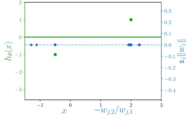
(b) End of first phase (Iteration $4000$)

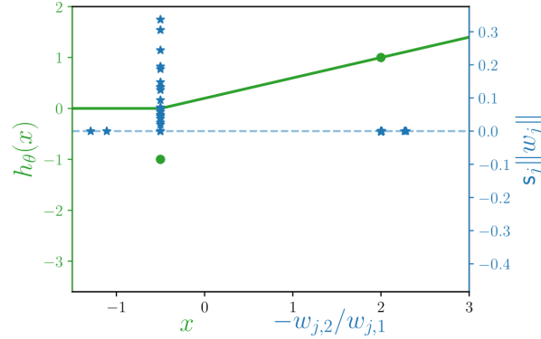
(c) End of second phase (Iteration $8000$)

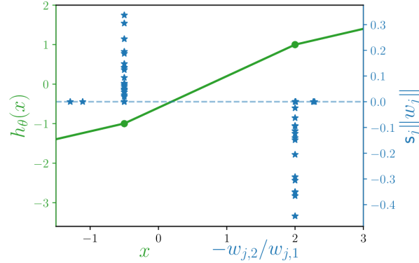
(d) End of third phase (Iteration $15000$)

Figure 2: State of training at different stages. The green dots correspond to the data, while the green line is the estimated function $h_{\theta}$. Each blue star represents a neuron $w_{j}$: its $x$-axis value is given by $-w_{j,2}/w_{j,1}$, which coincides with the position of the kink of its associated ReLU; its $y$-axis value is given by $\mathsf{s}_{j}\|w_{j}\|$, which we recall is the associated value of the output layer.

Figure 2 shows the training dynamics on this example. In particular, the state of the network is shown at different steps. In Figure 2(a), all the neurons are close to $0$ at initialisation. Figure 2(b) shows the end of the first phase, where the neurons are aligned towards two key directions. After the second phase, shown in Figure 2(c), all the neurons aligned with $D_{+}$ have grown in norm and the positive label is perfectly fitted. Similarly at the end of third phase in Figure 2(d), all neurons aligned with $-D_{-}$ have grown in norm and the negative label is fitted.

At the end of training, the loss is $0$ and the estimated function is simple. In particular, it only has two kinks, which illustrates the sparsity induced by the implicit bias. Also, the final estimated function might be counter-intuitive. Previous works on implicit bias indeed conjectured that the learned estimator is linear if the data can be linearly fitted (Kalimeris et al., 2019; Lyu et al., 2021). However, the learned function in Figure 2(d) has a smaller $\mathcal{F}_{1}$-norm than the linear interpolator.

Figure 3 shows the evolution of the loss during training. The saddle to saddle dynamics is well observed here: the parameters vector starts from the $0$ saddle point at initialisation and needs $5000$ iterations to leave this first saddle. A second saddle is then encountered at the end of the second phase and the trajectory only leaves this saddle around iteration $11000$, once the norm of the neurons in $S_{-,1}$ start being significant during the third phase. All these different experiments confirm 1 and the precise dynamics described in Section 4. Moreover, such training phenomena are not specific to the orthogonal data case, as observed in Appendix A.

Figure 3: Evolution of the training loss.

6 Conclusion and perspectives

We have shown that the training of non-linear neural networks on orthogonal data presents a rich dynamics with a small and omnidirectional intialisation. Convergence holds generically despite a truly non-convex landscape and the limit enjoys an implicit bias as a minimum $\ell_{2}$ parameter norm. Obviously, removing the orthogonal assumption on the inputs, while keeping a fine level of description is a major, but difficult, perspective for future work. Another key point to better understand the good generalisation of neural networks is to analyse the properties of the functions solving the minimum variation norm problem stated in Equation 8.

Appendix

Appendix A Additional experiments

A.1 Unidimensional data

This section presents additional experiments in the general setting where data are non-orthogonal. To be able to visualize the results, similarly to Section 5, we consider unidimensional data with a bias term, but with $5$ data points. Here again, we consider a neural network of width $m=60$ and run gradient descent with step size $10^{-3}$.

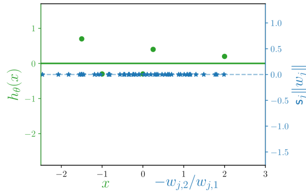
(a) Initialisation (Iteration $0$)

(b) End of early alignment (Iteration $15000$)

(c) Intermediate saddle (Iteration $94000$)

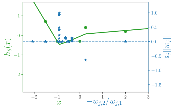
(d) Simultaneous norm growth and realignment (Iteration $150000$)

(e) Final state (Iteration $300000$)

(f) Loss profile

Figure 4: State of training at different stages and loss profile.

Similarly to Figure 2, Figure 4 presents the training dynamics with a small initialisation ($\lambda=\frac{10^{-4}}{\sqrt{m}}$). As in the orthogonal case, we first observe an early alignment phase in Figure 4(b). Afterwards, two groups of neurons (against a single group in the orthogonal case) grow in norms until reaching an intermediate saddle point in Figure 4(c). Note that during this norm-growth phase, the group of neurons does not remain aligned with a fixed direction, but changed in direction. A similar phenomenon happens when leaving the intermediate saddle point in Figure 4(d): the norm of these neurons still grow but they also change their direction. This behavior is what makes the general case fundamentally harder to analyse than the orthogonal one, where such a behavior does not happen. We believe that controlling this type of behavior is the key towards dealing with the general set up.

In Figure 4(e), we have a zero training loss and as in the orthogonal case, the estimated function is sparse in its number of kinks. Figure 4(f) shows that a saddle to saddle dynamics also happens in this general setup.

(a) Initialisation (Iteration $0$)

(b) End of training (Iteration $5000$)

Figure 5: Training dynamics for large initialisation.

Figure 5 on the other hand studies the impact of the initialisation scale. In particular, it shows the training dynamics for a large scale of initialisation ($\lambda=\frac{10}{\sqrt{m}}$). By comparing Figures 5(a) and 5(b), we indeed observe the lazy regime [Chizat et al., 2019]: the neuron weights do not significantly move between the initialisation and the end of training.

The final estimated function is not as simple as for small initialisation: it is approximately the interpolator coming from the Neural Tangent Kernel at initialisation, whose associated RKHS is described in Bietti and Mairal [2019]. The strong biased induced by initialisation and the poor generalising properties of this kernel interpolator illustrate the benefits of the rich regime obtained for small initialisation. However, this large initialisation has the advantage of converging towards $0$ loss much faster: the trajectory indeed does not go through saddle points that might significantly slow down the learning process. Similar results are observed for large initialisations when either considering unbalanced initialisation or orthogonal data.

A.2 High dimensional data

(a) Initialisation (Iteration $0$)

(b) End of alignment phase (Iteration $40000$)

(c) Growth of first cluster (Iteration $80000$)

(d) Final state (Iteration $200000$)

Figure 6: State of training at different stages. Each red (resp. purple) star represents a single neuron with $\mathsf{s}_{j}=-1$ (resp. $\mathsf{s}_{j}=1$): it shows (in polar coordinates) the projection of the hidden layer weight onto the $2$ dimensional space spanned by the two principal components of the hidden layer weights at the final state of training. The inner circle corresponds to $0$ norm vectors, whose direction is given by the angle.

(a) Loss profile

(b) Explained variance ratios of the principal components analysis of the final hidden weights

Figure 7: Additional information on the high dimensional experiment.

This section presents additional experiments for high dimensional, nearly orthogonal data. We generated $n=75$ data points $x_{i}$ drawn independently at random according to a standard Gaussian distribution of dimension $d=150$. It is then known that such points are almost orthogonal with large probability. The labels $y_{i}$ are then given by a $6$-neurons teacher network, whose weights were drawn at random following a Gaussian distribution.

From there, we trained a neural network with width $m=200$ (without bias terms), an initialisation scale $\lambda=\frac{10^{-20}}{\sqrt{md}}$ and a gradient step size of $10^{-3}$. Figure 6 illustrates the training dynamics of the parameters when projected onto the $2$ dimensional space of the two principal components of the $200\times 150$ matrix associated to the hidden layer of the network.

The training loss profile is given by Figure 7(a). Figure 7(b) finally shows the explained variance ratio of the principal components of the PCA used in Figure 6.

Behaviors close to the orthogonal case can easily be observed here. First, we can see in Figure 7(a) that the training loss converges to $0$ and that the dynamics goes through an intermediate saddle point around iteration $75000$. Also, thanks to Figure 6, we see the training dynamics (at least when projected onto the $2$ dimensional space of the two principal components) follows similar phases. At first, we observe an early alignment phase where the neurons align towards two key directions. During a second phase, a first cluster of neurons grows in norm while keeping a fixed direction. During a third phase, the same happens for the other cluster of neurons. Only after these three phases, the neurons will slightly move from these two key directions and reach the final state of Figure 6(d), for which we see that the neurons are not exactly aligned with two directions.

This last state is what differs from the exactly orthogonal case, where the final solution consists of a $2$ neurons network. This is obviously not the case here, as can be seen from Figure 6(d), but also from the explained variance ratios given in Figure 7(b). Indeed, we can there see that $80\%$ of the final state neurons are explained by the two principal components. This implies that the estimated interpolator is close to a $2$ neurons network, but still far from being only represented by $2$ direction (around $20\%$ of its variance is explained by the remaining directions).

Note that we here chose a very small initialisation scale (of order $10^{-20}$). As explained in Section 3.2, this confirms the exponential dependence of $\lambda$ in the number of data points and is merely needed to observe a clear saddle point in the dynamics, but similar final states of training are observed for much larger values initialisation scales.

Appendix B Main proofs

In this section, we prove the main theorem. Sections B.1 and B.2 provide additional notations and recall the assumption on the initialisation. Then, each subsection corresponds to the study of the different phases of the dynamics: Sections B.3, B.4, B.5 and B.6 prove respectively the alignment phase, the positive, then negative label fitting phases and finally the convergence phase.

B.1 Additional notations

First, we introduce the following additional notations. We need to define the two dynamical vectors that encode respectively the fitting of positive and negative labels

$$D_{+}^{t}=-\frac{1}{n}\sum_{k\mid y_{k}>0}(h_{\theta^{t}}(x_{k})-y_{k})x_{k}\quad\textrm{ and }\quad D_{-}^{t}=-\frac{1}{n}\sum_{k\mid y_{k}<0}(h_{\theta^{t}}(x_{k})-y_{k})x_{k}.$$

We also define the following open subsets of $\mathbb{R}^{d}$:

$$S_{+}=\{w\in\mathbb{R}^{d}\mid\forall k,\mathds{1}_{\langle w,x_{k}\rangle\geq 0}\geq\mathds{1}_{y_{k}>0}\}\quad\textrm{ and }\quad S_{-}=\{w\in\mathbb{R}^{d}\mid\forall k,\mathds{1}_{\langle w,x_{k}\rangle\geq 0}\geq\mathds{1}_{y_{k}<0}\}.$$

Note that $D_{+}\in S_{+}$ and $-D_{-}\in S_{-}$ and that neurons defined in Equations 5 and 6 correspond to

$$S_{+,1}=\{j\in\llbracket m\rrbracket\mid w_{j}^{0}\in S_{+}\text{ and }\mathsf{s}_{j}=1\}\quad\textrm{ and }\quad S_{-,1}=\{j\in\llbracket m\rrbracket\mid w_{j}^{0}\in S_{-}\text{ and }\mathsf{s}_{j}=-1\}.$$

B.2 Initialisation and assumptions on the dataset

We recall here, for the sake of completeness, the setup at initialisation. We initialise the dynamics on a balanced fashion: $a_{j}^{0}=\mathsf{s}_{j}\|w_{j}^{0}\|$. We take $\lambda>0$ and assume that $w_{j}^{0}=\lambda g_{j}$, where each $g_{j}\sim\mathcal{N}(0,I_{d})$ is an independent standard Gaussian. We assume that both $S_{+,1}$ and $S_{-,1}$ are non-empty and that for all $k$, $y_{k}\neq 0$. We also assume without loss of generality that $\|D_{+}\|>\|D_{-}\|$. This makes $r=\|D_{+}\|/\|D_{-}\|>1$. We fix $\varepsilon>0$ small enough so that

$$(1+3\varepsilon)\max\left(1-\alpha,\frac{\|D_{-}\|}{\|D_{+}\|}\right)\leq 1-\varepsilon\quad\text{and}\quad(1+3r\varepsilon)(1-\beta)\leq 1-\varepsilon$$

$$\text{where}\quad\alpha=\min_{k\mid y_{k}>0}\frac{y_{k}^{2}}{2\|D_{+}\|^{2}},\quad\beta=\min_{k\mid y_{k}<0}\frac{y_{k}^{2}}{2\|D_{-}\|^{2}}.$$

We finally introduce an arbitrarily small $\lambda_{*}>0$ that only depends on the training set $(x_{k},y_{k})_{k}$ and set $c=\max_{j\in\llbracket m\rrbracket}\|w_{j}^{0}\|/\lambda=\max_{j\in\llbracket m\rrbracket}\|g_{j}\|$.

Because of the non-differentiability of the ReLU activation, the gradient flow is not uniquely defined. In the orthogonal case, we have in particular the following ODE

$$\frac{\mathrm{d}\langle w_{j}^{t},x_{k}\rangle}{\mathrm{d}t}=-\frac{h_{\theta^{t}}(x_{k})-y_{k}}{n}\|w_{j}^{t}\|\mathds{1}_{\langle w_{j}^{t},x_{k}\rangle>0},$$ (11)

which leads to the following key lemma.

Lemma 6.

For any $t^{\prime}\geq t$, $j\in\llbracket m\rrbracket$ and $k\in[n]$:

$$\mathds{1}_{\langle w_{j}^{t},x_{k}\rangle<0}\implies\mathds{1}_{\langle w_{j}^{t^{\prime}},x_{k}\rangle<0}.$$

Proof.

This is a direct consequence of Equation 11. ∎

B.3 Phase 1: proof of Lemma 2

During the first phase, the neurons remain small in norm and they move tangentially to align with the vectors $D_{+}$ and $D_{-}$. The duration of this movement is typically sub-logarithmic in $\lambda$, the initialisation scale. As $\|D_{+}\|>\|D_{-}\|$, neurons in $S_{+,1}$ move slightly faster to align with $D_{+}$ than the ones in $S_{-,1}$ that align with $-D_{-}$. We begin by describing the dynamics of neurons in $S_{+,1}$ in Lemma 7 and derive similar results for the one of $S_{-,1}$ in Lemma 8. These two Lemmas constitute together Lemma 2 of the main text.

First, we define the following ending time of the phase $+1$:

$$t_{+1}=\frac{-\varepsilon\ln(\lambda)}{\|D_{+}\|}.$$ (12)

We have the following lemma.

Lemma 7 (Phase $+1$).

If $\lambda\leq\lambda_{*}$, then we have the following inequalities,

1. $\forall j\in\llbracket m\rrbracket,\|w_{j}^{t_{+1}}\|\leq 2c\lambda^{1-\varepsilon}$

2. $\forall j\in S_{+,1},\langle\mathsf{w}_{j}^{t_{+1}},D_{+}\rangle\geq(1-2\lambda^{\varepsilon})\|D_{+}\|$.

3. For all $j\in S_{+,1}$, let $k$ such that $y_{k}<0$, then $\langle w_{j}^{t_{+1}},x_{k}\rangle=0$.

The condition (i) of the lemma means that the neurons do not grow so much in this first phase, whereas (ii) states that they have aligned with vectors $D_{+}$. Finally (iii) shows that neurons in $S_{+,1}$ deactivate along negative labels during this first phase.

Proof.

We divide the proof in three steps. First one is to control the growth of the neurons norm until $t_{+1}$. The second step shows that the tangential movement is faster, while the third one shows that neurons in $S_{+,1}$ “unalign” with the directions of negative labels.

First step: we show (i), i.e. that for $t\leq t_{+1}$, we have $\|w_{j}^{t}\|\leq 2c\lambda^{1-\varepsilon}$. Note first that, thanks to the balancedness, $a_{j}^{t}=\mathsf{s}_{j}\|w_{j}^{t}\|$. Let $\tau_{\lambda}:=\inf\{t\geq 0\mid\exists j\in\llbracket m\rrbracket,\|w_{j}^{t}\|>2c\lambda^{1-\varepsilon}\}$, then for all $t\leq\tau_{\lambda}$, we have $\|w_{j}^{t}\|\leq 2c\lambda^{1-\varepsilon}$ and hence,

$$\left|h_{\theta^{t}}(x_{k})\right|\leq\sum_{j=1}^{m}\|w_{j}^{t}\||\sigma(\langle w_{j},x_{k}\rangle)|\leq\sum_{j=1}^{m}\|w_{j}^{t}\|^{2}\leq 4mc^{2}\lambda^{2(1-\varepsilon)}.$$

Then, for $\lambda_{*}$ such that $\lambda_{*}^{2(1-\varepsilon)}\leq\frac{\min_{k}|y_{k}|}{4mc^{2}}$, $y_{k}-h_{\theta^{t}}(x_{k})$ and $y_{k}$ have the same sign for any $t\leq\tau_{\lambda}$. As a consequence, for $j$ such that $\mathsf{s}_{j}=1$, Equation 3 yields

$$\frac{\mathrm{d}\|w_{j}^{t}\|}{\mathrm{d}t} =\frac{1}{n}\sum_{\begin{subarray}{c}k|\langle x_{k},w_{j}^{t}\rangle>0\end{subarray}}\left(y_{k}-h_{\theta^{t}}(x_{k})\right)\langle x_{k},w_{j}^{t}\rangle\leq\frac{1}{n}\sum_{\begin{subarray}{c}k\mid\langle x_{k},w_{j}^{t}\rangle>0\end{subarray}}\left(y_{k}-h_{\theta^{t}}(x_{k})\right)\langle x_{k},w_{j}^{t}\rangle\mathds{1}_{y_{k}>0}.$$

Now, denote $\displaystyle D^{t}_{+,j}:=\frac{1}{n}\sum_{\begin{subarray}{c}k\mid\langle x_{k},w_{j}^{t}\rangle>0\end{subarray}}\left(y_{k}-h_{\theta^{t}}(x_{k})\right)x_{k}\mathds{1}_{y_{k}>0}$, we have

$$\langle D^{t}_{+,j},w_{j}^{t}\rangle \leq\|D^{t}_{+,j}\|\|w_{j}^{t}\|\leq\|D^{t}_{+}\|\|w_{j}^{t}\|\leq(\|D_{+}\|+\|\frac{1}{n}\sum_{k,y_{k}>0}h_{\theta^{t}}(x_{k})x_{k}\|)\|w_{j}^{t}\|$$

$$\leq(\|D_{+}\|+4mc^{2}\lambda^{2(1-\varepsilon)})\|w_{j}^{t}\|.$$

The same series of inequalities holds in the case $\mathsf{s}_{j}=-1$ for $\|D_{-}^{t}\|$. Overall,

$$\frac{\mathrm{d}\|w_{j}^{t}\|}{\mathrm{d}t} \leq\left(\max\left\{\|D_{+}\|,\|D_{-}\|\right\}+4mc^{2}\lambda^{2(1-\varepsilon)}\right)\|w_{j}^{t}\|$$

$$\leq\left(\|D_{+}\|+4mc^{2}\lambda^{2(1-\varepsilon)}\right)\|w_{j}^{t}\|.$$

By Grönwall’s lemma, this gives for any $t\leq\tau_{\lambda}$, $\|w_{j}^{t}\|\leq\|w_{j}^{0}\|e^{\left(\|D_{+}\|+4mc^{2}\lambda^{2(1-\varepsilon)}\right)t}$. This shows that for $t\leq\min(\tau_{\lambda},t_{+1})$,

$$\|w_{j}^{t}\|\leq c\lambda^{1-\varepsilon}e^{\frac{-4\varepsilon mc^{2}\lambda^{2(1-\varepsilon)}}{\|D_{+}\|}\ln(\lambda)}<2c\lambda^{1-\varepsilon},$$ (13)

where $\lambda^{*}$ has been taken small enough. Hence $\tau_{\lambda}\geq t_{+1}$.

Second step: we show condition (ii). Indeed, let us now choose any $j\in S_{+,1}$. We have the following decomposition:

$$D_{j}^{t}=D_{+}-\frac{1}{n}\sum_{\begin{subarray}{c}k\mid\langle x_{k},w_{j}^{t}\rangle>0\end{subarray}}h_{\theta^{t}}(x_{k})x_{k}\mathds{1}_{y_{k}>0}+D_{-,j}^{t},$$

so that as all vectors in the $D_{-,j}^{t}$ are different from the one of $D_{+}$, by orthogonality we have,

$$\langle D_{j}^{t},D_{+}\rangle=\|D_{+}\|^{2}-\frac{1}{n}\sum_{\begin{subarray}{c}k\mid\langle x_{k},w_{j}^{t}\rangle>0\end{subarray}}h_{\theta^{t}}(x_{k})\langle x_{k},D_{+}\rangle\mathds{1}_{y_{k}>0}.$$

Now, let us analyse the tangential movement for these $j$’s: for all $t\leq t_{+1}$, Equation 9 leads to the following growth comparison

$$\frac{\mathrm{d}\langle\mathsf{w}_{j}^{t},D_{+}\rangle}{\mathrm{d}t} =\langle D^{t}_{j},D_{+}\rangle-\langle D^{t}_{j},\mathsf{w}_{j}^{t}\rangle\langle\mathsf{w}_{j}^{t},D_{+}\rangle$$

$$=\|D_{+}\|^{2}-\langle\mathsf{w}_{j}^{t},D_{+}\rangle^{2}-\frac{1}{n}\sum_{\begin{subarray}{c}k\mid\langle x_{k},w_{j}^{t}\rangle>0\end{subarray}}h_{\theta^{t}}(x_{k})\langle x_{k},D_{+}-\langle D_{+},\mathsf{w}_{j}^{t}\rangle\mathsf{w}_{j}^{t}\rangle\mathds{1}_{y_{k}>0}-\langle D^{t}_{j,-},\mathsf{w}_{j}^{t}\rangle\langle\mathsf{w}_{j}^{t},D_{+}\rangle,$$

and as we have, $-\langle D^{t}_{j,-},\mathsf{w}_{j}^{t}\rangle\langle\mathsf{w}_{j}^{t},D_{+}\rangle\geq 0$ and the third term lower bounded by $-4mc^{2}\|D_{+}\|\lambda^{2(1-\varepsilon)}$, it yields

$$\frac{\mathrm{d}\langle\mathsf{w}_{j}^{t},D_{+}\rangle}{\mathrm{d}t} \geq\|D_{+}\|^{2}-4mc^{2}\|D_{+}\|\lambda^{2(1-\varepsilon)}-\langle\mathsf{w}_{j}^{t},D_{+}\rangle^{2}.$$ (14)

Solutions of the ODE $f^{\prime}(t)=a^{2}-f^{2}(t)$ with value in $(-a,a)$ are of the form $f(t)=a\tanh(a(t+t_{0}))$ for some $t_{0}$. Note in the remaining of the proof $a^{2}=\|D_{+}\|^{2}-4mc^{2}\|D_{+}\|\lambda^{2(1-\varepsilon)}$. In our case, define $t_{0}$ such that $\langle\mathsf{w}_{j}^{0},D_{+}\rangle=a\tanh(at_{0})$, then, by Grönwall comparison, it yields:

$$\langle\mathsf{w}_{j}^{t},D_{+}\rangle\geq a\tanh(a(t+t_{0})).$$

Note that $\langle\mathsf{w}_{j}^{0},D_{+}\rangle\geq 0$, so that $t_{0}\geq 0$. As a consequence, we simply have

$$\langle\mathsf{w}_{j}^{t},D_{+}\rangle\geq a\tanh(at).$$

Now, using the inequality $\tanh(x)\geq 1-2e^{-2x}$, we have

$$\langle\mathsf{w}_{j}^{t_{+1}},D_{+}\rangle \geq a(1-2e^{2a\frac{\varepsilon}{\|D_{+}\|}\ln(\lambda)}).$$

We have the following inequalities on $a$ when choosing $\lambda_{*}$ small enough:

$$a=\sqrt{\|D_{+}\|^{2}-4mc^{2}\|D_{+}\|\lambda^{2(1-\varepsilon)}}\geq\frac{3\|D_{+}\|}{4}.$$

This leads for any $j\in S_{+,1}$ and $\lambda^{*}$ small enough to

$$\langle\mathsf{w}_{j}^{t_{+1}},D_{+}\rangle >(\|D_{+}\|-2c\sqrt{m\|D_{+}\|}\lambda^{1-\varepsilon})\left(1-2\lambda^{\frac{3\varepsilon}{2}}\right)$$

$$>\|D_{+}\|\left(1-2\lambda^{\frac{3\varepsilon}{2}}\right)-2c\sqrt{m\|D_{+}\|}\lambda^{1-\varepsilon}$$

$$>\|D_{+}\|\left(1-2\lambda^{\varepsilon}\right),$$

which proves condition (ii).

Third step: we show (iii). Consider $j\in S_{+,1}$ and $k$ such that $y_{k}<0$. If $\langle w_{j}^{0},x_{k}\rangle<0$, then by Lemma 6, there is nothing to prove. Otherwise, as for $t\leq t_{+1}$ we have $\|w_{j}^{t}\|\leq 2c\lambda^{1-\varepsilon}$, it yields (as long as $\langle\mathsf{w}_{j}^{t},x_{k}\rangle>0$)

$$\frac{\mathrm{d}}{\mathrm{d}t}\langle\mathsf{w}_{j}^{t},x_{k}\rangle =\langle D_{j}^{t},x_{k}\rangle-\langle D_{j}^{t},\mathsf{w}_{j}^{t}\rangle\langle\mathsf{w}_{j}^{t},x_{k}\rangle$$

$$=\frac{1}{n}(y_{k}-h_{\theta}(x_{k}))-\frac{1}{n}\langle\mathsf{w}_{j}^{t},x_{k}\rangle\sum_{l\mid\langle\mathsf{w}_{j}^{t},x_{l}\rangle>0}(y_{l}-h_{\theta}(x_{l}))\langle\mathsf{w}_{j}^{t},x_{l}\rangle<0.$$

Hence, if for some time $\tau\leq t_{+1}$, we have $\langle\mathsf{w}_{j}^{\tau},x_{k}\rangle=0$, then for all times $t\in[\tau,t_{+1}]$, this quantity remains $0$. We now continue to upperbound the derivative of $\langle\mathsf{w}_{j}^{\tau},x_{k}\rangle$:

$$\frac{\mathrm{d}}{\mathrm{d}t}\langle\mathsf{w}_{j}^{t},x_{k}\rangle \leq\frac{1}{n}(y_{k}+4mc^{2}\lambda^{2(1-\varepsilon)})-\frac{1}{n}\langle\mathsf{w}_{j}^{t},x_{k}\rangle\sum_{l\mid\langle\mathsf{w}_{j}^{t},x_{l}\rangle>0}(y_{l}-4mc^{2}\lambda^{2(1-\varepsilon)})\langle\mathsf{w}_{j}^{t},x_{l}\rangle$$

$$\leq\frac{y_{k}}{n}-\frac{1}{n}\langle\mathsf{w}_{j}^{t},x_{k}\rangle\sum_{l\mid\langle\mathsf{w}_{j}^{t},x_{l}\rangle>0}y_{l}\langle\mathsf{w}_{j}^{t},x_{l}\rangle\mathds{1}_{y_{l}<0}+5mc^{2}\lambda^{2(1-\varepsilon)}.$$

From this, we sum all the $y_{k}<0$, and noting $\displaystyle f(t):=-\frac{1}{n}\!\!\sum_{k\mid\langle\mathsf{w}_{j}^{t},x_{k}\rangle>0}\!\!\!\!y_{k}\langle\mathsf{w}_{j}^{t},x_{k}\rangle\mathds{1}_{y_{k}<0}$, we have

$$\frac{\mathrm{d}}{\mathrm{d}t}f(t)\leq-\frac{1}{n^{2}}\sum_{k\mid y_{k}<0}y^{2}_{k}+f(t)^{2}-5mc^{2}\lambda^{2(1-\varepsilon)}\frac{1}{n}\sum_{k\mid y_{k}<0}y_{k}.$$

If we let $a^{2}:=\frac{1}{n^{2}}\sum_{k\mid y_{k}<0}y^{2}_{k}+5mc^{2}\lambda^{2(1-\varepsilon)}\frac{1}{n}\sum_{k\mid y_{k}<0}y_{k}>0$, we have $f^{\prime}(t)\leq-a^{2}+f(t)^{2}$, and as by Cauchy-Schwarz

$$f(0)^{2} \leq\frac{1}{n^{2}}\sum_{k\mid\langle\mathsf{w}_{j}^{0},x_{k}\rangle>0}y_{k}^{2}\mathds{1}_{y_{k}<0}\sum_{k\mid\langle\mathsf{w}_{j}^{0},x_{k}\rangle>0}\langle\mathsf{w}_{j}^{0},x_{k}\rangle^{2}\mathds{1}_{y_{k}<0}$$

$$=\frac{1}{n^{2}}\left(\sum_{k\mid\langle\mathsf{w}_{j}^{0},x_{k}\rangle>0}y_{k}^{2}\mathds{1}_{y_{k}<0}\right)\left(\|\mathsf{w}_{j}^{0}\|^{2}-\sum_{k}\langle\mathsf{w}_{j}^{0},x_{k}\rangle^{2}\left(\mathds{1}_{y_{k}>0}\mathds{1}_{\langle\mathsf{w}_{j}^{0},x_{k}\rangle>0}+\mathds{1}_{\langle\mathsf{w}_{j}^{0},x_{k}\rangle<0}\right)\right)$$

$$<\left(a^{2}+\lambda^{1-2\varepsilon}\right)\left(1-\sum_{k}\langle\mathsf{w}_{j}^{0},x_{k}\rangle^{2}\left(\mathds{1}_{y_{k}>0}\mathds{1}_{\langle\mathsf{w}_{j}^{0},x_{k}\rangle>0}+\mathds{1}_{\langle\mathsf{w}_{j}^{0},x_{k}\rangle<0}\right)\right)$$

$$<a^{2},$$

where the two last inequalities are valid for $\lambda$ small enough. Hence $t\mapsto f(t)$ is decreasing and $f^{\prime}(t)\leq-a^{2}+f(0)^{2}$, that is if we call $b:=a^{2}-f(0)^{2}>0$, we have $f(t)\leq-bt+f(0)$, and for $\tau=f(0)/b$, we have $f(\tau)=0$. And as $\tau<t_{+1}$, we have $f(t_{+1})=0$. This concludes the proof of condition (iii) and of the lemma. ∎

Now, we show that the exact same conclusion is also valid for the neurons in $S_{-,1}$ i.e., after a sub-logarithmic time, they eventually align with $-D_{-}$ and deactivates with respect to positive outputs. We define here a ending time similar to (12):

$$t_{-1}=\frac{-\varepsilon r\ln(\lambda)}{\|D_{+}\|}.$$ (15)

We prove the following lemma analogous to Lemma 7.

Lemma 8 (Phase $-1$).

If $\lambda\leq\lambda_{*}$, then we have the following inequalities,

1. $\forall j\in\llbracket m\rrbracket,\|w_{j}^{t_{-1}}\|\leq 2c\lambda^{1-r\varepsilon}$

2. $\forall j\in S_{-,1},\langle\mathsf{w}_{j}^{t_{-1}},-D_{-}\rangle\geq(1-2\lambda^{\varepsilon})\|D_{-}\|$.

3. For all $j\in S_{-,1}$, let $k$ such that $y_{k}>0$, then $\langle w_{j}^{t_{-1}},x_{k}\rangle=0$.

Proof.

The proof is essentially the same than the proof of Lemma 7. We will be short and underline solely the main differences.

First step: we show condition (i), i.e. that for $t\leq t_{-1}$, we have $\|w_{j}^{t}\|\leq 2c\lambda^{1-r\varepsilon}$. Indeed, let $\tau^{r}_{\lambda}:=\inf\{t\geq 0\mid\exists j\in\llbracket m\rrbracket,\|w_{j}^{t}\|>2c\lambda^{1-r\varepsilon}\}$. For all $t\leq\tau^{r}_{\lambda}$, we have $\left|h_{\theta^{t}}(x_{k})\right|\leq 4mc^{2}\lambda^{2(1-r\varepsilon)}$ and similarly to the proof of Lemma 7, we have that for $t\leq\tau^{r}_{\lambda}$, $\|w_{j}^{t}\|\leq\|w_{j}^{0}\|e^{\left(\|D_{+}\|+4mc^{2}\lambda^{2(1-r\varepsilon)}\right)t}$. This shows that for $t\leq\min(\tau^{r}_{\lambda},\,t_{-1})$,

$$\|w_{j}^{t}\|\leq c\lambda^{1-r\varepsilon}e^{\frac{-4\varepsilon mc^{2}\lambda^{2(1-r\varepsilon)}}{\|D_{+}\|}\ln(\lambda)}<2c\lambda^{1-r\varepsilon},$$ (16)

where $\lambda^{*}$ has been taken small enough. Hence $\tau^{r}_{\lambda}\geq t_{-1}$.

Second step: we show (ii), i.e. that the neurons almost align after time $t_{-1}$. Indeed, for $j\in S_{-,1}$, similarly to Lemma 7, we have that for all $t\leq t_{-1}$:

$$\frac{\mathrm{d}\langle\mathsf{w}_{j}^{t},-D_{-}\rangle}{\mathrm{d}t}\geq\|D_{-}\|^{2}-4mc^{2}\|D_{-}\|\lambda^{2(1-r\varepsilon)}-\langle\mathsf{w}_{j}^{t},D_{-}\rangle^{2}.$$

Denoting $a_{r}^{2}=\|D_{-}\|^{2}-4mc^{2}\|D_{-}\|\lambda^{2(1-r\varepsilon)}$, we have by Grönwall comparison

$$\langle\mathsf{w}_{j}^{t},-D_{-}\rangle\geq a_{r}\tanh(a_{r}t).$$

Now, this gives $\langle\mathsf{w}_{j}^{t_{-1}},-D_{-}\rangle>a_{r}(1-2e^{2a_{r}\frac{r\varepsilon}{\|D_{+}\|}\ln(\lambda)})$ and lower bounding $a_{r}$ as before, we have

$$\langle\mathsf{w}_{j}^{t_{-1}},-D_{-}\rangle>\|D_{-}\|\left(1-2\lambda^{\varepsilon}\right),$$

and this shows the condition (ii).

Third step: we show (iii). Consider $j\in S_{-,1}$ and $k$ such that $y_{k}>0$. If $\langle w_{j}^{0},x_{k}\rangle<0$, then by Lemma 6, there is nothing to prove. Otherwise, as for $t\leq t_{-1}$ we have $\|w_{j}^{t}\|\leq 2c\lambda^{1-r\varepsilon}$, it yields (as long as $\langle\mathsf{w}_{j}^{t},x_{k}\rangle>0$)

$$\frac{\mathrm{d}}{\mathrm{d}t}\langle\mathsf{w}_{j}^{t},x_{k}\rangle =-\langle D_{j}^{t},x_{k}\rangle+\langle D_{j}^{t},\mathsf{w}_{j}^{t}\rangle\langle\mathsf{w}_{j}^{t},x_{k}\rangle$$

$$=\frac{1}{n}(h_{\theta}(x_{k})-y_{k})-\frac{1}{n}\langle\mathsf{w}_{j}^{t},x_{k}\rangle\sum_{l\mid\langle\mathsf{w}_{j}^{t},x_{l}\rangle>0}(h_{\theta}(x_{l})-y_{l})\langle\mathsf{w}_{j}^{t},x_{l}\rangle<0.$$

Hence, if for some time $\tau\leq t_{-1}$, we have $\langle\mathsf{w}_{j}^{\tau},x_{k}\rangle=0$, then for all times $t\in[\tau,t_{-1}]$, this quantity will remain $0$. We now we continue to upperbound the derivative of $\langle\mathsf{w}_{j}^{\tau},x_{k}\rangle$:

$$\frac{\mathrm{d}}{\mathrm{d}t}\langle\mathsf{w}_{j}^{t},x_{k}\rangle \leq\frac{1}{n}(4mc^{2}\lambda^{2(1-r\varepsilon)}-y_{k})-\frac{1}{n}\langle\mathsf{w}_{j}^{t},x_{k}\rangle\sum_{l\mid\langle\mathsf{w}_{j}^{t},x_{l}\rangle>0}(-4mc^{2}\lambda^{2(1-r\varepsilon)}-y_{l})\langle\mathsf{w}_{j}^{t},x_{l}\rangle$$

$$\leq-\frac{y_{k}}{n}+\frac{1}{n}\langle\mathsf{w}_{j}^{t},x_{k}\rangle\sum_{l\mid\langle\mathsf{w}_{j}^{t},x_{l}\rangle>0}y_{l}\langle\mathsf{w}_{j}^{t},x_{l}\rangle\mathds{1}_{y_{l}>0}+5mc^{2}\lambda^{2(1-r\varepsilon)}.$$

From this, we sum all the $y_{k}>0$, and noting $\displaystyle f(t):=\frac{1}{n}\!\!\sum_{k\mid\langle\mathsf{w}_{j}^{t},x_{k}\rangle>0}\!\!\!\!y_{k}\langle\mathsf{w}_{j}^{t},x_{k}\rangle\mathds{1}_{y_{k}>0}$, we have

$$\frac{\mathrm{d}}{\mathrm{d}t}f(t)\leq-\frac{1}{n^{2}}\sum_{k\mid y_{k}>0}y^{2}_{k}+f(t)^{2}+5mc^{2}\lambda^{2(1-r\varepsilon)}\frac{1}{n}\sum_{k\mid y_{k}>0}y_{k}.$$

If we let $a^{2}:=\frac{1}{n^{2}}\sum_{k\mid y_{k}>0}y^{2}_{k}-5mc^{2}\lambda^{2(1-r\varepsilon)}\frac{1}{n}\sum_{k\mid y_{k}>0}y_{k}>0$, we have $f^{\prime}(t)\leq-a^{2}+f(t)^{2}$, and as by Cauchy-Schwarz

$$f(0)^{2} \leq\frac{1}{n^{2}}\sum_{k\mid\langle\mathsf{w}_{j}^{0},x_{k}\rangle>0}y_{k}^{2}\mathds{1}_{y_{k}>0}\sum_{k\mid\langle\mathsf{w}_{j}^{0},x_{k}\rangle>0}\langle\mathsf{w}_{j}^{0},x_{k}\rangle^{2}\mathds{1}_{y_{k}>0}$$

$$<\frac{1}{n^{2}}\left(\sum_{k\mid\langle\mathsf{w}_{j}^{0},x_{k}\rangle>0}y_{k}^{2}\mathds{1}_{y_{k}>0}\right)\left(\|\mathsf{w}_{j}^{0}\|^{2}-\sum_{k}\langle\mathsf{w}_{j}^{0},x_{k}\rangle^{2}\left(\mathds{1}_{y_{k}<0}\mathds{1}_{\langle\mathsf{w}_{j}^{0},x_{k}\rangle>0}+\mathds{1}_{\langle\mathsf{w}_{j}^{0},x_{k}\rangle<0}\right)\right)$$

$$<\left(a^{2}+\lambda^{1-2\varepsilon}\right)\left(1-\sum_{k}\langle\mathsf{w}_{j}^{0},x_{k}\rangle^{2}\left(\mathds{1}_{y_{k}<0}\mathds{1}_{\langle\mathsf{w}_{j}^{0},x_{k}\rangle>0}+\mathds{1}_{\langle\mathsf{w}_{j}^{0},x_{k}\rangle<0}\right)\right)$$

$$<a^{2},$$

where the two last inequalities are valid for $\lambda$ small enough. Hence $t\mapsto f(t)$ is decreasing and $f^{\prime}(t)\leq-a^{2}+f(0)^{2}$, that is if we call $b:=a^{2}-f(0)^{2}>0$, we have $f(t)\leq-bt+f(0)$, and for $\tau=f(0)/b$, we have $f(\tau)=0$. And as $\tau<t_{-1}$, we have $f(t_{-1})=0$. This concludes the proof of condition (iii) and of the Lemma. ∎

We end this subsection by a lemma that shows that until $t_{\pm 1}$, the neurons $w^{t}_{j}$ with $j\in S_{\pm 1}$, could not have collapsed to $0$.

Lemma 9.

Define $\underline{c}=\min\|w_{j}^{0}\|/\lambda$, then, if $\lambda\leq\lambda^{*}$,

1. for all $t\leq t_{+1}$, $\forall j\in S_{+,1}$, $\displaystyle\|w_{j}^{t}\|>\underline{c}\lambda^{1+\varepsilon}/2$,

2. for all $t\leq t_{-1}$, $\forall j\in S_{-,1}$, $\displaystyle\|w_{j}^{t}\|>\underline{c}\lambda^{1+r\varepsilon}/2$.

Proof.

Let us begin with the first point. As stated in the proof of Lemma 7, $y_{k}-h_{\theta^{t}}(x_{k})$ and $y_{k}$ have the same sign for any $t\leq t_{+1}$. As a consequence, for $j\in S_{+,1}$, it yields

$$\frac{\mathrm{d}\|w_{j}^{t}\|}{\mathrm{d}t} \geq\langle D_{-,j}^{t},w_{j}^{t}\rangle\geq-\|D_{-,j}^{t}\|\|w_{j}^{t}\|\geq-\left(\|D_{-}\|+\|\frac{1}{n}\sum_{k,y_{k}<0}h_{\theta^{t}}(x_{k})x_{k}\|\right)\|w_{j}^{t}\|$$

$$\geq-\left(\|D_{+}\|+4mc^{2}\lambda^{2(1-\varepsilon)}\right)\|w_{j}^{t}\|.$$

Then, by Grönwall’s lemma, this gives for any $t\leq t_{+1}$, $\|w_{j}^{t}\|\geq\|w_{j}^{0}\|e^{-\left(\|D_{+}\|+4mc^{2}\lambda^{2(1-\varepsilon)}\right)t}$. This shows that, for $t\leq t_{+1}$,

$$\|w_{j}^{t}\|\geq\underline{c}\lambda^{1+\varepsilon}e^{\frac{4\varepsilon mc^{2}\lambda^{2(1-\varepsilon)}}{\|D_{+}\|}\ln(\lambda)}>\underline{c}\lambda^{1+\varepsilon}/2.$$

This concludes the first point of the lemma. The second point is very similar to the first one. Indeed, in this case also, for $t\leq t_{-1}$, $y_{k}$ rules the sign of the residual so that for $j\in S_{-,1}$,

$$\frac{\mathrm{d}\|w_{j}^{t}\|}{\mathrm{d}t} \geq\langle D_{+,j}^{t},w_{j}^{t}\rangle\geq-\|D_{+,j}^{t}\|\|w_{j}^{t}\|\geq-\left(\|D_{+}\|+\|\frac{1}{n}\sum_{k,y_{k}>0}h_{\theta^{t}}(x_{k})x_{k}\|\right)\|w_{j}^{t}\|$$

$$\geq-\left(\|D_{+}\|+4mc^{2}\lambda^{2(1-r\varepsilon)}\right)\|w_{j}^{t}\|.$$

Then, by Grönwall’s lemma, this gives for any $t\leq t_{-1}$, $\|w_{j}^{t}\|\geq\|w_{j}^{0}\|e^{-\left(\|D_{+}\|+4mc^{2}\lambda^{2(1-r\varepsilon)}\right)t}$. This shows that, as $t\leq t_{-1}$,

$$\|w_{j}^{t}\|\geq\underline{c}\lambda^{1+r\varepsilon}e^{\frac{4\varepsilon rmc^{2}\lambda^{2(1-r\varepsilon)}}{\|D_{+}\|}\ln(\lambda)}>\underline{c}\lambda^{1+r\varepsilon}/2.$$

This concludes the proof. ∎

B.4 Phase 2: proof of Lemma 3

During the second phase, the norm of the neurons in $S_{+,1}$ (which are aligned with $D_{+}$) grows until perfectly fitting all the positive labels of the training points. Meanwhile, all the other neurons do not move significantly. We define the ending time of the second phase as

$$t_{2}=\inf\Bigg{\{}t\geq t_{+1}\mid \text{ either }\exists j\not\in S_{+,1},\|w_{j}^{t}\|\geq 2c\lambda^{\varepsilon}$$ (17)

$$\text{or }\sum_{j\in S_{+,1}}\|w_{j}^{t}\|^{2}\geq n\|D_{+}\|-\lambda^{\frac{\varepsilon}{5}}$$

$$\text{or }\exists j\in S_{+,1},\langle\mathsf{w}_{j}^{t},D_{+}\rangle\leq\|D_{+}\|-\lambda^{\frac{\varepsilon}{2}}\Bigg{\}}.$$

The following lemma corresponds to Lemma 3 of the main text.

Lemma 10.

If $\lambda\leq\lambda_{*}$, then we have the following inequalities

1. $t_{2}\leq-\frac{1+3\varepsilon}{\|D_{+}\|}\ln(\lambda),$

2. $\forall j\in\llbracket m\rrbracket\setminus S_{+,1},\|w_{j}^{t_{2}}\|<2c\lambda^{\varepsilon},$

3. $\forall j\in S_{+,1},\langle\mathsf{w}_{j}^{t_{2}},D_{+}\rangle>\|D_{+}\|-\lambda^{\frac{\varepsilon}{2}}.$

The first point of the lemma states that the second phase lasts a time of order $-\ln(\lambda)$. The other two points state that the first and third conditions in the definition of $t_{2}$ do not hold at the end of the phase. Thus, the second condition in Equation 17 holds at $t_{2}$, meaning that the norm of the neurons in $S_{+,1}$ have grown enough to fit the positive labels:

$$\sum_{j\in S_{+,1}}\|w_{j}^{t_{2}}\|^{2}=n\|D_{+}\|-\lambda^{\frac{\varepsilon}{5}}$$

A direct consequence of this is that at the end of the second phase, the training loss on the positive labels is of order $\lambda^{\frac{2\varepsilon}{5}}$ (at least).

Proof.

Preliminaries: define for this proof $h(t)=\|D_{+}\|-\min_{j\in S_{+,1}}\langle\mathsf{w}_{j}^{t},D_{+}\rangle$. By definition of the second phase, we have $h(t)\leq\lambda^{\frac{\varepsilon}{2}}$ for any $t\in[t_{+1},t_{2}]$.

We first show that during the whole second phase, $D_{+}^{t}$ is almost colinear with $D_{+}$. For any $j\in S_{+,1}$ and $t\in[t_{+1},t_{2}]$, define $d_{j}^{t}=\mathsf{w}_{j}^{t}-\frac{D_{+}}{\|D_{+}\|}$. Since $\mathsf{w}_{j}^{t}$ and $\frac{D_{+}}{\|D_{+}\|}$ are both of norm $1$, we have $\|d_{j}^{t}\|^{2}=-2\langle d_{j}^{t},\frac{D_{+}}{\|D_{+}\|}\rangle$. By definition of $h(t)$,

$$0\geq\langle d_{j}^{t},D_{+}\rangle\geq-h(t).$$

So finally, we have for any $j\in S_{+,1}$ and $t\in[t_{+1},t_{2}]$ the decomposition

$$\mathsf{w}_{j}^{t}=\frac{D_{+}}{\|D_{+}\|}+d_{j}^{t}\qquad\text{with}\qquad\|d_{j}^{t}\|^{2}\leq 2\frac{h(t)}{\|D_{+}\|}.$$ (18)

Now let any $k$ such that $y_{k}>0$. Using Equation 18 and the fact that $\|w_{j}^{t}\|\leq 2c\lambda^{\varepsilon}$ for any $j\not\in S_{+,1}$, we have for any $t\in[t_{+1},t_{2}]$:

$$h_{\theta^{t}}(x_{k}) =\sum_{j\in S_{+,1}}\|w_{j}^{t}\|\langle w_{j}^{t},x_{k}\rangle+\sum_{j\not\in S_{+,1}}\mathsf{s}_{j}\|w_{j}^{t}\|\langle w_{j}^{t},x_{k}\rangle$$

$$=\sum_{j\in S_{+,1}}\frac{\|w_{j}^{t}\|^{2}}{\|D_{+}\|}\langle D_{+},x_{k}\rangle+\underbrace{\sum_{j\in S_{+,1}}\|w_{j}^{t}\|^{2}\langle d_{j}^{t},x_{k}\rangle+\sum_{j\not\in S_{+,1}}\mathsf{s}_{j}\|w_{j}^{t}\|\langle w_{j}^{t},x_{k}\rangle}$$

$$=\sum_{j\in S_{+,1}}\frac{\|w_{j}^{t}\|^{2}}{\|D_{+}\|}\langle D_{+},x_{k}\rangle+\hskip 85.35826pth_{k}(t),$$

where $\displaystyle|h_{k}(t)|\leq\sum_{j\in S_{+,1}}\|w_{j}^{t}\|^{2}|\langle d_{j}^{t},x_{k}\rangle|+4mc^{2}\lambda^{2\varepsilon}$. It follows that

$$D_{+}^{t} =-\frac{1}{n}\sum_{k,y_{k}>0}h_{\theta^{t}}(x_{k})x_{k}+D_{+}$$

$$=(1-\frac{\sum_{j\in S_{+,1}}\|w_{j}^{t}\|^{2}}{n\|D_{+}\|})D_{+}-\frac{1}{n}\sum_{k,y_{k}>0}h_{k}(t)x_{k}.$$

Roughly, this means that as long as $1-\frac{\sum_{j\in S_{+,1}}\|w_{j}^{t}\|^{2}}{n\|D_{+}\|}$ is large enough, $D_{+}^{t}$ is almost colinear with $D_{+}$. Precisely, we have for any $t\in[t_{+1},t_{2}]$ the following decomposition

$$D_{+}^{t}=\left(1-\frac{\sum_{j\in S_{+,1}}\|w_{j}^{t}\|^{2}}{n\|D_{+}\|}+h_{+}(t)\right)D_{+}+h_{\bot}(t),$$ (19)

$$\text{where}\quad\langle h_{\bot}(t),D_{+}\rangle=0\quad\text{and}\quad|h_{+}(t)|\|D_{+}\|\lor\|h_{\bot}(t)\|\leq\frac{1}{n}\sum_{j\in S_{+,1}}\|w_{j}^{t}\|^{2}\sqrt{2\frac{h(t)}{\|D_{+}\|}}+4mc^{2}\lambda^{2\varepsilon}.$$

First point: denote $u_{+}(t)=\sum_{j\in S_{+,1}}\|w_{j}^{t}\|^{2}$. We then have by balancedness and Equation 3

$$\frac{1}{2}\frac{\mathrm{d}u_{+}(t)}{\mathrm{d}t}=\sum_{j\in S_{+,1}}\|w_{j}^{t}\|\langle D_{j}^{\theta^{t}},w_{j}^{t}\rangle.$$

Note that $\langle D_{+}^{t},x_{k}\rangle\geq 0$ for any $t\in[t_{+1},t_{2}]$. We thus have $\frac{\mathrm{d}}{\mathrm{d}t}\langle w_{j}^{t},x_{k}\rangle\leq 0$ for $j\in S_{+,1}$ and $k$ such that $y_{k}<0$ during this phase. Thanks to the last point of Lemma 7, $\langle D_{j}^{\theta^{t}},w_{j}^{t}\rangle=\langle D_{+}^{t},w_{j}^{t}\rangle$ for any $j\in S_{+,1}$ and $t\in[t_{+1},t_{2}]$. Using Equations 18 and 19, this yields

$$\frac{1}{2}\frac{\mathrm{d}u_{+}(t)}{\mathrm{d}t} =\sum_{j\in S_{+,1}}\|w_{j}^{t}\|^{2}\langle D_{+}^{t},\mathsf{w}_{j}^{t}\rangle$$

$$\geq\sum_{j\in S_{+,1}}\|w_{j}^{t}\|^{2}\langle\left(1-\frac{u_{+}(t)}{n\|D_{+}\|}+h_{+}(t)\right)D_{+}+h_{\bot}(t),\mathsf{w}_{j}^{t}\rangle$$

$$\geq\sum_{j\in S_{+,1}}\|w_{j}^{t}\|^{2}\left(1-\frac{u_{+}(t)}{n\|D_{+}\|}+h_{+}(t)\right)\left(\|D_{+}\|-\lambda^{\frac{\varepsilon}{2}}\right)-\sum_{j\in S_{+,1}}\|w_{j}^{t}\|^{2}\|h_{\bot}(t)\|\|d_{j}^{t}\|.$$

So we have the following growth comparison

$$\frac{u_{+}^{\prime}(t)}{2}\geq\left(\|D_{+}\|-\lambda^{\frac{\varepsilon}{2}}\right)\left(1-\frac{u_{+}(t)}{n\|D_{+}\|}+h_{+}(t)\right)u_{+}(t)-\|h_{\bot}(t)\|\max_{j\in S_{+,1}}\|d_{j}^{t}\|u_{+}(t).$$

By definition of the second phase, $u_{+}(t)\leq n\|D_{+}\|$ for any $t\in[t_{+1},t_{2}]$. We chose $\lambda$ small enough, so that $\sqrt{2\|D_{+}\|}\lambda^{\frac{\varepsilon}{4}}\geq 4mc^{2}\lambda^{2\varepsilon}$. This implies that $\|h_{\bot}(t)\|\lor|h_{+}(t)|\|D_{+}\|\leq 2\sqrt{2\|D_{+}\|}\lambda^{\frac{\varepsilon}{4}}$. So we finally have the following growth comparison during the second phase

$$u_{+}^{\prime}(t)\geq 2\left(\|D_{+}\|-\lambda^{\frac{\varepsilon}{2}}\right)\left(1-\left(2\sqrt{\frac{2}{\|D_{+}\|}}\right)\lambda^{\frac{\varepsilon}{4}}-\frac{u_{+}(t)}{n\|D_{+}\|}\right)u_{+}(t)-8\lambda^{\frac{\varepsilon}{2}}u_{+}(t)$$

$$u_{+}^{\prime}(t)\geq 2\left(\|D_{+}\|-\lambda^{\frac{\varepsilon}{2}}\right)\left(1-\left(2\sqrt{\frac{2}{\|D_{+}\|}}\right)\lambda^{\frac{\varepsilon}{4}}-\frac{4}{\|D_{+}\|-\lambda^{\frac{\varepsilon}{2}}}\lambda^{\frac{\varepsilon}{2}}-\frac{u_{+}(t)}{n\|D_{+}\|}\right)u_{+}(t).$$ (20)

Solution of the ODE $f^{\prime}(t)=af(t)-bf(t)^{2}$ with $f(0)\in(0,\frac{a}{b})$ are of the form $f(t)=\frac{a}{b}\frac{e^{a(t-\tau)}}{1+e^{a(t-\tau)}}$. Note in the following

$$\begin{cases}a(\lambda)=2\left(\|D_{+}\|-\lambda^{\frac{\varepsilon}{2}}\right)\left(1-\left(2\sqrt{\frac{2}{\|D_{+}\|}}\right)\lambda^{\frac{\varepsilon}{4}}-\frac{4}{\|D_{+}\|-\lambda^{\frac{\varepsilon}{2}}}\lambda^{\frac{\varepsilon}{2}}\right),\\ b(\lambda)=2\frac{\|D_{+}\|-\lambda^{\frac{\varepsilon}{2}}}{n\|D_{+}\|}.\end{cases}$$

By Grönwall comparison, for any $t\in[t_{+1},t_{2}]$,

$$u_{+}(t)\geq\frac{a(\lambda)}{b(\lambda)}\frac{e^{a(\lambda)(t-\tau)}}{1+e^{a(\lambda)(t-\tau)}}\quad\text{where}\quad u_{+}(t_{+1})=\frac{a(\lambda)}{b(\lambda)}\frac{e^{a(\lambda)(t_{+1}-\tau)}}{1+e^{a(\lambda)(t_{+1}-\tau)}}.$$ (21)

Thanks to Lemma 9, $u_{+}(t_{+1})\geq\frac{\underline{c}^{2}}{4}\lambda^{2(1+\varepsilon)}$. This implies that

$$\tau\leq t_{+1}-\frac{2(1+\varepsilon)}{a(\lambda)}\ln(\lambda)-\frac{1}{a(\lambda)}\ln\left(\frac{\underline{c}^{2}b(\lambda)}{4a(\lambda)}\right),$$

and so

$$u_{+}(t_{2})\geq\frac{a(\lambda)}{b(\lambda)}-\frac{a(\lambda)}{b(\lambda)}\exp\left(-a(\lambda)(t_{2}-t_{+1})-2(1+\varepsilon)\ln(\lambda)-\ln\left(\frac{\underline{c}^{2}b(\lambda)}{a(\lambda)}\right)\right).$$

In particular, if $t_{2}-t_{+1}>-\frac{1+2\varepsilon}{\|D_{+}\|}\ln(\lambda)$, then

$$u_{+}(t_{2})>\frac{a(\lambda)}{b(\lambda)}-\frac{a(\lambda)^{2}}{\underline{c}^{2}b(\lambda)^{2}}\lambda^{\frac{a(\lambda)}{\|D_{+}\|}(1+2\varepsilon)-2(1+\varepsilon)}.$$

Note that $\frac{a(\lambda)}{b(\lambda)}=n\|D_{+}\|-\mathcal{O}\left(\lambda^{\frac{\varepsilon}{4}}\right)$ and $\lim_{\lambda\to 0}\frac{a(\lambda)}{\|D_{+}\|}(1+2\varepsilon)-2(1+\varepsilon)=2\varepsilon$. As a consequence, for $\lambda$ small enough, we have $u_{+}(t_{2})>n\|D_{+}\|-\lambda^{\frac{\varepsilon}{5}}$ if $t_{2}-t_{+1}>-\frac{1+2\varepsilon}{\|D_{+}\|}\ln(\lambda)$. This would break the second condition in the definition of the second phase Equation 17, so that $t_{2}-t_{+1}\leq-\frac{1+2\varepsilon}{\|D_{+}\|}\ln(\lambda)$ and thanks to Lemma 7, $t_{2}\leq-\frac{1+3\varepsilon}{\|D_{+}\|}\ln(\lambda)$.

Second point: let $j\in\llbracket m\rrbracket\setminus S_{+,1}$. Similarly to the proof of Lemma 8, we can show if $\mathsf{s}_{j}=-1$ during the second phase that

$$\frac{\mathrm{d}\|w_{j}^{t}\|}{\mathrm{d}t}\leq\left(\|D_{-}\|+4mc^{2}\lambda^{2\varepsilon}\right)\|w_{j}^{t}\|.$$

If $\mathsf{s}_{j}=1$ instead, there is some $k_{j}$ such that $y_{k_{j}}>0$ and $\langle w_{j}^{t},x_{k_{j}}\rangle<0$ thanks to Lemma 6 and the continuous initialisation. In that case we have the following inequalities

$$\frac{\mathrm{d}\|w_{j}^{t}\|}{\mathrm{d}t} \leq-\frac{1}{n}\sum_{k\mid y_{k}>0}(h_{\theta^{t}}(x_{k})-y_{k})\langle w_{j}^{t},x_{k}\rangle_{+}$$

$$\leq\frac{1}{n}\sum_{k\mid y_{k}>0}y_{k}\langle w_{j}^{t},x_{k}\rangle_{+}+4mc^{2}\lambda^{2\varepsilon}\|w_{j}^{t}\|$$

$$\leq\left(\frac{1}{n}\sqrt{\sum_{k\neq k_{j}\mid y_{k}>0}y_{k}^{2}}+4mc^{2}\lambda^{2\varepsilon}\right)\|w_{j}^{t}\|$$

$$\leq\left((1-\alpha)\|D_{+}\|+4mc^{2}\lambda^{2\varepsilon}\right)\|w_{j}^{t}\|,$$

where we recall $\alpha=\frac{\min_{k\mid y_{k}>0}y_{k}^{2}}{2\|D_{+}\|^{2}}>0$. The previous inequalities are also valid during the first phase. In any case, for any $j\not\in S_{+,1}$ and $t\leq t_{2}$:

$$\frac{\mathrm{d}\|w_{j}^{t}\|}{\mathrm{d}t}\leq\left(\max\left((1-\alpha)\|D_{+}\|,\|D_{-}\|\right)+4mc^{2}\lambda^{2\varepsilon}\right)\|w_{j}^{t}\|.$$

Note that we chose $\varepsilon$ small enough in Section B.1, so that $(1+3\varepsilon)\frac{\max\left((1-\alpha)\|D_{+}\|,\|D_{-}\|\right)}{\|D_{+}\|}\leq 1-\varepsilon$. Since $t_{2}\leq-\frac{1+3\varepsilon}{\|D_{+}\|}\ln(\lambda)$, Grönwall inequality yields for any $j\not\in S_{+,1}$ and $\lambda$ small enough

$$\|w_{j}^{t_{2}}\| \leq\|w_{j}^{0}\|e^{-(1-\varepsilon)\ln(\lambda)}e^{-(1+3\varepsilon)\frac{4mc^{2}\lambda^{2\varepsilon}}{\|D_{+}\|}\ln(\lambda)}$$

$$<2c\lambda^{\varepsilon}.$$

Third point: let $j\in S_{+,1}$. Recall that we have for any $t\in[t_{+1},t_{2}]$

$$\frac{\mathrm{d}\langle\mathsf{w}_{j}^{t},D_{+}\rangle}{\mathrm{d}t} =\langle D_{j}^{\theta_{t}},D_{+}\rangle-\langle\mathsf{w}_{j}^{t},D_{j}^{\theta_{t}}\rangle\langle\mathsf{w}_{j}^{t},D_{+}\rangle$$

$$=\langle D_{+}^{t},D_{+}\rangle-\langle\mathsf{w}_{j}^{t},D_{+}^{t}\rangle\langle\mathsf{w}_{j}^{t},D_{+}\rangle.$$

Thanks to Equations 18 and 19

$$\frac{\mathrm{d}\langle\mathsf{w}_{j}^{t},D_{+}\rangle}{\mathrm{d}t} \geq\left(1-\frac{u_{+}(t)}{n\|D_{+}\|}+h_{+}(t)\right)\left(\|D_{+}\|^{2}-\langle\mathsf{w}_{j}^{t},D_{+}\rangle^{2}\right)-\|D_{+}\|\|d_{j}^{t}\|\|h_{\bot}(t)\|.$$ (22)

Let us now define

$$t_{u}=\inf\left\{t\geq t_{+1}\mid u_{+}(t)\geq\frac{n\|D_{+}\|}{7}\text{ or }h(t)\geq 5\|D_{+}\|\lambda^{\varepsilon}\right\}.$$

For any $t\in[t_{+1},t_{u}]$, we have for $\lambda$ small enough

$$\frac{\mathrm{d}\langle\mathsf{w}_{j}^{t},D_{+}\rangle}{\mathrm{d}t} \geq\frac{5}{7}\left(\|D_{+}\|^{2}-\langle\mathsf{w}_{j}^{t},D_{+}\rangle^{2}\right)-\frac{20}{7}\|D_{+}\|^{2}\lambda^{\varepsilon}.$$

The positive solution of the ODE $f^{\prime}(t)=a^{2}-b^{2}f(t)^{2}$ is either increasing if $f(0)\leq\frac{a}{b}$ or remains larger than $\frac{a}{b}$. The following inequality thus implies by Grönwall comparison for any $t\in[t_{+1},t_{u}]$ and $\lambda$ small enough

$$\langle\mathsf{w}_{j}^{t},D_{+}\rangle \geq\min\left(\|D_{+}\|-4\|D_{+}\|\lambda^{\varepsilon},\langle\mathsf{w}_{j}^{t_{+1}},D_{+}\rangle\right)$$

$$\geq\|D_{+}\|-4\|D_{+}\|\lambda^{\varepsilon}.$$

We thus have $h(t_{u})<5\|D_{+}\|\lambda^{\varepsilon}$. So $u_{+}(t_{u})=\frac{n\|D_{+}\|}{7}$. Let us now bound $t_{2}-t_{u}$. Similarly to Equation 21, we actually have for any $t\in[t_{u},t_{2}]$

$$u_{+}(t)\geq\frac{a(\lambda)}{b(\lambda)}\frac{e^{a(\lambda)(t-\tau_{u})}}{1+e^{a(\lambda)(t-\tau_{u})}}\quad\text{where}\quad u_{+}(t_{u})=\frac{a(\lambda)}{b(\lambda)}\frac{e^{a(\lambda)(t_{u}-\tau_{u})}}{1+e^{a(\lambda)(t_{u}-\tau_{u})}}.$$

We showed $u_{+}(t_{u})=\frac{n\|D_{+}\|}{7}$ and so $\tau_{u}\leq t_{u}-\frac{1}{a(\lambda)}\ln(\frac{b(\lambda)}{a(\lambda)}\frac{n\|D_{+}\|}{7})$, i.e. for any $t\in[t_{u},t_{2}]$:

$$u_{+}(t)\geq\frac{a(\lambda)}{b(\lambda)}-\frac{7a(\lambda)^{2}}{b(\lambda)^{2}n\|D_{+}\|}e^{-a(\lambda)(t-t_{u})}.$$

Similarly to the proof of the first point, we can then show that for $\lambda$ small enough, $t_{2}-t_{u}\leq-\frac{\varepsilon}{5\|D_{+}\|}\ln(\lambda)$. Now note that for any $t\in[t_{u},t_{2}]$, Equation 22 yields:

$$\frac{\mathrm{d}\langle\mathsf{w}_{j}^{t},D_{+}\rangle}{\mathrm{d}t}\geq-2\|D_{+}\|h(t)-4\sqrt{2}\|D_{+}\|mc^{2}\lambda^{2\varepsilon}.$$

This directly leads to

$$h^{\prime}(t)\leq 2\|D_{+}\|h(t)+4\sqrt{2}\|D_{+}\|mc^{2}\lambda^{2\varepsilon}.$$

By Grönwall’s comparison, we thus have for $\lambda$ small enough

$$h(t_{2}) \leq\left(h(t_{u})+2\sqrt{2}mc^{2}\lambda^{2\varepsilon}\right)e^{2\|D_{+}\|(t_{2}-t_{u})}$$

$$\leq 6\|D_{+}\|\lambda^{\varepsilon}e^{-\frac{2\varepsilon}{5}\ln(\lambda)}<\lambda^{\frac{\varepsilon}{2}}.$$

∎

B.5 Phase 3: proof of Lemma 4

Similarly to the second phase with the positive labels, the third phase aims at fitting the negative labels. During this third phase, the norm of the neurons in $S_{-,1}$ (which are aligned with $-D_{-}$) grows until perfectly fitting all the negative labels of the training points; while all the other neurons do not change significantly. We define the ending time of the second phase as

$$t_{3}=\inf\Bigg{\{}t\geq t_{-1}\mid \phantom{\text{or }}\exists j\not\in S_{+,1}\cup S_{-,1},\|w_{j}^{t}\|\geq 3c\lambda^{\varepsilon}$$ (23)

$$\text{or }\sum_{j\in S_{-,1}}\|w_{j}^{t}\|^{2}\geq n\|D_{-}\|-\lambda^{\frac{\varepsilon}{29}}$$

$$\text{or }\exists j\in S_{-,1},\langle\mathsf{w}_{j}^{t},-D_{-}\rangle\leq\|D_{-}\|-\lambda^{\frac{\varepsilon}{14}}$$

$$\text{or }\left(t\geq t_{2}\text{ and }\|D_{+}^{t}\|\geq\lambda^{\frac{\varepsilon}{14}}\right)\Bigg{\}}.$$

The following lemma corresponds to Lemma 4 of the main text.

Lemma 11.

If $\lambda\leq\lambda_{*}$,then the following inequalities hold

1. $t_{3}\leq-\frac{1+3r\varepsilon}{\|D_{-}\|}\ln(\lambda),$

2. $\forall j\not\in S_{+,1}\cup S_{-,1},\|w_{j}^{t_{3}}\|<3c\lambda^{\varepsilon},$

3. $\forall j\in S_{-,1},\langle\mathsf{w}_{j}^{t_{3}},-D_{-}\rangle>\|D_{-}\|-\lambda^{\frac{\varepsilon}{14}},$

4. $\|D_{+}^{t_{3}}\|<\lambda^{\frac{\varepsilon}{14}}$.

The first point of the lemma states that the third phase also lasts a time of order $-\ln(\lambda)$. It actually ends after the second one ($t_{3}>t_{2}$), since the neurons in $S_{-,1}$ do not grow in norm during the second one. The last point states that the positive labels remain fitted during the third phase. As a consequence, this also means that the neurons of $S_{+,1}$ do not change a lot after $t_{2}$. The other points imply that the second condition in Equation 23 holds at $t_{3}$, meaning that the norm of the neurons in $S_{-,1}$ have grown enough to fit the negative labels.

Proof.

Preliminaries: the three first points of this proof share similarities with the proof of Lemma 10. For conciseness and clarity, parts of the proof are shortened, as they follow the same lines as the proof of Lemma 10. Similarly to the proof of the second phase, we define $h(t)=\|D_{-}\|-\min_{j\in S_{-,1}}\langle w_{j}^{t},-D_{-}\rangle$ and we have for any $j\in S_{-,1}$ the decomposition

$$\mathsf{w}_{j}^{t}=-\frac{D_{-}}{\|D_{-}\|}+d_{j}^{t}\quad\text{with}\quad\|d_{j}^{t}\|^{2}\leq\frac{2h(t)}{\|D_{-}\|}.$$ (24)

We have for any $k$ such that $y_{k}<0$

$$h_{\theta^{t}}(x_{k}) \geq\sum_{j\in S_{-,1}}-\|w_{j}^{t}\|\langle w_{j}^{t},x_{k}\rangle+\sum_{\begin{subarray}{c}j\not\in S_{-,1}\cup S_{+,1}\\ \langle w_{j}^{t},x_{k}\rangle>0\end{subarray}}\mathsf{s}_{j}\|w_{j}^{t}\|\langle w_{j}^{t},x_{k}\rangle$$

$$\geq\sum_{j\in S_{-,1}}\frac{\|w_{j}^{t}\|^{2}}{\|D_{-}\|}\langle D_{-},x_{k}\rangle+h_{k}(t)=\sum_{j\in S_{-,1}}\frac{\|w_{j}^{t}\|^{2}}{n\|D_{-}\|}y_{k}+h_{k}(t),$$ (25)

where

$$|h_{k}(t)|\leq\sum_{j\in S_{-,1}}\|w_{j}^{t}\|^{2}|\langle d_{j}^{t},x_{k}\rangle|+9mc^{2}\lambda^{2\varepsilon}.$$

Since we chose $\lambda$ small enough, this implies that $h_{\theta^{t}}(x_{k})\geq y_{k}$ for $k$ such that $y_{k}<0$ and $t\in[t_{-1},t_{3}]$. Moreover, thanks to Lemma 7, $\langle w_{j}^{t_{+1}},x_{k}\rangle=0$ for any such $k$ and $j\in S_{+,1}$. Because of this, we have for any $[t_{-1},t_{3}]$

$$\langle w_{j}^{t},x_{k}\rangle\leq 0\qquad\text{for all }j\in S_{+,1}\text{ and }k\text{ such that }y_{k}<0.$$

Equation 25 is thus an equality on $[t_{-1},t_{3}]$. Similarly to the second phase for $D_{+}^{t}$, we can now decompose $D_{-}^{t}$ as

$$D_{-}^{t} =D_{-}-\frac{\sum_{j\in S_{-,1}}\|w_{j}^{t}\|^{2}}{n\|D_{-}\|}\sum_{k,y_{k}<0}\langle D_{-},x_{k}\rangle x_{k}-\frac{1}{n}\sum_{k,y_{k}<0}h_{k}(t)x_{k}$$

$$=\left(1-\frac{\sum_{j\in S_{-,1}}\|w_{j}^{t}\|^{2}}{n\|D_{-}\|}\right)D_{-}-\frac{1}{n}\sum_{k,y_{k}<0}h_{k}(t)x_{k}.$$

And then for any $t\in[t_{-1},t_{3}]$:

$$D_{-}^{t}=\left(1-\frac{\sum_{j\in S_{-,1}}\|w_{j}^{t}\|^{2}}{n\|D_{-}\|}+h_{-}(t)\right)D_{-}+h_{\bot}(t),$$ (26)

where $\langle h_{\bot}(t),D_{-}\rangle=0$ and $|h_{-}(t)|\|D_{-}\|\lor\|h_{\bot}(t)\|\leq\frac{1}{n}\sum_{j\in S_{-,1}}\|w_{j}^{t}\|^{2}\sqrt{\frac{2h(t)}{\|D_{-}\|}}+9mc^{2}\lambda^{2\varepsilon}$.

Using the previous decompositions, we also have the following inequalities for any $j\in S_{-,1}$

$$\langle D_{j}^{\theta^{t}},\mathsf{w}_{j}^{t}\rangle =\langle D_{-}^{t},\mathsf{w}_{j}^{t}\rangle+\sum_{\begin{subarray}{c}k,y_{k}>0\\ \langle\mathsf{w}_{j}^{t},x_{k}\rangle>0\end{subarray}}\langle D_{+}^{t},x_{k}\rangle\langle d_{j}^{t},x_{k}\rangle$$

$$=\langle D_{-}^{t},\mathsf{w}_{j}^{t}\rangle+g_{j}(t),$$

where $|g_{j}(t)|\leq\|d_{j}^{t}\|\|D_{+}^{t}\|$.

First point: with the previous decompositions, we can now prove the first point of Lemma 11. Define $u_{-}(t)=\sum_{j\in S_{-,1}}\|w_{j}^{t}\|^{2}$. Based on the previous inequalities, we have for any $t\in[t_{-1},t_{3}]$

$$\frac{1}{2}\frac{\mathrm{d}u_{-}(t)}{\mathrm{d}t} =\sum_{j\in S_{-,1}}\|w_{j}^{t}\|\langle-D_{j}^{\theta^{t}},w_{j}^{t}\rangle$$

$$=\sum_{j\in S_{-,1}}\|w_{j}^{t}\|^{2}\langle-D_{-}^{t},\mathsf{w}_{j}^{t}\rangle-\|w_{j}^{t}\|^{2}g_{j}(t)$$

$$\geq u_{-}(t)\left(1-\frac{u_{-}(t)}{n\|D_{-}\|}+h_{-}(t)\right)\left(\|D_{-}\|-\lambda^{\frac{\varepsilon}{14}}\right)-u_{-}(t)\sqrt{\frac{2h(t)}{\|D_{-}\|}}\left(\|h_{\bot}(t)\|+\|D_{+}^{t}\|\right).$$

From there, we can show similarly to the proof of the second phase that $t_{3}\leq-\frac{1+3r\varepsilon}{\|D_{-}\|}\ln(\lambda)$.

Second point: first consider $j\not\in S_{+,1}\cup S_{-,1}$ such that $\mathsf{s}_{j}=1$. Thanks to Lemma 10, we already have $\|w_{j}^{t}\|<2c\lambda^{\varepsilon}$ for any $t\leq t_{2}$. For $t\in[t_{2},t_{3}]$, we then have

$$\frac{\mathrm{d}\|w_{j}^{t}\|}{\mathrm{d}t} \leq\|D_{+}^{t}\|\|w_{j}^{t}\|.$$

Grönwall inequality then gives for $\lambda$ small enough: $\|w_{j}^{t_{3}}\|\leq 2c\lambda^{\varepsilon}e^{-\lambda^{\frac{\varepsilon}{14}}\frac{1+3r\varepsilon}{\|D_{-}\|}\ln(\lambda)}<3c\lambda^{\varepsilon}$.

Let now $j\not\in S_{+,1}\cup S_{-,1}$ such that $\mathsf{s}_{j}=-1$. By definition, there is some $k_{j}$ such that $y_{k_{j}}<0$ and $\langle w_{j}^{t},x_{k_{j}}\rangle<0$. Similarly to the proof of Lemma 10, we then have for any $t\in[0,t_{3}]$:

$$\frac{\mathrm{d}\|w_{j}^{t}\|}{\mathrm{d}t} =-\langle w_{j}^{t},D_{j}^{\theta^{t}}\rangle$$

$$\leq\left((1-\beta)\|D_{-}\|+\lambda^{\frac{\varepsilon}{15}}\right)\|w_{j}^{t}\|,$$

where we recall $\beta=\frac{\min_{k,y_{k}<0}y_{k}^{2}}{2\|D_{-}\|^{2}}>0$. Note that we chose $\varepsilon$ small enough, so that $(1+3r\varepsilon)(1-\beta)\leq 1-\varepsilon$. Grönwall inequality then yields for $\lambda$ small enough $\|w_{j}^{t_{3}}\|<3c\lambda^{\varepsilon}$.

Third point: let $j\in S_{-,1}$. Recall that for any $t\in[t_{-1},t_{3}]$, $\langle\mathsf{w}_{j}^{t},D_{j}^{\theta^{t}}\rangle=\langle\mathsf{w}_{j}^{t},D_{-}^{t}\rangle+g_{j}(t)$. This yields for any $t\in[t_{-1},t_{3}]$

$$\frac{\mathrm{d}\langle\mathsf{w}_{j}^{t},-D_{-}\rangle}{\mathrm{d}t} =\langle D_{-}^{t},D_{-}\rangle-\langle\mathsf{w}_{j}^{t},D_{-}^{t}\rangle\langle\mathsf{w}_{j}^{t},D_{-}\rangle-g_{j}(t)\langle\mathsf{w}_{j}^{t},D_{-}\rangle$$

$$\geq\left(1-\frac{u_{-}(t)}{n\|D_{-}\|}+h_{-}(t)\right)\left(\|D_{-}\|^{2}-\langle\mathsf{w}_{j}^{t},-D_{-}\rangle^{2}\right)-\sqrt{2\|D_{-}\|h(t)}\|h_{\bot}(t)\|-\|D_{-}\||g_{j}(t)|.$$

Let us now define

$$t_{u}=\inf\left\{t\geq t_{-1}\mid u_{-}(t)\geq\frac{n\|D_{-}\|}{7}\text{ or }h(t)\geq 5\|D_{-}\|\lambda^{\frac{\varepsilon}{8}}\right\}.$$

Similarly to the third phase, we can show for $\lambda$ small enough the following sequence of properties

• $h(t_{u})<5\|D_{-}\|\lambda^{\frac{\varepsilon}{8}}$

• $u_{-}(t_{u})=\frac{n\|D_{-}\|}{7}$

• $t_{3}-t_{u}\leq-\frac{\varepsilon}{57\|D_{-}\|}\ln(\lambda)$

• $\langle\mathsf{w}_{j}^{t_{3}},-D_{-}\rangle>\|D_{-}\|-\lambda^{\frac{\varepsilon}{14}}$.

Fourth point: define for this point

$$\tau=\inf\left\{t\geq t_{-1}\mid u_{-}(t)\geq n\lambda^{\frac{\varepsilon}{5}}\right\}\wedge t_{3}.$$

Thanks to Lemma 10, $\tau\geq t_{2}$. For any $k$ such that $y_{k}>0$, we have

$$\frac{\mathrm{d}h_{\theta^{t}}(x_{k})}{\mathrm{d}t} =\sum_{j,\langle w_{j}^{t},x_{k}\rangle>0}\|w_{j}^{t}\|^{2}\langle D_{j}^{\theta^{t}},x_{k}\rangle+\langle w_{j}^{t},D_{j}^{\theta^{t}}\rangle\langle w_{j}^{t},x_{k}\rangle.$$

And so

$$\frac{\mathrm{d}D_{+}^{t}}{\mathrm{d}t} =-\frac{1}{n}\sum_{k,y_{k}>0}\frac{\mathrm{d}h_{\theta^{t}}(x_{k})}{\mathrm{d}t}x_{k}$$

$$=-\frac{1}{n}\sum_{k,y_{k}>0}\sum_{j,\langle w_{j}^{t},x_{k}\rangle>0}\|w_{j}^{t}\|^{2}\langle D_{+}^{t},x_{k}\rangle x_{k}+\langle w_{j}^{t},D_{j}^{\theta^{t}}\rangle\langle w_{j}^{t},x_{k}\rangle x_{k}.$$

Recall the for any $j\in S_{+,1}$, $\langle w_{j}^{t},x_{k}\rangle=0$ for any $k$ such that $y_{k}<0$. From there, we have $\langle w_{j}^{t},D_{j}^{\theta^{t}}\rangle=\langle w_{j}^{t},D_{+}^{t}\rangle$. This leads to the following inequalities

$$\frac{1}{2}\frac{\mathrm{d}\|D_{+}^{t}\|^{2}}{\mathrm{d}t} =-\frac{1}{n}\sum_{k,y_{k}>0}\sum_{j,\langle w_{j}^{t},x_{k}\rangle>0}\|w_{j}^{t}\|^{2}\langle D_{+}^{t},x_{k}\rangle^{2}+\langle w_{j}^{t},D_{j}^{\theta^{t}}\rangle\langle w_{j}^{t},x_{k}\rangle\langle D_{+}^{t},x_{k}\rangle$$ (27)

$$\leq-\frac{\sum_{j\in S_{+,1}}\|w_{j}^{t}\|^{2}}{n}\sum_{k,y_{k}>0}\langle D_{+}^{t},x_{k}\rangle^{2}-\frac{1}{n}\sum_{j\in S_{+,1}}\langle w_{j}^{t},D_{+}^{t}\rangle\sum_{k,y_{k}>0}\langle w_{j}^{t},x_{k}\rangle\langle D_{+}^{t},x_{k}\rangle$$

$$\phantom{=}-\frac{1}{n}\sum_{k\mid y_{k}>0}\sum_{\begin{subarray}{c}j\not\in S_{+,1}\\ \langle w_{j}^{t},x_{k}\rangle>0\end{subarray}}\langle w_{j}^{t},D_{j}^{\theta^{t}}\rangle\langle w_{j}^{t},x_{k}\rangle\langle D_{+}^{t},x_{k}\rangle$$

$$\leq-\frac{\sum_{j\in S_{+,1}}\|w_{j}^{t}\|^{2}}{n}\sum_{k,y_{k}>0}\langle D_{+}^{t},x_{k}\rangle^{2}-\frac{1}{n}\sum_{j\in S_{+,1}}\langle w_{j}^{t},D_{+}^{t}\rangle^{2}$$

$$\phantom{=}-\frac{1}{n}\sum_{k\mid y_{k}>0}\sum_{\begin{subarray}{c}j\not\in S_{+,1}\\ \langle w_{j}^{t},x_{k}\rangle>0\end{subarray}}\langle w_{j}^{t},D_{j}^{\theta^{t}}\rangle\langle w_{j}^{t},x_{k}\rangle\langle D_{+}^{t},x_{k}\rangle.$$

Given the bounds on $\|D_{+}^{t}\|$ and $t_{3}$, a simple Grönwall argument implies that $\sum_{j\in S_{+,1}}\|w_{j}^{t}\|^{2}$ did not change significantly between $t_{2}$ and $t_{3}$. In particular for $t\in[t_{2},\tau]$ and $\lambda$ small enough:

$$\frac{\mathrm{d}\|D_{+}^{t}\|}{\mathrm{d}t}\leq-\left(\|D_{+}\|-\lambda^{\frac{\varepsilon}{15}}\right)\|D_{+}^{t}\|+\left(\|D_{-}\|+2\lambda^{\frac{\varepsilon}{29}}\right)\lambda^{\frac{\varepsilon}{5}}.$$

Since $\|D_{+}^{t_{2}}\|\leq 2\|D_{+}\|\lambda^{\frac{\varepsilon}{5}}$ thanks to Lemma 10, the above inequality implies by Grönwall comparison that $\|D_{+}^{t}\|\leq\left(1+2\|D_{+}\|\right)\lambda^{\frac{\varepsilon}{5}}$ for any $t\in[t_{2},\tau]$ and $\lambda$ small enough.

For any $j\in S_{-,1}$, define

$$\alpha_{j}(t)=\sqrt{\sum_{\begin{subarray}{c}k\mid y_{k}>0\\ \langle\mathsf{w}_{j}^{t},x_{k}\rangle>0\end{subarray}}\langle\mathsf{w}_{j}^{t},x_{k}\rangle^{2}}.$$

Since $\frac{\mathrm{d}\langle\mathsf{w}_{j}^{t},x_{k}\rangle}{\mathrm{d}t}=\mathsf{s}_{j}\left(\langle D_{+}^{t},x_{k}\rangle-\langle D_{j}^{\theta^{t}},\mathsf{w}_{j}^{t}\rangle\langle\mathsf{w}_{j}^{t},x_{k}\rangle\right)\mathds{1}_{\langle\mathsf{w}_{j}^{t},x_{k}\rangle>0}$, we have

$$\frac{1}{2}\frac{\mathrm{d}\alpha_{j}(t)^{2}}{\mathrm{d}t} =-\sum_{\begin{subarray}{c}k\mid y_{k}>0\\ \langle\mathsf{w}_{j}^{t},x_{k}\rangle>0\end{subarray}}\langle D_{+}^{t},x_{k}\rangle\langle\mathsf{w}_{j}^{t},x_{k}\rangle-\langle D_{j}^{\theta^{t}},\mathsf{w}_{j}^{t}\rangle\langle\mathsf{w}_{j}^{t},x_{k}\rangle^{2}$$

$$\leq\|D_{+}^{t}\|\alpha_{j}(t)+\langle D_{j}^{\theta^{t}},\mathsf{w}_{j}^{t}\rangle\alpha_{j}(t)^{2}.$$

Note that for $\lambda$ small enough $\langle D_{j}^{\theta^{t}},\mathsf{w}_{j}^{t}\rangle\leq-\frac{\|D_{-}\|}{2}$ for any $j\in S_{-,1}$ and $t\in[t_{-1},\tau]$. We thus have for any $t\in[t_{2},\tau]$

$$\frac{\mathrm{d}\alpha_{j}(t)}{\mathrm{d}t}\leq\left(1+2\|D_{+}\|\right)\lambda^{\frac{\varepsilon}{5}}-\frac{\|D_{-}\|}{2}\alpha_{j}(t).$$

Moreover, recall that $\langle D_{+}^{t},x_{k}\rangle>0$ before $t_{2}$. Thanks to Lemma 8, this actually implies that $\alpha_{j}^{t_{2}}=0$ and by Grönwall comparison: $\alpha_{j}^{\tau}\leq\left(4r+\frac{2}{\|D_{-}\|}\right)\lambda^{\frac{\varepsilon}{5}}$.

Now note that $\langle D_{j}^{\theta^{t}},\mathsf{w}_{j}^{t}\rangle\leq 0$ for any $t\in[\tau,t_{3}]$, which leads for any $t\in[\tau,t_{3}]$ to

$$\alpha_{j}(t)\leq\left(4r+\frac{2}{\|D_{-}\|}\right)\lambda^{\frac{\varepsilon}{5}}+\int_{\tau}^{t}\|D_{+}^{s}\|\mathrm{d}s.$$

Equation 27 then becomes for any $t\in[\tau,t_{3}]$ and $\lambda$ small enough

$$\frac{\mathrm{d}\|D_{+}^{t}\|}{\mathrm{d}t} \leq-\left(\|D_{+}\|-\lambda^{\frac{\varepsilon}{15}}\right)\|D_{+}^{t}\|+\left(\|D_{-}\|+\lambda^{\frac{\varepsilon}{29}}\right)^{2}\max_{j\in S_{-,1}}\alpha_{j}(t)+9mc^{2}\lambda^{2\varepsilon}$$

$$\leq-\left(\|D_{+}\|-\lambda^{\frac{\varepsilon}{15}}\right)\|D_{+}^{t}\|+\left(\|D_{-}\|+\lambda^{\frac{\varepsilon}{29}}\right)^{2}\int_{\tau}^{t}\|D_{+}^{s}\|\mathrm{d}s+5\|D_{-}\|\left(1+\|D_{+}\|\right)\lambda^{\frac{\varepsilon}{5}}.$$

Thanks to Lemma 16, this implies for any $t\in[\tau,t_{3}]$ and $\lambda$ small enough

$$\|D_{+}^{t}\|\leq\left(2\|D_{+}\|+6\|D_{-}\|+\frac{6}{r}\right)\lambda^{\frac{\varepsilon}{5}}\left(1+e^{\frac{\left(\|D_{-}\|+\lambda^{\frac{\varepsilon}{29}}\right)^{2}}{\left(\|D_{+}\|-\lambda^{\frac{\varepsilon}{15}}\right)}(t-\tau)}\right).$$

Similarly to the first point, we can also show that $t_{3}-\tau\leq-\frac{\varepsilon}{8\|D_{-}\|}\ln(\lambda)$, which finally yields that $\|D_{+}^{t}\|\leq\lambda^{\frac{\varepsilon}{14}}$ on $[t_{2},t_{3}]$ for $\lambda$ small enough. ∎

B.6 Final phase: proof of Theorem 1

To prove 1, we need to first prove some auxiliary lemmas. Lemma 12 shows that at time $t_{3}$ the neural network is in the vicinity of some identifiable (i.e. independent of $\lambda$) interpolator. Lemmas 13, 14 and 15 allow to apply Chatterjee [2022] convergence result when a local PL is satisfied. Finally, we restate the main theorem in 2 for the sake of clearness and prove it.

Lemma 12.

For any $\lambda\leq\lambda^{*}$, there exists $\theta^{*}\in\mathrm{argmin}_{L(\theta)=0}\|\theta\|^{2}$ independent of $\lambda$ such that

$$\|\theta^{t_{3}}-\theta^{*}\|\leq\lambda^{\frac{\varepsilon}{31}},$$

where $t_{3}$ is defined in Equation 23.

Lemmas 10 and 11 directly imply Lemma 12 for some $\theta^{*}_{\lambda}$ that depends on $\lambda$. Extra work is required to prove that this minimal norm interpolator does not actually depend on $\lambda$.

Proof.

Lemmas 10 and 11 imply the following properties

1. for any $j\in S_{+,1}$, $\|\mathsf{w}_{j}^{t_{3}}-\frac{D_{+}}{\|D_{+}\|}\|\leq\lambda^{\frac{\varepsilon}{15}}$,

2. $\left|\sum_{j\in S_{+,1}}\|w_{j}^{t}\|^{2}-n\|D_{+}\|\right|\leq\lambda^{\frac{\varepsilon}{15}}$,

3. for any $j\in S_{-,1}$, $\|\mathsf{w}_{j}^{t_{3}}+\frac{D_{-}}{\|D_{-}\|}\|\leq\sqrt{\frac{2}{\|D_{-}\|}}\lambda^{\frac{\varepsilon}{28}}$,

4. $\left|\sum_{j\in S_{-,1}}\|w_{j}^{t}\|^{2}-n\|D_{-}\|\right|\leq\lambda^{\frac{\varepsilon}{29}}$,

5. for any $j\not\in S_{+,1}\cup S_{-,1}$, $\|w_{j}^{t}\|\leq 3c\lambda^{\varepsilon}$.

The balancedness property along these 5 properties guarantee there exists some $\theta^{*}_{\lambda}\in\mathrm{argmin}_{L(\theta)=0}\|\theta\|^{2}$ such that $\|\theta^{t_{3}}-\theta^{*}_{\lambda}\|\leq\lambda^{\frac{\varepsilon}{30}}$. To show that this $\theta^{*}_{\lambda}$ actually does not depend on $\lambda$, it remains to show that the norm of any individual neuron in $S_{+,1}\cup S_{-,1}$ is close to some constant (independent from $\lambda$).

Consider any pair $j,j^{\prime}\in S_{+,1}$. We recall Equation 9:

$$\frac{\mathrm{d}\rho_{j}^{t}}{\mathrm{d}t}=\langle D_{j}^{\theta^{t}},\mathsf{w}_{j}^{t}\rangle\quad\text{and}\quad\frac{\mathrm{d}\mathsf{w}_{j}^{t}}{\mathrm{d}t}=D_{j}^{\theta^{t}}-\langle D_{j}^{\theta^{t}},\mathsf{w}_{j}^{t}\rangle\mathsf{w}_{j}^{t}.$$

We note in the following $\widetilde{\rho}_{j}^{t},\widetilde{\mathsf{w}}_{j}^{t}$ any solutions of the ODEs

$$\frac{\mathrm{d}\widetilde{\rho}_{j}^{t}}{\mathrm{d}t}=\langle\widetilde{D}_{j}^{t},\widetilde{\mathsf{w}}_{j}^{t}\rangle \quad\text{with}\quad\widetilde{\rho}_{j}^{0}=\ln(\|w_{j}^{0}\|/\lambda)$$ (28)

$$\frac{\mathrm{d}\widetilde{\mathsf{w}}_{j}^{t}}{\mathrm{d}t}=\widetilde{D}_{j}^{t}-\langle\widetilde{D}_{j}^{t},\widetilde{\mathsf{w}}_{j}^{t}\rangle\widetilde{\mathsf{w}}_{j}^{t} \quad\text{with}\quad\widetilde{\mathsf{w}}_{j}^{0}=\mathsf{w}_{j}^{0},$$

where $\widetilde{D}_{j}^{t}=\frac{1}{n}\sum_{k}y_{k}x_{k}\mathds{1}_{\langle\widetilde{\mathsf{w}}_{j}^{t},x_{k}\rangle>0}$. Remark that the process $(\widetilde{\mathsf{w}},\widetilde{\rho})$ does not depend on $\lambda$ as $\|w_{j}^{0}\|=\lambda g_{j}$ with the $g_{j}$’s being standard Gaussian vectors. We first have

$$\frac{1}{2}\frac{\mathrm{d}\|\mathsf{w}_{j}^{t}-\widetilde{\mathsf{w}}_{j}^{t}\|^{2}}{\mathrm{d}t} =\sum_{k}\left(\mathds{1}_{\langle\widetilde{\mathsf{w}}_{j}^{t},x_{k}\rangle>0}-\mathds{1}_{\langle\mathsf{w}_{j}^{t},x_{k}\rangle>0}\right)\frac{y_{k}}{n}\langle\widetilde{\mathsf{w}}_{j}^{t}-\mathsf{w}_{j}^{t},x_{k}\rangle+\sum_{k}\frac{y_{k}+h_{\theta^{t}}(x_{k})}{n}\langle\mathsf{w}_{j}^{t},x_{k}\rangle_{+}\langle\widetilde{\mathsf{w}}_{j}^{t}-\mathsf{w}_{j}^{t},\mathsf{w}_{j}^{t}\rangle$$

$$\phantom{=}-\sum_{k}\frac{y_{k}}{n}\langle\widetilde{\mathsf{w}}_{j}^{t},x_{k}\rangle_{+}\langle\widetilde{\mathsf{w}}_{j}^{t}-\mathsf{w}_{j}^{t},\widetilde{\mathsf{w}}_{j}^{t}\rangle+\sum_{k}\mathds{1}_{\langle\mathsf{w}_{j}^{t},x_{k}\rangle>0}\frac{h_{\theta^{t}}(x_{k})}{n}\langle\widetilde{\mathsf{w}}_{j}^{t}-\mathsf{w}_{j}^{t},x_{k}\rangle.$$

For $y_{k}>0$, both $\mathds{1}_{\langle\widetilde{\mathsf{w}}_{j}^{t},x_{k}\rangle>0}$ and $\mathds{1}_{\langle\mathsf{w}_{j}^{t},x_{k}\rangle>0}$ remain positive until $t_{+1}$. As a consequence, the first sum is non-positive, which leads to

$$\frac{1}{2}\frac{\mathrm{d}\|\mathsf{w}_{j}^{t}-\widetilde{\mathsf{w}}_{j}^{t}\|^{2}}{\mathrm{d}t}\leq\frac{2}{n}\sqrt{\sum_{k}y_{k}^{2}}\|\mathsf{w}_{j}^{t}-\widetilde{\mathsf{w}}_{j}^{t}\|^{2}+\frac{2}{n}\sqrt{\sum_{k}h_{\theta^{t}}(x_{k})^{2}}\|\mathsf{w}_{j}^{t}-\widetilde{\mathsf{w}}_{j}^{t}\|,$$

and then

$$\frac{\mathrm{d}\|\mathsf{w}_{j}^{t}-\widetilde{\mathsf{w}}_{j}^{t}\|}{\mathrm{d}t}\leq\frac{2}{n}\sqrt{\sum_{k}y_{k}^{2}}\|\mathsf{w}_{j}^{t}-\widetilde{\mathsf{w}}_{j}^{t}\|+\frac{2}{n}\sqrt{\sum_{k}h_{\theta^{t}}(x_{k})^{2}}.$$

Since $|h_{\theta^{t}}(x_{k})|\leq 4mc^{2}\lambda^{2(1-\varepsilon)}$ during the first phase, Grönwall lemma implies that

$$\forall t\in[0,t_{+1}],\|\mathsf{w}_{j}^{t}-\widetilde{\mathsf{w}}_{j}^{t}\|\leq\frac{4mc^{2}}{\sqrt{n\left(\|D_{+}^{2}+D_{-}\|^{2}\right)}}\lambda^{2(1-\varepsilon)}\left(e^{2\sqrt{\|D_{+}^{2}+D_{-}\|^{2}}t}-1\right).$$

We thus have $\|\mathsf{w}_{j}^{t_{+1}}-\widetilde{\mathsf{w}}_{j}^{t_{+1}}\|\leq\frac{4mc^{2}}{\sqrt{n\left(\|D_{+}^{2}+D_{-}\|^{2}\right)}}\lambda^{2-2(1+\sqrt{2})\varepsilon}$. From there, note that we also have

$$\frac{\mathrm{d}\widetilde{\rho}_{j}^{t}-\rho_{j}^{t}}{\mathrm{d}t} =\sum_{k}\frac{y_{k}}{n}\left(\langle\widetilde{\mathsf{w}}_{j}^{t},x_{k}\rangle_{+}-\langle\mathsf{w}_{j}^{t},x_{k}\rangle_{+}\right)-\sum_{k}\frac{h_{\theta^{t}}(x_{k})}{n}\langle\mathsf{w}_{j}^{t},x_{k}\rangle_{+}$$

$$\leq\sqrt{\|D_{+}\|^{2}+\|D_{-}\|^{2}}\|\widetilde{\mathsf{w}}_{j}^{t}-\mathsf{w}_{j}^{t}\|+\frac{1}{n}\sqrt{\sum_{k}h_{\theta^{t}}(x_{k})^{2}}.$$

As a consequence:

$$\left|\widetilde{\rho}_{j}^{t_{+1}}-\rho_{j}^{t_{+1}}-\ln(\lambda)\right|\leq-\frac{8mc^{2}\varepsilon}{\|D_{+}\|}\ln(\lambda)\lambda^{2-2(1+\sqrt{2})\varepsilon}.$$

Moreover, for any $t\in[t_{+1},t_{3}]$, we have $\frac{\mathrm{d}\rho_{j}^{t}-\rho_{j^{\prime}}^{t}}{\mathrm{d}t}\leq-2\sqrt{\frac{2}{\|D_{+}\|}}\|D_{+}^{t}\|\frac{3\varepsilon}{\|D_{+}\|}\ln(\lambda)\lambda^{\frac{\varepsilon}{14}}$, and so for $\lambda$ small enough:

$$|\rho_{j}^{t_{3}}-\rho_{j^{\prime}}^{t_{3}}|\leq|\widetilde{\rho}_{j}^{t_{+1}}-\widetilde{\rho}_{j^{\prime}}^{t_{+1}}|+2\lambda^{\frac{\varepsilon}{15}}.$$ (29)

The quantity $|\widetilde{\rho}_{j}^{t_{+1}}-\widetilde{\rho}_{j^{\prime}}^{t_{+1}}|$ only depends on $\lambda$ because of the $t_{+1}$ term. The $\widetilde{\rho}$ are indeed independent of $\lambda$.

Similarly to the proof of Lemma 7, we can show that after some time $t_{j}$, $\widetilde{D}_{j}^{t}=D_{+}$ for all $t\geq t_{j}$. From there, Equation 28 imply for any $t\geq t_{j}$

$$\frac{\mathrm{d}\widetilde{\rho}_{j}^{t}}{\mathrm{d}t} =\langle D_{+},\widetilde{\mathsf{w}}_{j}^{t}\rangle$$

$$\frac{\mathrm{d}\langle\widetilde{\mathsf{w}}_{j}^{t},D_{+}\rangle}{\mathrm{d}t} =\|D_{+}\|^{2}-\langle D_{+},\widetilde{\mathsf{w}}_{j}^{t}\rangle^{2}.$$

Solving these ODEs, we thus have for some constants $\tau_{j},c_{j}$ and any $t\geq t_{j}$:

$$\langle\widetilde{\mathsf{w}}_{j}^{t},D_{+}\rangle =\|D_{+}\|\tanh\left(\|D_{+}\|(t-\tau_{j})\right)$$

$$\widetilde{\rho}_{j}^{t} =\ln\left(\cosh\left(\|D_{+}\|(t-\tau_{j})\right)\right)+c_{j}.$$

For $\lambda$ small enough, $t_{+1}\geq t_{j}\vee t_{j^{\prime}}$ and then:

$$\widetilde{\rho}_{j}^{t_{+1}}-\widetilde{\rho}_{j^{\prime}}^{t_{+1}} =c_{j}-c_{j^{\prime}}+\|D_{+}\|\left(\tau_{j^{\prime}}-\tau_{j}\right)+\ln\left(\frac{1+e^{2\tau_{j}}\lambda^{2\varepsilon}}{1+e^{2\tau_{j^{\prime}}}\lambda^{2\varepsilon}}\right)$$

$$=d_{j,j^{\prime}}+h_{j,j^{\prime}}(\lambda),$$

where $d_{j,j^{\prime}}=c_{j}-c_{j^{\prime}}+\|D_{+}\|\left(\tau_{j^{\prime}}-\tau_{j}\right)$ and $|h_{j,j^{\prime}}(\lambda)|\leq e^{2(\tau_{j}\vee\tau_{j^{\prime}})}\lambda^{2\varepsilon}$. Using Equation 29, this leads for $\lambda$ small enough to

$$\|w_{j}^{t_{3}}\| =\|w_{j^{\prime}}^{t_{3}}\|e^{\rho_{j}^{t}-\rho_{j^{\prime}}^{t}}$$

$$=\|w_{j^{\prime}}^{t_{3}}\|e^{d_{j,j^{\prime}}}\left(1+g_{j,j^{\prime}}(\lambda)\right),$$

where $|g_{j,j^{\prime}}(\lambda)|\leq 4\lambda^{\frac{\varepsilon}{15}}$. As the sum of the norms of the $w_{j}$ is known, this actually fixes the norm of each individual neuron. Precisely we have for $|f(\lambda)|\leq\lambda^{\frac{\varepsilon}{15}}$

$$n\|D_{+}\|-f(\lambda) =\sum_{i\in S_{+,1}}\|w_{i}^{t_{3}}\|^{2}$$

$$=\|w_{j}^{t_{3}}\|^{2}\sum_{i\in S_{+,1}}e^{2d_{i,j}}\left(1+2g_{i,j}+g_{i,j}^{2}\right).$$

And so we finally have for any $j\in S_{+,1}$, $\|w_{j}^{t_{3}}\|=\sqrt{\frac{n\|D_{+}\|}{\sum_{i\in S_{+,1}}e^{2d_{i,j}}}}+\mathcal{O}\left(\lambda^{\frac{\varepsilon}{15}}\right)$. Similarly, we can show that for any $j\in S_{-,1}$, $\|w_{j}^{t_{3}}\|=\sqrt{\frac{n\|D_{-}\|}{\sum_{i\in S_{-,1}}e^{2d_{i,j}}}}+\mathcal{O}\left(\lambda^{\frac{\varepsilon}{30}}\right)$. We can now define $\theta^{*}$ as follows:

• $w_{j}^{*}=\sqrt{\frac{n\|D_{+}\|}{\sum_{i\in S_{+,1}}e^{2d_{i,j}}}}\frac{D_{+}}{\|D_{+}\|}$ and $a_{j}^{*}=\|w_{j}^{*}\|$ if $j\in S_{+,1}$

• $w_{j}^{*}=-\sqrt{\frac{n\|D_{-}\|}{\sum_{i\in S_{-,1}}e^{2d_{i,j}}}}\frac{D_{-}}{\|D_{-}\|}$ and $a_{j}^{*}=-\|w_{j}^{*}\|$ if $j\in S_{-,1}$

• $w_{j}^{*}=0$ and $a_{j}^{*}=0$ if $j\not\in S_{+,1}\cup S_{-,1}$.

By construction, $\theta^{*}$ does not depend on $\lambda$ and $\|\theta^{t_{3}}-\theta^{*}\|\leq\lambda^{\frac{\varepsilon}{31}}$ for $\lambda$ small enough. Moreover, thanks to 1, $\theta^{*}\in\mathrm{argmin}_{L(\theta)=0}\|\theta\|^{2}$. ∎

For this final phase, we know that at time $t_{3}$, given Lemma 11, the neural net is arrived at a point $\theta^{t_{3}}$ satisfying the following: for $\varepsilon^{\prime}=\frac{\varepsilon}{30}$,

1. For all $t>0$, $\theta^{t}\in\Theta:=\{\theta=(a_{j},w_{j})_{j\leq m},\textrm{ such that }\forall j\in\llbracket m\rrbracket,\ |a_{j}|^{2}=\|w_{j}\|^{2}\}$.

2. For all $\displaystyle j\in\llbracket m\rrbracket\setminus\left(S_{+,1}\cup S_{-,1}\right),\|w_{j}^{t_{3}}\|\leq\lambda^{\varepsilon^{\prime}}$.

3. We have $\left|\frac{1}{n}\sum_{j\in S_{+,1}}\|w_{j}^{t_{3}}\|^{2}-\|D_{+}\|\right|\leq\lambda^{\epsilon^{\prime}}$ and $\left|\frac{1}{n}\sum_{j\in S_{-,1}}\|w_{j}^{t_{3}}\|^{2}-\|D_{-}\|\right|\leq\lambda^{\epsilon^{\prime}}$.

4. For all $j\in S_{+,1}$, $\left|\langle\mathsf{w}_{j}^{t_{3}},D_{+}\rangle-\|D_{+}\|\right|\leq\lambda^{\epsilon^{\prime}}$ and $j\in S_{-,1}$, $\left|\langle\mathsf{w}_{j}^{t_{3}},D_{-}\rangle-\|D_{-}\|\right|\leq\lambda^{\epsilon^{\prime}}$.

Let us fist show an auxiliary Lemma that states that when these four conditions are satisfied, then the loss is almost zero.

Lemma 13.

For $\theta$ such that conditions (i), (ii), (iii) and (iv) are satisfied then, for $\lambda$ small enough,

$$L(\theta)\leq\lambda^{\varepsilon^{\prime}/2}.$$ (30)

Proof.

Assume that $\theta$ satisfies conditions (i), (ii), (iii) and (iv). Then, for $k$ such that $y_{k}>0$,

$$\left|h_{\theta}(x_{k})-y_{k}\right| =\left|\sum_{j\mid\langle w_{j},x_{k}\rangle>0}\mathsf{s}_{j}\|w_{j}\|\langle w_{j},x_{k}\rangle-y_{k}\right|$$

$$\leq\left|\sum_{j\in S_{+,1}}\mathsf{s}_{j}\|w_{j}\|\langle w_{j},x_{k}\rangle-y_{k}\right|+\left|\sum_{j\notin S_{+,1}\cup S_{1-}}\mathsf{s}_{j}\|w_{j}\|\langle w_{j},x_{k}\rangle\right|$$

$$\leq\left|\sum_{j\in S_{+,1}}\|w_{j}\|^{2}\langle\mathsf{w}_{j},x_{k}\rangle-y_{k}\right|+\sum_{j\notin S_{+,1}\cup S_{-,1}}\|w_{j}\|^{2}.$$

Using the (ii) property, on the one hand, the second term is upper bounded by $m\lambda^{2\varepsilon^{\prime}}$, and, on the other hand, as $\|\mathsf{w}_{j}-\frac{D_{+}}{\|D_{+}\|}\|^{2}\leq 2\frac{\lambda^{\varepsilon^{\prime}}}{\|D_{+}\|}$, we have by adding and subtracting $\frac{D_{+}}{\|D_{+}\|}$ in the inner product of the first term

$$\left|h_{\theta}(x_{k})-y_{k}\right| \leq\left|\sum_{j\in S_{+,1}}\frac{\|w_{j}\|^{2}}{\|D_{+}\|}\langle D_{+},x_{k}\rangle-y_{k}\right|+\sum_{j\in S_{+,1}}\|w_{j}\|^{2}\sqrt{2\frac{\lambda^{\varepsilon^{\prime}}}{\|D_{+}\|}}+m\lambda^{2\varepsilon^{\prime}}$$

$$\leq\left|\frac{1}{n}\sum_{j\in S_{+,1}}\frac{\|w_{j}\|^{2}}{\|D_{+}\|}-1\right|y_{k}+\sum_{j\in S_{+,1}}\|w_{j}\|^{2}\sqrt{2\frac{\lambda^{\varepsilon^{\prime}}}{\|D_{+}\|}}+m\lambda^{2\varepsilon^{\prime}}$$

$$\leq\frac{\lambda^{\varepsilon^{\prime}}}{\|D_{+}\|}y_{k}+2n\sqrt{\|D_{+}\|}\lambda^{\varepsilon^{\prime}/2}+\frac{n\lambda^{3\varepsilon^{\prime}/2}}{\sqrt{\|D_{+}\|}}+m\lambda^{2\varepsilon^{\prime}}$$

$$\leq 2\lambda^{\varepsilon^{\prime}/4},$$

for $\lambda$ small enough. And the same goes similarly for $y_{k}<0$. Hence,

$$L(\theta)=\frac{1}{2n}\sum_{k}\left(h_{\theta}(x_{k})-y_{k}\right)^{2}\leq\lambda^{\varepsilon^{\prime}/2}.$$

This concludes the proof of the lemma. ∎

We show a local estimate of the PL inequality when balancedness, i.e. (i), is assumed.

Lemma 14.

For all $\theta\in\Theta$, we have

$$\|\nabla L(\theta)\|^{2}\geq 2L(\theta)\cdot\min\left\{\frac{1}{n}\sum_{j\in S_{-,1}}\|w_{j}\|^{2},\frac{1}{n}\sum_{j\in S_{+,1}}\|w_{j}\|^{2}\right\}.$$ (31)

Proof.

Indeed, thanks to the balancedness property we have the following calculation

$$\|\nabla L(\theta)\|^{2} =\sum_{j=1}^{m}\langle D_{j},w_{j}\rangle^{2}+\sum_{j=1}^{m}\|D_{j}\|^{2}\|w_{j}\|^{2}$$

$$\geq\sum_{j\in S_{+,1}}^{m}\|D_{j}\|^{2}\|w_{j}\|^{2}+\sum_{j\in S_{-,1}}^{m}\|D_{j}\|^{2}\|w_{j}\|^{2}$$

$$\geq n\min_{j\in S_{+,1}}\|D_{j}\|^{2}\cdot\frac{1}{n}\sum_{j\in S_{+,1}}^{m}\|w_{j}\|^{2}+n\min_{j\in S_{-,1}}\|D_{j}\|^{2}\cdot\frac{1}{n}\sum_{j\in S_{-,1}}^{m}\|w_{j}\|^{2}$$

$$\geq\left(n\min_{j\in S_{+,1}}\|D_{j}\|^{2}+n\min_{j\in S_{-,1}}\|D_{j}\|^{2}\right)\cdot\min\left\{\frac{1}{n}\sum_{j\in S_{-,1}}\|w_{j}\|^{2},\frac{1}{n}\sum_{j\in S_{+,1}}\|w_{j}\|^{2}\right\}.$$

Furthermore for all $j\in S_{+,1}$,

$$n\|D_{j}\|^{2}=\frac{1}{n}\sum_{k|\langle w_{j},x_{k}\rangle>0}\left(h_{\theta}(x_{k})-y_{k}\right)^{2}\geq\frac{1}{n}\sum_{k|y_{k}>0}\left(h_{\theta}(x_{k})-y_{k}\right)^{2},$$

where the last inequality is implied by the definition of the set $S_{+,1}$. As the same goes for $S_{-,1}$ replacing the sum over the positive $(y_{k})$’s by the negative ones, we have that

$$\left(n\min_{j\in S_{+,1}}\|D_{j}\|^{2}+n\min_{j\in S_{-,1}}\|D_{j}\|^{2}\right) \geq\frac{1}{n}\sum_{k|y_{k}>0}\left(h_{\theta}(x_{k})-y_{k}\right)^{2}+\frac{1}{n}\sum_{k|y_{k}<0}\left(h_{\theta}(x_{k})-y_{k}\right)^{2}$$

$$=2L(\theta).$$

This concludes the proof of the claimed inequality. ∎

Second we show that on a neighbourhood of $\theta^{t_{3}}$ intersected with $\Theta$, the local PL constant can be lower bounded, where we recall $\Theta$ is the set of balanced parameters.

Lemma 15.

For $\lambda$ small enough, we have the following lower bound on the PL constant

$$\inf_{\theta\in B(\theta^{t_{3}},\ \lambda^{\frac{\varepsilon^{\prime}}{8}})\cap\Theta}\frac{\|\nabla L(\theta)\|^{2}}{L(\theta)}\geq\min\left\{\|D_{+}\|,\|D_{-}\|\right\}.$$ (32)

Proof.

Indeed, fix any $r>0$ and take $\theta\in B(\theta^{t_{3}},r)\cap\Theta$. Let us denote by $(w_{j}^{t_{3}})_{j}$ the components of the hidden layer of $\theta^{t_{3}}$. We have

$$\|w_{j}\|^{2}=\|w_{j}-w_{j}^{t_{3}}+w_{j}^{t_{3}}\|^{2}\geq\|w_{j}^{t_{3}}\|^{2}-2\|w_{j}-w_{j}^{t_{3}}\|\|w_{j}^{t_{3}}\|\geq\|w_{j}^{t_{3}}\|^{2}-2r\|w_{j}^{t_{3}}\|.$$

Furthermore,

$$\frac{1}{n}\sum_{j\in S_{+,1}}\|w^{t_{3}}_{j}\|\leq\frac{\sqrt{m}}{n}\sqrt{\sum_{j\in S_{+,1}}\|w^{t_{3}}_{j}\|^{2}}\leq\sqrt{\frac{m}{n}}\sqrt{\sum_{j\in S_{+,1}}\|w^{t_{3}}_{j}\|^{2}}\leq\sqrt{\frac{m}{n}}\left(\sqrt{\|D_{+}\|}+\lambda^{\varepsilon^{\prime}/2}\right).$$

Hence,

$$\frac{1}{n}\sum_{j\in S_{+,1}}\|w_{j}\|^{2} \geq\frac{1}{n}\sum_{j\in S_{+,1}}\|w^{t_{3}}_{j}\|^{2}-2r\frac{1}{n}\sum_{j\in S_{+,1}}\|w^{t_{3}}_{j}\|$$

$$\geq\|D_{+}\|-\lambda^{\varepsilon^{\prime}}-2r\sqrt{\frac{m}{n}}\left(\sqrt{\|D_{+}\|}+\lambda^{\varepsilon^{\prime}/2}\right),$$

and for $r=\lambda^{\varepsilon^{\prime}/8}$ and $\lambda$ small enough such that $\lambda^{\varepsilon^{\prime}}+2\lambda^{\varepsilon^{\prime}/8}\sqrt{\frac{m}{n}}\left(\sqrt{\|D_{+}\|}+\lambda^{\varepsilon^{\prime}/2}\right)\leq\|D_{+}\|/2$, we have

$$\frac{1}{n}\sum_{j\in S_{+,1}}\|w_{j}\|^{2}\geq\|D_{+}\|/2,$$

and the exact same inequality stands for the sum over $j\in S_{-,1}$ with alignment vector $D_{-}$. ∎

Thanks to the lower bound given by Lemma 15, we can now conclude that the gradient flow will not go out $B(\theta^{t_{3}},\ \lambda^{\frac{\varepsilon^{\prime}}{8}})$ and will converge exponentially fast to some $\theta^{\infty}_{\lambda}$. Then we can take the limit $\lambda\to 0$ to characterise in this low initialisation regime the limit of the gradient flow.

Theorem 2.

For $\lambda$ small enough,

• The gradient flow $(\theta^{t})_{t>0}$ converges to some $\theta^{\infty}_{\lambda}$ of zero training loss , i.e $L(\theta^{\infty}_{\lambda})=0$.

• There exists $\displaystyle\theta^{*}$ such that we have the following limit:

  $$\lim_{\lambda\to 0}\lim_{t\to\infty}\theta^{t}=\theta^{*}\in\underset{L(\theta)=0}{\mathrm{argmin}}\ \|\theta\|^{2},$$ (33)

  and in its last phase, the gradient flow $(\theta^{t})_{t\geq t_{3}}$ stays in $B(\theta^{*},\,\lambda^{\frac{\varepsilon}{240}})\,\cap\,\Theta$ for which the convergence is exponential.

Proof.

From Lemma 15, Equation 32, as $\varepsilon^{\prime}=\varepsilon/30$ we have

$$\inf_{\theta\in B(\theta^{t_{3}},\ \lambda^{\frac{\varepsilon}{240}})\cap\Theta}\frac{\|\nabla L(\theta)\|^{2}}{L(\theta)}\geq\min\left\{\|D_{+}\|,\|D_{-}\|\right\},$$

and for $\lambda$ small enough, $L(\theta^{t_{3}})/\lambda^{\varepsilon/120}\leq\lambda^{\varepsilon/60}/\lambda^{\varepsilon/120}=\lambda^{\varepsilon/120}\leq\min\left\{\|D_{+}\|,\|D_{-}\|\right\}$. Hence for $r=\lambda^{\varepsilon/240}$,

$$\inf_{\theta\in B(\theta^{t_{3}},\,r)\cap\Theta}\frac{\|\nabla L(\theta)\|^{2}}{L(\theta)}\geq\frac{L(\theta^{t_{3}})}{r^{2}}.$$

Then, Theorem 2.1 of Chatterjee [2022] applies (at least a benign modification of it restricting the flow to $\Theta$) and this shows that the gradient flow $(\theta^{t})_{t\geq{t_{3}}}$ stays in $B(\theta^{t_{3}},\ \lambda^{\frac{\varepsilon}{240}})\cap\Theta$, and converges towards some $\theta^{\infty}_{\lambda}$ of zero loss at exponential speed. Furthermore, from Lemma 12, there exists $\theta^{*}$, independent of $\lambda$, and belonging to $\textrm{argmin}_{L(\theta)=0}\|\theta\|^{2}$, such that $\theta^{t_{3}}\in B(\theta^{*},\ \lambda^{\frac{\varepsilon}{31}})\cap\Theta$. Hence, $(\theta^{t})_{t\geq{t_{3}}}\in B(\theta^{*},\ 2\lambda^{\frac{\varepsilon}{240}})\cap\Theta$ and finally: $\lim_{\lambda\to 0}\lim_{t\to\infty}\theta^{t}=\lim_{\lambda\to 0}\theta^{\infty}_{\lambda}=\theta^{*}$. ∎

B.7 Auxiliary Lemmas

This section stats the auxiliary Lemma 16 used in the proof of Lemma 11.

Lemma 16.

Suppose a non-negative function $f$ verifies for non-negative constants $a,b$ and $c$

$$\forall t\in\mathbb{R}_{+},\qquad f^{\prime}(t)\leq-af(t)+b\int_{0}^{t}f(s)\mathrm{d}s+\frac{c}{a},$$

then $f$ is bounded as

$$\forall t\in\mathbb{R}_{+},\qquad f(t)\leq\left(f(0)+c\right)\left(1+e^{\frac{b}{a}t}\right).$$

Proof.

For $g(t)=-af(t)+b\int_{0}^{t}f(s)\mathrm{d}s+c$, we have

$$g^{\prime}(t)=-af(t)+bf(t)\geq-af^{\prime}(t)\geq-ag(t).$$

By Grönwall lemma, we then have $g(t)\geq-af(0)$ on $\mathbb{R}_{+}$. It then follows

$$f(t) =-\frac{g(t)}{a}+\frac{b}{a}\int_{0}^{t}f(s)\mathrm{d}s+\frac{c}{a}$$

$$\leq f(0)+\frac{c}{a}+\frac{b}{a}\int_{0}^{t}f(s)\mathrm{d}s.$$

For $F(t)=\int_{0}^{t}f(s)\mathrm{d}s$, Grönwall comparison yields

$$F(t) \leq\frac{a}{b}e^{\frac{b}{a}t}\left(1-e^{-\frac{b}{a}t}\right)\left(f(0)+\frac{c}{a}\right)$$

$$\leq\left(f(0)+\frac{c}{a}\right)\frac{a}{b}e^{\frac{b}{a}t}.$$

The previous inequality $f(t)\leq f(0)+\frac{c}{a}+\frac{b}{a}F(t)$ yields the lemma. ∎

Appendix C On global solutions of the minimum norm problem

In this section, we study the following optimisation problem:

$$\theta^{*}\in\underset{L(\theta)=0}{\mathrm{argmin}}\|\theta\|_{2}^{2}.$$ (34)

An important remark is that the optimisation problem in Equation 34 is not convex because of the constraint set. Hence, the KKT conditions stated below are only necessary conditions: there exist real numbers $(\lambda_{k})_{k\in\llbracket n\rrbracket}$ such that

$$\theta^{*}=\sum_{k=1}^{n}\lambda_{k}\nabla_{\theta}h_{\theta^{*}}(x_{k})\quad\textrm{and for all $k\in\llbracket n\rrbracket$,}\quad h_{\theta^{*}}(x_{k})=y_{k}.$$ (35)

In terms of $(a^{*},W^{*})$, it implies

$$a^{*}_{j} =\sum_{\begin{subarray}{c}\langle w^{*}_{j},\,x_{k}\rangle>0\end{subarray}}\lambda_{k}\langle x_{k},w^{*}_{j}\rangle$$ (36)

$$w^{*}_{j} =\sum_{\begin{subarray}{c}\langle w^{*}_{j},\,x_{k}\rangle>0\end{subarray}}\lambda_{k}x_{k}\,a^{*}_{j}.$$ (37)

In the orthonormal case, it is possible to solve explicitly the non-convex optimisation problem defined in (34). Recall the definition of balanced networks: $\Theta=\{(a,W)\text{ such that }\forall j\in\llbracket m\rrbracket,|a_{j}|=\|w_{j}\|\}$. For $\theta\in\Theta$, this means that there exists $(\mathsf{s}_{j})_{j\in\llbracket m\rrbracket}\in\{-1,1\}^{m}$ such that $a_{j}=\mathsf{s}_{j}\|w_{j}\|$. Let us call $\mathsf{S}^{\theta}_{0}=\{j\in\llbracket m\rrbracket\,|\,w_{j}=0\}$, $\mathsf{S}^{\theta}_{+}=(\mathsf{S}^{\theta}_{0})^{c}\cap\{j\in\llbracket m\rrbracket\,|\,\mathsf{s}_{j}=+1\}$ and $\mathsf{S}^{\theta}_{-}=(\mathsf{S}^{\theta}_{0})^{c}\cap\{j\in\llbracket m\rrbracket\,|\,\mathsf{s}_{j}=-1\}$, where $(\mathsf{S}^{\theta}_{0})^{c}:=\llbracket m\rrbracket\setminus\mathsf{S}^{\theta}_{0}$. Note that the family $\mathsf{S}^{\theta}_{0}$, $\mathsf{S}^{\theta}_{+}$ and $\mathsf{S}^{\theta}_{-}$ form a partition of $\llbracket m\rrbracket$.

We have the following proposition.

Proposition 1.

All KKT points of the problem (34) that are balanced, i.e. $\theta\in\Theta$, are in fact global minimisers with objective value $\displaystyle 2n(\|D_{+}\|+\|D_{-}\|)$. More precisely, we have the following description of the global minimisers of Equation 34:

$$\underset{L(\theta)=0}{\mathrm{argmin}}\,\|\theta\|_{2}^{2}=\{\theta\in\Theta\text{ such that } \forall j\in\mathsf{S}^{\theta}_{+},\langle w_{j},{\color[rgb]{1,1,1}-}D_{+}\rangle=\|w_{j}\|\|D_{+}\|\text{ and }\sum_{j\in\mathsf{S}_{+}}\|w_{j}\|^{2}=n\|D_{+}\|$$

$$\forall j\in\mathsf{S}^{\theta}_{-},\langle w_{j},-D_{-}\rangle=\|w_{j}\|\|D_{-}\|\text{ and }\sum_{j\in\mathsf{S}_{-}}\|w_{j}\|^{2}=n\|D_{-}\|\}.$$

Proof.

First the constraint set is non-empty if $m\geq 2$: one can consider the hidden weights defined as $W=(\sqrt{\frac{n}{\|D_{+}\|}}D_{+},-\sqrt{\frac{n}{\|D_{-}\|}}D_{-},0,\ldots,0)$ and the outputs $a=(\sqrt{n\|D_{+}\|},-\sqrt{n\|D_{-}\|},0,\ldots,0)$ so that for all $k\in\llbracket m\rrbracket$, $h_{(a,W)}(x_{k})=\langle a,\sigma(Wx_{k})\rangle=y_{k}$. Hence the minimum is attained in the closed ball centred in the origin and of radius $\|(a,W)\|$. Moreover, the set $C:=\{\theta|\forall k\leq n,\ h_{\theta}(x_{k})=y_{k}\}=\cap_{k\leq n}C_{k}$, where each $C_{k}$ is a closed subset as it is the pre-image of $y_{k}$ by the continuous function: $\theta\mapsto h_{\theta}(x_{k})$. Hence the minimum is to be found in the intersection of a compact and a close subset, that is, a compact set overall. By continuity of the norm to be minimised over this compact set, there exists a global minimum.

Moreover, let $(a^{*},W^{*})$ be a global minimiser of the optimisation problem. Note that if there exists $j\in\llbracket m\rrbracket$ such that $|a^{*}_{j}|^{2}\neq\|w^{*}_{j}\|^{2}$, then, as for $c=|a^{*}_{j}|/\|w^{*}_{j}\|$, $|a^{*}_{j}|^{2}/c+c\|w^{*}_{j}\|^{2}<|a^{*}_{j}|^{2}+\|w^{*}_{j}\|^{2}$, without changing the constraint set, we have found a strictly better minimum. Hence, for all $j\in\llbracket m\rrbracket$ we have: $|a^{*}_{j}|^{2}=\|w^{*}_{j}\|^{2}$.

Suppose that $w^{*}_{j}\neq 0$ for all $j\in\llbracket m\rrbracket$. Otherwise the analysis can be restricted to the indices of non-zero $w^{*}_{j}$, without changing neither the objective nor the constraint set. Set $j\in\llbracket m\rrbracket$, we have that $w^{*}_{j}\in\mathrm{span}(x_{1},\ldots,x_{n})$, otherwise, this would simply add weights in the objective without changing $(h_{\theta}^{*}(x_{k}))_{k\leq n}$. Hence, $w^{*}_{j}=\sum_{k}\langle w^{*}_{j},x_{k}\rangle x_{k}$. Then, defining the Lagrange multipliers $(\lambda_{k})_{k\leq n}$ as in the KKT condition stated above, we have that, for all $k\leq n$

If $$\langle w^{*}_{j},x_{k}\rangle>0,\textrm{ then }\lambda_{k}=\mathsf{s}_{j}\langle\frac{w^{*}_{j}}{\|w^{*}_{j}\|},x_{k}\rangle,$$

else if $$\langle w^{*}_{j},x_{k}\rangle\leq 0,\textrm{ then }\langle w^{*}_{j},x_{k}\rangle=0.$$

On the other side, for all $k\leq n$, $h_{\theta^{*}}(x_{k})=y_{k}$, and thus

$$\sum_{j|\langle w^{*}_{j},x_{k}\rangle>0}\mathsf{s}_{j}\|w^{*}_{j}\|\langle w^{*}_{j},x_{k}\rangle=y_{k}\quad\Longleftrightarrow\quad\lambda_{k}\left(\sum_{j|\langle w^{*}_{j},x_{k}\rangle>0}\|w_{j}\|^{2}\right)=y_{k}.$$

From there, we deduce that $\lambda_{k}$ and $y_{k}$ have the same sign and

$$A_{k}:=\{j\in\llbracket m\rrbracket\,|\,\langle w^{*}_{j},x_{k}\rangle>0\}=\{j\in\llbracket m\rrbracket\,|\,\mathsf{s}_{j}\lambda_{k}>0\}=\{j\in\llbracket m\rrbracket\,|\,\mathsf{s}_{j}y_{k}>0\}=\begin{cases}\mathsf{S}^{\theta}_{+}&\textrm{if }y_{k}>0\\ \mathsf{S}^{\theta}_{-}&\textrm{if }y_{k}<0.\end{cases}$$

Finally define $\displaystyle\mathsf{W}^{*}_{+}=\sum_{j\in\mathsf{S}^{\theta}_{+}}\|w_{j}^{*}\|^{2}$ and $\displaystyle\mathsf{W}^{*}_{-}=\sum_{j\in\mathsf{S}^{\theta}_{-}}\|w_{j}^{*}\|^{2}$, we have

$$\textrm{If }y_{k}>0, \textrm{ then }\lambda_{k}=(\mathsf{W}^{*}_{+})^{-1}y_{k},$$

$$\textrm{else if }y_{k}<0, \textrm{ then }\lambda_{k}=(\mathsf{W}^{*}_{-})^{-1}y_{k}.$$

Finally note that

$$B_{j}:=\{k\in\llbracket n\rrbracket\,|\,\langle w^{*}_{j},x_{k}\rangle>0\}=\{k\in\llbracket n\rrbracket\,|\,\mathsf{s}_{j}\lambda_{k}>0\}=\begin{cases}\{k\in\llbracket n\rrbracket\,|\,y_{k}>0\}&\textrm{if }j\in\mathsf{S}^{\theta}_{+}\\ \{k\in\llbracket n\rrbracket\,|\,y_{k}<0\}&\textrm{if }j\in\mathsf{S}^{\theta}_{-}.\end{cases}$$

And the KKT condition (36) reads, e.g. for $j\in\mathsf{S}^{\theta}_{+}$,

$$\|w^{*}_{j}\|=\sum_{k|y_{k}>0}\lambda_{k}\langle w^{*}_{j},x_{k}\rangle=\sum_{k|y_{k}>0}\lambda_{k}^{2}\|w^{*}_{j}\|.$$

Hence, $\sum_{k|y_{k}>0}\lambda_{k}^{2}=1$ and a similar reasoning on $\mathsf{S}^{\theta}_{-}$ gives that $\sum_{k|y_{k}<0}\lambda_{k}^{2}=1$. Overall this gives that $\sum_{k|y_{k}>0}y_{k}^{2}=(\mathsf{W}^{*}_{+})^{2}$ and $\sum_{k|y_{k}<0}y_{k}^{2}=(\mathsf{W}^{*}_{-})^{2}$. And as $\mathsf{S}^{\theta}_{+},\mathsf{S}^{\theta}_{-}$ are a partition of $\llbracket m\rrbracket$,

$$\|\theta^{*}\|^{2}=2\mathsf{W}^{*}_{+}+2\mathsf{W}^{*}_{-}=2\sqrt{\sum_{k|y_{k}>0}y_{k}^{2}}+2\sqrt{\sum_{k|y_{k}<0}y_{k}^{2}}=2n(\|D_{+}\|+\|D_{-}\|).$$

Hence all KKT points that are balanced have the same objective value and hence are global minimisers of the objective. The description of the set of minimisers directly follows from the above proof. ∎

Appendix D On the existence of gradient flows

This section shows that a global solution of the ODE followed by the gradient flow only exists for the choice of subdifferential $\sigma^{\prime}(0)=0$. Precisely, the gradient flow follows the following ODE

$$\frac{\mathrm{d}\theta^{t}}{\mathrm{d}t}\in-\partial L(\theta^{t}),$$ (38)

where $\partial f$ is the Clarke subdifferential of $f$. The subdifferential of the loss is uniquely defined up to the choice of the subdifferential of the activation function at $0$. If we consistently choose a fixed value $\sigma_{0}\in[0,1]$ for the latter, we then have

$$\begin{gathered}\frac{\mathrm{d}\theta^{t}}{\mathrm{d}t}=\Bigg{(}\left(\frac{1}{n}\sum_{k=1}^{n}(y_{k}-h_{\theta^{t}}(x_{k}))\sigma(\langle w_{j}^{t},x_{k}\rangle)\right)_{j},\left(\frac{a_{j}^{t}}{n}\sum_{k=1}^{n}(y_{k}-h_{\theta^{t}}(x_{k}))\sigma^{\prime}(\langle w_{j}^{t},x_{k}\rangle)x_{k}\right)_{j}\Bigg{)},\\ \text{where}\qquad\sigma^{\prime}(z)=\begin{cases}0\text{ if }z<0,\\ \sigma_{0}\text{ if }z=0,\\ 1\text{ if }z>0.\end{cases}\end{gathered}$$ (39)

Note that an empirical study of the influence of $\sigma_{0}$ on the dynamics has been conducted by Bertoin et al. [2021]. We have the following proposition, justifying the choice $\sigma^{\prime}(0)=0$.

Proposition 2.

The ODE (39) admits (at least) one solution on $[0,\infty)$ if and only if $\sigma_{0}=0$.

Proof.

First of all note that $\langle w_{j}^{0},x_{k}\rangle\neq 0$ for all $j$ and $k$. The Peano theorem then implies there exists a local solution of this ODE, i.e., there exists a time $t_{0}$ such that Equation 39 admits a continuous solution $\theta^{t}$ on $[0,t_{0})$. Assume now that $t_{0}=\infty$. As long as $\langle w_{j}^{0},x_{k}\rangle\neq 0$ for all $j$ and $k$, the analysis does not depend on the choice of $\sigma_{0}$. We can thus show similarly to the proof of the first phase that for some time $\tau$ and some $j,k$: $\langle w_{j}^{\tau},x_{k}\rangle=0$. Moreover, still following the lines of the first phase, we have some $\delta>0$ such that $|h_{\theta^{t}}(x_{k})|<\frac{|y_{k}|}{2}$ on $[0,\tau+\delta]$. Recall that

$$\frac{\mathrm{d}\langle w_{j}^{t},x_{k}\rangle}{\mathrm{d}t}=-\frac{y_{k}-h_{\theta^{t}}(x_{k})}{n}a_{j}^{t}\sigma^{\prime}(\langle w_{j}^{t},x_{k}\rangle).$$

As a consequence, $\langle w_{j}^{t},x_{k}\rangle$ is monotone on $[0,\tau+\delta]$, and thus decreasing. In particular, $\langle w_{j}^{t},x_{k}\rangle\leq 0$ on $[\tau,\tau+\delta]$. Moreover, note that $\langle w_{j}^{t},x_{k}\rangle$ can not become (strictly) negative, as its derivative is $0$ as soon as it becomes negative. Indeed, if $t_{-}\coloneqq\inf\{t\mid\langle w_{j}^{t},x_{k}\rangle<0\}<\tau+\delta$, then the scalar product has a zero derivative on $(t_{-},\tau+\delta)$ and is thus constant, equal to $0$ by continuity, on this interval. So we finally have $\langle w_{j}^{t},x_{k}\rangle=0$ on $[\tau,\tau+\delta]$ and $\theta^{t}$ is then a solution of Equation 39 (almost everywhere) only if $\sigma_{0}=0$.

Conversely, let $\sigma_{0}=0$ now. Assume we have a maximal solution of the ODE in finite time, i.e., let $t_{0}\in\mathbb{R}_{+}$ and $\theta_{*}^{t}$ defined on $[0,t_{0})$ such that $\theta_{*}^{t}$ verifies Equation 39 almost everywhere on $[0,t_{0})$ and there exists no $\delta>0$ and $\widetilde{\theta}$ such that $\widetilde{\theta}^{0}=\theta_{*}^{0}$ and $\widetilde{\theta}^{t}$ verifies Equation 39 almost everywhere on $[0,t_{0}+\delta)$.

By definition of the gradient flow, the training loss is decreasing. As a consequence, $|y_{k}-h_{\theta_{*}^{t}}(x_{k})|$ is uniformly bounded in time. The ODE then leads for some constant $L>0$ to $\frac{\mathrm{d}\|\theta_{*}^{t}\|}{\mathrm{d}t}\leq L\|\theta_{*}^{t}\|$. By Grönwall argument, $\|\theta_{*}^{t}\|$ is bounded on $[0,t_{0})$. This implies that $\theta_{*}^{t}$ is Lipschitz with time on $[0,t_{0})$. In particular, $\theta_{*}^{t}$ admits a limit in $t_{0}$. Now consider the alternative ODE

$$\begin{gathered}\frac{\mathrm{d}\theta^{t}}{\mathrm{d}t}=\Bigg{(}\left(\frac{1}{n}\sum_{k=1}^{n}(y_{k}-h_{\theta^{t}}(x_{k}))\sigma(\langle w_{j}^{t},x_{k}\rangle)\right)_{j},\left(\frac{a_{j}^{t}}{n}\sum_{k=1}^{n}(y_{k}-h_{\theta^{t}}(x_{k}))\mathds{1}_{\langle w_{*,j}^{t_{0}},x_{k}\rangle>0}x_{k}\right)_{j}\Bigg{)},\\ \theta^{t_{0}}=\theta_{*}^{t_{0}}.\end{gathered}$$ (40)

We replaced $\mathds{1}_{\langle w_{j}^{t},x_{k}\rangle>0}$ in the original ODE by $\mathds{1}_{\langle w_{*,j}^{t_{0}},x_{k}\rangle>0}$, which makes it Lipschitz in $\theta^{t}$. Cauchy-Lipschitz theorem then implies that Equation 40 admits a (unique) local solution $\widetilde{\theta}^{t}$ on $[t_{0}-\delta,t_{0}+\delta]$ for some $\delta>0$. Moreover, $\widetilde{\theta^{t}}=0$ on the whole interval if $\langle w_{*,j}^{t_{0}},x_{k}\rangle=0$. By continuity, we can thus choose $\delta>0$ small enough so that $\mathds{1}_{\langle w_{*,j}^{t_{0}},x_{k}\rangle>0}=\mathds{1}_{\langle\widetilde{w}_{j}^{t},x_{k}\rangle>0}$ on $[t_{0},t_{0}+\delta]$. $\theta_{*}$ can then be extended by $\widetilde{\theta}$ on $[t_{0},t_{0}+\delta]$ and still verifies Equation 39 on $(t_{0},t_{0}+\delta]$, contradicting its maximality. As a consequence, there exists a solution of the ODE on $\mathbb{R}_{+}$. ∎

References

• Abbe et al. [2022] Emmanuel Abbe, Elisabetta Cornacchia, Jan Hazla, and Christopher Marquis. An initial alignment between neural network and target is needed for gradient descent to learn. In International Conference on Machine Learning, pages 33–52. PMLR, 2022.
• Allen-Zhu et al. [2019] Zeyuan Allen-Zhu, Yuanzhi Li, and Yingyu Liang. Learning and generalization in overparameterized neural networks, going beyond two layers. Advances in neural information processing systems, 32, 2019.
• Arora et al. [2019] Sanjeev Arora, Simon Du, Wei Hu, Zhiyuan Li, and Ruosong Wang. Fine-grained analysis of optimization and generalization for overparameterized two-layer neural networks. In International Conference on Machine Learning, pages 322–332. PMLR, 2019.
• Bach [2017] Francis Bach. Breaking the curse of dimensionality with convex neural networks. The Journal of Machine Learning Research, 18(1):629–681, 2017.
• Bertoin et al. [2021] David Bertoin, Jérôme Bolte, Sébastien Gerchinovitz, and Edouard Pauwels. Numerical influence of ReLu’(0) on backpropagation. Advances in Neural Information Processing Systems, 34, 2021.
• Bietti and Mairal [2019] Alberto Bietti and Julien Mairal. On the inductive bias of neural tangent kernels. Advances in Neural Information Processing Systems, 32, 2019.
• Bolte et al. [2007] Jérôme Bolte, Aris Daniilidis, and Adrian Lewis. The Łojasiewicz inequality for nonsmooth subanalytic functions with applications to subgradient dynamical systems. SIAM Journal on Optimization, 17(4):1205–1223, 2007.
• Bolte et al. [2010] Jérôme Bolte, Aris Daniilidis, Olivier Ley, and Laurent Mazet. Characterizations of Łojasiewicz inequalities: subgradient flows, talweg, convexity. Transactions of the American Mathematical Society, 362(6):3319–3363, 2010.
• Chatterjee [2022] Sourav Chatterjee. Convergence of gradient descent for deep neural networks. arXiv preprint arXiv:2203.16462, 2022.
• Chen et al. [2022] Zhengdao Chen, Eric Vanden-Eijnden, and Joan Bruna. On feature learning in neural networks with global convergence guarantees. arXiv preprint arXiv:2204.10782, 2022.
• Chizat and Bach [2018] Lenaic Chizat and Francis Bach. On the global convergence of gradient descent for over-parameterized models using optimal transport. Advances in neural information processing systems, 31, 2018.
• Chizat and Bach [2020] Lenaic Chizat and Francis Bach. Implicit bias of gradient descent for wide two-layer neural networks trained with the logistic loss. In Conference on Learning Theory, pages 1305–1338. PMLR, 2020.
• Chizat et al. [2019] Lenaic Chizat, Edouard Oyallon, and Francis Bach. On lazy training in differentiable programming. Advances in Neural Information Processing Systems, 32, 2019.
• Dauphin et al. [2014] Yann N Dauphin, Razvan Pascanu, Caglar Gulcehre, Kyunghyun Cho, Surya Ganguli, and Yoshua Bengio. Identifying and attacking the saddle point problem in high-dimensional non-convex optimization. Advances in neural information processing systems, 27, 2014.
• Debarre et al. [2022] Thomas Debarre, Quentin Denoyelle, Michael Unser, and Julien Fageot. Sparsest piecewise-linear regression of one-dimensional data. Journal of Computational and Applied Mathematics, 406:114044, 2022.
• Eberle et al. [2021] Simon Eberle, Arnulf Jentzen, Adrian Riekert, and Georg S Weiss. Existence, uniqueness, and convergence rates for gradient flows in the training of artificial neural networks with ReLU activation. arXiv preprint arXiv:2108.08106, 2021.
• Jacot et al. [2018] Arthur Jacot, Franck Gabriel, and Clément Hongler. Neural tangent kernel: Convergence and generalization in neural networks. Advances in neural information processing systems, 31, 2018.
• Jacot et al. [2021] Arthur Jacot, François Ged, Franck Gabriel, Berfin Şimşek, and Clément Hongler. Saddle-to-saddle dynamics in deep linear networks: Small initialization training, symmetry, and sparsity. arXiv preprint arXiv:2106.15933, 2021.
• Ji and Telgarsky [2019a] Ziwei Ji and Matus Telgarsky. Gradient descent aligns the layers of deep linear networks. In International Conference on Learning Representations, 2019a.
• Ji and Telgarsky [2019b] Ziwei Ji and Matus Telgarsky. The implicit bias of gradient descent on nonseparable data. In Conference on Learning Theory, pages 1772–1798. PMLR, 2019b.
• Ji and Telgarsky [2020] Ziwei Ji and Matus Telgarsky. Directional convergence and alignment in deep learning. Advances in Neural Information Processing Systems, 33:17176–17186, 2020.
• Kalimeris et al. [2019] Dimitris Kalimeris, Gal Kaplun, Preetum Nakkiran, Benjamin Edelman, Tristan Yang, Boaz Barak, and Haofeng Zhang. Sgd on neural networks learns functions of increasing complexity. Advances in neural information processing systems, 32, 2019.
• Kurková and Sanguineti [2001] Vera Kurková and Marcello Sanguineti. Bounds on rates of variable-basis and neural-network approximation. IEEE Transactions on Information Theory, 47(6):2659–2665, 2001.
• Li et al. [2019] Qianxiao Li, Cheng Tai, and E Weinan. Stochastic modified equations and dynamics of stochastic gradient algorithms i: Mathematical foundations. The Journal of Machine Learning Research, 20(1):1474–1520, 2019.
• Li et al. [2020] Zhiyuan Li, Yuping Luo, and Kaifeng Lyu. Towards resolving the implicit bias of gradient descent for matrix factorization: Greedy low-rank learning. In International Conference on Learning Representations, 2020.
• Liu et al. [2022] Chaoyue Liu, Libin Zhu, and Mikhail Belkin. Loss landscapes and optimization in over-parameterized non-linear systems and neural networks. Applied and Computational Harmonic Analysis, 2022.
• Lyu and Li [2019] Kaifeng Lyu and Jian Li. Gradient descent maximizes the margin of homogeneous neural networks. In International Conference on Learning Representations, 2019.
• Lyu et al. [2021] Kaifeng Lyu, Zhiyuan Li, Runzhe Wang, and Sanjeev Arora. Gradient descent on two-layer nets: Margin maximization and simplicity bias. Advances in Neural Information Processing Systems, 34, 2021.
• Maennel et al. [2018] Hartmut Maennel, Olivier Bousquet, and Sylvain Gelly. Gradient descent quantizes ReLu network features. arXiv preprint arXiv:1803.08367, 2018.
• Mei et al. [2018] Song Mei, Andrea Montanari, and Phan-Minh Nguyen. A mean field view of the landscape of two-layer neural networks. Proceedings of the National Academy of Sciences, 115(33):E7665–E7671, 2018.
• Min et al. [2021] Hancheng Min, Salma Tarmoun, Rene Vidal, and Enrique Mallada. On the explicit role of initialization on the convergence and implicit bias of overparametrized linear networks. In Proceedings of the 38th International Conference on Machine Learning, volume 139 of Proceedings of Machine Learning Research, pages 7760–7768. PMLR, 18–24 Jul 2021.
• Neyshabur et al. [2014] Behnam Neyshabur, Ryota Tomioka, and Nathan Srebro. In search of the real inductive bias: On the role of implicit regularization in deep learning. arXiv preprint arXiv:1412.6614, 2014.
• Ongie et al. [2019] Greg Ongie, Rebecca Willett, Daniel Soudry, and Nathan Srebro. A function space view of bounded norm infinite width ReLu nets: The multivariate case. arXiv preprint arXiv:1910.01635, 2019.
• Parhi and Nowak [2022] Rahul Parhi and Robert D Nowak. What kinds of functions do deep neural networks learn? Insights from variational spline theory. SIAM Journal on Mathematics of Data Science, 4(2):464–489, 2022.
• Pesme et al. [2021] Scott Pesme, Loucas Pillaud-Vivien, and Nicolas Flammarion. Implicit bias of sgd for diagonal linear networks: A provable benefit of stochasticity. Advances in Neural Information Processing Systems, 34, 2021.
• Petrini et al. [2022] Leonardo Petrini, Francesco Cagnetta, Eric Vanden-Eijnden, and Matthieu Wyart. Learning sparse features can lead to overfitting in neural networks. arXiv preprint arXiv:2206.12314, 2022.
• Phuong and Lampert [2020] Mary Phuong and Christoph H Lampert. The inductive bias of ReLU networks on orthogonally separable data. In International Conference on Learning Representations, 2020.
• Rotskoff and Vanden-Eijnden [2022] Grant Rotskoff and Eric Vanden-Eijnden. Trainability and accuracy of artificial neural networks: An interacting particle system approach. Communications on Pure and Applied Mathematics, 75(9):1889–1935, 2022. doi: https://doi.org/10.1002/cpa.22074.
• Safran et al. [2021] Itay M Safran, Gilad Yehudai, and Ohad Shamir. The effects of mild over-parameterization on the optimization landscape of shallow ReLU neural networks. In Proceedings of Thirty Fourth Conference on Learning Theory, volume 134 of Proceedings of Machine Learning Research, pages 3889–3934. PMLR, 15–19 Aug 2021.
• Savarese et al. [2019] Pedro Savarese, Itay Evron, Daniel Soudry, and Nathan Srebro. How do infinite width bounded norm networks look in function space? In Conference on Learning Theory, pages 2667–2690. PMLR, 2019.
• Shevchenko et al. [2021] Alexander Shevchenko, Vyacheslav Kungurtsev, and Marco Mondelli. Mean-field analysis of piecewise linear solutions for wide ReLu networks. arXiv preprint arXiv:2111.02278, 2021.
• Sirignano and Spiliopoulos [2020] Justin Sirignano and Konstantinos Spiliopoulos. Mean field analysis of neural networks: A law of large numbers. SIAM Journal on Applied Mathematics, 80(2):725–752, 2020.
• Soudry et al. [2018] Daniel Soudry, Elad Hoffer, Mor Shpigel Nacson, Suriya Gunasekar, and Nathan Srebro. The implicit bias of gradient descent on separable data. The Journal of Machine Learning Research, 19(1):2822–2878, 2018.
• Vardi and Shamir [2021] Gal Vardi and Ohad Shamir. Implicit regularization in ReLu networks with the square loss. In Conference on Learning Theory, pages 4224–4258. PMLR, 2021.
• Wang and Pilanci [2021] Yifei Wang and Mert Pilanci. The convex geometry of backpropagation: Neural network gradient flows converge to extreme points of the dual convex program. arXiv preprint arXiv:2110.06488, 2021.
• Wojtowytsch [2020] Stephan Wojtowytsch. On the convergence of gradient descent training for two-layer ReLu-networks in the mean field regime. arXiv preprint arXiv:2005.13530, 2020.
• Woodworth et al. [2020] Blake Woodworth, Suriya Gunasekar, Jason D Lee, Edward Moroshko, Pedro Savarese, Itay Golan, Daniel Soudry, and Nathan Srebro. Kernel and rich regimes in overparametrized models. In Conference on Learning Theory, pages 3635–3673. PMLR, 2020.
• Yang and Hu [2021] Greg Yang and Edward J Hu. Tensor programs iv: Feature learning in infinite-width neural networks. In International Conference on Machine Learning, pages 11727–11737. PMLR, 2021.
• Yun et al. [2021] Chulhee Yun, Shankar Krishnan, and Hossein Mobahi. A unifying view on implicit bias in training linear neural networks. In International Conference on Learning Representations, 2021.
• Zhang et al. [2021] Chiyuan Zhang, Samy Bengio, Moritz Hardt, Benjamin Recht, and Oriol Vinyals. Understanding deep learning (still) requires rethinking generalization. Communications of the ACM, 64(3):107–115, 2021.
• Zhou et al. [2021] Mo Zhou, Rong Ge, and Chi Jin. A local convergence theory for mildly over-parameterized two-layer neural network. In Conference on Learning Theory, pages 4577–4632. PMLR, 2021.