DPM-Solver: A Fast ODE Solver for Diffusion Probabilistic Model Sampling in Around 10 Steps
Abstract
Diffusion probabilistic models (DPMs) are emerging powerful generative models. Despite their high-quality generation performance, DPMs still suffer from their slow sampling as they generally need hundreds or thousands of sequential function evaluations (steps) of large neural networks to draw a sample. Sampling from DPMs can be viewed alternatively as solving the corresponding diffusion ordinary differential equations (ODEs). In this work, we propose an exact formulation of the solution of diffusion ODEs. The formulation analytically computes the linear part of the solution, rather than leaving all terms to black-box ODE solvers as adopted in previous works. By applying change-of-variable, the solution can be equivalently simplified to an exponentially weighted integral of the neural network. Based on our formulation, we propose DPM-Solver, a fast dedicated high-order solver for diffusion ODEs with the convergence order guarantee. DPM-Solver is suitable for both discrete-time and continuous-time DPMs without any further training. Experimental results show that DPM-Solver can generate high-quality samples in only 10 to 20 function evaluations on various datasets. We achieve 4.70 FID in 10 function evaluations and 2.87 FID in 20 function evaluations on the CIFAR10 dataset, and a speedup compared with previous state-of-the-art training-free samplers on various datasets.111Code is available at https://github.com/LuChengTHU/dpm-solver
1 Introduction
Diffusion probabilistic models (DPMs) [1, 2, 3] are emerging powerful generative models with promising performance on many tasks, such as image generation [4, 5], video generation [6], text-to-image generation [7], speech synthesis [8, 9] and lossless compression [10]. DPMs are defined by discrete-time random processes [1, 2] or continuous-time stochastic differential equations (SDEs) [3], which learn to gradually remove the noise added to the data points. Compared with the widely-used generative adversarial networks (GANs) [11] and variational auto-encoders (VAEs) [12], DPMs can not only compute exact likelihood [3], but also achieve even better sample quality for image generation [4]. However, to obtain high-quality samples, DPMs usually need hundreds or thousands of sequential steps of large neural network evaluations, thereby resulting in a much slower sampling speed than the single-step GANs or VAEs. Such inefficiency is becoming a critical bottleneck for the adoption of DPMs in downstream tasks, leading to an urgent request to design fast samplers for DPMs.
Existing fast samplers for DPMs can be divided into two categories. The first category includes knowledge distillation [13, 14] and noise level or sample trajectory learning [15, 16, 17, 18]. Such methods require a possibly expensive training stage before they can be used for efficient sampling. Furthermore, their applicability and flexibility might be limited. It might require nontrivial effort to adapt the method to different models, datasets, and number of sampling steps. The second category consists of training-free [19, 20, 21] samplers, which are suitable for all pre-trained DPMs in a simple plug-and-play manner. Training-free samplers include adopting implicit [19] or analytical [21] generation process, advanced differential equation (DE) solvers [3, 20, 22, 23, 24] and dynamic programming [18]. However, these methods still require 50 function evaluations [21] to generate high-quality samples (comparable to those generated by plain samplers in about 1000 function evaluations), thereby are still time-consuming.
In this work, we bring the efficiency of training-free samplers to a new level to produce high-quality samples in the “few-step sampling” regime, where the sampling can be done within around 10 steps of sequential function evaluations. We tackle the alternative problem of sampling from DPMs as solving the corresponding diffusion ordinary differential equations (ODEs) of DPMs, and carefully examine the structure of diffusion ODEs. Diffusion ODEs have a semi-linear structure — they consist of a linear function of the data variable and a nonlinear function parameterized by neural networks. Such structure is omitted in previous training-free samplers [3, 20], which directly use black-box DE solvers. To utilize the semi-linear structure, we derive an exact formulation of the solutions of diffusion ODEs by analytically computing the linear part of the solutions, avoiding the corresponding discretization error. Furthermore, by applying change-of-variable, the solutions can be equivalently simplified to an exponentially weighted integral of the neural network. Such integral is very special and can be efficiently approximated by the numerical methods for exponential integrators [25].
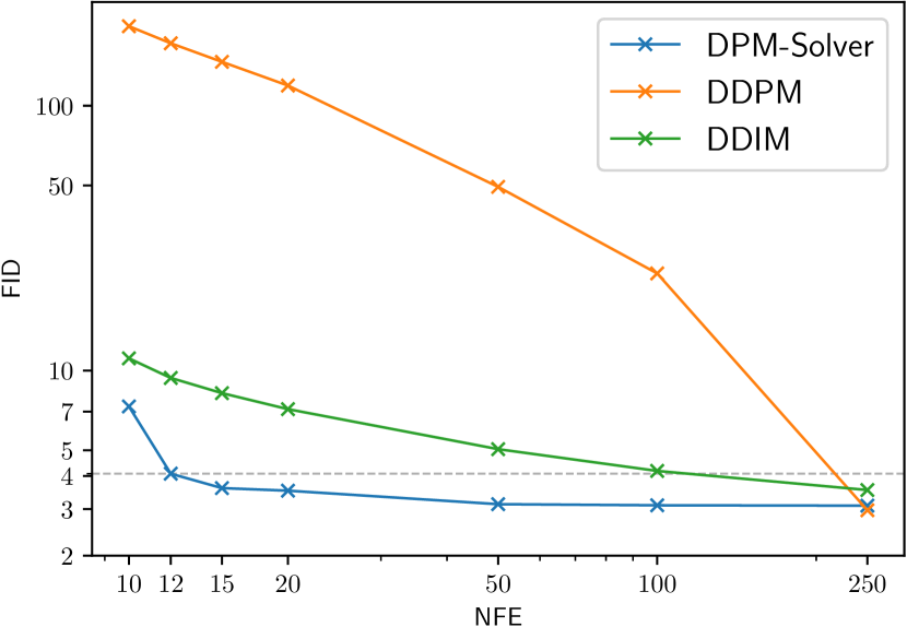
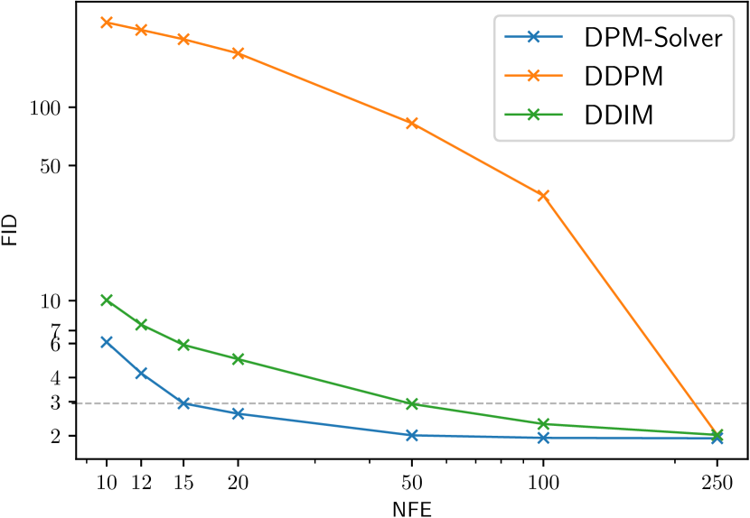
Based on our formulation of solutions, we propose DPM-Solver, a fast dedicated solver for diffusion ODEs by approximating the above integral. Specifically, we propose first-order, second-order and third-order versions of DPM-Solver with convergence order guarantees. We further propose an adaptive step size schedule for DPM-Solver. In general, DPM-Solver is applicable to both continuous-time and discrete-time DPMs, and also conditional sampling with classifier guidance [4]. Fig. 1 demonstrates the speedup performance of a Denoising Diffusion Implicit Models (DDIM) [19] baseline and DPM-Solver, which shows that DPM-Solver can generate high-quality samples with as few as 10 function evaluations and is much faster than DDIM on the ImageNet 256x256 dataset [26]. Our additional experimental results show that DPM-Solver can greatly improve the sampling speed of both discrete-time and continuous-time DPMs, and it can achieve excellent sample quality in around 10 function evaluations, which is much faster than all previous training-free samplers of DPMs.


2 Diffusion Probabilistic Models
We review diffusion probabilistic models and their associated differential equations in this section.
2.1 Forward Process and Diffusion SDEs
Assume that we have a -dimensional random variable with an unknown distribution . Diffusion Probabilistic Models (DPMs) [1, 2, 3, 10] define a forward process with starting with , such that for any , the distribution of conditioned on satisfies
| (2.1) |
where are differentiable functions of with bounded derivatives, and we denote them as for simplicity. The choice for and is referred to as the noise schedule of a DPM. Let denote the marginal distribution of , DPMs choose noise schedules to ensure that for some , and the signal-to-noise-ratio (SNR) is strictly decreasing w.r.t. [10]. Moreover, Kingma et al. [10] prove that the following stochastic differential equation (SDE) has the same transition distribution as in Eq. (2.1) for any :
| (2.2) |
where is the standard Wiener process, and
| (2.3) |
Under some regularity conditions, Song et al. [3] show that the forward process in Eq. (2.2) has an equivalent reverse process from time to , starting with the marginal distribution :
| (2.4) |
where is a standard Wiener process in the reverse time. The only unknown term in Eq. (2.4) is the score function at each time . In practice, DPMs use a neural network parameterized by to estimate the scaled score function: . The parameter is optimized by minimizing the following objective [2, 3]:
where is a weighting function, , , and is a constant independent of . As can also be regarded as predicting the Gaussian noise added to , it is usually called the noise prediction model. Since the ground truth of is , DPMs replace the score function in Eq. (2.4) by and define a parameterized reverse process (diffusion SDE) from time to , starting with :
| (2.5) |
Samples can be generated from DPMs by solving the diffusion SDE in Eq. (2.5) with numerical solvers, which discretize the SDE from to . Song et al. [3] proved that the traditional ancestral sampling method for DPMs [2] can be viewed as a first-order SDE solver for Eq. (2.5). However, these first-order methods usually need hundreds of or thousands of function evaluations to converge [3], leading to extremely slow sampling speed.
2.2 Diffusion (Probability Flow) ODEs
When discretizing SDEs, the step size is limited by the randomness of the Wiener process [27, Chap. 11]. A large step size (small number of steps) often causes non-convergence, especially in high dimensional spaces. For faster sampling, one can consider the associated probability flow ODE [3], which has the same marginal distribution at each time as that of the SDE. Specifically, for DPMs, Song et al. [3] proved that the probability flow ODE of Eq. (2.4) is
| (2.6) |
where the marginal distribution of is also . By replacing the score function with the noise prediction model, Song et al. [3] defined the following parameterized ODE (diffusion ODE):
| (2.7) |
Samples can be drawn by solving the ODE from to . Comparing with SDEs, ODEs can be solved with larger step sizes as they have no randomness. Furthermore, we can take advantage of efficient numerical ODE solvers to accelerate the sampling. Song et al. [3] used the RK45 ODE solver [28] for the diffusion ODEs, which generates samples in 60 function evaluations to reach comparable quality with a 1000-step SDE solver for Eq. (2.5) on the CIFAR-10 dataset [29]. However, existing general-purpose ODE solvers still cannot generate satisfactory samples in the few-step ( 10 steps) sampling regime. To the best of our knowledge, there is still a lack of training-free samplers for DPMs in the few-step sampling regime, and the sampling speed of DPMs is still a critical issue.
3 Customized Fast Solvers for Diffusion ODEs
As highlighted in Sec. 2.2, discretizing SDEs is generally difficult in high dimensions [27, Chap. 11] and it is hard to converge within few steps. In contrast, ODEs are easier to solve, yielding a potential for fast samplers. However, as mentioned in Sec. 2.2, the general black-box ODE solver used in previous work [3] empirically fails to converge in few steps. This motivates us to design a dedicated solver for diffusion ODEs to enable fast and high-quality few-step sampling. We start with a detailed investigation of the specific structure of diffusion ODEs.
3.1 Simplified Formulation of Exact Solutions of Diffusion ODEs
The key insight of this work is that given an initial value at time , the solution at each time of diffusion ODEs in Eq. (2.7) can be simplified into a very special exact formulation which can be efficiently approximated.
Our first key observation is that a part of the solution can be exactly computed by considering the particular structure of diffusion ODEs. The r.h.s. of diffusion ODEs in Eq. (2.7) consists of two parts: the part is a linear function of , and the other part is generally a nonlinear function of because of the neural network . This type of ODE is referred to as semi-linear ODE. The black-box ODE solvers adopted by previous work [3] are ignorant of this semi-linear structure as they take the whole in Eq. (2.7) as the input, which causes discretization errors of both the linear and nonlinear term. We note that for semi-linear ODEs, the solution at time can be exactly formulated by the “variation of constants” formula [30]:
| (3.1) |
This formulation decouples the linear part and the nonlinear part. In contrast to black-box ODE solvers, the linear part is now exactly computed, which eliminates the approximation error of the linear term. However, the integral of the nonlinear part is still complicated because it couples the coefficients about the noise schedule (i.e., ) and the complex neural network , which is still hard to approximate.
Our second key observation is that the integral of the nonlinear part can be greatly simplified by introducing a special variable. Let (one half of the log-SNR), then is a strictly decreasing function of (due to the definition of DPMs as discussed in Sec. 2.1). We can rewrite in Eq. (2.3) as
| (3.2) |
Combining with in Eq. (2.3), we can rewrite Eq. (3.1) as
| (3.3) |
As is a strictly decreasing function of , it has an inverse function satisfying . We further change the subscripts of and from to and denote , . Rewrite Eq. (3.3) by “change-of-variable” for , then we have:
Proposition 3.1 (Exact solution of diffusion ODEs).
Given an initial value at time , the solution at time of diffusion ODEs in Eq. (2.7) is:
| (3.4) |
We call the integral the exponentially weighted integral of , which is very special and highly related to the exponential integrators in the literature of ODE solvers [25]. To the best of our knowledge, such formulation has not been revealed in prior work of diffusion models.
Eq. (3.4) provides a new perspective for approximating the solutions of diffusion ODEs. Specifically, given at time , According to Eq. (3.4), approximating the solution at time is equivalent to directly approximating the exponentially weighted integral of from to , which avoids the error of the linear terms and is well-studied in the literature of exponential integrators [25, 31]. Based on this insight, we propose fast solvers for diffusion ODEs, as detailed in the following sections.
3.2 High-Order Solvers for Diffusion ODEs
In this section, we propose high-order solvers for diffusion ODEs with convergence order guarantee by leveraging our proposed solution formulation Eq. (3.4). The proposed solvers and analysis are highly motivated by the methods of exponential integrators [25, 31] in the ODE literature.
Specifically, given an initial value at time and time steps decreasing from to . Let be the initial value. The proposed solvers use steps to iteratively compute a sequence to approximate the true solutions at time steps . In particular, the last iterate approximates the true solution at time .
In order to reduce the approximation error between and the true solution at time , we need to reduce the approximation error for each at every step [30]. Starting with the previous value at time , according to Eq. (3.4), the exact solution at time is given by
| (3.5) |
Therefore, to compute the value for approximating , we need to approximate the exponentially weighted integral of from to . Denote , and as the -th order total derivative of w.r.t. . For , the -th order Taylor expansion of w.r.t. at is
Substituting the above Taylor expansion into Eq. (3.5) yields
| (3.6) |
where the integral can be analytically computed by repeatedly applying times of integration-by-parts (see Appendix B.2). Therefore, to approximate , we only need to approximate the -th order total derivatives for , which is a well-studied problem in the ODE literature [31, 32]. By dropping the error term and approximating the first -th total derivatives with the “stiff order conditions” [31, 32], we can derive -th-order ODE solvers for diffusion ODEs. We name such solvers as DPM-Solver overall, and DPM-Solver- for a specific order . Here we take for demonstration. In this case, Eq. (3.6) becomes
By dropping the high-order error term , we can obtain an approximation for . As here, we call this solver DPM-Solver-1, and the detailed algorithm is as following.
DPM-Solver-1. Given an initial value and time steps decreasing from to . Starting with , the sequence is computed iteratively as follows:
| (3.7) |
For , approximating the first terms of the Taylor expansion needs additional intermediate points between and [31]. The derivation is more technical so we defer it to Appendix B. Below we propose algorithms for and name them as DPM-Solver-2 and DPM-Solver-3, respectively.
Here, is the inverse function of , which has an analytical formulation for the practical noise schedule used in [2, 16], as shown in Appendix D. The chosen intermediate points are (, ) for DPM-Solver-2 and and for DPM-Solver-3. As shown in the algorithm, DPM-Solver- requires function evaluations per step for . Despite the more expensive steps, higher-order solvers () are usually more efficient since they require much fewer steps to converge, due to their higher convergence order. We show that DPM-Solver- is -th-order solver, as stated in the following theorem. The proof is in Appendix B.
Theorem 3.2 (DPM-Solver- as a -th-order solver).
Assume follows the regularity conditions detailed in Appendix B.1, then for , DPM-Solver- is a -th order solver for diffusion ODEs, i.e., for the sequence computed by DPM-Solver-, the approximation error at time satisfies , where .
3.3 Step Size Schedule
The proposed solvers in Sec. 3.2 need to specify the time steps in advance. We propose two choices of the time step schedule. One choice is handcrafted, which is to uniformly split the interval , ], i.e. , . Note that this is different from previous work [2, 3] which chooses uniform steps for . Empirically, DPM-Solver with uniform time steps can already generate quite good samples in few steps, where results are listed in Appendix E. As the other choice, we propose an adaptive step size algorithm, which dynamically adjusts the step size by combining different orders of DPM-Solver. The adaptive algorithm is inspired by [20] and we defer its implementation details to Appendix C.
For few-step sampling, we need to use up all the number of function evaluations (NFE). When the NFE is not divisible by , we firstly apply DPM-Solver-3 as much as possible, and then add a single step of DPM-Solver-1 or DPM-Solver-2 (dependent on the reminder of divided by ), as detailed in Appendix D. In the subsequent experiments, we use such combination of solvers with the uniform step size schedule for NFE , and otherwise the adaptive step size schedule.
3.4 Sampling from Discrete-Time DPMs
Discrete-time DPMs [2] train the noise prediction model at fixed time steps , and the noise prediction model is parameterized by for , where each is corresponding to the value at time . We can transform the discrete-time noise prediction model to the continuous version by letting , for all . Note that the input time of may not be integers, but we find that the noise prediction model can still work well, and we hypothesize that it is because of the smooth time embeddings (e.g., position embeddings [2]). By such reparameterization, the noise prediction model can adopt the continuous-time steps as input, and thus we can also use DPM-Solver for fast sampling.
4 Comparison with Existing Fast Sampling Methods
Here, we discuss the relationship and highlight the difference between DPM-Solver and existing ODE-based fast sampling methods for DPMs. We further briefly discuss the advantage of training-free samplers over those training-based ones.
4.1 DDIM as DPM-Solver-1
Denoising Diffusion Implicit Models (DDIM) [19] design a deterministic method for fast sampling from DPMs. For two adjacent time steps and , assume that we have a solution at time , then a single step of DDIM from time to time is
| (4.1) |
Although motivated by entirely different perspectives, we show that the updates of DPM-Solver-1 and Denoising Diffusion Implicit Models (DDIM) [19] are identical. By the definition of , we have and . Plugging these and to Eq. (4.1) results in exactly a step of DPM-Solver-1 in Eq. (3.7). However, the semi-linear ODE formulation of DPM-Solver allows for principled generalization to higher-order solvers and convergence order analysis.
Recent work [13] also show that DDIM is a first-order discretization of diffusion ODEs by differentiating both sides of Eq. (4.1). However, they cannot explain the difference between DDIM and the first-order Euler discretization of diffusion ODEs. In contrast, by showing that DDIM is a special case of DPM-Solver, we reveal that DDIM makes full use of the semi-linearity of diffusion ODEs, which explains its superiority over traditional Euler methods.
4.2 Comparison with Traditional Runge-Kutta Methods
One can obtain a high-order solver by directly applying traditional explicit Runge-Kutta (RK) methods to the diffusion ODE in Eq. (2.7). Specifically, RK methods write the solution of Eq. (2.7) in the following integral form:
| (4.2) |
and use some intermediate time steps between and combine the evaluations of at these time steps to approximate the whole integral. The approximation error of explicit RK methods depends on , which consists of the error corresponding to both the linear term and the nonlinear noise prediction model . However, the error of the linear term may increase exponentially because the exact solution of the linear term has an exponential coefficient (as shown in Eq. (3.1)). There are many empirical evidence [25, 31] showing that directly using explicit RK methods for semi-linear ODEs may suffer from unstable numerical issues for large step size. We also demonstrate the empirical difference of the proposed DPM-Solver and the traditional explicit RK methods in Sec. 5.1, which shows that DPM-Solver have smaller discretization errors than the RK methods with the same order.
4.3 Training-based Fast Sampling Methods for DPMs
Samplers that need extra training or optimization include knowledge distillation [13, 14], learning the noise level or variance [15, 16, 33], and learning the noise schedule or sample trajectory [17, 18]. Although the progressive distillation method [13] can obtain a fast sampler within 4 steps, it needs further training costs and loses part of the information in the original DPM (e.g., after distillation, the noise prediction model cannot predict the noise (score function) at every time step between ). In contrast, training-free samplers can keep all the information of the original model, and thereby can be directly extended to the conditional sampling by combining the original model and an external classifier [4] (e.g. see Appendix D for the conditional sampling with classifier guidance).
Beyond directly designing fast samplers for DPMs, several works also propose novel types of DPMs which supports faster sampling. For instance, defining a low-dimensional latent variable for DPMs [34]; designing special diffusion processes with bounded score functions [35]; combining GANs with the reverse process of DPMs [36]. The proposed DPM-Solver may also be suitable for accelerating the sampling of these DPMs, and we leave them for future work.
| Sampling method NFE | 12 | 18 | 24 | 30 | 36 | 42 | 48 |
|---|---|---|---|---|---|---|---|
| RK2 () | 16.40 | 7.25 | 3.90 | 3.63 | 3.58 | 3.59 | 3.54 |
| RK2 () | 107.81 | 42.04 | 17.71 | 7.65 | 4.62 | 3.58 | 3.17 |
| DPM-Solver-2 | 5.28 | 3.43 | 3.02 | 2.85 | 2.78 | 2.72 | 2.69 |
| RK3 () | 48.75 | 21.86 | 10.90 | 6.96 | 5.22 | 4.56 | 4.12 |
| RK3 () | 34.29 | 4.90 | 3.50 | 3.03 | 2.85 | 2.74 | 2.69 |
| DPM-Solver-3 | 6.03 | 2.90 | 2.75 | 2.70 | 2.67 | 2.65 | 2.65 |
5 Experiments
In this section, we show that as a training-free sampler, DPM-Solver can greatly speedup the sampling of existing pre-trained DPMs, including both continuous-time and discrete-time ones, with both linear noise schedule [2, 19] and cosine noise schedule [16]. We vary different number of function evaluations (NFE) which is the number of calls to the noise prediction model , and compare the sample quality between DPM-Solver and other methods. For each experiment, We draw 50K samples and use the widely adopted FID score [37] to evaluate the sample quality, where lower FID usually implies better sample quality.
Unless explicitly mentioned, we always use the solver combination with the uniform step size schedule in Sec. 3.3 if the NFE budget is less than 20, and otherwise the DPM-Solver-3 with the adaptive step size schedule in Sec. 3.3. We refer to Appendix D for other implementation details of DPM-Solver and Appendix E for detailed settings.
5.1 Comparison with Continuous-Time Sampling Methods
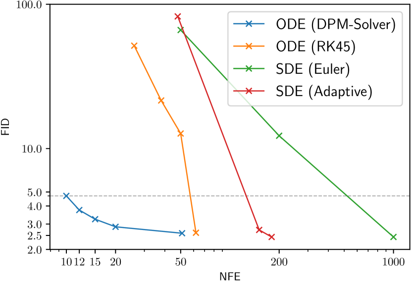
We firstly compare DPM-Solver with other continuous-time sampling methods for DPMs. The compared methods include the Euler-Maruyama discretization for diffusion SDEs [3], the adaptive step size solver for diffusion SDEs [20] and the RK methods for diffusion ODEs [3, 28] in Eq. (2.7). We compare these methods for sampling from a pre-trained continuous-time “VP deep” model [3] on the CIFAR-10 dataset [29] with the linear noise schedule.
Fig. 2(a) shows the efficiency of compared solvers. We use uniform time steps with 50, 200, 1000 NFE for the diffusion SDE with Euler discretization, and vary the tolerance hyperparameter [3, 20] for the adaptive step size SDE solver [20] and RK45 ODE solver [28] to control the NFE. DPM-Solver can generate good sample quality within around 10 NFE, while other solvers have large discretization error even in 50 NFE, which shows that DPM-Solver can achieve 5 speedup of the previous best solver. In particular, we achieve 4.70 FID with 10 NFE, 3.75 FID with 12 NFE, 3.24 FID with 15 NFE, and 2.87 FID with 20 NFE, which is the fastest sampler on CIFAR-10.
As an ablation study, we also compare the second-order and third-order DPM-Solver and RK methods, as shown in Table 1. We compare RK methods for diffusion ODEs w.r.t. both time in Eq. (2.7) and half-log-SNR by applying change-of-variable (see detailed formulations in Appendix E.1). The results show that given the same NFE, the sample quality of DPM-Solver is consistently better than RK methods with the same order. The superior efficiency of DPM-Solver is particularly evident in the few-step regime under 15 NFE, where RK methods have rather large discretization errors. This is mainly because DPM-Solver analytically computes the linear term, avoiding the corresponding discretization error. Besides, the higher order DPM-Solver-3 converges faster than DPM-Solver-2, which matches the order analysis in Theorem 3.2.
5.2 Comparison with Discrete-Time Sampling Methods
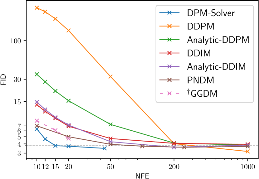
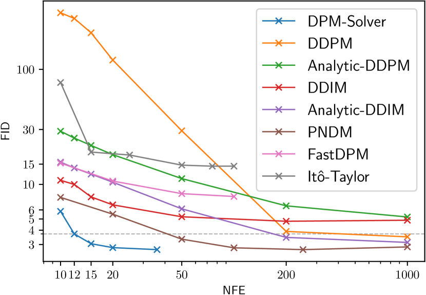
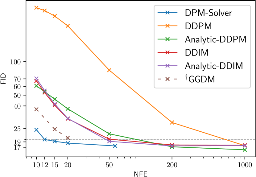
We use the method in Sec. 3.4 for using DPM-Solver in discrete-time DPMs, and then compare DPM-Solver with other discrete-time training-free samplers, including DDPM [2], DDIM [19], Analytic-DDPM [21], Analytic-DDIM [21], PNDM [22], FastDPM [38] and Itô-Taylor [24]. We also compare with GGDM [18], which uses the same pre-trained model but needs further training for the sampling trajectory. We compare the sample quality by varying NFE from 10 to 1000.
Specifically, we use the discrete-time model trained by in [2] on the CIFAR-10 dataset with linear noise schedule; the discrete-time model in [19] on CelebA 64x64 [39] with linear noise schedule; the discrete-time model trained by in [16] on ImageNet 64x64 [26] with cosine noise schedule; the discrete-time model with classifier guidance in [4] on ImageNet 128x128 [26] with linear noise schedule; the discrete-time model in [4] on LSUN bedroom 256x256 [40] with linear noise schedule. For the models trained on ImageNet, we only use their “mean” model and omit the “variance” model. As shown in Fig. 2, on all datasets, DPM-Solver can obtain reasonable samples within 12 steps (FID 4.65 on CIFAR-10, FID 3.71 on CelebA 64x64 and FID 19.97 on ImageNet 64x64, FID 4.08 on ImageNet 128x128), which is faster than the previous fastest training-free sampler. DPM-Solver even outperforms GGDM, which requires additional training.
6 Conclusions
We tackle the problem of fast and training-free sampling from DPMs. We propose DPM-Solver, a fast dedicated training-free solver of diffusion ODEs for fast sampling of DPMs in around 10 steps of function evaluations. DPM-Solver leverages the semi-linearity of diffusion ODEs and it directly approximates a simplified formulation of exact solutions of diffusion ODEs, which consists of an exponentially weighted integral of the noise prediction model. Inspired by numerical methods for exponential integrators, we propose first-order, second-order and third-order DPM-Solver to approximate the exponentially weighted integral of noise prediction models with theoretical convergence guarantee. We propose both handcrafted and adaptive step size schedule, and apply DPM-Solver for both continuous-time and discrete-time DPMs. Our experimental results show that DPM-Solver can generate high-quality samples in around 10 function evaluations on various datasets, and it can achieve speedup compared with previous state-of-the-art training-free samplers.
Limitations and broader impact Despite the promising speedup performance, DPM-Solver is designed for fast sampling, which may be not suitable for accelerating the likelihood evaluations of DPMs. Besides, compared to the commonly-used GANs, diffusion models with DPM-Solver are still not fast enough for real-time applications. In addition, like other deep generative models, DPMs may be used to generate adverse fake contents, and the proposed solver may further amplify the potential undesirable influence of deep generative models for malicious applications.
Acknowledgements
This work was supported by National Key Research and Development Project of China (No. 2021ZD0110502); NSF of China Projects (Nos. 62061136001, 61620106010, 62076145, U19B2034, U1811461, U19A2081, 6197222, 62106120); Beijing NSF Project (No. JQ19016); Beijing Outstanding Young Scientist Program NO. BJJWZYJH012019100020098; a grant from Tsinghua Institute for Guo Qiang; the NVIDIA NVAIL Program with GPU/DGX Acceleration; the High Performance Computing Center, Tsinghua University; the Fundamental Research Funds for the Central Universities, and the Research Funds of Renmin University of China (22XNKJ13). J.Z is also supported by the XPlorer Prize.
References
- Sohl-Dickstein et al. [2015] J. Sohl-Dickstein, E. Weiss, N. Maheswaranathan, and S. Ganguli, “Deep unsupervised learning using nonequilibrium thermodynamics,” in International Conference on Machine Learning. PMLR, 2015, pp. 2256–2265.
- Ho et al. [2020] J. Ho, A. Jain, and P. Abbeel, “Denoising diffusion probabilistic models,” in Advances in Neural Information Processing Systems, vol. 33, 2020, pp. 6840–6851.
- Song et al. [2021a] Y. Song, J. Sohl-Dickstein, D. P. Kingma, A. Kumar, S. Ermon, and B. Poole, “Score-based generative modeling through stochastic differential equations,” in International Conference on Learning Representations, 2021.
- Dhariwal and Nichol [2021] P. Dhariwal and A. Q. Nichol, “Diffusion models beat GANs on image synthesis,” in Advances in Neural Information Processing Systems, vol. 34, 2021, pp. 8780–8794.
- Meng et al. [2022] C. Meng, Y. Song, J. Song, J. Wu, J.-Y. Zhu, and S. Ermon, “SDEdit: Image synthesis and editing with stochastic differential equations,” in International Conference on Learning Representations, 2022.
- Ho et al. [2022] J. Ho, T. Salimans, A. Gritsenko, W. Chan, M. Norouzi, and D. J. Fleet, “Video diffusion models,” arXiv preprint arXiv:2204.03458, 2022.
- Ramesh et al. [2022] A. Ramesh, P. Dhariwal, A. Nichol, C. Chu, and M. Chen, “Hierarchical text-conditional image generation with CLIP latents,” arXiv preprint arXiv:2204.06125, 2022.
- Chen et al. [2021a] N. Chen, Y. Zhang, H. Zen, R. J. Weiss, M. Norouzi, and W. Chan, “Wavegrad: Estimating gradients for waveform generation,” in International Conference on Learning Representations, 2021.
- Chen et al. [2021b] N. Chen, Y. Zhang, H. Zen, R. J. Weiss, M. Norouzi, N. Dehak, and W. Chan, “Wavegrad 2: Iterative refinement for text-to-speech synthesis,” in International Speech Communication Association, 2021, pp. 3765–3769.
- Kingma et al. [2021] D. P. Kingma, T. Salimans, B. Poole, and J. Ho, “Variational diffusion models,” in Advances in Neural Information Processing Systems, 2021.
- Goodfellow et al. [2014] I. J. Goodfellow, J. Pouget-Abadie, M. Mirza, B. Xu, D. Warde-Farley, S. Ozair, A. C. Courville, and Y. Bengio, “Generative adversarial nets,” in Advances in Neural Information Processing Systems, vol. 27, 2014, pp. 2672–2680.
- Kingma and Welling [2014] D. P. Kingma and M. Welling, “Auto-encoding variational bayes,” in International Conference on Learning Representations, 2014.
- Salimans and Ho [2022] T. Salimans and J. Ho, “Progressive distillation for fast sampling of diffusion models,” in International Conference on Learning Representations, 2022.
- Luhman and Luhman [2021] E. Luhman and T. Luhman, “Knowledge distillation in iterative generative models for improved sampling speed,” arXiv preprint arXiv:2101.02388, 2021.
- San-Roman et al. [2021] R. San-Roman, E. Nachmani, and L. Wolf, “Noise estimation for generative diffusion models,” arXiv preprint arXiv:2104.02600, 2021.
- Nichol and Dhariwal [2021] A. Q. Nichol and P. Dhariwal, “Improved denoising diffusion probabilistic models,” in International Conference on Machine Learning. PMLR, 2021, pp. 8162–8171.
- Lam et al. [2021] M. W. Lam, J. Wang, R. Huang, D. Su, and D. Yu, “Bilateral denoising diffusion models,” arXiv preprint arXiv:2108.11514, 2021.
- Watson et al. [2022] D. Watson, W. Chan, J. Ho, and M. Norouzi, “Learning fast samplers for diffusion models by differentiating through sample quality,” in International Conference on Learning Representations, 2022.
- Song et al. [2021b] J. Song, C. Meng, and S. Ermon, “Denoising diffusion implicit models,” in International Conference on Learning Representations, 2021.
- Jolicoeur-Martineau et al. [2021] A. Jolicoeur-Martineau, K. Li, R. Piché-Taillefer, T. Kachman, and I. Mitliagkas, “Gotta go fast when generating data with score-based models,” arXiv preprint arXiv:2105.14080, 2021.
- Bao et al. [2022a] F. Bao, C. Li, J. Zhu, and B. Zhang, “Analytic-DPM: An analytic estimate of the optimal reverse variance in diffusion probabilistic models,” in International Conference on Learning Representations, 2022.
- Liu et al. [2022] L. Liu, Y. Ren, Z. Lin, and Z. Zhao, “Pseudo numerical methods for diffusion models on manifolds,” in International Conference on Learning Representations, 2022.
- Popov et al. [2022] V. Popov, I. Vovk, V. Gogoryan, T. Sadekova, M. Kudinov, and J. Wei, “Diffusion-based voice conversion with fast maximum likelihood sampling scheme,” in International Conference on Learning Representations, 2022.
- Tachibana et al. [2021] H. Tachibana, M. Go, M. Inahara, Y. Katayama, and Y. Watanabe, “Itô-Taylor sampling scheme for denoising diffusion probabilistic models using ideal derivatives,” arXiv preprint arXiv:2112.13339, 2021.
- Hochbruck and Ostermann [2010] M. Hochbruck and A. Ostermann, “Exponential integrators,” Acta Numerica, vol. 19, pp. 209–286, 2010.
- Deng et al. [2009] J. Deng, W. Dong, R. Socher, L. Li, K. Li, and L. Fei-Fei, “ImageNet: A large-scale hierarchical image database,” in 2009 IEEE Conference on Computer Vision and Pattern Recognition. IEEE, 2009, pp. 248–255.
- Kloeden and Platen [1992] P. E. Kloeden and E. Platen, Numerical Solution of Stochastic Differential Equations. Springer, 1992.
- Dormand and Prince [1980] J. R. Dormand and P. J. Prince, “A family of embedded Runge-Kutta formulae,” Journal of computational and applied mathematics, vol. 6, no. 1, pp. 19–26, 1980.
- Krizhevsky [2009] A. Krizhevsky, “Learning multiple layers of features from tiny images,” Tech. Rep., 2009.
- Atkinson et al. [2011] K. Atkinson, W. Han, and D. E. Stewart, Numerical solution of ordinary differential equations. John Wiley & Sons, 2011, vol. 108.
- Hochbruck and Ostermann [2005] M. Hochbruck and A. Ostermann, “Explicit exponential Runge-Kutta methods for semilinear parabolic problems,” SIAM Journal on Numerical Analysis, vol. 43, no. 3, pp. 1069–1090, 2005.
- Luan [2021] V. T. Luan, “Efficient exponential Runge-Kutta methods of high order: Construction and implementation,” BIT Numerical Mathematics, vol. 61, no. 2, pp. 535–560, 2021.
- Bao et al. [2022b] F. Bao, C. Li, J. Sun, J. Zhu, and B. Zhang, “Estimating the optimal covariance with imperfect mean in diffusion probabilistic models,” arXiv preprint arXiv:2206.07309, 2022.
- Vahdat et al. [2021] A. Vahdat, K. Kreis, and J. Kautz, “Score-based generative modeling in latent space,” in Advances in Neural Information Processing Systems, vol. 34, 2021, pp. 11 287–11 302.
- Dockhorn et al. [2022] T. Dockhorn, A. Vahdat, and K. Kreis, “Score-based generative modeling with critically-damped Langevin diffusion,” in International Conference on Learning Representations, 2022.
- Xiao et al. [2022] Z. Xiao, K. Kreis, and A. Vahdat, “Tackling the generative learning trilemma with denoising diffusion GANs,” in International Conference on Learning Representations, 2022.
- Heusel et al. [2017] M. Heusel, H. Ramsauer, T. Unterthiner, B. Nessler, and S. Hochreiter, “GANs trained by a two time-scale update rule converge to a local Nash equilibrium,” in Advances in Neural Information Processing Systems, I. Guyon, U. von Luxburg, S. Bengio, H. M. Wallach, R. Fergus, S. V. N. Vishwanathan, and R. Garnett, Eds., vol. 30, 2017, pp. 6626–6637.
- Kong and Ping [2021] Z. Kong and W. Ping, “On fast sampling of diffusion probabilistic models,” arXiv preprint arXiv:2106.00132, 2021.
- Liu et al. [2015] Z. Liu, P. Luo, X. Wang, and X. Tang, “Deep learning face attributes in the wild,” in Proceedings of the IEEE International Conference on Computer Vision, 2015, pp. 3730–3738.
- Yu et al. [2015] F. Yu, A. Seff, Y. Zhang, S. Song, T. Funkhouser, and J. Xiao, “LSUN: Construction of a large-scale image dataset using deep learning with humans in the loop,” arXiv preprint arXiv:1506.03365, 2015.
- Song et al. [2021c] Y. Song, C. Durkan, I. Murray, and S. Ermon, “Maximum likelihood training of score-based diffusion models,” in Advances in Neural Information Processing Systems, vol. 34, 2021, pp. 1415–1428.
- Yang et al. [2021] K. Yang, J. Yau, L. Fei-Fei, J. Deng, and O. Russakovsky, “A study of face obfuscation in ImageNet,” arXiv preprint arXiv:2103.06191, 2021.
Checklist
-
1.
For all authors…
-
(a)
Do the main claims made in the abstract and introduction accurately reflect the paper’s contributions and scope? [Yes]
-
(b)
Did you describe the limitations of your work? [Yes] See section 6.
-
(c)
Did you discuss any potential negative societal impacts of your work? [Yes] See section 6.
-
(d)
Have you read the ethics review guidelines and ensured that your paper conforms to them? [Yes]
-
(a)
- 2.
-
3.
If you ran experiments…
-
(a)
Did you include the code, data, and instructions needed to reproduce the main experimental results (either in the supplemental material or as a URL)? [Yes] Code is attached in the supplemental materials, with the appendix.
-
(b)
Did you specify all the training details (e.g., data splits, hyperparameters, how they were chosen)? [Yes] Our method is training-free. But we also report the hyperparameters for evaluations used in our proposed solver.
-
(c)
Did you report error bars (e.g., with respect to the random seed after running experiments multiple times)? [No] We observe that the standard deviation of the FID evaluations of DPM-Solver are rather small (mainly less than 0.01) because the FID is already averaged over 50K samples, following existing work [18, 20, 21]. The small standard deviation does not change the conclusion.
-
(d)
Did you include the total amount of compute and the type of resources used (e.g., type of GPUs, internal cluster, or cloud provider)? [Yes] The GPU type and amount is detailed in Appendix E.
-
(a)
-
4.
If you are using existing assets (e.g., code, data, models) or curating/releasing new assets…
-
(a)
If your work uses existing assets, did you cite the creators? [Yes]
-
(b)
Did you mention the license of the assets? [Yes] See Appendix E
-
(c)
Did you include any new assets either in the supplemental material or as a URL? [Yes] We include our code in the supplemental materials.
-
(d)
Did you discuss whether and how consent was obtained from people whose data you’re using/curating? [No] All of the datasets used in the experiments are publicly available.
-
(e)
Did you discuss whether the data you are using/curating contains personally identifiable information or offensive content? [Yes] We mentioned the human privacy issues of the ImageNet dataset in Appendix E.
-
(a)
-
5.
If you used crowdsourcing or conducted research with human subjects…
-
(a)
Did you include the full text of instructions given to participants and screenshots, if applicable? [N/A]
-
(b)
Did you describe any potential participant risks, with links to Institutional Review Board (IRB) approvals, if applicable? [N/A]
-
(c)
Did you include the estimated hourly wage paid to participants and the total amount spent on participant compensation? [N/A]
-
(a)
Appendix A Sampling with Invariance to the Noise Schedule
| Method | Invariance Formulation |
|---|---|
| Maximum likelihood training | |
| Sampling by diffusion ODEs |
In this section, we discuss more about the exact solution in Proposition 3.1 and give some insights about the formulation. Below we firstly restate the proposition w.r.t. (i.e. the half-logSNR).
Proposition 3.1 (Exact solution of diffusion ODEs).
Given an initial value at time with the corresponding half-logSNR , the solution at time of diffusion ODEs in Eq. (2.7) with the corresponding half-logSNR is:
| (A.1) |
In the following subsections, we will show that such formulation decouples the model from the specific noise schedule, and thus is invariant to the noise schedule. Moreover, such change-of-variable for in Proposition 3.1 is highly related to the maximum likelihood training of diffusion models [10, 41]. We show that both the maximum likelihood training and the sampling of diffusion models have invariance formulations that are independent of the noise schedule.
A.1 Decoupling the Sampling Solution from the Noise Schedule
In this section, we show that Proposition 3.1 can decouples the exact solutions of the diffusion ODEs from the specific noise schedules (i.e. choice of the functions and ). Namely, given a starting point , a ending point , an initial value at and a noise prediction model , the solution of is invariant of the noise schedule between and .
We firstly consider the VP type diffusion models, which is equivalent to the original DDPM [2, 3]. For VP type diffusion models, we always have , so defining the noise schedule is equivalent to defining the function (For example, DDPM [2] uses a noise schedule such that is a linear function of , and i-DDPM [16] uses a noise schedule such that is a cosine function of ). As , we have and . Thus, we can directly compute the and for a given . Denote , we have
| (A.2) |
We should notice that the integrand is a function of , so its integral from to is only dependent on the starting point , the ending point and the function , which is independent of the intermediate values. As other coefficients ( and ) are also only dependent on the starting point and the ending point , we can conclude that is invariant of the specific choice of the noise schedules. Intuitively, this is because we converts the original integral of time in Eq. (3.1) to the integral of , and the functions and are converted to an analytical formulation , which is invariant to the specific choices of and . Finally, for other types of diffusion models (such as the VE type and the subVP type), they are all equivalent to the VP type by equivalently rescaling the noise prediction models, as proved in [10]. Therefore, the solutions of these types also have such property.
In summary, Proposition 3.1 decouples the solution of diffusion ODEs from the noise schedules, which gives us an opportunity to design tailor-made samplers for DPMs. In fact, as shown in Sec. 3.2, the only approximation of the proposed DPM-Solver is about the Taylor expansion of the neural network w.r.t. , and DPM-Solver analytically computes other coefficients (which are corresponding to the specific noise schedules). Intuitively, DPM-Solver keeps the known information as much as possible, and only approximates the intractable integral of the neural network, so it can generate comparable samples within much fewer steps.
A.2 Choosing Time Steps for is Invariant to the Noise Schedule
As mentioned in Appendix A.1, the formulation of Proposition 3.1 decouples the sampling solution from the noise schedule. The solution depends on the starting point and the ending point , and is invariant to the intermediate noise schedule. Similarly, the updating equations of the algorithm of DPM-Solver are also invariant to the intermediate noise schedule. Therefore, if we have chosen the time steps , then the solution of DPM-Solver is also determined and is invariant to the intermediate noise schedule.
A simple way for choosing time steps for is uniformly splitting , which is the setting in our experiments. However, we believe that there exists more precise ways for choosing the time steps, and we leave it for future work.
A.3 Relationship with the Maximum Likelihood Training of Diffusion Models
Interestingly, the maximum likelihood training of diffusion SDEs in continuous time also has such invariance property [10]. Below we briefly review the maximum likelihood training loss of diffusion SDEs, and then propose a new insight for understanding diffusion models.
Denote the data distribution as , the distribution of the forward process at each time as , the distribution of the reverse process at each time as with . In [3], it is proved that the KL-divergence between and can be bounded by a weighted score matching loss:
| (A.3) |
where and is a constant independent of . As shown in Sec. 3.1, we have
| (A.4) |
so by applying change-of-variable w.r.t. , we have
| (A.5) |
which is equivalent to the importance sampling trick in [41, Sec. 5.1] and the continuous-time diffusion loss in [10, Eq. (22)]. Compared to Proposition 3.1, we can find that the sampling and the maximum likelihood training of diffusion models can both be converted to an integral w.r.t. , such that the formulation is invariant to the specific noise schedules, and we summarize it in Table 2. Such invariance property for both training and sampling brings a new insight for understanding diffusion models. For instance, we can directly define the noise prediction model w.r.t. the (half-)logSNR instead of the time , then the training and sampling for diffusion models can be done without further choosing any ad-hoc noise schedules. Such finding may unify the different ways of the training and the inference of diffusion models, and we leave it for future study.
Appendix B Proof of Theorem 3.2
B.1 Assumptions
Throughout this section, we denote as the solution of the diffusion ODE Eq. (2.7) starting from . For DPM-Solver- we make the following assumptions:
Assumption B.1.
The total derivatives (as a function of ) exist and are continuous for .
Assumption B.2.
The function is Lipschitz w.r.t. to its first parameter .
Assumption B.3.
.
We note that the first assumption is required by Taylor’s theorem Eq. (3.6), and the second assumption is used to replace with so that the Taylor expansion w.r.t. is applicable. The last one is a technical assumption to exclude a significantly large step-size.
B.2 General Expansion of the Exponentially Weighted Integral
Firstly, we derive the Taylor expansion of the exponentially weighted integral. Let and then . Denote , and the -th order total derivative . For , the -th order Taylor expansion of w.r.t. is
| (B.1) |
To expand the exponential integrator, we further define [31]:
| (B.2) |
and it satisfies and a recurrence relation . By taking the Taylor expansion of , the exponential integrator can be rewritten as
| (B.3) |
So the solution of in Eq. (3.4) can be expanded as
| (B.4) |
Finally, we list the closed-forms of for :
| (B.5) | ||||
| (B.6) | ||||
| (B.7) |
B.3 Proof of Theorem 3.2 when
B.4 Proof of Theorem 3.2 when
We prove the discretization error of the general form of DPM-Solver-2 in Algorithm 4.
Proof.
First, we consider the following update for .
| (B.9a) | ||||
| (B.9b) | ||||
| (B.9c) | ||||
Note that the above update is the same as a single step of DPM-Solver-2 with and , except that is replaced with the exact solution . Once we have proven that , we can show that by a similar argument as in Appendix B.3, and therefore completes the proof.
In this remaining part we prove that .
Taking in Eq. (B.4), we obtain
| (B.10) |
From Eq. (B.1), we have
Note that by the Lipschitzness of w.r.t. (Assumption B.2),
where the last equation follows from a similar argument in the proof of . Since , the second term of the above display is .
As , and , we find
Then, the proof is completed by noticing that
∎
B.5 Proof of Theorem 3.2 when
Proof.
As in Appendix B.4, it suffices to show that the following update has error for and .
| (B.11a) | ||||
| (B.11b) | ||||
| (B.11c) | ||||
| (B.11d) | ||||
| (B.11e) | ||||
| (B.11f) | ||||
First, we prove that
| (B.12) |
Similar to the proof in Appendix B.4, since and , then
Let , then following the same line of arguments in the proof of Appendix B.4, it suffices to check that
which holds by applying Taylor expansion.
Using and , we find that
Comparing with the Taylor expansion in Eq. (B.4) with :
we need to check the following conditions:
The first two conditions are clear. The last condition follows from
Therefore, . ∎
B.6 Connections to Explicit Exponential Runge-Kutta (expRK) Methods
Assume we have an ODE with the following form:
where and is a non-linear function of . Given an initial value at time , for , the true solution at time is
The exponential Runge-Kutta methods [25, 31] use some intermediate points to approximate the integral . Our proposed DPM-Solver is inspired by the same technique for approximating the same integral with and . However, DPM-Solver is different from the expRK methods, because their linear term is different from our linear term . In summary, DPM-Solver is inspired by the same technique of expRK for deriving high-order approximations of the exponentially weighted integral, but the formulation of DPM-Solver is different from expRK, and DPM-Solver is customized for the specific formulation of diffusion ODEs.
Appendix C Algorithms of DPM-Solvers
We firstly list the detailed DPM-Solver-1, 2, 3 in Algorithms 3, 4, 5. Note that DPM-Solver-2 is the general case with , and we usually set for DPM-Solver-2, as in Sec. 3.
Then we list the adaptive step size algorithms, named as DPM-Solver-12 (combining 1 and 2; Algorithm 6) and DPM-Solver-23 (combining 2 and 3; Algorithm 7). We follow [20] to let the absolute tolerance for image data, which is for VP type DPMs. We can tune the relative tolerance to balance the accuracy and NFE, and we find that is good enough and can converge quickly.
In practice, the inputs of the adaptive step size solvers are batch data. We simply choose and as the maximum value of all the batch data. Besides, we implement the comparison by to avoid numerical issues.
Appendix D Implementation Details of DPM-Solver
D.1 End Time of Sampling
Theoretically, we need to solve diffusion ODEs from time to time to generate samples. Practically, the training and evaluation for the noise prediction model usually start from time to time to avoid numerical issues for near to , where is a hyperparameter [3].
In contrast to the sampling methods based on diffusion SDEs [2, 3], We don’t add the “denoising” trick at the final step at time (which is to set the noise variance to zero), and we just solve diffusion ODEs from to by DPM-Solver, since we find it performs well enough.
For discrete-time DPMs, we firstly convert the model to continuous time (see Appendix D.2), and then solver it from time to time .
D.2 Sampling from Discrete-Time DPMs
In this section, we discuss the more general case for discrete-time DPMs, in which we consider the 1000-step DPMs [2] and the 4000-step DPMs [16], and we also consider the end time for sampling.
Discrete-time DPMs [2] train the noise prediction model at fixed time steps . In practice, or , and the implementation of the 4000-step DPMs [16] converts the time steps of 4000-step DPMs to the range of 1000-step DPMs. Specifically, the noise prediction model is parameterized by for , where each is corresponding to the value at time . In practice, these discrete-time DPMs usually choose uniform time steps between , thus , for .
However, the discrete-time noise prediction model cannot predict the noise at time less than the smallest time . As the smallest time step and the corresponding discrete-time noise prediction model at time is , we need to “scale” the discrete time steps to the continuous time range . We propose two types of scaling as following.
Type-1. Scale the discrete time steps to the continuous time range , and let for . In this case, we can define the continuous-time noise prediction model by
| (D.1) |
where the continuous time maps to the discrete input , and the continuous time maps to the discrete input .
Type-2. Scale the discrete time steps to the continuous time range . In this case, we can define the continuous-time noise prediction model by
| (D.2) |
where the continuous time maps to the discrete input , and the continuous time maps to the discrete input .
Note that the input time of may not be integers, but we find that the noise prediction model can still work well, and we hypothesize that it is because of the smooth time embeddings (e.g., position embeddings [2]). By such reparameterization, the noise prediction model can adopt the continuous-time steps as input, and thus we can also use DPM-Solver for fast sampling.
In practice, we have , and the smallest discrete time . For fixed number of function evaluations, we empirically find that for small , the Type-1 with may have better sample quality, and for large , the Type-2 with may have better sample quality. We refer to Appendix E for detailed results.
D.3 DPM-Solver in 20 Function Evaluations
Given a fixed budget of the number of function evaluations, we uniformly divide the interval into segments, and take steps to generate samples. The steps are dependent on the remainder of mod to make sure the total number of function evaluations is exactly .
-
•
If , we firstly take steps of DPM-Solver-3, and then take step of DPM-Solver-2 and 1 step of DPM-Solver-1. The total number of function evaluations is .
-
•
If , we firstly take steps of DPM-Solver-3 and then take step of DPM-Solver-1. The total number of function evaluations is .
-
•
If , we firstly take steps of DPM-Solver-3 and then take step of DPM-Solver-2. The total number of function evaluations is .
We empirically find that this design of time steps can greatly improve the generation quality, and DPM-Solver can generate comparable samples in 10 steps and high-quality samples in 20 steps.
D.4 Analytical Formulation of the function (the inverse function of )
The costs of computing is negligible, because for the noise schedules of and used in previous DPMs (“linear” and “cosine”) [2, 16], both and its inverse function have analytic formulations. We mainly consider the variance preserving type here, since it is the most widely-used type. The functions of other types (variance exploding and sub-variance preserving type) can be similarly derived.
Linear Noise Schedule [2]. We have
where and , following [3]. As , we can compute analytically. Moreover, the inverse function is
To reduce the influence of numerical issues, we can compute by the following equivalent formulation:
And we solve diffusion ODEs between , where .
Cosine Noise Schedule [16]. Denote
where , following [16]. As [16] clipped the derivatives to ensure the numerical stability, we also clip the maximum time . As , we can compute analytically. Moreover, given a fixed , let
which computes the corresponding for . Then the inverse function is
And we solve diffusion ODEs between , where .
D.5 Conditional Sampling by DPM-Solver
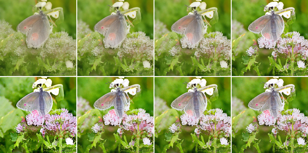
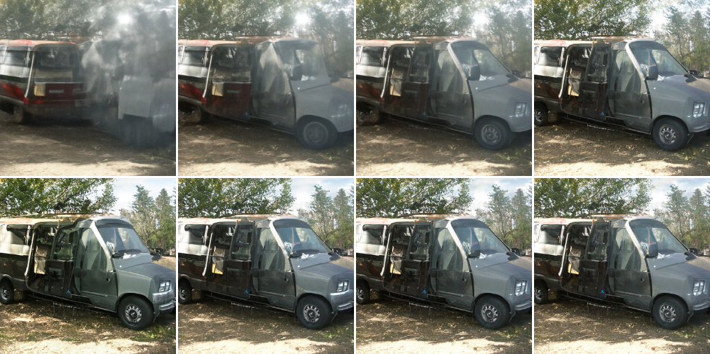
DPM-Solver can also be used for conditional sampling, with a simple modification. The conditional generation needs to sample from the conditional diffusion ODE [3, 4] which includes the conditional noise prediction model. We follow the classifier guidance method [4] to define the conditional noise prediction model as , where is a pre-trained classifier and is the classifier guidance scale (default is 1.0). Thus, we can use DPM-Solver to solve this diffusion ODE for fast conditional sampling, as shown in Fig. 1.
D.6 Numerical Stability
As we need to compute in the algorithm of DPM-Solver, we follow [10] to use expm1() instead of exp()-1 to improve numerical stability.
Appendix E Experiment Details
We test our method for sampling the most widely-used variance-preserving (VP) type DPMs [1, 2]. In this case, we have for all and . In spite of this, our method and theoretical results are general and independent of the choice of the noise schedule and .
For all experiments, we evaluate DPM-Solver on NVIDIA A40 GPUs. However, the computation resource can be other types of GPU, such as NVIDIA GeForce RTX 2080Ti, because we can tune the batch size for sampling.
E.1 Diffusion ODEs w.r.t.
Alternatively, the diffusion ODE can be reparameterized to the domain. In this section, we propose the formulation of diffusion ODEs w.r.t. for VP type, and other types can be similarly derived.
E.2 Code Implementation
We implement our code with both JAX (for continuous-time DPMs) and PyTorch (for discrete-time DPMs), and our code is released at https://github.com/LuChengTHU/dpm-solver.
E.3 Sample Quality Comparison with Continuous-Time Sampling Methods
| Sampling method NFE | 10 | 12 | 15 | 20 | 50 | 200 | 1000 | ||
|---|---|---|---|---|---|---|---|---|---|
| CIFAR-10 (continuous-time model (VP deep) [3], linear noise schedule) | |||||||||
| SDE | Euler (denoise) [3] | 304.73 | 278.87 | 248.13 | 193.94 | 66.32 | 12.27 | 2.44 | |
| 444.63 | 427.54 | 395.95 | 300.41 | 101.66 | 22.98 | 5.01 | |||
| Improved Euler [20] | 82.42(NFE=48), 2.73(NFE=151), 2.44(NFE=180) | ||||||||
| ODE | RK45 Solver [28, 3] | 19.55(NFE=26), 17.81(NFE=38), 3.55(NFE=62) | |||||||
| 51.66(NFE=26), 21.54(NFE=38), 12.72(NFE=50), 2.61(NFE=62) | |||||||||
| DPM-Solver (ours) | 4.70 | 3.75 | 3.24 | 3.99 | 3.84 (NFE = 42) | ||||
| 6.96 | 4.93 | 3.35 | 2.87 | 2.59 (NFE = 51) | |||||
Table 3 shows the detailed FID results, which is corresponding to Fig. 2(a). We use the official code and checkpoint in [3], the code license is Apache License 2.0. We use their released “checkpoint_8” of the “VP deep” type. We compare methods for and . We find that the sampling methods based on diffusion SDEs can achieve better sample quality with ; and that the sampling methods based on diffusion ODEs can achieve better sample quality with . For DPM-Solver, we find that DPM-Solver with less than 15 NFE can achieve better FID with than , while DPM-Solver with more than 15 NFE can achieve better FID with than .
For the diffusion SDEs with Euler discretization, we use the PC sampler in [3] with “euler_maruyama” predictor and no corrector, which uses uniform time steps between and . We add the “denoise” trick at the final step, which can greatly improve the FID score for .
For the diffusion SDEs with Improved Euler discretization [20], we follow the results in their original paper, which only includes the results with . The corresponding relative tolerance are , and , respectively.
For the diffusion ODEs with RK45 Solver, we use the code in [3], and tune the atol and rtol of the solver. For the NFE from small to large, we use the same atol = rtol = , , for the results of , and the same atol = rtol = , , , , for the results of , respectively.
E.4 Sample Quality Comparison with RK Methods
Table 1 shows the different performance of RK methods and DPM-Solver-2 and 3. We list the detailed settings in this section.
Assume we have an ODE with
Starting with at time , we use RK2 to approximate the solution at time in the following formulation (which is known as the explicit midpoint method):
And we use the following RK3 to approximate the solution at time (which is known as “Heun’s third-order method”), because it is very similar to our proposed DPM-Solver-3:
E.5 Sample Quality Comparison with Discrete-Time Sampling Methods
| Sampling method NFE | 10 | 12 | 15 | 20 | 50 | 200 | 1000 | |
| CIFAR-10 (discrete-time model [2], linear noise schedule) | ||||||||
| DDPM [2] | Discrete | 278.67 | 246.29 | 197.63 | 137.34 | 32.63 | 4.03 | 3.16 |
| Analytic-DDPM [21] | Discrete | 35.03 | 27.69 | 20.82 | 15.35 | 7.34 | 4.11 | 3.84 |
| Analytic-DDIM [21] | Discrete | 14.74 | 11.68 | 9.16 | 7.20 | 4.28 | 3.60 | 3.86 |
| †GGDM [18] | Discrete | 8.23 | 6.12 | 4.72 | ||||
| DDIM [19] | Discrete | 13.58 | 11.02 | 8.92 | 6.94 | 4.73 | 4.07 | 3.95 |
| DPM-Solver (Type-1 discrete) | 6.37 | 4.65 | 3.78 | 4.28 | 3.90 (NFE = 44) | |||
| 11.32 | 7.31 | 4.75 | 3.80 | 3.57 (NFE = 46) | ||||
| DPM-Solver (Type-2 discrete) | 6.42 | 4.86 | 4.39 | 5.52 | 5.22 (NFE = 42) | |||
| 10.16 | 6.26 | 4.17 | 3.72 | 3.48 (NFE = 44) | ||||
| CelebA 6464 (discrete-time model [19], linear noise schedule) | ||||||||
| DDPM [2] | Discrete | 310.22 | 277.16 | 207.97 | 120.44 | 29.25 | 3.90 | 3.50 |
| Analytic-DDPM [21] | Discrete | 28.99 | 25.27 | 21.80 | 18.14 | 11.23 | 6.51 | 5.21 |
| Analytic-DDIM [21] | Discrete | 15.62 | 13.90 | 12.29 | 10.45 | 6.13 | 3.46 | 3.13 |
| DDIM [19] | Discrete | 10.85 | 9.99 | 7.78 | 6.64 | 5.23 | 4.78 | 4.88 |
| DPM-Solver (Type-1 discrete) | 7.15 | 5.51 | 4.28 | 4.40 | 4.23 (NFE = 36) | |||
| 6.92 | 4.20 | 3.05 | 2.82 | 2.71 (NFE = 36) | ||||
| DPM-Solver (Type-2 discrete) | 7.33 | 6.23 | 5.85 | 6.87 | 6.68 (NFE = 36) | |||
| 5.83 | 3.71 | 3.11 | 3.13 | 3.10 (NFE = 36) | ||||
| ImageNet 6464 (discrete-time model [16], cosine noise schedule) | ||||||||
| DDPM [2] | Discrete | 305.43 | 287.66 | 256.69 | 209.73 | 83.86 | 28.39 | 17.58 |
| Analytic-DDPM [21] | Discrete | 60.65 | 53.66 | 45.98 | 37.67 | 22.45 | 17.16 | 16.14 |
| Analytic-DDIM [21] | Discrete | 70.62 | 54.88 | 41.56 | 30.88 | 19.23 | 17.49 | 17.57 |
| †GGDM [18] | Discrete | 37.32 | 24.69 | 20.69 | ||||
| DDIM [19] | Discrete | 67.07 | 52.69 | 40.49 | 30.67 | 20.10 | 17.84 | 17.73 |
| DPM-Solver (Type-1 discrete) | 24.44 | 20.03 | 19.31 | 18.59 | 17.50 (NFE = 48) | |||
| 27.74 | 23.66 | 20.09 | 19.06 | 17.56 (NFE = 51) | ||||
| DPM-Solver (Type-2 discrete) | 24.40 | 19.97 | 19.23 | 18.53 | 17.47 (NFE = 57) | |||
| 27.72 | 23.75 | 20.02 | 19.08 | 17.62 (NFE = 48) | ||||
| Sampling method NFE | 10 | 12 | 15 | 20 | 50 | 100 | 250 | |
|---|---|---|---|---|---|---|---|---|
| ImageNet 128128 (discrete-time model [4], linear noise schedule, classifier guidance scale: 1.25) | ||||||||
| DDPM [2] | Discrete | 199.56 | 172.09 | 146.42 | 119.13 | 49.38 | 23.27 | 2.97 |
| DDIM [19] | Discrete | 11.12 | 9.38 | 8.22 | 7.15 | 5.05 | 4.18 | 3.54 |
| DPM-Solver (Type-1 discrete) | 7.32 | 4.08 | 3.60 | 3.89 | 3.63 | 3.62 | 3.63 | |
| 13.91 | 5.84 | 4.00 | 3.52 | 3.13 | 3.10 | 3.09 | ||
| LSUN bedroom 256256 (discrete-time model [4], linear noise schedule) | ||||||||
| DDPM [2] | Discrete | 274.67 | 251.26 | 224.88 | 190.14 | 82.70 | 34.89 | †2.02 |
| DDIM [19] | Discrete | 10.05 | 7.51 | 5.90 | 4.98 | 2.92 | 2.30 | 2.02 |
| DPM-Solver (Type-1 discrete) | 6.10 | 4.29 | 3.30 | 3.09 | 2.53 | 2.46 | 2.46 | |
| 8.04 | 4.21 | 2.94 | 2.60 | 2.01 | 1.95 | 1.94 | ||
We compare DPM-Solver with other discrete-time sampling methods for DPMs, as shown in Table 4 and Table 5. We use the code in [19] for sampling with DDPM and DDIM, and the code license is MIT License. We use the code in [21] for sampling with Analytic-DDPM and Analytic-DDIM, whose license is unknown. We directly follow the best results in the original paper of GGDM [18].
For the CIFAR-10 experiments, we use the pretrained checkpoint by [2], which is also provided in the released code in [19]. We use quadratic time steps for DDPM and DDIM, which empirically has better FID performance than the uniform time steps [19]. We use the uniform time steps for Analytic-DDPM and Analytic-DDIM. For DPM-Solver, we use both Type-1 discrete and Type-2 discrete methods to convert the discrete-time model to the continuous-time model. We use the method in Appendix D.3 for NFE , and the adaptive step size solver in Appendix C for NFE . For all the experiments, we use DPM-Solver-12 with relative tolerance .
For the CelebA 64x64 experiments, we use the pretrained checkpoint by [19]. We use quadratic time steps for DDPM and DDIM, which empirically has better FID performance than the uniform time steps [19]. We use the uniform time steps for Analytic-DDPM and Analytic-DDIM. For DPM-Solver, we use both Type-1 discrete and Type-2 discrete methods to convert the discrete-time model to the continuous-time model. We use the method in Appendix D.3 for NFE , and the adaptive step size solver in Appendix C for NFE . For all the experiments, we use DPM-Solver-12 with relative tolerance . Note that our best FID results on CelebA 64x64 is even better than the 1000-step DDPM (and all the other methods).
For the ImageNet 64x64 experiments, we use the pretrained checkpoint by [16], and the code license is MIT License. We use the uniform time steps for DDPM and DDIM, following [19]. We use the uniform time steps for Analytic-DDPM and Analytic-DDIM. For DPM-Solver, we use both Type-1 discrete and Type-2 discrete methods to convert the discrete-time model to the continuous-time model. We use the method in Appendix D.3 for NFE , and the adaptive step size solver in Appendix C for NFE . For all the experiments, we use DPM-Solver-23 with relative tolerance . Note that the ImageNet dataset includes real human photos and it may have privacy issues, as discussed in [42].
For the ImageNet 128x128 experiments, we use classifier guidance for sampling with the pretrained checkpoints (for both the diffusion model and the classifier model) by [4], and the code license is MIT License. We use the uniform time steps for DDPM and DDIM, following [19]. For DPM-Solver, we only use Type-1 discrete method to convert the discrete-time model to the continuous-time model. We use the method in Appendix D.3 for NFE , and the adaptive step size solver DPM-Solver-12 with relative tolerance (detailed in Appendix C) for NFE . For all the experiments, we set the classifier guidance scale , which is the best setting for DDIM in [4] (we refer to their Table 14 for details).
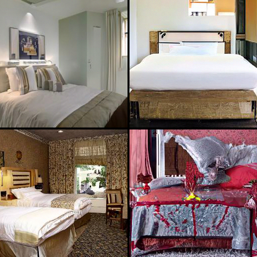
For the LSUN bedroom 256x256 experiments, we use the unconditional pretrained checkpoint by [4], and the code license is MIT License. We use the uniform time steps for DDPM and DDIM, following [19]. For DPM-Solver, we only use Type-1 discrete method to convert the discrete-time model to the continuous-time model. We use the method in Appendix D.3 for DPM-Solver.
E.6 Comparing Different Orders of DPM-Solver
We also compare the sample quality of the different orders of DPM-Solver, as shown in Table 6. We use DPM-Solver-1,2,3 with uniform time steps w.r.t. , and the fast version in Appendix D.3 for NFE less than 20, and we name it as DPM-Solver-fast. For the discrete-time models, we only compare the Type-2 discrete method, and the results of Type-1 are similar.
As the actual NFE of DPM-Solver-2 is and the actual NFE of DPM-Solver-3 is , which may be smaller than NFE, we use the notation † to note that the actual NFE is less than the given NFE. We find that for NFE less than 20, the proposed fast version (DPM-Solver-fast) is usually better than the single order method, and for larger NFE, DPM-Solver-3 is better than DPM-Solver-2, and DPM-Solver-2 is better than DPM-Solver-1, which matches our proposed convergence rate analysis.
| Sampling method NFE | 10 | 12 | 15 | 20 | 50 | 200 | 1000 | |
|---|---|---|---|---|---|---|---|---|
| CIFAR-10 (VP deep continuous-time model [3]) | ||||||||
| DPM-Solver-1 | 11.83 | 9.69 | 7.78 | 6.17 | 4.28 | 3.85 | 3.83 | |
| DPM-Solver-2 | 5.94 | 4.88 | †4.30 | 3.94 | 3.78 | 3.74 | 3.74 | |
| DPM-Solver-3 | †18.37 | 5.53 | 4.08 | †4.04 | †3.81 | †3.78 | †3.78 | |
| DPM-Solver-fast | 4.70 | 3.75 | 3.24 | 3.99 | ||||
| DPM-Solver-1 | 11.29 | 9.07 | 7.15 | 5.50 | 3.32 | 2.72 | 2.64 | |
| DPM-Solver-2 | 7.30 | 5.28 | †4.23 | 3.26 | 2.69 | 2.60 | 2.59 | |
| DPM-Solver-3 | †54.56 | 6.03 | 3.55 | †2.90 | †2.65 | †2.62 | †2.62 | |
| DPM-Solver-fast | 6.96 | 4.93 | 3.35 | 2.87 | ||||
| CIFAR-10 (DDPM discrete-time model [2]), DPM-Solver with Type-2 discrete | ||||||||
| DPM-Solver-1 | 16.69 | 13.63 | 11.08 | 8.90 | 6.24 | 5.44 | 5.29 | |
| DPM-Solver-2 | 7.90 | 6.15 | †5.53 | 5.24 | 5.23 | 5.25 | 5.25 | |
| DPM-Solver-3 | †24.37 | 8.20 | 5.73 | †5.43 | †5.29 | †5.25 | †5.25 | |
| DPM-Solver-fast | 6.42 | 4.86 | 4.39 | 5.52 | ||||
| DPM-Solver-1 | 13.61 | 10.98 | 8.71 | 6.79 | 4.36 | 3.63 | 3.49 | |
| DPM-Solver-2 | 11.80 | 6.31 | †5.23 | 3.95 | 3.50 | 3.46 | 3.46 | |
| DPM-Solver-3 | †67.02 | 9.45 | 5.21 | †3.81 | †3.49 | †3.45 | †3.45 | |
| DPM-Solver-fast | 10.16 | 6.26 | 4.17 | 3.72 | ||||
| CelebA 6464 (discrete-time model [19], linear noise schedule), DPM-Solver with Type-2 discrete | ||||||||
| DPM-Solver-1 | 18.66 | 16.30 | 13.92 | 11.84 | 8.85 | 7.24 | 6.93 | |
| DPM-Solver-2 | 5.89 | 5.83 | †6.08 | 6.38 | 6.78 | 6.84 | 6.85 | |
| DPM-Solver-3 | †11.45 | 5.46 | 6.18 | †6.51 | †6.87 | †6.84 | †6.85 | |
| DPM-Solver-fast | 7.33 | 6.23 | 5.85 | 6.87 | ||||
| DPM-Solver-1 | 13.24 | 11.13 | 9.08 | 7.24 | 4.50 | 3.48 | 3.25 | |
| DPM-Solver-2 | 4.28 | 3.40 | †3.30 | 3.17 | 3.19 | 3.20 | 3.20 | |
| DPM-Solver-3 | †49.48 | 3.84 | 3.09 | †3.15 | †3.20 | †3.20 | †3.20 | |
| DPM-Solver-fast | 5.83 | 3.71 | 3.11 | 3.13 | ||||
| ImageNet 6464 (discrete-time model [16], cosine noise schedule), DPM-Solver with Type-2 discrete | ||||||||
| DPM-Solver-1 | 32.84 | 28.54 | 24.79 | 21.71 | 18.30 | 17.45 | 17.18 | |
| DPM-Solver-2 | 29.20 | 24.97 | †22.26 | 19.94 | 17.79 | 17.29 | 17.27 | |
| DPM-Solver-3 | †57.48 | 24.62 | 19.76 | †18.95 | †17.52 | 17.26 | 17.27 | |
| DPM-Solver-fast | 24.40 | 19.97 | 19.23 | 18.53 | ||||
| DPM-Solver-1 | 32.31 | 28.44 | 25.15 | 22.38 | 19.14 | 17.95 | 17.44 | |
| DPM-Solver-2 | 33.16 | 27.28 | †24.26 | 20.58 | 18.04 | 17.46 | 17.41 | |
| DPM-Solver-3 | †162.27 | 27.28 | 22.38 | †19.39 | †17.71 | †17.43 | †17.41 | |
| DPM-Solver-fast | 27.72 | 23.75 | 20.02 | 19.08 | ||||
E.7 Runtime Comparison between DPM-Solver and DDIM
Theoretically, for the same NFE, the runtime of DPM-Solver and DDIM are almost the same (linear to NFE) because the main computation costs are the serial evaluations of the large neural network and the other coefficients are analytically computed with ignorable costs.
Table 7 shows the runtime of DPM-Solver and DDIM on a single NVIDIA A40, varying different datasets and NFE. We use torch.cuda.Event and torch.cuda.synchronize for accurately computing the runtime. We use the discrete-time pretrained diffusion models for each dataset. We evaluate the runtime for 8 batches and computes the mean and std of the runtime. We use 64 batch size for LSUN bedroom 256x256 due to the GPU memory limitation, and 128 batch size for other datasets.
For DDIM, we use the official implementation222https://github.com/ermongroup/ddim. We find that our implementation of DPM-Solver reduces some repetitive computation of the coefficients, so under the same NFE, DPM-Solver is slightly faster than DDIM of their implementation. Nevertheless, the runtime evaluation results show that the runtime of DPM-Solver and DDIM are almost the same for the same NFE, and the runtime is approximately linear to the NFE. Therefore, the speedup for the NFE is almost the actual speedup of the runtime, so the proposed DPM-Solver can greatly speedup the sampling of DPMs.
| Sampling method NFE | 10 | 20 | 50 | 100 |
|---|---|---|---|---|
| CIFAR-10 3232 (batch size = 128) | ||||
| DDIM | 0.956(0.011) | 1.924(0.016) | 4.838(0.024) | 9.668(0.013) |
| DPM-Solver | 0.923(0.006) | 1.833(0.004) | 4.580(0.005) | 9.204(0.011) |
| CelebA 6464 (batch size = 128) | ||||
| DDIM | 3.253(0.015) | 6.438(0.029) | 16.132(0.050) | 32.255(0.044) |
| DPM-Solver | 3.126(0.003) | 6.272(0.006) | 15.676(0.008) | 31.269(0.012) |
| ImageNet 6464 (batch size = 128) | ||||
| DDIM | 5.084(0.018) | 10.194(0.022) | 25.440(0.044) | 50.926(0.042) |
| DPM-Solver | 4.992(0.004) | 9.991(0.003) | 24.948(0.007) | 49.835(0.028) |
| ImageNet 128128 (batch size = 128, with classifier guidance) | ||||
| DDIM | 29.082(0.015) | 58.159(0.012) | 145.427(0.011) | 290.874(0.134) |
| DPM-Solver | 28.865(0.011) | 57.645(0.008) | 144.124(0.035) | 288.157(0.022) |
| LSUN bedroom 256256 (batch size = 64) | ||||
| DDIM | 37.700(0.005) | 75.316(0.013) | 188.275(0.172) | 378.790(0.105) |
| DPM-Solver | 36.996(0.039) | 73.873(0.023) | 184.590(0.010) | 369.090(0.076) |
E.8 Conditional Sampling on ImageNet 256x256
For the conditional sampling in Fig. 1, we use the pretrained checkpoint in [4] with classifier guidance (ADM-G), and the classifier scale is . The code license is MIT License. We use uniform time step for DDIM, and the fast version for DPM-Solver in Appendix D.3 (DPM-Solver-fast) with 10, 15, 20 and 100 steps.
Fig. 3 shows the conditional sample results by DDIM and DPM-Solver. We find that DPM-Solver with 15 NFE can generate comparable samples with DDIM with 100 NFE.
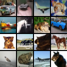
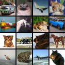
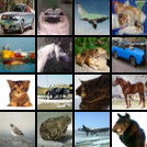
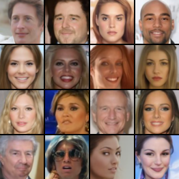
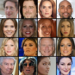
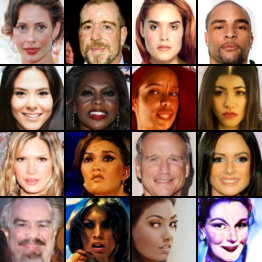
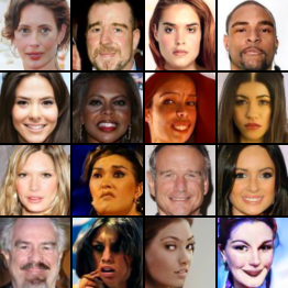
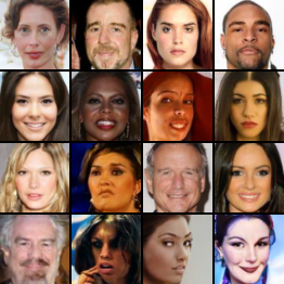
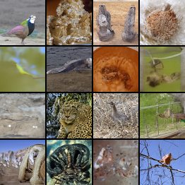
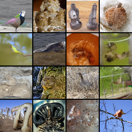
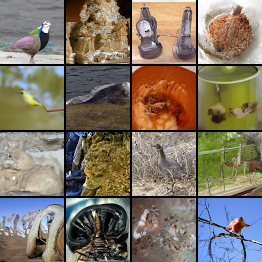
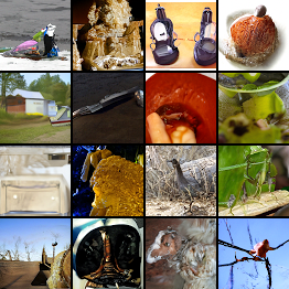
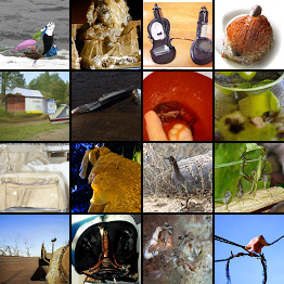
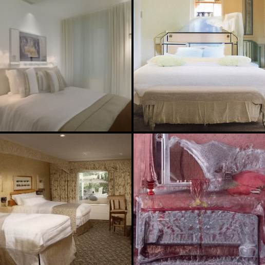
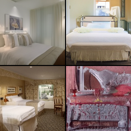
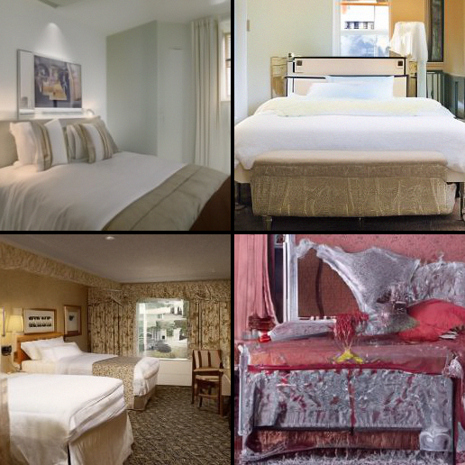
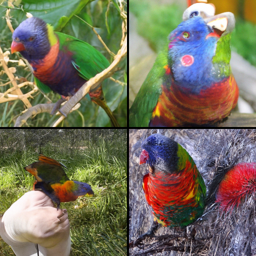
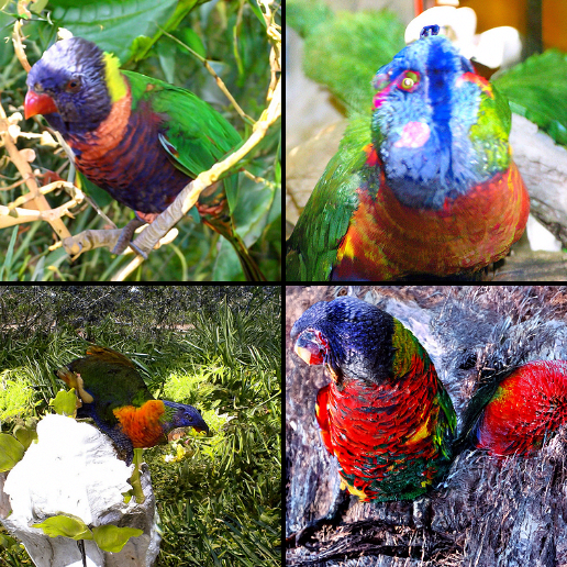
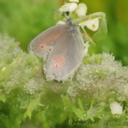
E.9 Additional Samples
Additional sampling results on CIFAR-10, CelebA 64x64, ImageNet 64x64, LSUN bedroom 256x256 [40], ImageNet 256x256 are reported in Figs. 4-8.