Mean Escape Time of Switched Riccati Differential Equations

Abstract

Riccati differential equations is the class of first-order and quadratic ordinary differential equations and has various applications in the systems and control theory. In this paper, we analyze a switched Riccati differential equation that is driven by a Poisson-like stochastic signal. We specifically focus on the computation of the mean escape time of the switched Riccati differential equation. The contribution of this paper is twofold. We first show that, under the assumption that the subsystems described as a deterministic Riccati differential equation escape in finite time regardless of its initial state, the mean escape time of the switched Riccati differential equation admits a power series expression. In order to further expand the applicability of this result, we then present an approximative formula for computing the escape time of deterministic Riccati differential equations. We present numerical simulations to illustrate the obtained results.

[OU]organization=Graduate School of Information Science and Technology, Osaka University,addressline=Yamadaoka 1-5, city=Suita, postcode=565-0871, state=Osaka, country=Japan

[TTU]organization=Department of Mathematics and Statistics, Texas Tech University,addressline=1108 Memorial Circle, city=Lubbock, postcode=79409, state=TX, country=USA

1 Introduction

Riccati differential equations (RDEs) [1] is the class of first-order and quadratic ordinary differential equations and has various applications in dynamic games [2], $H^{\infty}$ optimal control problems [3], and singular perturbation of boundary value problems [4]. For a recent survey of RDEs, see [5] and the references therein. For the specific case of scalar RDEs, we refer the readers to the classic work by Watson [6]. Although it is well-known that a Riccati differential equation is locally equivalent to a linear ordinary differential equation by a change of basis [1], the non-linearlity of a RDE allows its solution to diverge in a finite time, which is called the finite-time escape phenomena. Various characterizations and conditions for the finite-time escape phenomena can be found in the literature (see, e.g., [7, 8, 9]). Among the various results, the most fundamental fact is that the finite-time escape can be characterized by the leave of the induced flow on a manifold called the Grassmannian [1, 10] from its canonical chart. As for the qualitative analysis of the finite-time escape phenomena, Getz and Jacobson [11] derive a sufficient condition for the solution to escape in a finite time, and also give an upper bound of the escape time. On the other hand, Freiling et al. [12] give a condition under which a finite-time escape phenomena does not occur.

The primary objective of this paper is investigating the escape time of switched RDEs, in which its subsystems are described by RDEs, and its switching dynamics is driven by a Poisson-like stochastic signal. It can be easily confirmed that a switched linear system with Poisson jumps is a Markov jump linear system, which is widely studied in the literature (see, e.g., [13, 14, 15, 16]). Although we can find extensive amount of works for studying the Markov jump nonlinear systems [17, 18, 19, 20], most of them implicitly assume the non-existence of the finite-time escape in each of the subsystems. Therefore, these results available in the literature for Markov jump nonlinear systems are not directly applicable to switched RDEs studied in this paper.

To fill in the aforementioned gap, in this paper, we first study the computation of the mean escape time of a switched RDE subject to Poisson switching. Specifically, under the assumption that its subsystems described by deterministic RDEs escape in finite time regardless of their initial states, we show that the mean escape time of the switched RDE admits a power series expression. In order to further expand the applicability of this result, we then present an approximative formula for the computation of the escape time of deterministic RDEs.

This paper is organized as follows. After preparing necessary mathematical notation and conventions, in Section 2 we briefly review the RDEs and Grassmannians and, then, introduce the switched RDEs subject to Poisson switching. Then, in Section 3, we study the expected value of the escape time of switched RDEs. We then study the approximate computation of the escape time of both deterministic and switched RDEs in Section 4. We finally conclude the paper in Section 5.

1.1 Notation

We let the field of real numbers be denoted by $\mathbb{R}$. For a positive number $x$, we define $\log^{+}(x)=\max(\log x,0)$. For a subset $S$ on $\mathbb{R}$, we let $\chi_{S}$ denote the characteristic function of $S$. product in $\mathbb{R}^{d}$, which yields The Euclidean norm of a real vector $v$ is denoted by $\lVert v\rVert$. We also define the norm $\lVert v\rVert_{\infty}=\max_{i=1}^{d}\lvert v_{i}\rvert$. We denote by $I_{n}$ the identity matrix of the dimension $n$. The subscript $n$ will be omitted when it is clear from the context. The maximum singular value of a matrix $M\in\mathbb{R}^{m\times d}$ is denoted by $\lVert M\rVert$. We let $\operatorname{Sp}M$ denote the column space of $M$. When $M$ is square, we let $\operatorname{tr}M$ denote the trace of $M$. For a subspace $V$ in $\mathbb{R}^{d}$, we define the subspace $M(V)$ of $\mathbb{R}^{m}$ by $M(V)=\{Mv:v\in V\}$. Let $\operatorname{Gl}(d,\mathbb{R})$ denote the multiplicative group of invertible $d\times d$ real matrices. The subgroup of $\operatorname{Gl}(d,\mathbb{R})$ consisting of the matrices having determinant $1$ is denoted by $\operatorname{Sl}(d,\mathbb{R})$.

For a measure space $X$, we let $L^{\infty}(X)^{n}$ denote the set of $\mathbb{R}^{n}$-valued Lebesgue measurable functions $f$ on $X$ satisfying $\sup_{x\in X}\lVert f(x)\rVert_{\infty}<\infty$. The set $L^{\infty}(X)^{n}$ becomes a Banach space when equipped with the norm $\lVert f\rVert=\sup_{x\in X}\lVert f(x)\rVert_{\infty}$.

Let $X$ be metric space with a distance $\rho$. A subset $N\subset X$ is called an $\epsilon$-net of $X$ if for every $x\in X$ there exists $y\in N$ such that $\rho(x,y)<\epsilon$. $X$ is called totally bounded if $X$ admits a finite $\epsilon$-net for every $\epsilon>0$.

For a Banach space $X$, let $\mathcal{L}(X)$ denote the space of continuous linear operators on $X$. The identity operator in $\mathcal{L}(X)$ is denoted by $I$. The set $\mathcal{L}(X)$ becomes a Banach space when equipped with the norm $\lVert A\rVert=\sup_{x\neq 0}{\lVert Ax\rVert}/{\lVert x\rVert}$. The next lemma about the invertibility of the operators in $\mathcal{L}(X)$ is well known.

Lemma 1.1

Let $X$ be a Banach space. Take an arbitrary $A\in\mathcal{L}(X)$. Assume $\lVert A\rVert<1$. Then, the operator $I-A$ is invertible in $\mathcal{L}(X)$ and, furthermore, the inverse equals $\sum_{k=0}^{\infty}A^{k}$.

Let us also state a matrix version of Lemma 1.1.

Lemma 1.2

Let $M$ be a square matrix.

1. If $\lVert M-I\rVert<1$, then $M$ is invertible.

2. If $\lVert M\rVert<1$, then the matrix $I-M$ is invertible and, moreover, $\lVert(I-M)^{-1}\rVert\leq 1/(1-\lVert M\rVert)$.

2 Switched Riccati Differential Equations

In this section, we introduce the RDE with Poisson jumps. In Subsection 2.1, we briefly review RDEs with an emphasis on their relationship to Grassmannian manifolds. Then, in Subsection 2.2, we formulate RDEs with Poisson jumps, which is the main subject of this paper.

2.1 RDEs and Grassmannians

Let us give a brief review on RDEs and their relationship to Grassmannians [1]. Take an arbitrary matrix $A\in\mathbb{R}^{d\times d}$. Let $k<d$ be a positive integer. Partition the matrix $A$ as

$$A=\begin{bmatrix}A_{11}&A_{12}\\ A_{21}&A_{22}\end{bmatrix},$$

for $A_{11}\in\mathbb{R}^{k\times k}$, $A_{12}\in\mathbb{R}^{k\times(d-k)}$, $A_{21}\in\mathbb{R}^{(d-k)\times k}$, and $A_{22}\in\mathbb{R}^{(d-k)\times(d-k)}$. Then, we can define the Riccati differential equation (RDE) associated with the matrix $A$ by

$$\frac{dY}{dt}=A_{21}+A_{22}Y-YA_{11}-YA_{12}Y.$$ (1)

We remark that this RDE is not necessarily symmetric because the matrix $A$ is taken arbitrarily. Now, we let the solution of this RDE with the initial condition $Y(0)=Y_{0}$ by $Y(\cdot;Y_{0})$. Then, the first time $t>0$ at which the solution $Y(t;Y_{0})$ does not exist is defined as the escape time [7] of the RDE (1). When such $t$ does not exist, i.e., if the solution of the RDE (1) exists for all $t\geq 0$, then we regard the escape time of the RDE as $+\infty$.

RDEs are closely related to manifolds called Grassmannians [1, 7]. Specifically, the Grassmannian $G^{k}(\mathbb{R}^{d})$ consists of the set of all the $k$-dimensional subspaces in $\mathbb{R}^{d}$. In the special case of $k=1$, the Grassmannian reduces to the real projective space and is denoted by $P(\mathbb{R}^{d})$. Notice that the group $\operatorname{Gl}(\mathbb{R}^{d})$ acts on the manifold $G^{k}(\mathbb{R}^{d})$ because an invertible matrix always maps a $k$-dimensional subspace to another $k$-dimensional subspace.

There exists a fundamental connection between the RDEs and the Grassmannians. Let us define $\psi\colon\mathbb{R}^{(d-k)\times k}\to G^{k}(\mathbb{R}^{d})$ by the equation

$$\psi(K)=\operatorname{Sp}\begin{bmatrix}I_{k}\\ K\end{bmatrix}.$$

We also define $G_{0}^{k}(\mathbb{R}^{d})\subset G^{k}(\mathbb{R}^{d})$ as the set of all the $k$-dimensional subspaces in $\mathbb{R}^{d}$ complementary to the subspace $\operatorname{Sp}\begin{bmatrix}0\\ I_{d-k}\end{bmatrix}$. Then, one can see that the mapping $\psi$ embeds the set $\mathbb{R}^{(d-k)\times k}$ into the Grassmannian $G^{k}(\mathbb{R}^{d})$ as the open and dense subset $G_{0}^{k}(\mathbb{R}^{d})$. Furthermore, one can show that the equation

$$\psi(Y(t;Y_{0}))=e^{At}(\psi(Y_{0}))$$ (2)

holds true whenever the solution $Y(t;Y_{0})$ of the RDE (1) exists. This equation implies that RDE (1) can be regarded as the local expression of the differential equation on $G^{k}(\mathbb{R}^{d})$ corresponding to the flow

$$F(t;F_{0})=e^{At}(F_{0})$$ (3)

with respect to the chart $(G_{0}^{k}(\mathbb{R}^{d}),\psi^{-1})$. Therefore, by the extended RDE (ERDE), we mean the differential equation on $G^{k}(\mathbb{R}^{d})$ having the flow (3). For this reason, with the abuse of notation, we write the solution of RDE (1) as

$$e^{At}.Y_{0}=Y(t;Y_{0}).$$ (4)

It should be noticed that, by the relationship (2), we can see that RDE (1) escapes exactly when the flow $e^{At}(\psi(Y_{0}))$ leaves the subset $G_{0}^{k}(\mathbb{R}^{d})$.

As for the escape time of the RDE (1), we can specifically see that the solution of (1) is given by $Y(t;Y_{0})=V(t)U(t)^{-1}$ where $U(t)\in\mathbb{R}^{k\times k}$ and $V(t)\in\mathbb{R}^{(d-k)\times k}$ are given by the partition

$$\begin{bmatrix}U(t)\\ V(t)\end{bmatrix}=e^{At}\begin{bmatrix}I_{n}\\ Y_{0}\end{bmatrix}$$ (5)

provided that $U(t)^{-1}$ exists. Hence, the equation (1) escapes precisely at the minimum $t\geq 0$ at which the matrix $U(t)$ becomes singular.

Let us see an example to fix ideas.

Example 2.1

Let $\omega$ be a positive number. Let us consider the RDE

$$\frac{dy}{dt}=\omega(1+y^{2}).$$ (6)

We set the initial condition of this RDE as $y(0)=0$. It is trivial to see that the solution of this RDE is given by $y(t)=\tan(\omega t)$. This implies that the RDE (6) escapes at the time $t=\pi/(2\omega)$. On the other hand, the ERDE induced by the RDE (6) can be derived as follows. First, to the domain $\mathbb{R}$ of the RDE (6), we can correspond the Grassmannian $G^{1}(\mathbb{R}^{2})$ (i.e., the projective space $P(\mathbb{R}^{2})$). Hence, the canonical chart $\psi$ maps a real number $t$ to the straight line having the slope $t$ and passing through the origin. This particularly implies that the initial state $y(0)=0$ of the RDE is mapped to the $x$-axis. Furthermore, with this canonical chart, a flow on $P(\mathbb{R}^{2})$ escapes exactly when it coincides with the $y$-axis. Now, because the RDE (6) is induced by the matrix

$$A=\begin{bmatrix}0&-\omega\\ \omega&0\end{bmatrix},$$

the ERDE is nothing but the flow described by

$$e^{At}.(\psi(0))=\left\{r\begin{bmatrix}\cos(\omega t)\\ \sin(\omega t)\end{bmatrix}:r\in\mathbb{R}\right\},$$

representing a straight line rotating with the angular speed $\omega$ counterclockwise. Therefore, starting initially from the $x$-axis, the flow escapes at time $\pi/(2\omega)$, which coincides with our finding above.

2.2 RDEs subject to Poisson switching

The objective of this paper is to study the escape time of switched RDEs subject to Poisson jumps, which we describe below. Let $A,B\in\mathbb{R}^{d\times d}$ and consider the RDE (1) and another RDE

$$\frac{dY}{dt}=B_{21}+B_{22}Y-YB_{11}-YB_{12}Y.$$ (7)

Although we focus on the case of two subsystems, most of the results presented in this paper can be extended to the case of more than two subsystems.

We define a $\{0,1\}$-valued random variable $z$ by the stochastic differential equation [21]

$$dz=(1-2z)dN,\quad z(0)\in\{0,1\}$$ (8)

where $N$ is the Poisson process of rate $\lambda>0$. The stochastic process $z$ is a continuous-time Markov process with switching rate $\lambda$.

Now, we consider the following RDE with Poisson jump:

$$\begin{multlined}dY=\left[z(A_{21}+A_{22}Y-YA_{11}-YA_{12}Y)+(1-z)(B_{21}+B_{22}Y-YB_{11}-YB_{12}Y)\right]dt.\end{multlined}dY=\left[z(A_{21}+A_{22}Y-YA_{11}-YA_{12}Y)+(1-z)(B_{21}+B_{22}Y-YB_{11}-YB_{12}Y)\right]dt.$$ (9)

Our major objective in this paper is in the numerical calculation and the theoretical characterization of the average escape time of the switched RDE (9). Specifically, let $Y_{0}\in\mathbb{R}^{(d-k)\times k}$ be arbitrary, and let $T_{A}(Y_{0})$ ($T_{B}(Y_{0})$) denote the mean escape time of the switched RDE (9) when $Y(0)=Y_{0}$ and $z(0)=1$ ($z(0)=0$, respectively). In Section 3, we show that the mean escape times admit a representation as a power series, under the assumption that the escape time of the deterministic RDEs (1) and (7) are analytically available. Then, in Section 4, we show that, even when the escape time of the deterministic RDEs are not available, we can still approximately compute the mean escape times.

3 Analytical Charecterization of Mean Escape Time

Let $t_{A}(Y_{0})$ and $t_{B}(Y_{0})$ denote the escape time of the deterministic RDEs (1) and (7). Throughout this section, we place the following assumption.

Assumption 3.1

Assume that there exists a constant $t_{0}>0$ such that

$$t_{i}(Y_{0})\leq t_{0}$$ (10)

for all $Y_{0}\in\mathbb{R}^{(d-k)\times k}$ and $i\in\{A,B\}$.

The main objective of this section is to prove the following theorem characterizing the mean escape time of the switched RDE (9).

Theorem 3.2

Define the probability distribution function $F(t)=\int_{0}^{t}f(\tau)\,d\tau$ ($t\geq 0$) associated with the probability density function $f(t)=\lambda e^{-\lambda t}$ ($t\geq 0$). Define the real valued functions $g_{1}$ and $g_{2}$ defined on $\mathbb{R}^{(d-k)\times k}$ by

$$g_{1}(Y) =\int_{0}^{t_{A}(Y)}\tau f(\tau)\,d\tau+t_{A}(Y)\left(1-F(t_{A}(Y))\right),$$

$$g_{2}(Y) =\int_{0}^{t_{B}(Y)}\tau f(\tau)\,d\tau+t_{B}(Y)\left(1-F(t_{B}(Y))\right).$$

Also, define the operators $M_{1}$ and $M_{2}$ acting on $L^{\infty}(\mathbb{R}^{(d-k)\times k})$ by

$$(M_{1}T)(Y) =\int_{0}^{t_{A}(Y)}f(\tau)T(e^{A\tau}.Y)\,d\tau,$$

$$(M_{2}T)(Y) =\int_{0}^{t_{B}(Y)}f(\tau)T(e^{B\tau}.Y)\,d\tau$$

for all $Y\in\mathbb{R}^{(d-k)\times k}$. Then, we have

$$\begin{bmatrix}T_{A}\\ T_{B}\end{bmatrix}=\sum^{\infty}_{k=0}M^{k}\begin{bmatrix}g_{1}\\ g_{2}\end{bmatrix},$$ (11)

where the operator $M$ is given by

$$M=\begin{bmatrix}0&M_{1}\\ M_{2}&0\end{bmatrix}.$$

Proof 1

Let us temporarily assume $z(0)=1$, i.e., let us suppose that the switched RDE (9) initially starts from the first subsystem given in (1). If no switch occurs after the initial time $t=0$, then the solution of the RDE would escape at $t=t_{A}(Y_{0})$ by the definition of the mapping $t_{A}$. On the other hand, suppose that the first switching occurs at a time $t=\tau$. This $\tau$ must satisfy $\tau<t_{A}(Y_{0})$. At this time instant, the solution of the switched RDE is equal to $e^{A\tau}.Y_{0}$ under the notation (4). Hence, by definition, the switched RDE will escape after $T_{B}(e^{A\tau}.Y_{0})$ time units in average. Summarizing this argument, we obtain the following integral equation:

$$\begin{multlined}T_{A}(Y_{0})=\int^{t_{A}(Y_{0})}_{0}f(\tau)[\tau+T_{B}(e^{A\tau}.Y_{0})]\,d\tau+\left(1-F(t_{A}(Y_{0}))\right)t_{A}(Y_{0}),\end{multlined}T_{A}(Y_{0})=\int^{t_{A}(Y_{0})}_{0}f(\tau)[\tau+T_{B}(e^{A\tau}.Y_{0})]\,d\tau+\left(1-F(t_{A}(Y_{0}))\right)t_{A}(Y_{0}),$$

which leads us to the functional equation $T_{A}=g_{1}+M_{1}T_{B}$. In the same way, we can derive the functional equation $T_{B}=g_{2}+M_{2}T_{A}$. Therefore, the mean escape times $T_{A}$ and $T_{B}$ satisfy

$$(I-M)\begin{bmatrix}T_{A}\\ T_{B}\end{bmatrix}=\begin{bmatrix}g_{1}\\ g_{2}\end{bmatrix}.$$

Hence, by Lemma 1.1, to complete the proof of the theorem, it is enough to show that the following claims hold true:

1. $M$ is a continuous linear operator on the space $L^{\infty}(\mathbb{R}^{(d-k)\times k})^{2}$;

2. There holds that $\lVert M\rVert<1$.

First, we can trivially confirm that $M$ is linear. To show its continuity, let us take arbitrary $T,T^{\prime}\in L^{\infty}(\mathbb{R}^{(d-k)\times k})$. Then, we can show

$$\left\lVert M\begin{bmatrix}T\\ T^{\prime}\end{bmatrix}\right\rVert =\sup_{W\in\mathbb{R}^{(d-k)\times k}}\left\lVert M\begin{bmatrix}T\\ T^{\prime}\end{bmatrix}(Y)\right\rVert_{\infty}$$

$$=\sup_{W\in\mathbb{R}^{(d-k)\times k}}\left\lVert\begin{bmatrix}(M_{1}T^{\prime})(Y)\\ (M_{2}T)(Y)\end{bmatrix}\right\rVert_{\infty}.$$ (12)

Hence, for every $Y\in\mathbb{R}^{(d-k)\times k}$, we can show

$$\left|(M_{1}T^{\prime})(Y)\right| =\left|\int_{0}^{t_{A}(Y)}f(\tau)T^{\prime}(e^{A\tau}.Y)\,d\tau\right|$$

$$\leq\int_{0}^{t_{A}(Y)}f(\tau)\lvert T^{\prime}(e^{A\tau}.Y)\rvert\,d\tau$$

$$\leq\sup_{W\in\mathbb{R}^{(d-k)\times k}}{\lvert T^{\prime}(Y)\rvert}\int_{0}^{t_{0}}f(\tau)\,d\tau$$

$$=\lVert T^{\prime}\rVert F(t_{0}).$$ (13)

In the same way we can show

$$\left|(M_{2}T)(Y)\right|\leq\lVert T\rVert F(t_{0}).$$ (14)

The equation (12) together with (13) and (14) yield

$$\left\lVert M\begin{bmatrix}T\\ T^{\prime}\end{bmatrix}\right\rVert \leq F(t_{0})\left\lVert\begin{bmatrix}\lVert T^{\prime}\rVert\\ \lVert T\rVert\end{bmatrix}\right\rVert_{\infty}$$

$$=F(t_{0})\left\lVert\begin{bmatrix}T\\ T^{\prime}\end{bmatrix}\right\rVert.$$ (15)

Therefore, we conclude that $M$ is a continuous linear operator. Furthermore, the second claim b) follows immediately from inequality (15) because we know $F(t_{0})<1$. This completes the proof.

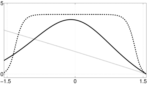
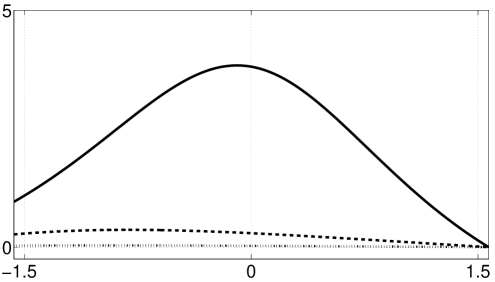
Figure 1: Expected value $T_{A}$ of the escape time when $\gamma=\lambda=1$. Solid: $\omega=1$, Dashed: $\omega=10$, Dotted: $\omega=100$.

Figure 2: Expected value $T_{A}$ of the escape time when $\omega=\gamma=1$. Solid: $\lambda=1$, Dashed: $\lambda=10$, Dotted: $\lambda=0.01$.

Let us see an example.

Example 3.3

Let $\omega$ and $\gamma$ be positive numbers. In this example, we consider the following switched RDE

$$dy=\left[z\left(\omega(1+y^{2})\right)+(1-z)\left(-\gamma(1+y^{2})\right)\right]dt,$$ (16)

where $z$ is the stochastic process defined by the stochastic differential equation (8). This switched RDE consists of the RDE (6) and the following RDE:

$$\frac{dy}{dt}=-\gamma(1+y^{2}).$$ (17)

By regarding the RDEs as the local expressions of the rotations in $G^{1}(\mathbb{R}^{2})$ with the angular speeds $\omega$ and $-\gamma$, we can find

$$t_{A}(\theta)=\frac{(\pi/2)-\theta}{\omega},\quad t_{B}(\theta)=\frac{\theta+(\pi/2)}{\gamma}$$

where an element in $G^{1}(\mathbb{R}^{2})$ is identified with its angle $\theta$ measured from the positive $x$-axis. This implies that the assumption (10) is satisfied with the constant $t_{0}=\max\{\pi/\omega,\pi/\gamma\}$.

We now use Theorem 3.2 to find the mean escape time of the switched RDE (16). First, we fix $\gamma=\lambda=1$ and change $\omega$ as $\omega=1$, $10$, and $100$. In Fig. 2, we show the mean escape time $T_{A}$ as a function of the initial angle $\theta_{0}\in[-\pi/2,\pi/2]$. The mean escape time in the figure is obtained by terminating the power series (11) at its 21st term. It can be observed that the mean escape time decreases in $\omega$. This is because, the larger $\omega$, the earlier the rotation of the line to pass the critical line of $y$-axis, at which an escape occurs. We then fix $\omega=\gamma=1$ and observe how the mean escape time depends on the switching rate $\lambda$. In fig. 2, we show the mean escape time $T_{A}$ for $\lambda=0.01$, $1$, and $10$. When $\lambda=0.01$, the mean escape time is close to the escape time of the deterministic RDE (6). This is because, when the rate $\lambda$ is small, a switching from the first RDE (6) to the second RDE (17) rarely occurs and, hence, the presence of switching is negligible.

4 Approximate Computation of Mean Escape Time

One of the potential difficulties in using the analytic formula in Theorem 3.2 to compute the mean escape time of switched RDE (9) is in computing the escape time of deterministic RDEs (1) and (7). For example, consider the RDE (1) on $\mathbb{R}^{1\times 2}$ determined by the matrix

$$A=T^{-1}\begin{bmatrix}0&1&0\\ -1&0&0\\ 0&0&1\end{bmatrix}T,\quad T=\begin{bmatrix}1&0&1\\ 0&1&0\\ 0&0&1\end{bmatrix}$$

with the initial state

$$Y_{0}=\begin{bmatrix}1\\ 1\end{bmatrix}.$$

We can show that the corresponding ERDE is the flow

$$e^{At}\left(\psi(Y_{0})\right)=\left\{r\begin{bmatrix}2\cos t+\sin t-e^{t}\\ \cos t-2\sin t\\ e^{t}\end{bmatrix}:r\in\mathbb{R}\right\}$$

in $P(\mathbb{R}^{3})$. Therefore, under the canonical chart $\psi$, this RDE escapes when $2\cos t+\sin t-e^{t}=0$. However it is not easy to calculate the zeros of this type of transcendental equation effectively.

The objective of this section is to provide an approximative method to compute the mean escape time of the switched RDE (9). In Subsection 4.1, we propose a method to approximately compute the escape time of the deterministic RDEs. Although this method allows us to use Theorem 3.2 to approximately compute the mean escape time of the switched RDE (9), it is not clear if the computation is robust with respect to the computational error of the escape time of the deterministic RDEs. Therefore, in Subsection 4.2, we present a theorem confirming the computational robustness.

4.1 Sequence converging to escape time

In this section, we give a procedure for approximately computing the escape time of deterministic RDEs. We remark that, although there are many results concerning the occurrence of finite-time escape phenomenon, the computation of escape time has not attracted much attention. The result by [11] can be applied to only symmetric RDEs. The lower estimate of the escape time by [22] can be applied for any Riccati differential equation but their estimate tend to be conservative.

The aim of this section is to prove the following theorem, which enables us to approximately calculate the escape time of the deterministic RDE (1) with an arbitrary precision. Before stating the theorem, let us recall that the principal branch of the Lambert $W$-function (see, e.g., [23]) $W(\cdot)$ is defined as the inverse of the mapping $[0,\infty)\to[0,\infty)\colon x\mapsto xe^{x}$.

Theorem 4.1

Let $Y_{0}\in\mathbb{R}^{(d-k)\times k}$ be arbitrary. Assume that $t_{A}(Y_{0})<\infty$. Define the function $\Delta\colon[0,t_{A}(Y_{0}))\to(0,\infty)$ by

$$\Delta(t)=W\left(\frac{\lVert A\rVert}{\left\lVert\begin{bmatrix}I&0\end{bmatrix}A\right\rVert\left\lVert\begin{bmatrix}I\\ Y(t;Y_{0})\end{bmatrix}\right\rVert}\right)\frac{1}{\lVert A\rVert}.$$

Then, the real sequence $\{t_{n}\}_{n=0}^{\infty}$ defined by $t_{0}=0$ and the difference equation

$$t_{n+1}=t_{n}+\Delta(t_{n}),\ n=0,1,\dotsc$$

satisfies

$$\lim_{n\to\infty}t_{n}=t_{A}(Y_{0}).$$

In the rest of this subsection, we present the proof of Theorem 4.1. We start by recalling the following lemma, which was implicitly stated in [22] and shall be proved in this paper for the sake of completeness.

Lemma 4.2

Let $\Delta$ be as in Theorem 4.1. If $t\in\left[0,t_{A}(Y_{0})\right)$ then $[t,t+\Delta(t)]\subset\left[0,t_{A}(Y_{0})\right)$.

Proof 1

Without loss of generality we can assume $t=0$ because otherwise we can reduce the problem to the case $t=0$ by considering the Riccati differential equation (1) with the initial state $Y(t;Y_{0})$.

Let $t=0$. We need to show that the matrix $U(s)$ defined by (5) is invertible if $0\leq s\leq\Delta(0)$. Since $U(0)=I$ is clearly invertible we can assume $0<s\leq\Delta(0)$. By Lemma 1.2 it is sufficient to show that $\lVert U(s)-I\rVert<1$. Since

$$U(s)=\begin{bmatrix}I_{k}&0\end{bmatrix}e^{As}\begin{bmatrix}I_{k}\\ Y_{0}\end{bmatrix},$$

an easy computation shows that

$$U(s)-I_{k}=\begin{bmatrix}I_{k}&0\end{bmatrix}(e^{As}-I_{d})\begin{bmatrix}I_{k}\\ Y_{0}\end{bmatrix}.$$

Therefore, by Lemma 4.3, if $0<s\leq\Delta(0)$ then

$$\lVert U(s)-I_{k}\rVert <\left\lVert\begin{bmatrix}I_{k}&0\end{bmatrix}A\right\rVert\lvert s\rvert e^{\lVert A\rVert\lvert s\rvert}\left\lVert\begin{bmatrix}I_{n}\\ Y_{0}\end{bmatrix}\right\rVert$$

$$\leq\left\lVert\begin{bmatrix}I_{k}&0\end{bmatrix}A\right\rVert\Delta(0)^{\lVert A\rVert\Delta(0)}\left\lVert\begin{bmatrix}I_{k}\\ Y_{0}\end{bmatrix}\right\rVert$$

$$=1,$$

where in the last equation we used the definition of $\Delta$ and the Lambert $W$ function.

We will also use the following estimate of matrix exponentials.

Lemma 4.3

Let $M$ and $A$ be nonzero square matrices with the same dimension. If $t\neq 0$ then $\lVert M(e^{At}-I)\rVert<\lVert MA\rVert\lvert t\rvert e^{\lVert A\rVert\lvert t\rvert}$.

Proof 2

By the definition of exponential matrices we have $M(e^{At}-I)=MAt\sum_{i=1}^{\infty}\frac{A^{i-1}{t}^{i-1}}{i!}$. Therefore it easily follows that

$$\lVert M(e^{At}-I)\rVert \leq\lVert MA\rVert\lvert t\rvert\sum_{i=0}^{\infty}\frac{\lVert A\rVert^{i}\lvert t\rvert^{i}}{(i+1)!}$$

$$<\lVert MA\rVert\lvert t\rvert\sum_{i=0}^{\infty}\frac{\lVert A\rVert^{i}\lvert t\rvert^{i}}{i!}$$

$$=\lVert MA\rVert\lvert t\rvert e^{\lVert A\rVert\lvert t\rvert}.$$

Now we are ready to prove Theorem 4.1.

Proof 3 (Theorem 4.1)

Notice that the function $\Delta$ is continuous because both $W$ and $Y$ are continuous. Moreover, since $W(x)=0$ if and only if $x=0$, the function $\Delta$ never vanishes. Now, by Lemma 4.2, the real sequence $\{t_{n}\}_{n=0}^{\infty}$ is bounded from above by $t_{A}(Y_{0})<\infty$. Also $\{t_{n}\}_{n=0}^{\infty}$ is increasing by its definition. Therefore the sequence has a limit, say, $\tilde{t}\in\mathbb{R}$. Lemma 4.2 immediately shows $\tilde{t}\leq t_{A}(Y_{0})$. Assume $\tilde{t}<t_{A}(Y_{0})$ to derive a contradiction. Since the sequence $\{t_{n}\}_{n=0}^{\infty}$ is convergent, the sequence $\{\Delta(t_{n})\}_{n=0}^{\infty}$ must converge to $0$. By the continuity of $\Delta$ on $[0,t_{A}(Y_{0}))$ we have $\Delta(\tilde{t})=0$, but this contradicts to the fact that $\Delta$ never vanishes on $[0,t_{A}(Y_{0}))$. Hence $\tilde{t}=t_{A}(Y_{0})$.

Let us see examples.

Example 4.4

Consider the scalar RDE

$$\frac{dy}{dt}=y^{2}+2y$$ (18)

with the initial state $y(0)=1$. This RDE is associated with the matrix

$$A=\begin{bmatrix}-1&-1\\ 0&1\end{bmatrix}.$$

Since $U(t)=(3e^{-t}-e^{t})/2$, we can check that the differential equation escapes precisely at $t=(\log 3)/2=0.549306$. The sequence $\{t_{n}\}_{n=1}^{\infty}$ in Theorem 4.1 gives $t_{10}=0.549290$ and $t_{20}=0.549306$. Fig. 3 shows the graphs of $t_{n}$ and $\log(\Delta(t_{n}))$.

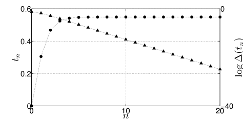
Figure 3: Escape time of RDE (18). Circle: $t_{n}$. Triangle: $\log\Delta(t_{n})$

Example 4.5

Consider the vector-valued RDE

$$\frac{dY}{dt}=\begin{bmatrix}0\\ -1\end{bmatrix}+\begin{bmatrix}2&-1\\ 3&-3\end{bmatrix}Y+Y-Y\begin{bmatrix}2&-1\end{bmatrix}Y$$ (19)

with the initial condition

$$Y_{0}=\begin{bmatrix}-0.5\\ -0.5\end{bmatrix}.$$

Fig. 4 shows the graph of $t_{n}$ and $\log(\Delta(t_{n}))$. Notice that in this case the scalar function $U(t)$ has a complicated form and it is not as easy to find its zeros as in Example 4.4.

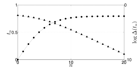
Figure 4: Escape time of RDE (19). Circle: $t_{n}$. Triangle: $\log\Delta(t_{n})$

Theorem 4.1 allows us to approximately compute the escape time of the deterministic RDEs for a fixed initial condition. On the other hand, to use Theorem 3.2 for the computation of the mean escape time of the switched RDE (9), we need the escape time of each of the deterministic RDEs (1) and (7) with arbitrary initial conditions. However, it is not feasible to apply the theorem to all the possible initial conditions. To fill in this gap, the following trivial lemma is useful.

Lemma 4.6

For any $Y_{0}\in\mathbb{R}^{(d-k)\times k}$ and $0\leq t<t_{A}(Y_{0})$ we have $t_{A}(Y(t;Y_{0}))=t_{A}(Y_{0})-t$.

Lemma 4.6 suggests that one instance of the computation of the escape time for a single initial condition allows us to find the escape time with various initial conditions. Specifically, finding the escape time for an initial state $Y_{0}$ by using Theorem 4.1 gives us the escape time for a family of initial states $\{Y(t;Y_{0})\}_{t=t_{0},t_{1},\dotsc}$. This observation leads us to Algorithm 1, which calculates the escape time for several many initial states efficiently.

Algorithm 1 Calculation of the escape time as a function of initial states

1:  Let $N$ be a positive integer. $D=\emptyset$.

2:  repeat

3:     Randomly choose an initial state $Y_{0}$.

4:     Compute the sequence $\{t_{n}\}_{n=0}^{N}$

5:     $D\leftarrow D\cup\{(Y(t_{N}-t_{n},Y_{0}),t_{n}\}_{n=0}^{N}$

6:  until Projection of $D$ into its first component becomes dense in the set of the initial states.

We illustrate the effectiveness of Algorithm 1 in the following example.

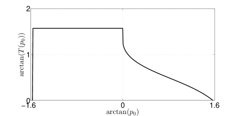
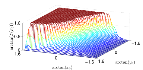
Figure 5: Escape time of the RDE (18)

Figure 6: Escape time of the RDE (19)

Example 4.7

We first apply Algorithm 1 to the scalar RDE (18). The algorithm gives the graph of the escape time as a function of initial states as in Fig. 6. Notice that, the real axis $\mathbb{R}$ (or the half real axis $[0,\infty)$) are rescaled to the closed interval $[-\pi/2,\pi/2]$ ($[0,\pi/2]$, respectively) with the arc-tangent function for the ease of presentation. The flatten part in the left half, where the graph takes the value $\pi/2$, means that the RDE never escapes in a finite time.

We then consider again the vector-valued Riccati differential equation (19). The associated matrix

$$A=\begin{bmatrix}-1&2&-1\\ 0&2&-1\\ -1&3&-3\end{bmatrix}$$

has the real and distinct eigenvalues $1.4605$, $-0.7609$, and $-2.6996$. Using Algorithm 1 we can draw the graph of the escape time as a function of initial states as in Fig. 6. Notice that the values are rescaled by the arc-tangent function as was did in Fig. 6.

4.2 A robustness result

Although Theorems 3.2 and 4.1 could allow us to approximately and numerically compute the mean escape time of the switched RDE (9), it is not clear if the computation is robust with respect to the computational error in Theorem 4.1 for the escape time of the deterministic RDEs. To provide an affirmative answer to this question, in this subsection we present a theorem showing that taking sufficiently many escape time using Algorithm 1 can lead to provide an accurate estimate of the mean escape time of the switched RDE (9).

Throughout this section, we will identify all the matrices $Y$ in $\mathbb{R}^{(d-k)\times k}$ with its image $\psi(Y)\in G_{0}^{k}(\mathbb{R}^{d})$ by the canonical chart. Since a Grassmann manifold is compact, the manifold is totally bounded. Therefore, the subset $G_{0}^{k}(\mathbb{R}^{d})$ is also totally bounded and hence admits a finite $\epsilon$-net for every $\epsilon>0$. This fact will allow us to discretize the state space with finitely many points.

In this subsection, in addition to Assumption 3.1, we also place the following technical assumption.

Assumption 4.8

The mean escape times $T_{A}$ and $T_{B}$ are uniformly continuous as functions from $G_{0}^{k}(\mathbb{R}^{d})$ to $\mathbb{R}$.

Under this assumption, the following theorem states that an accurate estimate of the mean escape time of the switched RDE (9) is possible by finitely many values of the escape time of deterministic RDEs (1) and (7).

Theorem 4.9

Let $\epsilon>0$ be arbitrary. Then, there exists a finite set $S=\{s_{1},\dotsc,s_{L}\}\subset G^{k}_{0}(\mathbb{R}^{d})$ and an invertible matrix $\Psi$ such that

$$\left\lVert\begin{bmatrix}T_{A}(S)\\ T_{B}(S)\end{bmatrix}-\Psi^{-1}\begin{bmatrix}g_{A}(S)\\ g_{B}(S)\end{bmatrix}\right\rVert_{\infty}<\epsilon.$$

To prove Theorem 4.9, we need the following lemma, which enables us to approximate the operators $M_{A}$ and $M_{B}$ by matrices.

Lemma 4.10

Let $\epsilon>0$ be arbitrary. Then, there exists a finite set $S=\{s_{1},\dotsc,s_{L}\}\subset G^{k}_{0}(\mathbb{R}^{d})$ and matrices $N_{A},N_{B}$ such that

$$\left\lVert(M_{A}T_{B})(S)-N_{A}(T_{B}(S))\right\rVert_{\infty} <\epsilon,$$

$$\left\lVert(M_{B}T_{A})(S)-N_{B}(T_{A}(S))\right\rVert_{\infty} <\epsilon$$

where, for a function $f\colon G^{k}_{0}(\mathbb{R}^{d})\to\mathbb{R}$, we write

$$f(S)=\begin{bmatrix}f(s_{1})\\ \vdots\\ f(s_{L})\end{bmatrix}\in\mathbb{R}^{L}.$$

Moreover, the matrices satisfy $\lVert N_{A}\rVert_{\infty},\lVert N_{B}\rVert_{\infty}\leq F(t_{0})$.

Proof 4

Let us first recall that the Grassmannian $G^{k}(\mathbb{R}^{d})$ can be equipped with the following distance; If $V_{1},V_{2}\in G^{n}(\mathbb{R}^{d})$ and $\pi_{1},\pi_{2}$ are orthogonal projections from $\mathbb{R}^{d}$ onto $V_{1},V_{2}$, respectively, then one can define a metric on $G^{n}(\mathbb{R}^{d})$ as $\rho(V_{1},V_{2})=\lVert\pi_{1}-\pi_{2}\rVert$.

Now, by symmetry, it is sufficient to prove only the first inequality in the lemma. Let $\epsilon>0$ be arbitrary. By Assumption 4.8 there exists $\delta>0$ such that if $\rho(P,P^{\prime})<\delta$, then $\lvert T_{A}(P)-T_{A}(P^{\prime})\rvert<\epsilon/2$. Then, we take a finite $\delta$-net $X=\{s_{1},\dotsc,s_{L}\}$ of $G^{k}_{0}(\mathbb{R}^{d})$. Let $q$ be a mapping on $G^{k}_{0}(\mathbb{R}^{d})$ that assigns to any $P$ one of $s_{\ell}$ within the distance of $\delta$.

Then $h>0$ and define the mapping $M_{A}^{\prime}T_{B}\colon G^{k}_{0}(\mathbb{R}^{d})\to\mathbb{R}$ by

$$(M^{\prime}_{A}T_{B})(P) =\sum_{n=0}^{\infty}T_{B}(P_{A}(nh;P))\xi_{A,n}(P),$$

$$\xi_{A,n}(P) =\int_{nh}^{(n+1)h}f(\tau)\chi_{[0,t_{A}(P))}(\tau)\,d\tau.$$

Since $L$ is finite we can take a sufficiently small $h>0$ such that, for every $\ell=1,\dotsc,L$,

$$\left|(M_{A}T_{B})(s_{\ell})-(M^{\prime}_{A}T_{B})(s_{\ell})\right|<\epsilon/2.$$ (20)

Let us fix such $h$. Then let us define $M_{A}^{\prime\prime}T_{B}\colon G^{k}_{0}(\mathbb{R}^{d})\to\mathbb{R}$ by $(M^{\prime\prime}_{A}T_{B})(P)=\sum_{n=0}^{\infty}T_{B}(q(P_{A}(nh;P)))\xi_{A,n}(P)$. Since $\rho(P,q(P))<\delta$ for every $P\in G^{k}_{0}(\mathbb{R}^{d})$, by the uniform continuity of $T_{B}$, for all $\ell=1,\dotsc,L$ it holds that $\lvert(M^{\prime}_{A}T_{B})(s_{\ell})-(M^{\prime\prime}_{A}T_{B})(s_{\ell})\rvert<\epsilon/2$. This inequality together with (20) implies

$$\lVert(M_{A}T_{B})(S)-(M^{\prime\prime}_{A}T_{B})(S)\rVert_{\infty}<\epsilon.$$

Now, since $(M^{\prime\prime}_{A}T_{B})(W_{k})$ is a linear combination of $T_{B}(s_{1})$, $\dotsc$, $T_{B}(s_{L})$ (notice that the image of $q$ is always one of $s_{\ell}$, $1\leq\ell\leq L$) there exists a matrix $N_{A}$ such that $(M^{\prime\prime}_{A}T_{B})(S)=N_{A}(T_{B}(S))$. This completes the proof of the first claim.

To prove the second claim, we just need to notice that the sum of the $\ell$th row of the matrix $N_{A}$ is equal to $\sum_{n=0}^{\infty}\xi_{A,n}(s_{\ell})=\int_{0}^{t_{A}(s_{\ell})}f(\tau)\,d\tau$, which is less always than or equal to $F(t_{0})$ by the assumption (10).

We can now prove Theorem 4.9.

Proof 5 (Theorem 4.9)

First let us apply Lemma 4.10 with the constant $F(t_{0})\epsilon$ to obtain a finite set $S=\{s_{1},\dotsc,s_{L}\}$ and matrices $N_{A},N_{B}$. Define

$$\Psi=\begin{bmatrix}I&-N_{A}\\ -N_{B}&I\end{bmatrix}.$$

By Lemmas 1.2 and 4.10, we can see that this matrix $\Psi$ is invertible and satisfy $\lVert\Psi^{-1}\rVert\leq 1/F(t_{0})$. Since

$$\begin{multlined}\begin{bmatrix}T_{A}(S)\\ T_{B}(S)\end{bmatrix}-\Psi^{-1}\begin{bmatrix}g_{A}(S)\\ g_{B}(S)\end{bmatrix}=\Psi^{-1}\begin{bmatrix}(M_{A}T_{B})(S)-N_{A}(T_{B}(S))\\ (M_{B}T_{A})(S)-N_{B}(T_{A}(S))\end{bmatrix}\end{multlined}\begin{bmatrix}T_{A}(S)\\ T_{B}(S)\end{bmatrix}-\Psi^{-1}\begin{bmatrix}g_{A}(S)\\ g_{B}(S)\end{bmatrix}=\Psi^{-1}\begin{bmatrix}(M_{A}T_{B})(S)-N_{A}(T_{B}(S))\\ (M_{B}T_{A})(S)-N_{B}(T_{A}(S))\end{bmatrix}$$

we have

$$\left\lVert\begin{bmatrix}T_{A}(S)\\ T_{B}(S)\end{bmatrix}-\Psi^{-1}\begin{bmatrix}g_{A}(S)\\ g_{B}(S)\end{bmatrix}\right\rVert<\lVert\Psi^{-1}\rVert(F(t_{0})\epsilon)\leq\epsilon,$$

as desired. This completes the proof of the theorem.

5 Conclusion

In this paper, we have investigated the computational aspects of the mean escape time of the switched RDEs subject to Poisson switching. We have first shown that, if the escape times of their subsystems are available, then we can find the mean escape time of the switched RDE as a convergent power series. We have then presented an approximation framework for numerically computing the escape time of RDEs as the limit of a convergent sequence, which can enhance the applicability of the characterization as a power series. Numerical simulations are presented to illustrate the obtained results.

References

- [1] M. A. Shayman, Phase portrait of the matrix Riccati equation, SIAM Journal on Control and Optimization 24 (1) (1986) 1–65.
- [2] T. Başar, Generalized Riccati equations in dynamics games, in: The Riccati Equation, Springer-Verlag, New York, 1989, pp. 293–333.
- [3] J. C. Doyle, K. Glover, P. P. Khargonekar, B. A. Francis, State space solutions to standard and control problems, IEEE Transactions on Automatic Control 34 (1989) 831–847.
- [4] K. W. Chang, Singular perturbations of a general boundary value problem, SIAM Journal on Mathematical Analysis 3 (3) (1972) 520–527.
- [5] G. Freiling, A survey of nonsymmetric Riccati equations, Linear Algebra and its Applications 351-352 (2002) 243–270.
- [6] G. N. Watson, A Treatise on the Theory of Bessel Functions, Cambridge University Press, 1995.
- [7] C. Martin, Finite escape time for Riccati differential equations, Systems & Control Letters 1 (2) (1981) 127–131.
- [8] T. Sasagawa, On the finite escape phenomena for matrix Riccati equations, IEEE Transactions on Automatic Control 27 (4) (1982) 977–979.
- [9] P. E. Crouch, M. Pavon, On the existence of solutions of the Riccati differential equation, Systems & Control Letters 9 (1987) 203–206.
- [10] B. F. Doolin, C. F. Martin, Introduction To Differential Geometry For Engineers, Marcel Dekker Inc, 1990.
- [11] W. M. Getz, D. H. Jacobson, Sufficiency conditions for finite escape times in systems of quadratic differential equations, J. Inst. Maths Applics 19 (1977) 377–383.
- [12] G. Freiling, G. Jank, A. Sarychev, Non-blow-up conditions for Riccati-type matrix differential and difference equations, Results in Mathematics 37 (2000) 84–103.
- [13] L. Zhang, E.-K. Boukas, J. Lam, Analysis and synthesis of Markov jump linear systems with time-varying delays and partially known transition probabilities, IEEE Transactions on Automatic Control 53 (10) (2008) 2458–2464.
- [14] X. Feng, K. Loparo, Y. Ji, H. Chizeck, Stochastic stability properties of jump linear systems, IEEE Transactions on Automatic Control 37 (1992) 38–53.
- [15] L. Zhang, J. Lam, Necessary and sufficient conditions for analysis and synthesis of Markov jump linear systems with incomplete transition descriptions, IEEE Transactions on Automatic Control 55 (7) (2010) 1695–1701.
- [16] P. Shi, F. Li, A survey on Markovian jump systems: Modeling and design, International Journal of Control, Automation and Systems 13 (1) (2015) 1–16.
- [17] Z. G. Wu, S. Dong, P. Shi, H. Su, T. Huang, R. Lu, Fuzzy-model-based nonfragile guaranteed cost control of nonlinear Markov jump systems, IEEE Transactions on Systems, Man, and Cybernetics: Systems 47 (8) (2017) 2388–2397.
- [18] L. Jin, Y. Yin, R. Loxton, Q. Lin, F. Liu, K. L. Teo, Optimal control of nonlinear Markov jump systems by control parametrisation technique, IET Control Theory and Applications (2022).
- [19] M. Zhang, P. Shi, L. Ma, J. Cai, H. Su, Quantized feedback control of fuzzy Markov jump systems, IEEE Transactions on Cybernetics 49 (9) (2019) 3375–3384.
- [20] M. Shen, J. H. Park, D. Ye, A Separated Approach to Control of Markov Jump Nonlinear Systems with General Transition Probabilities, IEEE Transactions on Cybernetics 46 (9) (2016) 2010–2018.
- [21] B. Hanlon, V. Tyuryaev, C. Martin, Stability of switched linear systems with Poisson switching, Communications in Information and Systems 11 (4) (2011) 307–326.
- [22] L. Jodar, E. Ponsoda, Non-autonomous Riccati-type matrix differential equations: existence interval, construction of continuous numerical solutions and error bounds, IMA journal of numerical analysis 15 (1) (1995) 61–74.
- [23] R. M. Corless, G. H. Gonnet, D. E. G. Hare, D. J. Jeffrey, D. E. Knuth, On the Lambert W function, Advances in Computational Mathematics 5 (1996) 329–359.