Computational protocol to evaluate electron-phonon interactions within density matrix perturbation theory

Abstract

We present a computational protocol, based on density matrix perturbation theory, to obtain non-adiabatic, frequency-dependent electron-phonon self-energies for molecules and solids. Our approach enables the evaluation of electron-phonon interaction using hybrid functionals, for spin-polarized systems, and the computational overhead to include dynamical and non-adiabatic terms in the evaluation of electron-phonon self-energies is negligible. We discuss results for molecules, as well as pristine and defective solids.

1 Introduction

The study of electron-phonon interaction in solids can be traced back to the early days of quantum mechanics¹, and it has been instrumental in explaining fundamental properties of solids, including conventional superconductivity². However, it was not until recent years that electron-phonon interaction was computed from first-principles^{3, 4, 5, 6, 7}, leading to non-phenomenological predictions of transport properties of solids⁸ and of electron-phonon renormalizations of band structures^{7, 9, 10, 11, 12}. While early studies relied on semi-empirical models^{13, 14, 15} to study electron-phonon interaction, modern investigations typically employ the frozen phonon (FPH) approach,^{16, 7} density functional perturbation theory (DFPT),^{4, 5, 10, 11, 17} or molecular dynamics (MD) simulations^{18, 19, 12}, with electron-electron and electron-ion interactions described at the level of density functional theory (DFT).²⁰

In two recent papers,^{10, 11} we combined first principles calculations of electron–electron and electron–phonon self-energies in molecules and solids, within the framework of density functional perturbation theory (DFPT). We developed an approach that enables the evaluation of electron–phonon coupling at the $G_{0}W_{0}$ level of theory for systems with hundreds of atoms, and the inclusion of non-adiabatic and temperature effects at no additional computational cost. We also computed¹² electron-phonon renormalizations of energy gaps by using the path-integral molecular dynamics (PIMD) methods to investigate anharmonic effects in crystalline and amorphous solids. The DFPT, FPH and MD-based methods are addressing different regimes and different problems; the use of DFPT and FPH are appropriate for systems whose atomic constituents all vibrate close to their equilibrium positions, although anharmonic effects have been included in some FPH calculations⁷. The assumption of close to equilibrium vibrations is however not required when applying PIMD, which thus has a wider applicability; for example it can be used to study amorphous materials, and molecules and solids exhibiting prominent anharmonic effects, e.g. molecular crystals^{21, 22} and several perovskites²³. However, the calculation of electron-phonon renormalizations using FPH and MD-based methods are carried out within the Allen-Heine-Cardona (AHC)^{24, 25} formalism, which neglects dynamical and non-adiabatic terms of the electron-phonon self-energies. These effects have been shown to be essential to describe electron-phonon interactions in numerous polar materials^{26, 27}, for example SiC. Perturbation-based methods, on the other hand, can accurately compute electron-phonon self-energies within and beyond the AHC formalism, thus including non-adiabatic and/or frequency-dependent effects into the self-energy. Another benefit of DFPT-based method is the ability to explicitly evaluate the electron-phonon coupling matrices which are useful quantities, for example, in the study of mobilities^{28, 29} and polaron hopping^{30, 31}.

Here we generalize the perturbation-based approach of Ref.10 and 11 to enable efficient calculations of electron-phonon interaction with hybrid functionals, by using density matrix perturbation theory (DMPT)^{32, 33} to compute phonons and electron-phonon coupling matrices. Our implementation takes advantage of the Lanczos algorithm³⁴, which enables the calculations of electron-phonon self-energies beyond the AHC approximation, at no extra cost.

DMPT has been used in the literature to compute excitation energies and absorption spectra in molecules and solids in conjunction with time-dependent density functional theory (TDDFT)^{35, 36}, and to solve the Bethe-Salpeter equation (BSE)^{37, 38, 33, 39, 40, 41}. In the latter case, DMPT has been applied to obtain the variation of single particle wavefunctions due to the perturbation of an electric field. However, DMPT is a general formalism that can be used to compute the response of a system to perturbations of any form, including perturbations caused by atomic displacements.

In this paper, we first derive a formalism for phonon calculations within DMPT, starting from the quantum Liouville equation in section 2; we then verify our results by comparing them with those of FPH and PIMD calculations in section 3. We then present calculations of electron-phonon interactions in small molecules (section 4), pristine (section 5) and defective diamond (section 6) using hybrid functionals and we conclude the paper in section 7 with a summary of our findings.

2 Methodology

Using Hartree atomic units ($\hbar=e=m_{e}=1$), we describe the electronic structure of a solid or molecule within Kohn-Sham (KS) density functional theory and we consider the quantum Liouville’s equation to describe perturbations acting on the system:

$$i\frac{\mathrm{d}}{\mathrm{d}t}\gamma(t)=[H^{\mathrm{KS}}(t),\gamma(t)],$$ (1)

where $[\cdot,\cdot]$ denotes a commutator, $H^{\mathrm{KS}}(t)$ is the Kohn-Sham Hamiltonian

$$H^{\mathrm{KS}}=K+V_{\mathrm{H}}+V_{\mathrm{ext}}+V_{\mathrm{xc}},$$ (2)

with $K$ the kinetic operator, $V_{\mathrm{H}}$ the Hartree potential, $V_{\mathrm{ext}}$ the external potential and $V_{\mathrm{xc}}$ the exchange-correlation potential. The KS Hamiltonian does not depend explicitly on time and depends implicitly on time through the time-dependent density matrix $\gamma$, that can be written in terms of Kohn-Sham single-particle orbitals $\psi_{n\sigma}$

$$\gamma({\mathbf{r}},{\mathbf{r}}^{\prime};t)=\sum_{\sigma}\sum_{n}^{N_{\mathrm{occ}}^{\sigma}}\psi_{n\sigma}({\mathbf{r}};t)\psi_{n\sigma}^{*}({\mathbf{r}}^{\prime};t),$$ (3)

where $\sigma$ is the spin polarization, $n$ is the band index and $N_{\mathrm{occ}}^{\sigma}$ is the number of occupied bands in the spin channel $\sigma$. Below we present calculations performed by sampling the Brillouin zone with only the $\Gamma$ point and hence omit labeling eigenstates with ${\mathbf{k}}$-points.

Given a time-dependent perturbation $\partial V_{\mathrm{ext}}(t)$ acting on the Hamiltonian, the first order change of the density matrix $\partial\gamma(t)$ satisfies the following equation,

$$i\frac{\mathrm{d}}{\mathrm{d}t}\partial\gamma(t)=\mathcal{L}\cdot\partial\gamma(t)+[\partial V_{\mathrm{ext}}(t),\gamma_{0}],$$ (4)

where $\mathcal{L}$ is the Liouville super-operator,

$$\mathcal{L}\cdot\partial\gamma(t)=[H^{\mathrm{KS}}_{0},\partial\gamma(t)]+[\partial V_{\mathrm{H}}[\partial\gamma(t)],\gamma_{0}]+[\partial V_{\mathrm{xc}}[\partial\gamma(t)],\gamma_{0}].$$ (5)

Here we use the notation $\partial$ to represent a change of potentials ($\partial V$), wavefunctions $\partial\psi$, charge densities $\partial\rho({\mathbf{r}})$ and density matrices $\partial\gamma({\mathbf{r}},{\mathbf{r}}^{\prime})$; $\gamma_{0}$ and $H^{\mathrm{KS}}_{0}$ are the density matrix and the Kohn-Sham Hamiltonian of the unperturbed system, respectively.

Taking the Fourier transform of Eq. (4), we rewrite it in the frequency domain,

$$(\omega-\mathcal{L})\cdot\partial\gamma(\omega)=[\partial V_{\mathrm{ext}}(\omega),\gamma_{0}].$$ (6)

In phonon calculations, we adopt the Born-Oppenheimer approximation⁴² and no retardation effects are included. Hence, we only need to solve Eq. (6) at $\omega=0$,

$$\mathcal{L}\cdot\partial\gamma=-[\partial V_{\mathrm{ext}},\gamma_{0}].$$ (7)

The equation above can be cast in the following form:

$$\left[\begin{array}[]{cc}\mathcal{D}+\mathcal{K}^{1e}-\mathcal{K}^{1d}&\mathcal{K}^{2e}-\mathcal{K}^{2d}\\ -\mathcal{K}^{2e}+\mathcal{K}^{2d}&-\mathcal{D}-\mathcal{K}^{1e}+\mathcal{K}^{1d}\end{array}\right]\left[\begin{array}[]{c}\mathcal{A}\\ \mathcal{B}\end{array}\right]=\left[\begin{array}[]{c}\left\{\left|-\mathcal{P}^{c}\partial V_{\mathrm{ext}}\psi_{n\sigma}\right\rangle:n=1,\cdots,N_{\mathrm{occ}}^{\sigma};\sigma=\uparrow,\,\downarrow\right\}\\ \left\{\left|\,\,\,\,\mathcal{P}^{c}\partial V_{\mathrm{ext}}\psi_{n\sigma}\right\rangle:n=1,\cdots,N_{\mathrm{occ}}^{\sigma};\sigma=\uparrow,\,\downarrow\right\}\end{array}\right]$$ (8)

where $\mathcal{P}^{c}$ is the projection operator onto the virtual bands; $\mathcal{K}^{1e}$, $\mathcal{K}^{2e}$, $\mathcal{K}^{1d}$, $\mathcal{K}^{2d}$, defined below in Eq. (12)–(13) and Eq. (15)–(18) are related to the variation of exchange-correlation potential $V_{\mathrm{xc}}$; the elements of the arrays $\mathcal{A}=\{a_{n\sigma}:n=1,\cdots,N_{\mathrm{occ}}^{\sigma};\sigma=\uparrow,\downarrow\}$ and $\mathcal{B}=\{b_{n\sigma}:n=1,\cdots,N_{\mathrm{occ}}^{\sigma};\sigma=\uparrow,\downarrow\}$ are variations of wavefunctions; the variation of the density matrix in terms of wavefunction variation is:

$$\partial\gamma=\sum_{\sigma}\sum_{n}^{N_{\mathrm{occ}}^{\sigma}}\big{[}\left|a_{n\sigma}\right\rangle\left\langle\psi_{n\sigma}\right|+\left|\psi_{n\sigma}\right\rangle\left\langle b_{n\sigma}\right|\big{]}$$ (9)

In phonon calculations, the external perturbation is static $\partial V_{\mathrm{ext}}(\omega=0)$, and Eq. (8) can be further simplified since $a_{n\sigma}=b_{n\sigma}=\partial\psi_{n\sigma}$ for static perturbations and Eq. (8) becomes:

$$\left[\mathcal{D}+\mathcal{K}^{1e}-\mathcal{K}^{1d}+\mathcal{K}^{2e}-\mathcal{K}^{2d}\right]\mathcal{A}=\left\{\left|-\mathcal{P}^{c}\partial V_{\mathrm{ext}}\psi_{n\sigma}\right\rangle:n=1,\cdots,N_{\mathrm{occ}}^{\sigma};\sigma=\uparrow,\,\downarrow\right\}.$$ (10)

Eq. (10) is a generalized Sternheimer equation,⁴³ where the operators on the left hand side are defined below.

$$\mathcal{D}\mathcal{A}=\left\{\mathcal{P}^{c}(H_{0}^{\mathrm{KS}}-\varepsilon_{n\sigma})\ket{a_{n\sigma}}:n=1,\cdots,N_{\mathrm{occ}}^{\sigma};\sigma=\uparrow,\,\downarrow\right\}.$$ (11)

When using LDA/GGA functionals, the $\mathcal{K}^{1e}$ and $\mathcal{K}^{2e}$ operators are:

$$\mathcal{K}^{1e}\mathcal{A}=\left\{\int\mathrm{d}\mathbf{r}^{\prime}\mathcal{P}^{c}(\mathbf{r},\mathbf{r}^{\prime})\psi_{n\sigma}(\mathbf{r}^{\prime})\sum_{\sigma^{\prime}}\sum_{n^{\prime}}^{N_{\mathrm{occ}}^{\sigma^{\prime}}}\int\mathrm{d}\mathbf{r}^{\prime\prime}f_{\mathrm{Hxc}}(\mathbf{r}^{\prime},\mathbf{r}^{\prime\prime})\psi_{n^{\prime}{\sigma^{\prime}}}^{*}(\mathbf{r}^{\prime\prime})a_{n^{\prime}{\sigma^{\prime}}}(\mathbf{r}^{\prime\prime}):n=1,\cdots,N_{\mathrm{occ}}^{\sigma};\sigma=\uparrow,\,\downarrow\right\},$$ (12)

$$\mathcal{K}^{2e}\mathcal{A}=\left\{\int\mathrm{d}\mathbf{r}^{\prime}\mathcal{P}^{c}(\mathbf{r},\mathbf{r}^{\prime})\psi_{n\sigma}(\mathbf{r}^{\prime})\sum_{\sigma^{\prime}}\sum_{n^{\prime}}^{N_{\mathrm{occ}}^{\sigma^{\prime}}}\int\mathrm{d}\mathbf{r}^{\prime\prime}f_{\mathrm{Hxc}}(\mathbf{r}^{\prime},\mathbf{r}^{\prime\prime})a_{n^{\prime}{\sigma^{\prime}}}^{*}(\mathbf{r}^{\prime\prime})\psi_{n^{\prime}{\sigma^{\prime}}}(\mathbf{r}^{\prime\prime}):n=1,\cdots,N_{\mathrm{occ}}^{\sigma};\sigma=\uparrow,\,\downarrow\right\},$$ (13)

where $f_{\mathrm{Hxc}}=v_{\mathrm{c}}+f_{\mathrm{xc}}$ is the sum of the bare Coulomb potential $v_{c}$ and the exchange-correlation kernel

$$f_{\mathrm{xc}}({\mathbf{r}},{\mathbf{r}}^{\prime})=\frac{\delta V_{\mathrm{xc}}({\mathbf{r}})}{\delta\rho({\mathbf{r}}^{\prime})}$$ (14)

with $\rho({\mathbf{r}})$ being the electron density.

When using hybrid functionals, the operators are:

$$\mathcal{K}^{1e}\mathcal{A}=\left\{\int\mathrm{d}\mathbf{r}^{\prime}\mathcal{P}^{c}(\mathbf{r},\mathbf{r}^{\prime})\psi_{n\sigma}(\mathbf{r}^{\prime})\sum_{\sigma^{\prime}}\sum_{n^{\prime}}^{N_{\mathrm{occ}}^{\sigma^{\prime}}}\int\mathrm{d}\mathbf{r}^{\prime\prime}f^{\mathrm{loc}}_{\mathrm{Hxc}}(\mathbf{r}^{\prime},\mathbf{r}^{\prime\prime})\psi_{n^{\prime}{\sigma^{\prime}}}^{*}(\mathbf{r}^{\prime\prime})a_{n^{\prime}{\sigma^{\prime}}}(\mathbf{r}^{\prime\prime}):n=1,\cdots,N_{\mathrm{occ}}^{\sigma};\sigma=\uparrow,\,\downarrow\right\},$$ (15)

$$\mathcal{K}^{2e}\mathcal{A}=\left\{\int\mathrm{d}\mathbf{r}^{\prime}\mathcal{P}^{c}(\mathbf{r},\mathbf{r}^{\prime})\psi_{n\sigma}(\mathbf{r}^{\prime})\sum_{\sigma^{\prime}}\sum_{n^{\prime}}^{N_{\mathrm{occ}}^{\sigma^{\prime}}}\int\mathrm{d}\mathbf{r}^{\prime\prime}f^{\mathrm{loc}}_{\mathrm{Hxc}}(\mathbf{r}^{\prime},\mathbf{r}^{\prime\prime})a_{n^{\prime}{\sigma^{\prime}}}^{*}(\mathbf{r}^{\prime\prime})\psi_{n^{\prime}{\sigma^{\prime}}}(\mathbf{r}^{\prime\prime}):n=1,\cdots,N_{\mathrm{occ}}^{\sigma};\sigma=\uparrow,\,\downarrow\right\},$$ (16)

$$\mathcal{K}^{1d}\mathcal{A}=\left\{\alpha\int\mathrm{d}{\mathbf{r}}^{\prime}\mathcal{P}^{c}({\mathbf{r}},{\mathbf{r}}^{\prime})\sum_{n^{\prime}}^{N_{\mathrm{occ}}^{\sigma}}a_{n^{\prime}\sigma}({\mathbf{r}}^{\prime})\int\mathrm{d}{\mathbf{r}}^{\prime\prime}v_{c}({\mathbf{r}}^{\prime},{\mathbf{r}}^{\prime\prime})\psi_{n^{\prime}\sigma}^{*}({\mathbf{r}}^{\prime\prime})\psi_{n\sigma}({\mathbf{r}}^{\prime\prime}):n=1,\cdots,N_{\mathrm{occ}}^{\sigma};\sigma=\uparrow,\,\downarrow\right\}$$ (17)

$$\mathcal{K}^{2d}\mathcal{A}=\left\{\alpha\int\mathrm{d}{\mathbf{r}}^{\prime}\mathcal{P}^{c}({\mathbf{r}},{\mathbf{r}}^{\prime})\sum_{n^{\prime}}^{N_{\mathrm{occ}}^{\sigma}}\psi_{n^{\prime}\sigma}({\mathbf{r}}^{\prime})\int\mathrm{d}{\mathbf{r}}^{\prime\prime}v_{c}({\mathbf{r}}^{\prime},{\mathbf{r}}^{\prime\prime})a_{n^{\prime}\sigma}^{*}({\mathbf{r}}^{\prime\prime})\psi_{n\sigma}({\mathbf{r}}^{\prime\prime}):n=1,\cdots,N_{\mathrm{occ}}^{\sigma};\sigma=\uparrow,\,\downarrow\right\}$$ (18)

where $f_{\mathrm{Hxc}}^{\mathrm{loc}}=v_{c}+f_{\mathrm{xc}}^{\mathrm{loc}}$ is the sum of the bare Coulomb potential and the local part of the exchange-correlation kernel

$$f^{\mathrm{loc}}_{\mathrm{xc}}({\mathbf{r}},{\mathbf{r}}^{\prime})=\frac{\delta V^{\mathrm{loc}}_{\mathrm{xc}}({\mathbf{r}})}{\delta\rho({\mathbf{r}}^{\prime})}$$ (19)

and the parameter $\alpha$ is the fraction of the Hartree-Fock exchange included in the definition of the hybrid functional. Note that the $\mathcal{K}^{1d}$ and the $\mathcal{K}^{2d}$ operators are zero for LDA/GGA functionals.

Once we have the solutions $a_{n\sigma}$ of the Liouville equation (Eq. (8) or Eq. (10)), i.e., the change of wavefunction $\partial\psi_{n\sigma}$, we can compute the change of the density matrix with Eq. (9); the change of density is then given by:

$$\partial\rho({\mathbf{r}})=\partial\gamma({\mathbf{r}},{\mathbf{r}})=\sum_{\sigma}\sum_{n}^{N_{\mathrm{occ}}^{\sigma}}\big{[}\partial\psi_{n\sigma}^{*}({\mathbf{r}})\psi_{n\sigma}({\mathbf{r}})+\psi_{n\sigma}^{*}({\mathbf{r}})\partial\psi_{n\sigma}({\mathbf{r}})\big{]}$$ (20)

and force constants are obtained as follows:

$$C_{I\alpha,J\beta}\propto\sum_{\sigma}\sum_{n}^{N_{\mathrm{occ}}^{\sigma}}\left\langle\partial_{I\alpha}\psi_{n\sigma}\left|\partial_{J\beta}V_{\mathrm{ext}}\right|\psi_{n\sigma}\right\rangle.$$ (21)

By diagonalizing the dynamical matrix,

$$\sum_{J\beta}\frac{1}{\sqrt{M_{I}M_{J}}}C_{I\alpha,J\beta}\xi_{J\beta,\nu}=\omega_{\nu}^{2}\xi_{I\alpha,\nu},$$ (22)

where $M_{I}$, $M_{J}$ are atomic masses, we obtain the frequency $\omega_{\nu}$ of mode $\nu$ and its polarization $\xi_{I\alpha,\nu}$.

To compute the electron-phonon coupling matrices in the Cartesian basis:

$$g_{mnI\alpha}^{\sigma}=\left\langle\psi_{m\sigma}\left|\partial_{I\alpha}V_{\mathrm{scf}}\right|\psi_{n\sigma}\right\rangle$$ (23)

or in the phonon mode basis:

$$g_{mn\nu}^{\sigma}=\sum_{I\alpha}\frac{\xi_{I\alpha,\nu}}{\sqrt{M_{I}}}g_{mnI\alpha}^{\sigma},$$ (24)

where $\xi_{I\alpha,\nu}$ is the $\nu$-th vibrational mode, we need to evaluate the change of the self-consistent (scf) potential $\partial V_{\mathrm{scf}}$. The scf potential is given by the sum of the Hartree potential $V_{\mathrm{H}}$, the local part of the exchange-correlation potential $V_{\mathrm{xc}}^{\mathrm{loc}}$ and the non-local Hatree-Fock exchange $V_{\mathrm{xc}}^{\mathrm{nl}}$. Thus, the change of the scf potential $\partial V_{\mathrm{scf}}\ket{\psi_{n\sigma}}$ is the sum of the following three terms:

$$\partial V_{\mathrm{H}}({\mathbf{r}})\ket{\psi_{n\sigma}({\mathbf{r}})}=\psi_{n\sigma}({\mathbf{r}})\int\mathrm{d}{\mathbf{r}}^{\prime}v_{c}({\mathbf{r}},{\mathbf{r}}^{\prime})\partial\rho({\mathbf{r}}^{\prime}),$$ (25)

$$\partial V_{\mathrm{xc}}^{\mathrm{loc}}({\mathbf{r}})\ket{\psi_{n\sigma}({\mathbf{r}})}=\psi_{n\sigma}({\mathbf{r}})\int\mathrm{d}{\mathbf{r}}^{\prime}f_{\mathrm{Hxc}}^{\mathrm{loc}}({\mathbf{r}},{\mathbf{r}}^{\prime})\partial\rho({\mathbf{r}}^{\prime}),$$ (26)

and

$$\partial V_{\mathrm{xc}}^{\mathrm{nl}}\ket{\psi_{n\sigma}}=-\alpha\sum_{n^{\prime}}^{N_{\mathrm{occ}}^{\sigma}}\int\mathrm{d}{\mathbf{r}}^{\prime}\left[\partial\psi_{n^{\prime}\sigma}^{*}({\mathbf{r}}^{\prime})\psi_{n^{\prime}\sigma}({\mathbf{r}})+\psi_{n^{\prime}\sigma}^{*}({\mathbf{r}}^{\prime})\partial\psi_{n^{\prime}\sigma}({\mathbf{r}})\right]v_{c}({\mathbf{r}},{\mathbf{r}}^{\prime})\psi_{n\sigma}({\mathbf{r}}^{\prime}).$$ (27)

The Fan-Migdal and Debye-Waller self-energies can then be computed as:

$$\braket{\psi_{n\sigma}}{\Sigma^{\mathrm{FM}}(\omega,T)}{\psi_{n\sigma}}=\sum_{m\nu}\left|g_{mn\nu}^{\sigma}\right|^{2}\left[\frac{b_{\nu}(T)+f_{m\sigma}(T)}{\omega-\varepsilon_{m\sigma}+\omega_{\nu}-i0^{+}}+\frac{b_{\nu}(T)+1-f_{m\sigma}(T)}{\omega-\varepsilon_{m\sigma}-\omega_{\nu}-i0^{+}}\right]$$ (28)

$$\braket{\psi_{n\sigma}}{\Sigma^{\mathrm{DW}}(T)}{\psi_{n\sigma}}=-\sum_{m\nu}\sum_{I\alpha J\beta}\frac{2b_{\nu}(T)+1}{\varepsilon_{n\sigma}-\varepsilon_{m\sigma}}\frac{1}{4\omega_{\nu}}\left[\frac{\xi_{I\alpha,\nu}\xi_{I\beta,\nu}}{M_{I}}+\frac{\xi_{J\alpha,\nu}\xi_{J\beta,\nu}}{M_{J}}\right]g^{\sigma}_{mnI\alpha}g^{\sigma}_{mn{J\beta}},$$ (29)

where $b_{\nu}$ is the occupation number of the frequency $\omega_{\nu}$ obeying the Bose-Einstein distribution and $f_{m\sigma}$ is the occupation number of the Kohn-Sham eigenvalues $\varepsilon_{m\sigma}$ obeying the Fermi-Dirac distribution. The Debye-Waller self-energy is derived within the rigid-ion approximation (RIA) ^{24, 44, 45}, which approximates second-order electron-phonon coupling matrices with first-order ones.

Using the frequency-dependent Fan-Migdal self-energy, the renormalized energy levels can be evaluated self-consistently,

$$\omega-\varepsilon_{{n\sigma}}=\braket{\psi_{n\sigma}}{\Sigma^{\mathrm{FM}}(\omega,T)+\Sigma^{\mathrm{DW}}(T)}{\psi_{n\sigma}}$$ (30)

with initial guess $\omega_{0}=\varepsilon_{n\sigma}$, and using the Lanczos³⁴ algorithm to evaluate the frequency-dependent Fan-Migdal self-energy (for a detailed derivation, see Ref. 10 and Ref. 11).

We refer to the FM self-energy in Eq. 28 as the non-adiabatic fully frequency-dependent (NA-FF) self-energy. If the frequency-dependence is considered within the adiabatic approximation, the self-energy is

$$\braket{\psi_{n\sigma}}{\Sigma^{\mathrm{FM}}_{\mathrm{A-FF}}(\omega,T)}{\psi_{n\sigma}}\simeq\sum_{m\nu}|g^{\sigma}_{mn\nu}|^{2}\frac{2b_{\nu}(T)+1}{\omega-\varepsilon_{m\sigma}}.$$ (31)

We refer to Eq. (31) as the adiabatic fully frequency-dependent (A-FF) self-energy.

In our formulation the evaluation of self-energies can be carried out simultaneously at multiple frequencies using the Lanczos algorithm; however, we introduce below approximations leading to frequency independent self-energies for comparison with results present in the literature, obtained e.g., with the Allen-Heine-Cardona (AHC) formalism^{24, 25}. In particular, we evaluate the FM self-energy by applying the so-called On-the-Mass-Shell (OMS) approximation, i.e., by setting $\omega=\varepsilon_{n\sigma}$ in the expressions of the A-FF and NA-FF self-energies. In the former case we obtain the adiabatic AHC (A-AHC)^{24, 25} approximation and in the latter case the non-adiabatic AHC (NA-AHC) approximation:

$$\braket{\psi_{n\sigma}}{\Sigma^{\mathrm{FM}}_{\mathrm{A-AHC}}(T)}{\psi_{n\sigma}}\simeq\sum_{m\nu}\left|g^{\sigma}_{mn\nu}\right|^{2}\frac{2b_{\nu}(T)+1}{\varepsilon_{{n\sigma}}-\varepsilon_{m\sigma}}$$ (32)

$$\braket{\psi_{n\sigma}}{\Sigma^{\mathrm{FM}}_{\mathrm{NA-AHC}}(T)}{\psi_{n\sigma}}=\sum_{m\nu}\left|g_{mn\nu}^{\sigma}\right|^{2}\left[\frac{b_{\nu}(T)+f_{m\sigma}(T)}{\varepsilon_{n\sigma}-\varepsilon_{m\sigma}+\omega_{\nu}-i0^{+}}+\frac{b_{\nu}+1-f_{m\sigma}}{\varepsilon_{n\sigma}-\varepsilon_{m\sigma}-\omega_{\nu}-i0^{+}}\right].$$ (33)

We summarize the various levels of approximations applied to evaluate the FM self-energy in Table 1; the corresponding DW self-energies are the same for all levels of approximation. Thus, we also use the acronyms A-AHC, NA-AHC, A-FF and NA-FF to denote the level of theory adopted for the total self-energy (FM + DW) and for the electron-phonon renormalization of fundamental gaps.

Table 1: A list of theoretical approximations used in this paper to compute the Fan-Migdal self-energy, where we specify whether the on-the-mass-shell (OMS) and the adiabatic approximation are adopted ($\checkmark$) or not adopted ($\times$)

Level of theory	OMS	Adiabatic	Equation
(A-)AHCa	$\checkmark$	$\checkmark$	(32)
NA-AHC	$\checkmark$	$\times$	(33)
A-FF	$\times$	$\checkmark$	(31)
NA-FF	$\times$	$\times$	(28)

• In the main text, we use AHC and A-AHC interchangeably.

3 Verification

To verify the implementation of the method described above in the WEST⁴⁶ package, we first computed the phonon frequencies of selected solids (diamond, silicon and silicon carbide) and the vibrational modes of selected molecules (H2, N2, H2O, CO2), and compared our results with those of the frozen phonon approach. In Table 2 and Table 3, we summarize our results obtained at the PBE0⁴⁷ level of theory and obtained by solving either the Liouville equation or by using the frozen phonon approach. The lattice constants used for diamond, silicon and silicon carbide are 3.635, 5.464 and 4.372 Å, respectively, and the cell used for molecules is a cube of edge $10.583$ Å. For verification purposes, we only computed the phonon modes at the $\Gamma$ point in the Brillouin zone of the solids. We used an energy cutoff of $60\,\mathrm{Ry}$ for the solids and $50\,\mathrm{Ry}$ for the molecules, and the SG15⁴⁸ ONCV⁴⁹ pseudopotentials for all solids and molecules.

Table 2 shows that the absolute difference of the phonon frequencies computed with the FPH approach and the method implemented here are small for silicon and silicon carbide, $0.19$ and $0.07\,\mathrm{cm^{-1}}$, respectively. The corresponding difference for diamond is larger, but still acceptable being below $5\,\mathrm{cm^{-1}}$. In Table 3, we compare the vibrational frequencies of H2, N2, H2O and CO2 molecules computed by solving the Liouville equation and applying the frozen-phonon approach. We found again that the differences are small for N2 and CO2 (below $1\,\mathrm{cm^{-1}}$), albeit slightly larger for H2 and H2O. The largest difference is found in the case of H2 ($17.30\,\mathrm{cm^{-1}}$), and this is most likely due to the numerical inaccuracy of the frozen-phonon approach.

Table 2: A comparison of selected phonon frequencies [$\mathrm{cm}^{-1}$] in diamond, silicon and silicon carbide computed in a primitive cell with the PBE0 functional by solving the Liouville’s equation or by using the frozen-phonon approach.

Solid	Liouville	Frozen-phonon	Absolute difference
diamond	2136.21	2131.48	4.73
silicon	737.47	737.28	0.19
silicon carbide	612.77	612.70	0.07

Table 3: A comparison of the vibrational modes [$\mathrm{cm}^{-1}$] of selected molecules obtained with the PBE0 functional and computed by solving the Liouville’s equation or by using the frozen-phonon approach. The symmetry of the mode is given in the second column.

Molecule	Symmetry	Liouville	Frozen-phonon	Absolute difference
H2	$a_{1}$	4421.48	4438.78	17.30
N2	$a_{1}$	2480.36	2480.36	0.00
H2O	$a_{1}$	1652.79	1658.76	5.97
H2O	$b_{2}$	3921.28	3936.57	15.29
H2O	$a_{1}$	4033.68	4048.58	11.90
CO2	$e_{1u}$	698.15	698.12	0.03
CO2	$a_{1g}$	1375.10	1375.18	0.08
CO2	$a_{1u}$	2419.08	2419.23	0.15

To verify our calculations of electron-phonon interactions, we carried out a detailed study of the renormalization of the HOMO-LUMO gaps ($E_{g}$) of the CO2, Si2H6, HCN, HF and N2 molecules, with the results for CO2 summarized in Table 4 and the rest in Table 5.

Table 4 summarizes the renormalizations to the $E_{g}$ of the CO2 molecule obtained within the A-AHC formalism, and using DFPT, FPH and path-integral molecular dynamics (PIMD)¹² at the LDA,⁵⁰ PBE,⁵¹ PBE0⁴⁷ and B3LYP^{52, 53, 54} levels of theory, respectively. With the LDA and PBE/GGA functionals, the solution of the Liouville equation yields the same results as the method proposed in Ref. 10 and Ref. 11, as expected. When solving the Liouville equation with the DFPT method, the rigid-ion approximation is adopted, however the latter approximation is not used in the frozen-phonon approach, leading to a slight difference between the frozen-phonon and Liouville results. In addition, we carried out calculations with the hybrid functionals, PBE0 and B3LYP, and compared our results with those of the frozen-phonon and PIMD approaches¹². The PIMD approach circumvents the rigid-ion approximation and also includes ionic anharmonic effects. Since the rigid-ion approximation is adopted and anharmonicity is not included in the Liouville approach, differences on the order of $\sim 30\,\mathrm{meV}$, relative to PIMD are considered as acceptable. We note that the computed renormalizations of the gap of CO2 reported in the literature,⁵⁵ $-680.7$ and $-716.2\,\mathrm{meV}$ with LDA⁵⁰ and PBE+TS⁵⁶ functionals, respectively, are significantly different from those obtained here. We also note that Ref.55 reports a result at the B3LYP level of theory, $-4091.6\,\mathrm{meV}$, which is one order of magnitude larger than the corresponding LDA and PBE+TS results, hence calling into question the numerical accuracy of the data. Such significant differences between our and the results of Ref. 55 probably stems from the different choices of basis functions, localized basis functions in Ref. 55 and plane-waves in this work.

In addition to CO2, we also computed the energy gap renormalizations of Si2H6, HCN, HF and N2 molecules with the B3LYP functional; these are shown in Table 5. For Si2H6 and HCN, the results computed with the Liouville’s equation and the FPH approach agree well, with small differences of $22$ and $5\,\mathrm{meV}$, respectively. The renormalization of HF is about $-20\,\mathrm{meV}$ with both the Liouville and FPH approaches, consistent with the result $-29.9\,\mathrm{meV}$ reported in literature. The Liouville and FPH methods both predict the renormalization of N2 to be close to zero, in agreement with Ref. 55.

In summary, we have verified our implementation of phonon and electron-phonon interaction by comparing results computed with the Liouville’s equation and those obtained with DFPT, FPH and PIMD methods. At the LDA/PBE level of theories, we obtain exactly the same results as with DFPT, as expected; at the hybrid functional level of theory, the results obtained with the Liouville’s equation are comparable with those of the FPH and PIMD methods, with reasonable differences compatible with the different approximations employed in the three different approaches.

Table 4: Electron-phonon renormalization energies [$\mathrm{meV}$] of HOMO, LUMO energy levels and the HOMO-LUMO gap in the CO2 molecule, computed by solving the Liouville’s equation, using density functional perturbation theory (DFPT), the frozen-phonon (FPH) approach and the path-integral molecular dynamics (PIMD) method. We compare results obtained with different functionals: LDA, PBE, PBE0 and the B3LYP functionals, and include results obtained in Ref. 55.

Method	Functional	HOMO Renorm.	LUMO Renorm.	Gap Renorm.
Liouville	LDA	64	-453	-517
DFPT	LDA	64	-453	-517
Liouville	PBE	65	-350	-415
DFPT	PBE	65	-350	-415
FPH	PBE	53	-325	-378
Liouville	PBE0	68	-69	-137
FPH	PBE0	55	-77	-132
PIMD	PBE0	59	-103	-162
Liouville	B3LYP	67	-107	-174
FPH	B3LYP	54	-89	-143
PIMD	B3LYP	58	-112	-170
Ref. 55	LDA	—	—	-680.7
	PBE+TS	—	—	-716.2
	B3LYP	—	—	-4091.6

Molecule	Liouville	FPH	Ref. 55
Si2H6	-117	-139	-1872.3
HCN	-19	-14	-171.4
HF	-18	-25	-29.9
N2	8	-6	8.7

Table 5: Electron-phonon renormalization energies [meV] of energy gap in Si2H6, HCN, HF and N2 molecules computed by solving the Liouville’s equation and using the frozon phonon (FPH) approach at the B3LYP level of theory.

4 Electron-phonon renormalization of energy gaps in small molecules

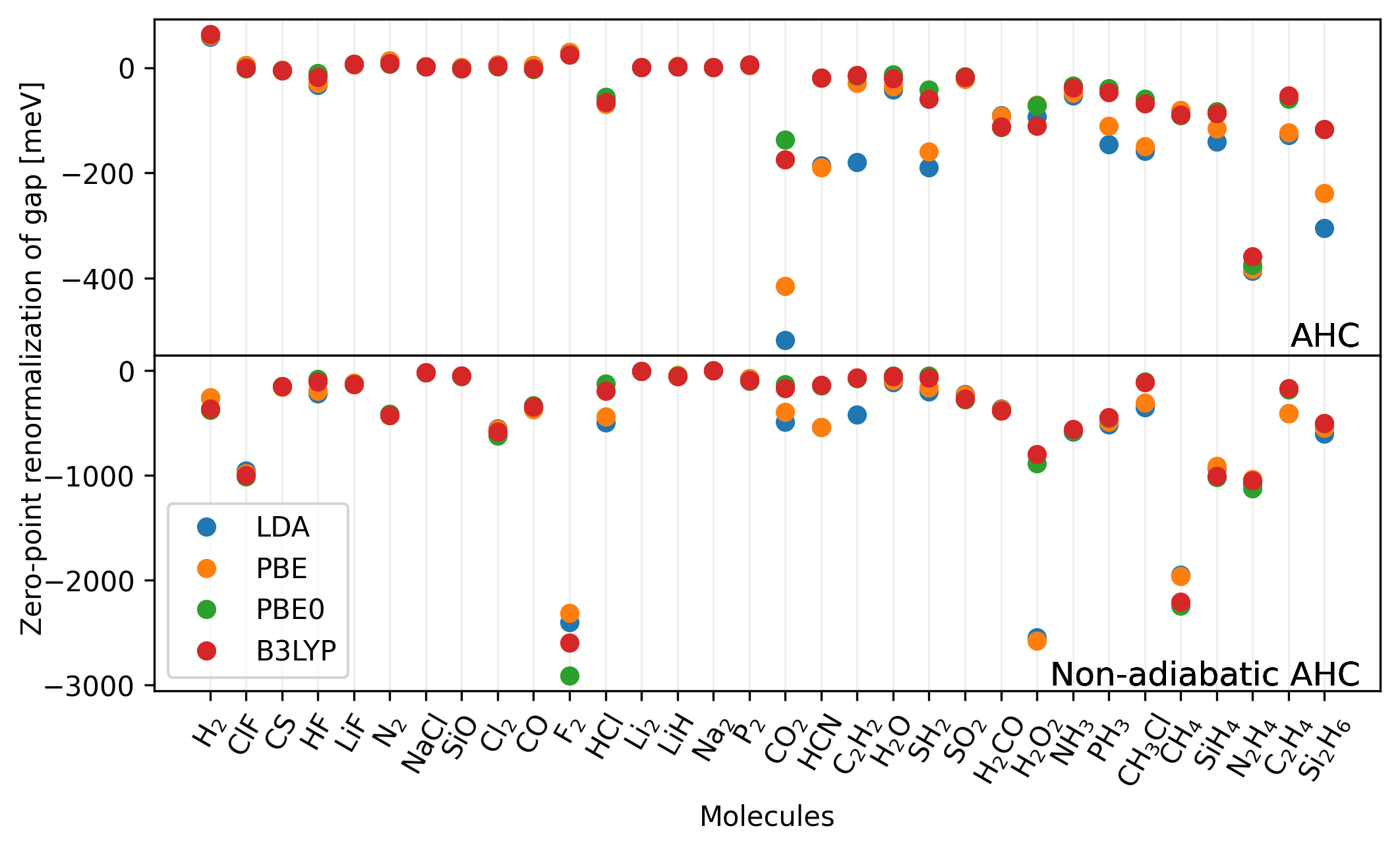
Figure 1: Computed zero-point renormalization energies of the HOMO-LUMO gaps of small molecules using the AHC (upper panel) and NA-AHC (lower panel) approximations (see Table 1. for the definition of the approximations). We used different functionals specified in the inset.

Having verified our implementation, we carried out a study of the renormalization of the HOMO-LUMO gap of molecules in the G2/97 test set⁵⁷ with LDA, PBE, PBE0 and B3LYP functionals. The results are summarized in Table 6 and Table 7, and are illustrated in Figure 1.

Table 6 summarizes the renormalizations computed with the A-AHC formalism. For most of the molecules, using hybrid functionals does not significantly change the gap renormalization relative to LDA or PBE results. For example, the energy gap renormalizations of the H2 molecule computed with LDA, PBE, PBE0 and B3LYP functionals are $58\,\mathrm{meV}$, $61\,\mathrm{meV}$, $63\,\mathrm{meV}$ and $63\,\mathrm{meV}$, respectively. However, hybrid functionals do reduce the magnitude of gap renormalization in several systems, and CO2 and CH3Cl are representative examples. In CO2 the renormalization is reduced from $-415\,\mathrm{meV}$ (PBE) to $-137\,\mathrm{meV}$ (PBE0) level of theory; in CH3Cl, it is reduced from $-149\,\mathrm{meV}$ (PBE) to $-59\,\mathrm{meV}$ (PBE0).

We report in Table 7 our results within the non-adiabatic AHC (NA-AHC) framework. The removal of the adiabatic approximation significantly influences the computed magnitude of the gap renormalization in most of the molecules, with some exceptions, e.g. CO2. For example, the H2 gap renormalization computed using PBE0 varies from $63\,\,\mathrm{meV}$ (AHC) to $-377\,\,\mathrm{meV}$ (NA-AHC). The most significant differences are found for the F2 and H2O2 molecules, where the gap renormalizations computed at the PBE0 level of theory are $25$ and $-72\,\mathrm{meV}$, respectively, within the AHC approach and $-2914$ and $-891\,\mathrm{meV}$, when using the non-adiabatic AHC method.

Table 6: HOMO-LUMO energy gaps of small molecules and their zero-point renormalization energy (ZPR) computed within the adiabatic Allen-Heine-Cardona (A-AHC) approximation. All gaps and ZPRs are in $\mathrm{eV}$. We compare results obtained with different energy functionals (LDA, PBE, PBE0 and B3LYP) and we also report ZPRs from Ref. 55 and, in few cases, Ref. 45

Molecule	LDA			PBE		PBE0		B3LYP
	gap	ZPR	Ref. 55	gap	ZPR	gap	ZPR	gap	ZPR	Ref. 55
H2	9.998	0.058	-0.0021	10.164	0.061	11.890	0.063	11.648	0.063	0.0036
			0.0579a
LiF	5.108	0.006	0.0331	4.723	0.006	7.014	0.007	6.601	0.007	0.0040
			0.0796a
N2	8.221	0.013	0.0118	8.319	0.013	11.707	0.007	11.179	0.008	0.0087
			0.0130a
CO	6.956	0.005	0.0065	7.074	0.004	10.055	-0.003	9.575	-0.002	0.0024
			0.0055a
ClF	3.194	0.004	0.0041	3.167	0.005	6.250	-0.002	5.629	-0.001	0.0025
CS	3.954	-0.004	-0.0042	4.042	-0.004	6.562	-0.006	6.199	-0.006	-0.0058
HF	8.681	-0.032	-0.0397	8.598	-0.030	11.302	-0.011	10.809	-0.018	-0.0299
NaCl	3.524	0.002	0.0001	3.225	0.002	5.069	0.002	4.577	0.002	0.0004
SiO	4.524	0.001	-0.0019	4.549	0.001	6.764	-0.002	6.368	-0.002	-0.0032
Cl2	2.899	0.006	0.0063	2.894	0.006	5.503	0.002	4.887	0.003	0.0060
F2	3.495	0.030	0.0369	3.370	0.029	7.840	0.025	6.917	0.025	0.0329
Li2	1.532	0.001	0.0006	1.524	0.001	2.582	0.001	2.343	0.001	0.0007
LiH	2.985	0.002	-0.0066	2.873	0.003	4.424	0.001	4.117	0.002	-0.0061
Na2	1.564	0.001	0.0002	1.521	0.001	2.495	0.000	2.264	0.001	0.0000
P2	3.649	0.005	0.0021	3.644	0.005	5.537	0.005	5.107	0.005	0.0037
CO2	8.075	-0.517	-0.6807	8.033	-0.415	10.159	-0.137	9.708	-0.174	-4.0916
HCN	7.878	-0.185	-0.1412	7.930	-0.190	10.186	-0.020	9.806	-0.019	-0.1714
H2O	6.272	-0.042	-0.0806	6.208	-0.036	8.511	-0.013	8.084	-0.020	-0.0524
SH2	5.212	-0.189	-0.0360	5.238	-0.160	6.942	-0.042	6.593	-0.059	-0.2117
SO2	3.457	-0.019	-0.0178	3.414	-0.021	6.087	-0.016	5.596	-0.018	-0.0186
H2CO	3.470	-0.091	-0.0876	3.589	-0.092	6.451	-0.114	5.993	-0.111	-0.1005
H2O2	5.028	-0.093	-0.1290	4.887	-0.071	7.780	-0.072	7.505	-0.110	-0.2254
NH3	5.395	-0.053	-0.0611	5.304	-0.048	7.205	-0.035	6.825	-0.038	-0.0333
PH3	5.999	-0.146	-0.0592	5.946	-0.110	7.388	-0.039	7.056	-0.047	-0.2017
C2H2	6.703	-0.179	-0.1901	6.712	-0.029	8.181	-0.016	7.835	-0.014	-0.2327
CH3Cl	6.232	-0.158	-0.1441	6.210	-0.149	8.042	-0.059	7.691	-0.068	-0.1141
CH4	8.799	-0.084	-0.1147	8.820	-0.081	10.647	-0.091	10.320	-0.090	-0.0947
SiH4	7.727	-0.141	-0.6149	7.772	-0.115	9.440	-0.083	9.187	-0.086	-0.2027
N2H4	4.892	-0.386	-0.1169	4.866	-0.383	6.736	-0.375	6.426	-0.359	-0.0793
C2H4	5.654	-0.129	-0.1358	5.673	-0.123	7.592	-0.059	7.224	-0.053	-0.1194
Si2H6	6.364	-0.305	-0.5880	6.386	-0.238	7.874	-0.117	7.609	-0.117	-1.8723

• Ref. 45

Table 7: HOMO-LUMO gaps of small molecules and their zero-point renormalization energies (ZPR) computed within the non-adiabatic Allen-Heine-Cardona (NA-AHC) approximation. All gaps and ZPRs are in $\mathrm{eV}$. We compare results obtained with different energy functionals (LDA, PBE, PBE0, B3LYP).

Molecule	LDA		PBE		PBE0		B3LYP
	gap	ZPR	gap	ZPR	gap	ZPR	gap	ZPR
H2	9.998	-0.260	10.164	-0.263	11.890	-0.377	11.648	-0.366
LiF	5.108	-0.123	4.723	-0.122	7.014	-0.134	6.601	-0.134
N2	8.221	-0.418	8.319	-0.432	11.707	-0.418	11.179	-0.428
CO	6.956	-0.361	7.074	-0.373	10.055	-0.338	9.575	-0.346
ClF	3.194	-0.959	3.167	-0.985	6.250	-1.011	5.629	-1.000
CS	3.954	-0.151	4.042	-0.156	6.562	-0.155	6.199	-0.154
HF	8.681	-0.225	8.598	-0.194	11.302	-0.083	10.809	-0.111
NaCl	3.524	-0.021	3.225	-0.022	5.069	-0.022	4.577	-0.022
SiO	4.524	-0.052	4.549	-0.054	6.764	-0.056	6.368	-0.055
Cl2	2.899	-0.557	2.894	-0.560	5.503	-0.622	4.887	-0.589
F2	3.495	-2.405	3.370	-2.317	7.840	-2.914	6.917	-2.600
HCl	6.768	-0.501	6.784	-0.440	8.858	-0.128	8.417	-0.195
Li2	1.532	-0.007	1.524	-0.008	2.582	-0.010	2.343	-0.010
LiH	2.985	-0.049	2.873	-0.045	4.424	-0.055	4.117	-0.058
Na2	1.564	-0.002	1.521	-0.002	2.495	-0.002	2.264	-0.002
P2	3.649	-0.077	3.644	-0.079	5.537	-0.100	5.107	-0.096
CO2	8.075	-0.495	8.033	-0.398	10.159	-0.136	9.708	-0.174
HCN	7.878	-0.543	7.930	-0.541	10.186	-0.147	9.806	-0.138
H2O	6.272	-0.114	6.208	-0.095	8.511	-0.050	8.084	-0.061
SH2	5.212	-0.203	5.238	-0.166	6.942	-0.050	6.593	-0.069
SO2	3.457	-0.231	3.414	-0.234	6.087	-0.281	5.596	-0.274
H2CO	3.470	-0.364	3.589	-0.376	6.451	-0.386	5.993	-0.382
H2O2	5.028	-2.549	4.887	-2.582	7.780	-0.891	7.505	-0.799
NH3	5.395	-0.590	5.304	-0.566	7.205	-0.578	6.825	-0.562
PH3	5.999	-0.516	5.946	-0.493	7.388	-0.453	7.056	-0.450
C2H2	6.703	-0.420	6.712	-0.074	8.181	-0.080	7.835	-0.073
CH3Cl	6.232	-0.351	6.210	-0.307	8.042	-0.112	7.691	-0.116
CH4	8.799	-1.950	8.820	-1.961	10.647	-2.245	10.320	-2.210
SiH4	7.727	-0.931	7.772	-0.916	9.440	-1.019	9.187	-1.007
N2H4	4.892	-1.082	4.866	-1.038	6.736	-1.129	6.426	-1.050
C2H4	5.654	-0.408	5.673	-0.411	7.592	-0.184	7.224	-0.173
Si2H6	6.364	-0.607	6.386	-0.551	7.874	-0.506	7.609	-0.507

We emphasize that neither the AHC nor the non-adiabtic AHC formalism correctly describes the self-energies in the full energy range, and thus we suggest that the frequency-dependent self-energies should always be computed.

5 Electron-phonon renormalization of the energy gap of diamond

We computed the electron-phonon renormalization of the energy gap in diamond within the AHC formalism, and by computing the NA-FF self-energies self-consistently (see Table 1 and Eq. (30)). The calculations for diamond were carried out in a $3\times 3\times 3$ supercell.

In Figure 2, we present the temperature-dependent indirect gap renormalization computed with the PBE, PBE0 and dielectric dependent hybrid (DDH) functionals,^{58, 59} where the fraction of exact exchange (0.18) in DDH is chosen to be the inverse of the dielectric constant of diamond (5.61).⁵⁸ Within the same level of approximation, e.g., the AHC formalism (circles in the plot), the PBE, PBE0 and DDH results are almost the same for temperatures lower than $400\,\mathrm{K}$, but their difference increases at higher temperatures. With the same functional, e.g., the PBE0 functional (orange lines in the plot), the results obtained with the fully frequency-dependent non-adiabatic self-energies are lower than those obtained with the AHC formalism. In general, the use of the hybrid functional does not significantly modify the trend of the ZPRs computed at the PBE level, as a function of temperature.

In Figure 2, we also report the renormalization of the indirect gap of diamond obtained with the frozen phonon approach and the PBE0 functional. The results obtained with the FPH (purple line) approach and the Liouville equation (orange lines in the plot) are essentiallyy the same below $300\,\mathrm{K}$, but they differ as T is increased. The difference between the AHC/NA-FF and FPH approaches is always smaller than $10\,\mathrm{meV}$ at all temperatures, and it is reasonable considering that the FPH approach does not adopt the rigid-ion approximationg, which is instead used within the AHC and NA-FF approaches.

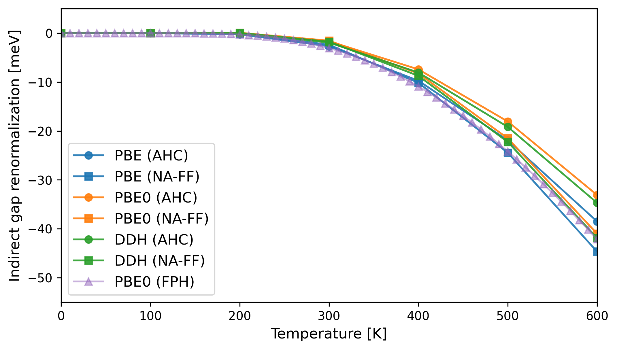
Figure 2: The electron-phonon renormalization energy of the indirect band gap of diamond computed by solving the Liouville equation and with different approximations to the self-energy, as defined in Table 1. The results obtained with the frozen phonon (FPH) approach and the PBE0 functional are also reported for comparison. The renormalization energy at zero temperature has been shifted to zero.

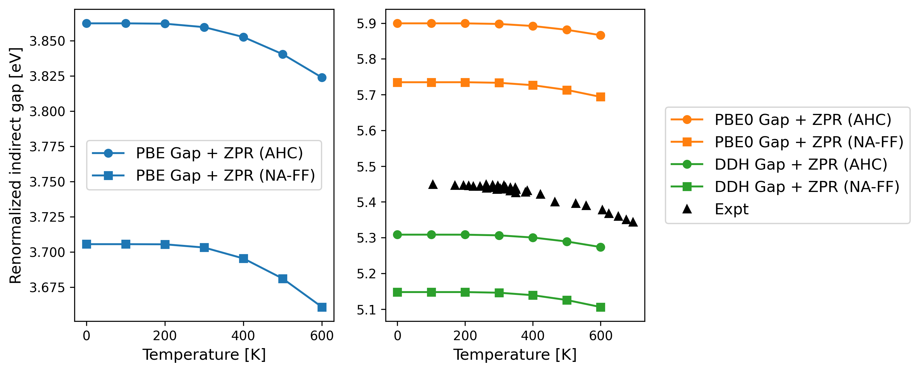
Figure 3: The electron-phonon renormalized indirect energy gap in diamond computed with the PBE and PBE0 functionals compared to experimental measurements.⁶⁰ We show calculations performed with different approximations, as defined in Table 1.

Table 8: The temperature-dependent zero-point renormalization energy (ZPR) and renormalized indirect energy gap (Gap+ZPR) computed with the PBE, PBE0 and DDH functionals, using different levels of approximations, as defined in Table 1. The energy gaps computed at the PBE, PBE0 and DDH level of theory, without electron-phonon interaction, are $4.144$, $6.189$ and $5.597\,\mathrm{eV}$ respectively. All energies are reported in eV.

	Functional	Method	Temperature [K]
			0	100	200	300	400	500	600
ZPR	PBE	AHC	-0.281	-0.281	-0.282	-0.284	-0.291	-0.303	-0.320
		NA-FF	-0.438	-0.438	-0.438	-0.441	-0.448	-0.463	-0.483
	PBE0	AHC	-0.290	-0.290	-0.290	-0.291	-0.297	-0.308	-0.323
		NA-FF	-0.454	-0.454	-0.454	-0.456	-0.463	-0.476	-0.495
	DDH	AHC	-0.289	-0.289	-0.289	-0.291	-0.297	-0.308	-0.324
		NA-FF	-0.450	-0.450	-0.450	-0.451	-0.458	-0.472	-0.492
Gap+ZPR	PBE	AHC	3.862	3.862	3.862	3.860	3.853	3.840	3.824
		NA-FF	3.705	3.705	3.705	3.703	3.695	3.681	3.661
	PBE0	AHC	5.899	5.899	5.899	5.898	5.892	5.881	5.866
		NA-FF	5.735	5.735	5.735	5.733	5.726	5.713	5.694
	DDH	AHC	5.308	5.308	5.308	5.306	5.300	5.289	5.274
		NA-FF	5.148	5.148	5.148	5.146	5.139	5.125	5.106

A comparison of the computed and measured renormalized energy gap of diamond is given in Figure 3 and Table 8. Although the PBE0 and DDH hybrid functionals yield a similar trend as PBE for the electron-phonon renormalization as a function of temperature, the renormalized gap are noticeably improved compared to experiments when using hybrid functionals. The indirect energy gap of diamond computed with PBE, PBE0 and DDH without electron-phonon renormalizaiton are $4.144$, $6.189$, and $5.597\,\mathrm{eV}$, respectively, and the experimental indirect gap measured at approximately $100\,\mathrm{K}$ is $5.45\,\mathrm{eV}$.⁶⁰. By including electron-phonon renormalizaiton, we can see that the results computed at the PBE0 level of theory agree relatively well with the experimental measurements (see Figure 3 and Table 8). The renormalized indirect gap computed with the PBE0 functional at $100\,\mathrm{K}$ is $5.899\,\mathrm{eV}$ when the AHC formalism is used, and it is $5.735\,\mathrm{eV}$ when the NA-FF self-energies are used. The renormalized indirect gaps computed with the DDH functional at $100\,\mathrm{K}$ are $5.308$ (AHC) and $5.148\,\mathrm{eV}$ (NA-FF). As expected, the DDH results are closer to experimental measurements compared with those of the PBE0 functional, since the fraction of exact exchange is chosen according to the system specific dielectric constant. Overall we find that computing electron-phonon interactions at the hybrid level of theory is a promising protocol to obtain quantitative results, comparable to experiments.

6 Application to spin defects in diamond

Spin defects have been extensively studied due to their potential applications in quantum technologies.^{61, 62, 63, 64} To accurately predict the electronic structures of spin defects, we computed their electronic properties using electron-phonon renormalizations and we considered a single Boron defect and the $\mathrm{NV}^{-}$ center shown in Figure 4. The calculations were carried out in a $2\times 2\times 2$ cubic cell (63 atoms for $\mathrm{NV}^{-}$ center and 64 atoms for single Boron defect).

In Table 9 and Table 10, we report the electronic energy levels and zero-point renormalization for both defects obtained with the PBE, PBE0 and DDH functionals. We found that electron-phonon interactions weakly affect the energy levels of the $\mathrm{NV}^{-}$ center, which exhibit localized wavefunctions; they are instead more significant for the single Boron defect with delocalized wavefunctions. In the $\mathrm{NV}^{-}$ center, the ZPR of the LUMO computed with the PBE functional is only $-35\,\mathrm{meV}$ and that of the HOMO is negligible. In addition, the hybrid functionals PBE0 and DDH yield results similar to PBE. For the boron defect, with PBE (DDH) functional, the ZPRs of HOMO and LUMO are $111\,\mathrm{meV}$ (121) and $126\,\mathrm{meV}$ (241), respectively.

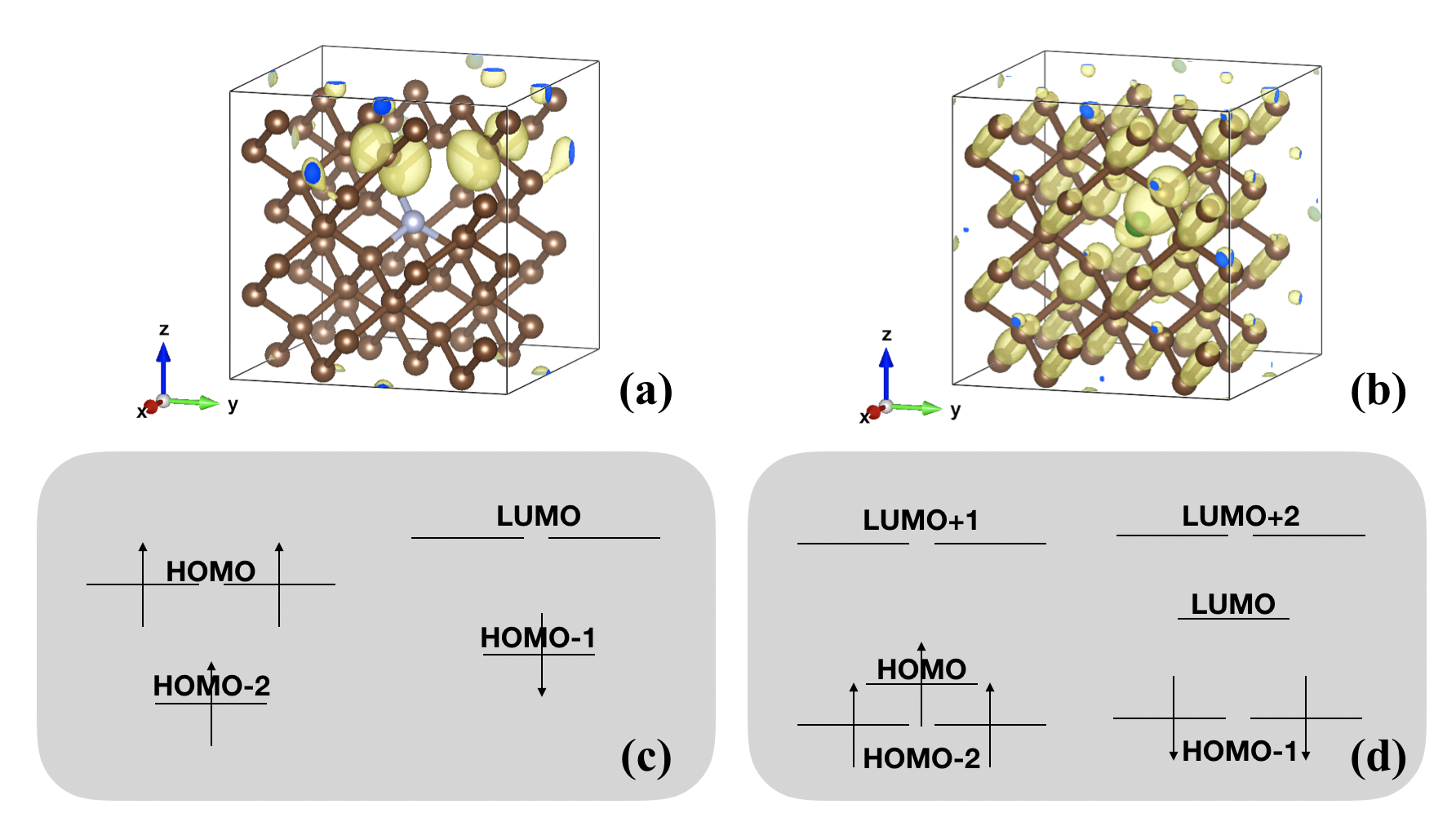
Figure 4: (a) The localized occupied state introduced by the nitrogen vacancy defect and (b) the delocalized unoccupied state introduced by the single boron vacancy defect. The wavefunctions are computed with the dielectric dependent hybrid functional. (c) and (d) illustrate the level ordering within the energy gap of diamond.

Table 9: Computed energy levels ($\mathrm{eV}$) and their zero-point renormalizations ($\mathrm{eV}$) in $\mathrm{NV}^{-}$ center. Energy levels are referred to the HOMO energy level, and the labels of energy levels are given in Figure 4(c).

	PBE		PBE0		DDH
	Level	ZPR	Level	ZPR	Level	ZPR
LUMO	1.359	-0.035	3.593	-0.033	2.948	-0.033
HOMO	0.000	0.001	0.000	0.012	0.000	0.009
HOMO-1	-0.411	0.012	-0.059	0.004	-0.189	0.008
HOMO-2	-0.924	0.038	-0.942	0.057	-0.952	0.052

Table 10: Computed energy levels ($\mathrm{eV}$) and their zero-point renormalizations ($\mathrm{eV}$) in the boron defect. Energy levels are referred to the HOMO energy level, and the labels of energy levels are given in Figure 4(d).

	PBE		PBE0		DDH
	Level	ZPR	Level	ZPR	Level	ZPR
LUMO+2	4.061	-0.359	6.109	-0.367	5.517	-0.365
LUMO+1	4.041	-0.361	6.090	-0.368	5.498	-0.367
LUMO	0.137	0.126	1.389	0.285	1.027	0.241
HOMO	0.000	0.111	0.000	0.126	0.000	0.121
HOMO-1	-0.278	0.087	-0.319	0.054	-0.308	0.062
HOMO-2	-0.287	0.089	-0.327	0.104	-0.316	0.100

7 Conclusions

In this paper, we computed phonon frequencies and electron-phonon interaction at the level of hybrid density functional theory by using density matrix perturbation theory and by solving the Liouville equation. Using this approach, we obtained phonon frequencies and energy gap renormalizations for molecules and solids by evaluating the non-adiabatic full frequency-dependent electron-phonon self-energies, thus circumventing the static and adiabatic approximations adopted in the AHC formalism, at no extra computational cost. We investigated the electronic properties of small molecules using LDA, PBE, B3LYP and PBE0 functionals. We also carried out calculations of the electronic structure of diamond with the PBE, PBE0 and DDH functionals, and found that the hybrid funtionals PBE0/DDH noticeably improve the renormalized energy gap compared to experimental measurements. In addition, we studied the electron-phonon renormalizations of defects in diamond, and we concluded that electron-phonon effects are essential to fully understand the electronic structures of defects, especially those with relatively delocalized states.

In conclusion, computing electron-phonon interactions at the hybrid functional level of theory is a promising protocol to accurately describe the electronic structure of molecules and solids, and density matrix perturbation theory is a general technique that allows one to do so in an efficient and accurate manner, by evaluating non adiabatic and full frequency dependent electron-phonon self-energies.

This work was supported by the Midwest Integrated Center for Computational Materials (MICCoM) as part of the Computational Materials Sciences Program funded by the U.S. Department of Energy. This research used resources of the National Energy Research Scientific Computing Center (NERSC), a DOE Office of Science User Facility supported by the Office of Science of the U.S. Department of Energy under Contract No. DE-AC02-05CH11231, resources of the Argonne Leadership Computing Facility, which is a DOE Office of Science User Facility supported under Contract DE-AC02-06CH11357, and resources of the University of Chicago Research Computing Center.

References

- Bloch 1929 Bloch, F. Über die quantenmechanik der elektronen in kristallgittern. Z. Phys. 1929, 52, 555–600
- Bardeen et al. 1957 Bardeen, J.; Cooper, L. N.; Schrieffer, J. R. Microscopic Theory of Superconductivity. Phys. Rev. 1957, 106, 162–164
- Giannozzi et al. 1991 Giannozzi, P.; de Gironcoli, S.; Pavone, P.; Baroni, S. Ab initiocalculation of phonon dispersions in semiconductors. Phys. Rev. B 1991, 43, 7231–7242
- Baroni et al. 2001 Baroni, S.; de Gironcoli, S.; Corso, A. D.; Giannozzi, P. Phonons and related crystal properties from density-functional perturbation theory. Rev. Mod. Phys. 2001, 73, 515–562
- Giustino et al. 2007 Giustino, F.; Cohen, M. L.; Louie, S. G. Electron-phonon interaction using Wannier functions. Phys. Rev. B 2007, 76, 165108
- Giustino 2017 Giustino, F. Electron-phonon interactions from first principles. Rev. Mod. Phys. 2017, 89, 015003
- Antonius et al. 2014 Antonius, G.; Poncé, S.; Boulanger, P.; Côté, M.; Gonze, X. Many-Body Effects on the Zero-Point Renormalization of the Band Structure. Phys. Rev. Lett. 2014, 112, 215501
- Poncé et al. 2018 Poncé, S.; Margine, E. R.; Giustino, F. Towards predictive many-body calculations of phonon-limited carrier mobilities in semiconductors. Physical Review B 2018, 97, 121201
- Poncé et al. 2015 Poncé, S.; Gillet, Y.; Janssen, J. L.; Marini, A.; Verstraete, M.; Gonze, X. Temperature dependence of the electronic structure of semiconductors and insulators. J. Chem. Phys. 2015, 143, 102813
- McAvoy et al. 2018 McAvoy, R. L.; Govoni, M.; Galli, G. Coupling First-Principles Calculations of Electron–Electron and Electron–Phonon Scattering, and Applications to Carbon-Based Nanostructures. J. Chem. Theory Comput. 2018, 14, 6269–6275
- Yang et al. 2021 Yang, H.; Govoni, M.; Kundu, A.; Galli, G. Combined First-Principles Calculations of Electron–Electron and Electron–Phonon Self-Energies in Condensed Systems. Journal of Chemical Theory and Computation 2021, 17, 7468–7476
- Kundu et al. 2021 Kundu, A.; Govoni, M.; Yang, H.; Ceriotti, M.; Gygi, F.; Galli, G. Quantum vibronic effects on the electronic properties of solid and molecular carbon. Phys. Rev. Materials 2021, 5, L070801
- Fan 1950 Fan, H. Y. Temperature Dependence of the Energy Gap in Monatomic Semiconductors. Phys. Rev. 1950, 78, 808–809
- Fan 1951 Fan, H. Y. Temperature dependence of the energy gap in semiconductors. Phys. Rev. 1951, 82, 900
- Fröhlich et al. 1950 Fröhlich, H.; Pelzer, H.; Zienau, S. XX. Properties of slow electrons in polar materials. London, Edinburgh Dublin Philos. Mag. J. Sci. 1950, 41, 221–242
- Monserrat 2018 Monserrat, B. Electron–phonon coupling from finite differences. J. Phys.: Condens. Matter 2018, 30, 083001
- Engel et al. 2022 Engel, M.; Miranda, H.; Chaput, L.; Togo, A.; Verdi, C.; Marsman, M.; Kresse, G. Zero-point Renormalization of the Band Gap of Semiconductors and Insulators Using the PAW Method. 2022; https://arxiv.org/abs/2205.04265
- Karsai et al. 2018 Karsai, F.; Engel, M.; Flage-Larsen, E.; Kresse, G. Electron–phonon coupling in semiconductors within the approximation. New J. Phys. 2018, 20, 123008
- Monserrat and Needs 2014 Monserrat, B.; Needs, R. Comparing electron-phonon coupling strength in diamond, silicon, and silicon carbide: First-principles study. Phys. Rev. B 2014, 89, 214304
- Kohn and Sham 1965 Kohn, W.; Sham, L. J. Self-Consistent Equations Including Exchange and Correlation Effects. Phys. Rev. 1965, 140, A1133–A1138
- Monserrat et al. 2015 Monserrat, B.; Engel, E. A.; Needs, R. J. Giant electron-phonon interactions in molecular crystals and the importance of nonquadratic coupling. Physical Review B 2015, 92, 140302
- Kundu et al. 2022 Kundu, A.; Govoni, M.; Galli, G. Unpublished. 2022,
- Knoop et al. 2020 Knoop, F.; Purcell, T. A.; Scheffler, M.; Carbogno, C. Anharmonicity measure for materials. Physical Review Materials 2020, 4, 083809
- Allen and Heine 1976 Allen, P. B.; Heine, V. Theory of the temperature dependence of electronic band structures. J. Phys. C: Solid State Phys. 1976, 9, 2305
- Allen and Cardona 1981 Allen, P. B.; Cardona, M. Theory of the temperature dependence of the direct gap of germanium. Phys. Rev. B 1981, 23, 1495
- Antonius et al. 2015 Antonius, G.; Poncé, S.; Lantagne-Hurtubise, E.; Auclair, G.; Gonze, X.; Côté, M. Dynamical and anharmonic effects on the electron-phonon coupling and the zero-point renormalization of the electronic structure. Phys. Rev. B 2015, 92, 085137
- Miglio et al. 2020 Miglio, A.; Brousseau-Couture, V.; Godbout, E.; Antonius, G.; Chan, Y.-H.; Louie, S. G.; Côté, M.; Giantomassi, M.; Gonze, X. Predominance of non-adiabatic effects in zero-point renormalization of the electronic band gap. npj Comput. Mater. 2020, 6, 1–8
- Li 2015 Li, W. Electrical transport limited by electron-phonon coupling from Boltzmann transport equation: An ab initio study of Si, Al, and MoS 2. Physical Review B 2015, 92, 075405
- Poncé et al. 2018 Poncé, S.; Margine, E. R.; Giustino, F. Towards predictive many-body calculations of phonon-limited carrier mobilities in semiconductors. Physical Review B 2018, 97, 121201
- Sio et al. 2019 Sio, W. H.; Verdi, C.; Poncé, S.; Giustino, F. Ab initio theory of polarons: Formalism and applications. Physical Review B 2019, 99, 235139
- Sio et al. 2019 Sio, W. H.; Verdi, C.; Poncé, S.; Giustino, F. Polarons from first principles, without supercells. Physical Review Letters 2019, 122, 246403
- Walker et al. 2006 Walker, B.; Saitta, A. M.; Gebauer, R.; Baroni, S. Efficient Approach to Time-Dependent Density-Functional Perturbation Theory for Optical Spectroscopy. Phys. Rev. Lett. 2006, 96, 113001
- Rocca et al. 2010 Rocca, D.; Lu, D.; Galli, G. Ab initio calculations of optical absorption spectra: Solution of the Bethe–Salpeter equation within density matrix perturbation theory. J. Chem. Phys. 2010, 133, 164109
- Lanczos 1950 Lanczos, C. An iteration method for the solution of the eigenvalue problem of linear differential and integral operators. J. Res. Natl. Bur. Stand. 1950, 45, 255
- Rocca 2007 Rocca, D. Time-dependent density functional perturbation theory: new algorithms with applications to molecular spectra. Ph.D. thesis, Scuola Internazionale Superiore di Studi Avanzati, 2007
- Rocca et al. 2008 Rocca, D.; Gebauer, R.; Saad, Y.; Baroni, S. Turbo charging time-dependent density-functional theory with Lanczos chains. J. Chem. Phys. 2008, 128, 154105
- Salpeter and Bethe 1951 Salpeter, E. E.; Bethe, H. A. A Relativistic Equation for Bound-State Problems. Phys. Rev. 1951, 84, 1232–1242
- Strinati 1988 Strinati, G. Application of the Green’s functions method to the study of the optical properties of semiconductors. La Rivista del Nuovo Cimento (1978-1999) 1988, 11, 1–86
- Rocca et al. 2012 Rocca, D.; Ping, Y.; Gebauer, R.; Galli, G. Solution of the Bethe-Salpeter equation without empty electronic states: Application to the absorption spectra of bulk systems. Phys. Rev. B 2012, 85, 045116
- Rocca 2014 Rocca, D. Random-phase approximation correlation energies from Lanczos chains and an optimal basis set: Theory and applications to the benzene dimer. J. Chem. Phys. 2014, 140, 18A501
- Nguyen et al. 2019 Nguyen, N. L.; Ma, H.; Govoni, M.; Gygi, F.; Galli, G. Finite-Field Approach to Solving the Bethe-Salpeter Equation. Phys. Rev. Lett. 2019, 122, 237402
- Born and Oppenheimer 1927 Born, M.; Oppenheimer, R. Zur Quantentheorie der Molekeln. Ann. Phys. (Berlin) 1927, 389, 457–484
- Sternheimer 1954 Sternheimer, R. Electronic polarizabilities of ions from the Hartree-Fock wave functions. Phys. Rev. 1954, 96, 951
- Poncé et al. 2014 Poncé, S.; Antonius, G.; Gillet, Y.; Boulanger, P.; Janssen, J. L.; Marini, A.; Côté, M.; Gonze, X. Temperature dependence of electronic eigenenergies in the adiabatic harmonic approximation. Phys. Rev. B 2014, 90, 214304
- Gonze et al. 2011 Gonze, X.; Boulanger, P.; Côté, M. Theoretical approaches to the temperature and zero-point motion effects on the electronic band structure. Ann. Phys. 2011, 523, 168–178
- Govoni and Galli 2015 Govoni, M.; Galli, G. Large Scale GW Calculations. J. Chem. Theory Comput. 2015, 11, 2680–2696
- Perdew et al. 1996 Perdew, J. P.; Ernzerhof, M.; Burke, K. Rationale for mixing exact exchange with density functional approximations. J. Chem. Phys. 1996, 105, 9982–9985
- Schlipf and Gygi 2015 Schlipf, M.; Gygi, F. Optimization algorithm for the generation of ONCV pseudopotentials. Comput. Phys. Commun. 2015, 196, 36–44
- Hamann 2013 Hamann, D. R. Optimized norm-conserving Vanderbilt pseudopotentials. Phys. Rev. B 2013, 88, 085117
- Perdew and Zunger 1981 Perdew, J. P.; Zunger, A. Self-interaction correction to density-functional approximations for many-electron systems. Phys. Rev. B 1981, 23, 5048
- Perdew et al. 1996 Perdew, J. P.; Burke, K.; Ernzerhof, M. Generalized Gradient Approximation Made Simple. Phys. Rev. Lett. 1996, 77, 3865–3868
- Becke 1988 Becke, A. D. Density-functional exchange-energy approximation with correct asymptotic behavior. Phys. Rev. A 1988, 38, 3098–3100
- Becke 1993 Becke, A. D. A new mixing of Hartree–Fock and local density-functional theories. J. Chem. Phys. 1993, 98, 1372–1377
- Lee et al. 1988 Lee, C.; Yang, W.; Parr, R. G. Development of the Colle-Salvetti correlation-energy formula into a functional of the electron density. Physical review B 1988, 37, 785
- Shang and Yang 2021 Shang, H.; Yang, J. Capturing the Electron–Phonon Renormalization in Molecules from First-Principles. J. Phys. Chem. A 2021, 125, 2682–2689
- Tkatchenko and Scheffler 2009 Tkatchenko, A.; Scheffler, M. Accurate Molecular Van Der Waals Interactions from Ground-State Electron Density and Free-Atom Reference Data. Phys. Rev. Lett. 2009, 102, 073005
- Curtiss et al. 1998 Curtiss, L. A.; Redfern, P. C.; Raghavachari, K.; Pople, J. A. Assessment of Gaussian-2 and density functional theories for the computation of ionization potentials and electron affinities. J. Chem. Phys. 1998, 109, 42–55
- Skone et al. 2014 Skone, J. H.; Govoni, M.; Galli, G. Self-consistent hybrid functional for condensed systems. Phys. Rev. B 2014, 89, 195112
- Skone et al. 2016 Skone, J. H.; Govoni, M.; Galli, G. Nonempirical range-separated hybrid functionals for solids and molecules. Phys. Rev. B 2016, 93, 235106
- O’donnell and Chen 1991 O’donnell, K. P.; Chen, X. Temperature dependence of semiconductor band gaps. Appl. Phys. Lett. 1991, 58, 2924–2926
- Weber et al. 2010 Weber, J. R.; Koehl, W. F.; Varley, J. B.; Janotti, A.; Buckley, B. B.; de Walle, C. G. V.; Awschalom, D. D. Quantum computing with defects. Proceedings of the National Academy of Sciences 2010, 107, 8513–8518
- Jin et al. 2021 Jin, Y.; Govoni, M.; Wolfowicz, G.; Sullivan, S. E.; Heremans, F. J.; Awschalom, D. D.; Galli, G. Photoluminescence spectra of point defects in semiconductors: Validation of first-principles calculations. Phys. Rev. Materials 2021, 5, 084603
- Cao et al. 2019 Cao, Y.; Romero, J.; Olson, J. P.; Degroote, M.; Johnson, P. D.; Kieferová, M.; Kivlichan, I. D.; Menke, T.; Peropadre, B.; Sawaya, N. P. D.; Sim, S.; Veis, L.; Aspuru-Guzik, A. Quantum Chemistry in the Age of Quantum Computing. Chemical Reviews 2019, 119, 10856–10915, PMID: 31469277
- Huang et al. 2022 Huang, B.; Govoni, M.; Galli, G. Simulating the Electronic Structure of Spin Defects on Quantum Computers. PRX Quantum 2022, 3, 010339