Watch Out for the Safety-Threatening Actors: Proactively Mitigating Safety Hazards

Abstract

Despite the successful demonstration of autonomous vehicles (AVs), such as self-driving cars, ensuring AV safety remains a challenging task. Although some actors influence an AV’s driving decisions more than others, current approaches pay equal attention to each actor on the road. An actor’s influence on the AV’s decision can be characterized in terms of its ability to decrease the number of safe navigational choices for the AV. In this work, we propose a safety threat indicator (STI) using counterfactual reasoning to estimate the importance of each actor on the road with respect to its influence on the AV’s safety. We use this indicator to (i) characterize the existing real-world datasets to identify rare hazardous scenarios as well as the poor performance of existing controllers in such scenarios; and (ii) design an RL based safety mitigation controller to proactively mitigate the safety hazards those actors pose to the AV. Our approach reduces the accident rate for the state-of-the-art AV agent(s) in rare hazardous scenarios by more than 70%.

1 Introduction

Driving in a dynamic, real-world environment among other actors on the road is inherently a risky task, especially for autonomous vehicles (AVs). Each actor in the environment can significantly threaten the safety of an AV by (i) influencing the AV’s driving decisions and (ii) limiting the number of the AV’s safe trajectories. In extreme cases, any of these actors can, willingly (e.g., through adversarial attacks chen2018shapeshifter ; jha2020ml ; jia2020fooling or unwillingly (e.g., through accidents banerjee2018hands ; teslaCrash ; uberCrash ), thwart the AV’s ability to complete its driving task safely. Humans maintain their safety by continuously monitoring the environment, identify the most safety threatening actors and reducing threats posed by taking preventive actions. However, current approaches to developing self-driving agents use either an end-to-end agent (e.g., learning by cheating (LBC) agent chen2019lbc ) or a multipart agent composed of several deep learning models and heuristics (e.g., Apollo Baidu apollo ). Both approaches focus on navigation and collision avoidance by minimizing perception/planning/control errors chen2019lbc ; pmlr-v119-filos20a ; Philion_2020_CVPR , rather than explicitly maximizing safety. Our evaluation of the state-of-the-art approaches shows that autonomous agents have a high accident rate (more than 50%) in rare hazardous driving scenarios (refer to table 1(b)). Thus, there is need to (i) inculcate the human thinking of maintaining safety in AV by identifying and quantifying the threat posed by each actor in terms of their ability to create safety hazard, (ii) critique an AV agent’s decisions to understand whether that agent is actively maximizing safety, and (iii) proactively mitigate those threats by ensuring that safe navigational choices are always available to the AV.

Our approach. We leverage the existing domain knowledge on how humans maintain safety. Humans pay significant attention towards an actor if their presence (or actions) significantly reduces the number of safe navigational choices (thus decreasing backup safe choices), especially in hazardous scenarios in which there is limited reaction time. Driven by this insight, we propose and formalize:

1. safety threat indicator (STI), which is directly proportional to a reduction in the number of safe navigational choices available to the ego actor (the AV) in the presence of other nonplayer character (NPC) actors. We assert (and empirically show) that reducing STI increases the number of safe navigational choices, thereby creating a safety blanket around the AV. Finally, we estimate STI by causally modeling the problem and doing a counterfactual inference, which is “given the observations, how does the absence of an NPC actor increases the number of safe navigational choices, and thereby, improves safety”.

2. a reinforcement learning (RL) based safety hazard mitigation controller (SMC) that uses STI to proactively creates a safety blanket around an AV by reducing the STI using mitigation actions like braking (including emergency braking), acceleration, and lane change. While there may be trade offs between passenger comforts or mission completion times and achieving this level of safety by reducing STI, our SMC learns to balance these trade-offs using multipart reward functions. The SMC execution is independent of the existing AV controller, so it does not interfere with the normal operation of the AV. This independent SMC approach alleviates the need to retrain (or redesign) the ego actor to support the additional mitigation actions.

Contribution. fig. 1 conceptually describes the core idea of our paper.

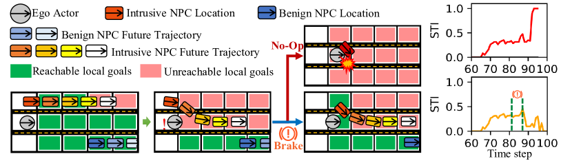
Figure 1: Safety threat indicator (STI) for a cut-in driving scenario with (a) safety mitigation controller (SMC) disabled (No-Op), and (b) SMC enabled (which decides to brake). Each reachable grid (local goal location) represents a safe navigational path (from current location to goal location) while the path to unreachable grids are unsafe paths. The goal of the SMC is to maximize the number of available safe navigational choice so as to create the safety blanket around the AV.

The contributions are:

1. Formalizing STI. To the best of our knowledge, this is the first attempt at using counterfactual reasoning to characterize the importance of each actor with respect to safety of the AV. The results are then used to proactively mitigate the safety hazards by taking precautionary actions.

2. NN-based STI evaluation for meeting realtime latency requirements. Estimating STI to meet latency deadlines is computationally intractable because STI requires reachability analysis which is P-SPACE hard lavalle1998rapidly . To solve this problem, we develop a neural network (NN) based approximation technique for estimating STI that is up to 414× faster than traditional, planner-based 5509799 STI estimation while achieving over $90\%$ accuracy on trained data. Given the low latency, STI can be used for monitoring and actively critiquing an AV’s decisions.

3. Demonstration of STI on real world driving datasets. We evaluate the proposed indicator on Argoverse dataset Chang_2019_CVPR to extract safety-threatening actors and driving scenarios. For example, we find that only 0.257% of the actors and 4.75% of the driving scenarios have STI of $\geq 0.9$.

4. Demonstration of SMC in simulation. We demonstrate SMC (along with STI estimation) on Carla simulator and show that SMC enables an AV to reduce the number of accidents from 565 to 128 out of 1000 driving scenarios, a $77.3\%$ reduction in the accident rate.

1.1 Related work

Actor importance. There is an increased focus on developing metrics to identify important actors.  Philion_2020_CVPR ; piazzoni2020modeling focus on evaluating the impact of the perception subsystem’s accuracy and uncertainty on the downstream tasks of driving. In particular, Philion et al. Philion_2020_CVPR design a planning-centric metric based on ablation methods to understand how uncertainty in actor states can lead to significantly different planning outcomes. Such a metric can be used to understand the importance of each actor, but it is not entirely satisfactory because (i) it is limited to improving the perception subsystem rather than safety of the overall system and (ii) it is agent dependent. In contrast, STI has different goals: (i) adaptability, i.e., STI is independent of the agent’s architecture, (ii) safety-oriented, i.e., STI explicitly encodes the impact of an actor or a scene on AV’s safe execution.

Proactive maintaining of safety. There are mainly two categories of work here: (i) identifying the safe distance from other actors, assuming everyone follows the “duty-of-care” policies, and (ii) identifying out-of-training-distribution (OOD) scenarios so as to plan for the worst case in order to avoid collisions. Duty-of-care approaches, such as Safety Force Field (SFF) SafetyForceField and Responsibility-Sensitive Safety (RSS) shalev2017formal , are geared towards estimating the safe distance from other actors assuming that everyone follows rules of the road. Additionally, the goal is to identify the culprit in case of a safety hazard. OOD models, such as pmlr-v119-filos20a , are geared toward identifying driving scenarios in which the ego actor’s future trajectory (i.e., plan) has significant variance. Such variance can be characterized using an ensemble of models or diverse data. Under high variance, the ego actor chooses to use the most pessimistic plan in order to avoid collisions.

None of the above approaches proactively try to ensure that multiple safe navigational choices are available to the AV. In contrast, our goal is to proactively create a safety blanket around the AV, by ensuring that the AV has multiple navigational choices. Our approach is not dependent on the underlying agent used by the AV. This allows the AV’s agent to focus on complicated navigating by obeying the rules of the road tasks while the SMC focuses on safety.

2 STI Formulation

Here we propose and formalize the safety threat indicator (STI) that quantifies the threat posed by an actor (and the driving scene) using causal and counterfactual reasoning. This indicator allows us to rank the actors and driving scene in terms of the danger they pose to the AV, thus allowing us to develop attention-based safety and mitigation techniques. We characterize the STI of an actor in terms of the decrease in driving flexibility caused by that actor. Driving flexibility is defined as the number of unique driving trajectories (or actions) available to the ego actor up to time horizon $k$ in the future at each time step. Thus, the greater the decrease in driving flexibility caused by an actor, the higher that actor’s STI.

Determining STI in the oracle setting.

We will first formalize the STI for an oracle setting in which the past, current, and future states of the actors are known with certainty. The oracle setting is suitable for offline assessment on prerecorded datasets where the ground truth labels are available. Let us assume that (i) there are $N$ actors in the world including the ego actor, (ii) we denote the state of an actor $i$ at time $t$ by $x^{(i)}_{t}\in\mathbb{R}^{3}$, and (iii) we denote the trajectory (i.e., trace of an actor’s state over time) from time $t$ to $t+k$ as $X^{(i)}_{t:t+k}$. Let us further denote the set of trajectories of all actors except the ego actor from time $t$ to $t+k$ by $\mathbb{X}_{t:t+k}=\{X^{(1)}_{t:t+k},...,X^{(N-1)}_{t:t+k}\}$. Let us further assume that (iv) we have access to ground truth information of $\mathbb{X}_{t:t+k}$ and an oracle local planner $f_{planner}$ that uses the trajectories of all the other actors from time $t$ to $t+k$, $\mathbb{X}_{t:t+k}$, and the position of the ego actor at time $t$, $x^{ego}_{t}$, to generate a set of future trajectories $\mathbb{Z}_{t:t+k}$ that the ego actor can follow safely from time $t$ to $t+k$ while obeying all the rules of the road (eq. 1). Since the oracle planner $f_{planner}$ is a theoretical model, a practical implementation of eq. 1 is discussed later in section 2.1.

$$Z_{t:t+k}=f_{planner}(\mathbb{M},\mathbb{X}_{t:t+k},x^{ego}_{t})$$ (1)

We can now construct a counterfactual query using eq. 1 in which we want to estimate the effect of removing $i^{th}$ actor (to understand the importance of the $i^{th}$ on safety) or all actors (to understand the importance of the driving scene) on $\mathbb{Z}_{t:t+k}$. The set consisting of all the navigable future trajectories in the absence of all actors, denoted $Z^{\varnothing}_{t:t+k}$, can be obtained using eq. 1 with $\mathbb{X}_{t:t+k}=\varnothing$. Similarly, the set consisting of all navigable future trajectories in the absence of the $i^{th}$ actor, denoted $\mathbb{X}^{/i}_{t:t+k}$, can be obtained using eq. 1 with $\mathbb{X}_{t:t+k}=\mathbb{X}^{/i}_{t:t+k}$, where $\mathbb{X}^{/i}_{t:t+k}$ is the actor trajectory set that contains trajectory of all actors except the $i^{th}$ actor.

We can now define the STI of a specific actor $i$ from time $t$ to $t+k$ as:

$$\rho^{(i)}_{t:t+k}=\frac{|Z^{/i}_{t:t+k}|-|Z_{t:t+k}|}{|Z^{\varnothing}_{t:t+k}|}$$ (2)

where $|\cdot|$ denotes the cardinality of the set. $|Z^{\varnothing}_{t:t+k}|$ is the normalization constant that forces the range to $[0,1]$ and enables us to compare STI across different driving scenarios. The STI value of $0$ means actor $i$ does not constraint the Ego actor’s driving flexibility. STI value of $1$ means that actor $i$ constraints the Ego actor’s driving flexibility such that there is no viable driving trajectory.

We can similarly define the total STI, $\rho_{t:t+k}$, of a driving scene per time step $t$ as the normalized reduction in future trajectories due to presence of all actors on the road.

$$\rho_{t:t+k}=\frac{|Z^{\varnothing}_{t:t+k}|-|Z_{t:t+k}|}{|Z^{\varnothing}_{t:t+k}|}$$ (3)

Determining STI in the realtime setting.

We now extend the formalism for realtime setting in which the precise locations of the actors are not known and in which one can only approximate the past, the current, and the future states of the actors using sensor measurements and predictive models, which include uncertainties. In a realtime setting, instead of point estimates (as discussed in section 2), we deal with probability distributions that allow us to model the noise. The complete derivation is provided in Supplementary Material.

2.1 Implementation of STI for realtime setting

Designing $f_{planner}$ is computationally intractable because the oracle planner is expected to output the set of all future safe trajectories (countable infinite), which is P-SPACE hard. Therefore, we propose following two heuristics: (i) a relaxed formulation that allows us to compute STI using planners employed in practice such as RRT lavalle1998rapidly , FOT 5509799 , and Hybrid A* dolgov2008practical and (ii) a data-driven model that enables realtime STI evaluation.

STI evaluation using practical planners.

Instead of calculating all viable future trajectories to the goal location, we propose to calculate reachable alternative locations (hereafter, referred to as the local goals) near the ego vehicle as a proxy representation of driving flexibility. These (local) goals are safe and represent intermediate locations that the ego vehicle can navigate to while trying accomplish its overall task of reaching the destination goal (global goal) safely. The local goals are the individual cells within the threshold distance $d$ of the current ego actor’s location in the bird’s-eye-view (BEV) of the drivable area that are potentially reachable given the time budget. Since $d$ has an upper bound given that the vehicle states, dynamic specifications, and number of grids in the drivable areas are fixed, the set of goals is also finite. This representation is a reasonable approximation of driving flexibility because the number of reachable local goals is positively correlated with the number of safe trajectories, and vice-versa. We denote the set of local goals that are potentially reachable with in the next $k$ time steps ($k$ is the time budget) as ${G}_{k}$. We can rewrite eq. 1 as a reachability evaluation of the set of local goals ${G}_{k}$ given a reachability solver $f_{reach}$. The reachability solver $f_{reach}$ classifies each goal $g_{k}\in{G}_{k}$ as either reachable or not-reachable and returns the set of reachable local goals ${R}_{k}=\{g_{k}|g_{k}\in{G}_{k},g_{k}\text{ is reachable between }t\text{ and }t+k\}$ given the time budget $k$ (eq. 17).

$${R}_{k}=f_{reach}(\mathbb{M},\mathbb{X}_{t:t+k},x^{ego}_{t},{G}_{k};\hat{f}_{planner}),{R}_{k}\subseteq{G}_{k}$$ (4)

We can then rewrite eq. 2 by replacing the set of safe trajectories $Z_{t:t+k}$ with the set of reachable local goals ${R}_{k}$ for STI evaluation as

$$\rho^{(i)}_{t:t+k}=\frac{|R^{/i}_{k}|-|R_{k}|}{|R^{\varnothing}_{k}|}$$ (5)

Similarly, we can rewrite eq. 3 as

$$\rho_{t:t+k}=\frac{|R^{\varnothing}_{k}|-|R_{k}|}{|R^{\varnothing}_{k}|}$$ (6)

with $R^{\varnothing}$ and $R^{/i}_{k}$ being the set of reachable local goals in the absence of all other actors and a particular actor $i$, following the same reasoning of $Z^{\varnothing}_{t:t+k}$ and $Z^{/i}_{t:t+k}$, respectively. The reachability problem in eq. 17 can be solved efficiently using a practical planner $\hat{f}_{planner}$ lavalle1998rapidly ; 5509799 ; dolgov2008practical (treated as parameters of $f_{reach}$) given the current ego actor state $x^{ego}_{t}$, the states of the actors $\mathbb{X}_{t:t+k}$, the drivable areas $\mathbb{M}$, and the ego actor’s dynamics capabilities (as part of the planner parameters). Depending on the problem setting, $\mathbb{X}_{t:t+k}$ can either be the ground truth actor states from a labeled dataset or the predicted states from the actors’ state histories (recall section 2).

STI approximation using a data-driven model.

The evaluation of STI using section 2.1 requires reachability analysis per actor per goal. Using a planner-based $f_{reach}$ to calculate the reachability of multiple local goals for multiple passes (each pass masks an actor) is not favorable because of (i) the computational complexity of the planner algorithm (P-SPACE hard despite the previous optimization) and (ii) the linear time complexity w.r.t. the number of local goals to be evaluate times the number of other actors in the scene. Since our ultimate goal is reachability evaluation, but not trajectory generation, to reduce STI evaluation latency we construct a neural network (NN) based reachability approximator (hereafter referred as the NN approximator), denoted $\mathcal{N}_{reach}$, to approximate the reachability calculation of the $f_{planner}$ (the FOT planner in our implementation). We choose to approximate reachability instead of the STI directly to preserve the interpretability of our formulation, i.e., help users of the model understand which local goals are reachable vs unreachable.

The input to $\mathcal{N}_{reach}$ consists of (i) a set of ego-actor-centered, bird’s-eye-view (BEV) images $\mathbf{I}_{t:t+k}$, that capture all the essential spatial-temporal information from time $t$ to $t+k$ of the scene and (ii) the ego actor’s state vector $\mathbf{e}_{t}$. $\mathbf{I}_{t:t+k}=\{I_{t},I_{t+1},...,I_{t+k}\}$ is constructed by stacking the BEV images from time step $t$ to time step $t+k$. The BEV image of a time step $t$, denoted ${I}_{t}$, captures drivable areas and the actors’ locations as spatial information. Stacking BEV images from multiple time steps allows the input data to capture the evolution of the actor’s future trajectories over time as temporal information. In addition, the current state of the ego actor, $\mathbf{e}_{t}=(v_{long},a_{long},v_{lat},a_{lat})$, encodes the velocity and acceleration information for the current time step as velocity impacts how far the vehicle can travel in the next $k$ time steps. Since the reachability analysis uses an ego-centered coordinate frame, the location of the ego actor is not needed. Given $\mathbf{I}_{t:t+k}$ and $\mathbf{e}_{t}$ the model $\mathcal{N}_{reach}$ outputs the reachability indicator vector $\mathbf{r}_{k}$ for the current time step:

$$\mathbf{r}_{k}=\mathcal{N}_{reach}(\mathbf{I}_{t:t+k},\mathbf{e}_{t})$$ (7)

Each element of the reachability indicator vector $\mathbf{r}_{k}$ is a binary value indicating whether a local goal location in the input BEV image $I_{t}$ is reachable. Hence we formulate the reachability problem as a binary classification problem per $\mathbf{r}_{k}$ element, where the goal of the NN is to classify each cell in the grid (or each element of $\mathbf{r}_{k}$) as reachable verses not-reachable. Therefore, given a ground truth indicator vector label $\mathbf{r}^{*}_{k}$, the objective function to minimize is

$$l(\theta)=\sum_{b\in\mathcal{B}}BCE(\mathbf{r}^{(b)}_{k},\mathbf{r}^{*(b)}_{k})=\sum_{b\in\mathcal{B}}BCE(\mathcal{N}_{reach}(\mathbf{I}^{(b)}_{t:t+k},\mathbf{e}^{(b)}_{t};\theta),\mathbf{r}^{*(b)}_{k})$$ (8)

where $BCE(\cdot)$ stands for binary cross-entropy loss and $\mathcal{B}$ is the mini-batch. The ground truth labels $\mathbf{r}^{*}_{k}$ can be generated using the $f_{reach}$ with $\hat{f}_{planner}$ following section 2.1. Note that to ensure a fixed size $\mathbf{r}_{k}$, instead of discretizing the drivable area as in section 2.1, we discretize the entire BEV image space. We do this because the BEV image size is fixed, while the drivable area size can vary. The detailed generation of $\mathbf{I}_{t:t+k}$ as well as $\mathbf{r}_{k}$ is provided in the Supplementary Material. Finally, given the predicted reachability indicator vector $\mathbf{r}_{k}$, we can assess whether a goal location in the BEV image space is reachable and hence calculate the actors and the scene STI using eqs. 5 and 6.

3 RL-based Mitigation for Safety-Critical Scenarios

Safety-critical scenarios are scenarios that can result in serious safety violations teslaCrash ; uberCrash ; banerjee2018hands if not handled properly. Here we describe the model and architecture of our proactive safety-hazard mitigation controller (SMC). SMC uses RL and STI to perform mitigation actions in safety-critical scenarios. The SMC is a standalone module that executes alongside the ego actor and intervenes with mitigation actions when necessary. The overall architecture of SMC is shown in fig. 2.

To illustrate the execution model with the SMC, suppose we have a ego actor denoted as $\mathcal{A}$ that is capable of handling normal driving scenarios. At each time step $t$, $\mathcal{A}$ consumes the state $\mathbf{S}_{t}$ and perform a driving action $da_{t}$: $da_{t}=\mathcal{A}(\mathbf{S}_{t})$. The SMC, denoted $\mathcal{M}$, also consumes some state $\mathbf{S^{\prime}}_{t}$ (which can be the same as $\mathbf{S}_{t}$) and provides a mitigation action $ma_{t}$ based on its policy: $ma_{t}=\mathcal{M}(\mathbf{S^{\prime}}_{t})$. $ma_{t}$ overwrites $da_{t}$ if $ma_{t}$ is not the "no-operation" (No-Op) action. So for the final action $a_{t}$ on $\mathbf{S}_{t}$:

$$a_{t}=da_{t}\text{ if }ma_{t}==\text{No-Op}\text{ else }a_{t}=ma_{t}$$ (9)

Next we define the state, action space, state transitions, and reward function used to learn the policy.

State space: The state $\mathbf{S}_{t}\in\mathbb{S}$ at time $t$ captures the spatial-temporal information of the SMC’s environment, including other actors and drivable areas. It could be the internal world of the ego actor or a direct sensor measurement such as camera images (section 4.2.2) or LiDAR cloud points. The design can be flexible depending on what information is available.

Action space: The action space $\mathbb{A}$ of the SMC consists of mitigation actions; this includes but is not limited to emergency-braking ($EB$), lane-change-to-left ($LCL$), lane-change-to-right ($LCR$), accelerate ($ACC$), etc., plus no-operation (No-Op). Note that No-Op is needed because it provides the SMC with the option of not performing mitigation in non-safety-critical situations. In this work the actions are discrete, in which case the actions’ trajectories and low-level controls are predefined and the SMC selects which action to perform.

State transition function: The state transition function $f_{transit}:\mathbb{S}\times\mathbb{A}\rightarrow\mathbb{S}$ calculates the next state $\mathbf{S}_{t+1}$ given the current state $\mathbf{S}_{t}$ and action $ma_{t}$ pair: $\mathbf{S}_{t+1}$ = $f_{transit}(\mathbf{S}_{t},ma_{t})$. Here, $f_{transit}$ is provided by the driving simulator carla17 ; lgsvl . At each time step, the simulator provides $\mathbf{S}_{t}$ for the actor to act. The actor acts on $\mathbf{S}_{t}$ based on its policy, and the simulator upon receiving the action updates the scenario and provides $\mathbf{S}_{t+1}$.

Rewards: At each time $t$, a reward $r_{t}$ is generated based on the state-action pair. To effectively learn a mitigation policy that minimizes the scenario STI over time, we use STI as part of the reward function. In addition, the reward function is constructed to encourage normal driving and to penalize mitigation actions in low STI situations. A generic reward is as follows:

$$r_{t}=\alpha_{0}(1-STI)+\alpha_{1}r_{pc}+\alpha_{2}p_{am}+\alpha_{3}r_{comfort}+...+\alpha_{n}r_{nth\_factor}$$ (10)

where $\alpha_{0}...\alpha_{n},\alpha_{i}\geq 0,\sum_{i=0}^{n}\alpha_{i}=1$ are constant weights of each term that controls trade-offs. $STI,r_{pc},p_{am}$, and $r_{comfort}$ are STI values of the scene, reward for path-completion, penalty for activation of mitigation, and reward for maintaining comfort, respectively. Note that the third term penalizes frequent activation of mitigation actions because safety-critical situations are rare and mitigation should only be activated when it is truly needed, to avoid affecting normal driving. The general formulation also shows additional performance indicator terms that can be customized for different use-cases. The definitions of $r_{pc}$, $p_{am}$, and $r_{comfort}$ used in our implementation are found in Supplementary Material.

4 Experiment Setup

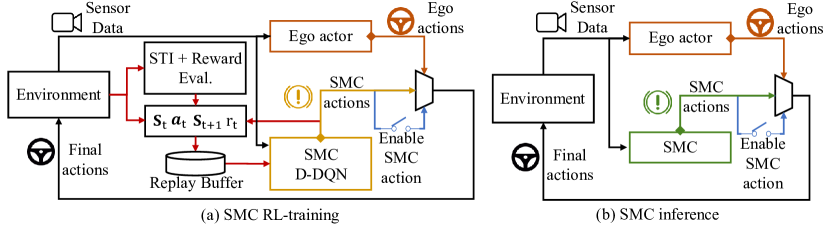
Figure 2: Overview of the SMC framework: (a) RL-based SMC training with Double DQN and experience replay, (b) Runtime SMC inference

This section describes in detail the dataset, training, and evaluation (also shown in fig. 2 ).

4.1 Dataset and driving scenarios

Real-world dataset.

We characterize the Argoverse real-world dataset Chang_2019_CVPR to evaluate the bias that exists in such datasets towards safer scenarios. Such bias exists because the vehicles used in these datasets are controlled (or monitored) by humans who tend to avoid dangerous scenarios. The Argoverse dataset consists of $50+$ driving scenes, $300$K actor annotations, and HD-map information. The Argoverse dataset is also used to train and evaluate the NN-based reachability approximator.

Simulator-generated dataset.

The real-world datasets consist of prerecorded data that (i) do not provide a complete control-feedback loop and (ii) lack safety-critical scenarios with high actor or scene STI values (refer to section 5.1). Therefore, we use Carla carla17 to simulate and collect data on safety-critical scenarios. We simulate the cut-in scenario from the NHTSA precrash scenario typology report najm2007pre as the base scenario because it ranks among the top scenarios for financial loss and fatality rate. In the cut-in scenario, one of the NPC actors is approaching from behind the ego actor but in the adjacent lane, and then the NPC actor cuts in front of ego actor closely as it passes the ego actor. Such a cut-in scenario is highly hazardous due to the limited reaction time available before collision. Note that there are multiple other NPC actors but those are not as hazardous as the ones that are cutting in. The base scenario defines the overall scenario typology, but the level of safety criticality may vary depending on the scenario’s hyper-parameters such as (i) cut-in distance, (ii) cut-in speed, (iii) cut-in angle and (iv) the distance between the ego actor and the NPC actor at the start of the scenario. Therefore, to stress test our proposed methodology, we generate 1000 mutated scenarios based on the base scenario by varying the above hyperparameters (described in Supplementary Material). These mutated scenarios are used to (i) evaluate the correlation between the STI (refer to section 2) and the safety criticality of the scenarios, (ii) train and evaluate the NN-based reachability approximator, and (iii) train and evaluate the RL-based SMC. For each mutated scenario, we run the same ego actor (the LBC agent chen2019lbc ). Hereafter, we will refer to the resulting dataset as the mutated scenarios dataset.

4.2 Training procedure

4.2.1 NN-based reachability approximator

Inputs and outputs: We train and evaluate the approximator on both the real-world dataset and the simulated mutated scenarios dataset. We use the bird’s-eye-view (BEV) to represent the drivable area along with the NPC actors as the input $\mathbf{I}_{t:t+k}$ to the approximator. Note that we need the ground truth labels, in this case the reachability indication vector $\mathbf{r}_{k}$, to train the approximator using the loss function eq. 8. We generate these ground truth labels using FOT planner 5509799 to calculate the reachability for each input $\mathbf{I}_{t:t+k}$. We choose the FOT planner because it considers physically realistic trajectories given the ego actor’s dynamics and the time horizon $k$ for the reachability calculation.

Model architecture: The approximator uses the ResNet-34 resnet34 as the feature extractor to extract information from the input $\mathbf{I}_{t:t+k}$ (see eq. 7). We replace the fully connect layers for classification with a customized output head to convert the extracted feature into the reachability indication vector $\mathbf{r}_{k}$ (see eq. 7). Please see the architectural details in the Supplementary Material.

Training procedure: We do $80\%-20\%$ training-validation split to assess the approximator’s accuracy. We train the model for 750 epochs with per $\mathbf{r}_{k}$ element Binary Cross-entropy loss as the criterion and the Adam Optimizer kingma2014adam with a learning rate of $1e^{-5}$ to optimize the model parameters.

4.2.2 RL-based SMC

Inputs and Outputs: The RL-based safety harzards mitigation controller (SMC) is implemented based on the design in section 3. The state representation $\mathbf{S}_{t}$ of the environment is the same as the input (three front-facing camera images) to the ego actor (LBC agent) except that we convert the images to grayscale as the input instead of using the RGB format. To embed temporal information as part of the state representations, we follow the method outlined in mnih2013playing , in which the authors concatenate the grayscale camera data plus the planner target heatmaps from 4 previous time steps. At each time step $t$, the SMC $\mathcal{M}$ consumes the state and outputs a mitigation action $ma_{t}$ based on its mitigation policy.

Model architecture: The SMC follows  mnih2013playing , in which a CNN ($V$) with parameter $\phi$, denoted $V_{\phi}$, is used as the function estimator to approximate the $Q(S,a)$ values for all actions given $\mathbf{S_{t}}$:

$$Q(a_{t},\mathbf{S_{t}};\phi)=V_{\phi}(\mathbf{S_{t}})$$

In our implementation, $V_{\phi}$ uses a similar backbone as the ego actor with less input channel due to the usage of grayscale input images. We modify the output head to output the same size as the action space $\mathbb{A}$ to predict the $Q$ values for all possible actions in one shot. At inference time, the action with the maximum $Q$ value is chosen. More details are available in Supplementary Material.

Training procedure: We train the SMC on the simulated cut-in scenario by executing 100 episodes of a mutation with hyperparameters equal to the median value of the individual hyperparameters across the previously generated 1000 mutations of the cut-in scenario (which is described in  section 4.1). At each training time step, the mitigation actor (SMC) observes the state and select mitigation activation based on the learned policy. If mitigation is activated ($ma_{t}\neq\text{No-Op}$), the control output by the ego actor is overridden by the SMC’s mitigation action (eq. 9). Note that we do not modify the policy of the ego actor but only train the SMC. Since the reward function depends on the STI values evaluation per frame, in order to run the training closer to realtime, we use the CNN-approximator to evaluate the scene STI values per time step given its high accuracy (see section 5.2). Finally, the Double-DQN DBLP:journals/corr/HasseltGS15 training algorithm with replay buffer is used for faster convergence.

5 Results

5.1 Characterization of STI values

We characterize the STI of the actors and the scenes for both the real-world and the variant scenarios datasets in section 4.1. The FOT planner-based STI evaluator is used to characterize the STI value of all datasets in an offline setting to maximize accuracy.

5.1.1 Real-world dataset

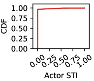
(a)  

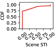
(b)  

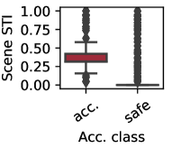
(c)  

Figure 3: (a)(b) STI CDF of Argoverse dataset: (a) Actor STI (b) Scene STI; (c) STI distribution vs accident class of the cut-in scenario; acc.: mutations with accidents, safe: mutations w/o accidents.

We evaluate the STI values of (i) each actor in a driving scene (per time step) and (ii) each driving scene (per time step) across all driving scenes in the Argoverse dataset. According to the evaluation results, the $50^{th}$, $75^{th}$, $90^{th}$, and $99^{th}$ percentiles of the actor STI values are 0.0, 0.0, 0.0, and 0.4, respectively, while the $50^{th}$, $75^{th}$, $90^{th}$, and $99^{th}$ percentiles of the scene STI values are 0.0, 0.071, 0.454, and 0.99 respectively, as depicted in the CDFs of the STI value distribution in figs. 3(a) and 3(b).This means that at least $90\%$ of the actors or $50\%$ of the scenes have 0 STI values and that a high STI is rare and belongs to the long tail of the real-world datasets’ data distribution. This characterization exposes the current limitations of the state-of-the-art, real-world datasets when it comes to including a sufficient number of high STI actors and scenes for unbiased AV development as the datasets are biased towards safer scenarios; thus, it highlights the need for inclusion of such data and the need for a simulated dataset in cases where high STI actors and scenes can be generated in large numbers. Note that a scene’s overall STI can be high even when the importance of the individual actors is low, as multiple actors together can significantly reduce the driving flexibility of the ego actor. We will explain such examples in the Supplementary Material.

5.1.2 Simulated safety-critical dataset

We evaluate the STI values on the variant scenario dataset to understand the relationship between STI values and safety violations (accidents). fig. 3(c) shows the boxplot distribution of STI across all driving scenes per time step (calculated with eq. 6) for runs with and without accident. The figure shows that STI values are significantly higher in the scenes that lead to accidents in the future compared to those without, suggesting that high STI and the chance of accident are positively correlated. Moreover, our analysis shows that the underlying distribution of STI is different between scenes that lead to accidents verses scenes that do not. This is verified by the statistical comparison using KS Two-sample Test on the distributions of STI from scenes that lead to accidents verses the STI from scenes that are safe, with a significance level of $0.05$. We can reject the Null-hypothesis of the KS Two-sample Test, as the resulted $p\text{-}value$ is <<$0.01$ (outputs 0.00 due to numerical underflow).

fig. 4(a) shows the probability that an accident will happen within the next $k$ time steps given a particular STI value for the cut-in scenario mutations. We can see a positive relationship between the STI values and the accident probability in the next $k$ time steps, which suggests that STI values are good indicators of imminent safety violations.

5.2 Evaluation of the NN-based reachability approximator

This section shows the evaluation results of the NN-based reachability approximator on both the real-world dataset and the variant scenarios dataset.

Dataset	Precision	Recall	F1-score
Argoverse	$0.83$	$0.87$	$0.85$
Mutated scenarios	$0.96$	$0.97$	$0.96$

(a) NN-based reachability approximator performance on testing datasets (described in section 4.1).

Mitigation policy	# acc./# T.runs
LBC	565/1000 (0.565)
LBC+SMC (ours)	128/1000 (0.128)

(b) Comparison of mitigation policies (i) LBC agent and (ii) LBC agent with SMC (ours); # acc.: #runs with accident, #T.runs: total runs.

Table 1: Table of results: (a) NN-based reachability approximator evaluation, (b) SMC evaluation.

table 1(a) summarizes the reachability approximation performance on both the real-world and the simulated datasets. The approximator performs worse for the real-world dataset because the HD-map information is not accurate compared to the simulator maps.

The NN-based approximator reduces the reachability compute latency on the real-world dataset by $99.8\%$ from $2.37\pm 0.0279$ seconds when using the $FOT$ planner-based evaluator to $0.00572\pm$3.50\text{\times}{10}^{-5}$$ seconds, a $414.34\times$ latency improvement, per time step per actor per goal. On the simulated dataset, the NN-based approximator reduces the reachability compute latency from $2.087\pm 0.0030$ seconds when using the $FOT$ planner-based evaluator to $0.00569\pm$2.15\text{\times}{10}^{-5}$$ seconds, a $366.7\times$ latency improvement.

5.3 Efficacy of RL-based safety mitigation controller

The strong correlation between the STI value and the probability of an accident suggests that STI value is a good indicator of an imminent accident. However, instead of mitigating only when the STI is high (reactive mitigation), it is more effective to proactively reduce the STI as outlined in section 3 to avoid high STI situations. table 1(b) shows the accident rate comparison between the ego actor (the LBC agent) with SMC, and the ego actor without SMC for the variant scenarios. The SMC reduces the accident rate from $0.565$ to $0.128$, a $77.3\%$ reduction, on the cut-in scenario mutations. This is reflected in the higher mean STI values of the variant scenario runs in which the ego actor without SMC leads to accidents, shown in fig. 4(b). Across the 1000 cut-in scenario mutation executions, the SMC reduces the scenario STI, which leads to a lower accident rate. Refer to Supplementary Material for illustrative examples of SMC-based mitigation.

The high mitigation efficacy in all variant scenarios suggests that the SMC can generalize to variant scenarios with similar topology but different hyperparameters. It achieves this efficacy by learning from just a few instances of the variant scenarios of that typology. In our case, the SMC is trained on one of the variant scenarios and evaluated on all variant scenarios (recall section 4.2).

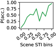
(a)  

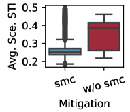
(b)  

Figure 4: (a) Accident probability $P(acc.)$ vs STI binned values of the cut-in scenario mutations, (b) Mean scene STI distribution with and without SMC of the cut-in scenario mutations

6 Conclusion and Future Work

We proposed a novel safety-threat indicator (STI) that allows us to identify risky actors and driving scenarios. Using STI as a basis, we developed a safety-hazard mitigation controller (SMC) to maximize safety for an AV by focusing on the actors most threatening to the AV’s safety. The SMC’s execution is independent of the existing AV controller, so it does not interfere with normal AV operations. Our future work will address limitations and explore further use-cases of STI for other autonomous driving tasks.

Three areas remain to be addressed. First, the proposed indicator (and hence the controller) assumes that each navigational choice is equally safe. However in practice, certain choices are safer than others. For example, in our grid formulation, we can estimate time-to-collision in each grid to further rank each path (i.e., each trajectory from the current position to one of the grid locations). Second, the SMC was only trained and evaluated in simulation. Given the hazardous nature of these scenarios, there is a need to evaluate the robustness of the proposed controller in a real-world, on-road environment and identify techniques to transfer the model from simulation to the real world. And third, we need to evaluate the sensitivity of STI to different planners for evaluating reachability (e.g., R2P2 Rhinehart_2018_ECCV and RRT lavalle1998rapidly ). In the future, we will both address these limitations and apply STI in other use-cases, including the following: STI can assist with rare test dataset/benchmark generation for autonomous driving tasks. For example, STI can be integrated with fuzzing and adversarial techniques to identify cases in which AVs will collide 9564360 ; 9251068 . STI can also be directly integrated into the planner fisac2019hierarchical , alleviating the need for the mitigation controller. And finally, STI can be integrated with systems like PyLot pylot and others li2020towards for deadline-aware scheduling tasks.

Appendix

Mitigation policy	# acc./# T.runs
LBC	565/1000 (0.565)
RIP (WCM)	478/1000 (0.478)
LBC+SMC (ours)	128/1000 (0.128)

Table 2: Comparison of mitigation policies (i) LBC agent chen2019lbc , (ii) RIP agent with the worst case model (WCM) pmlr-v119-filos20a , and (iii) LBC agent with SMC (ours); # acc.: number of of runs with accident, #T.runs: total number of runs.

Appendix A Additional Experiments and Results

A.1 RIP agent as an additional baseline for SMC evaluation

In the main paper we compare the SMC’s mitigation efficacy with the baseline agent– the LBC agent by Chen et. al. chen2019lbc . Here we add the RIP agent by Filos et. al. pmlr-v119-filos20a as an additional baseline ego actor for comparison. Since authors only provides the training dataset and training code but not the model weights, we train the RIP agent on the provided training dataset using 4 ensemble models. Note that the authors do not provide the number of epochs used for training each model, so we train each model until the loss converges. We compare our SMC with the RIP-worst case model or RIP-WCM as it is the best performing model in pmlr-v119-filos20a .

Similar to the LBC agent, we evaluate the RIP agent on the $1000$ mutated scenarios with the same simulation environment and hardware and report its accident rate in table 2. Though out performing the LBC agent, the RIP agent results in a high accident rate of 0.478 comparing to the LBC+SMC (our) approach which results in an accident rate of 0.128 on the same mutated scenarios. Our approach reduces the accident rate by 73.2% compared to the RIP agent.

The RIP agent improves safety by leveraging the fact that out of distribution data (OOD) leads to higher epistemic uncertainty, and hence the agent should act conservatively. In the WCM ensemble setting, the RIP agent acts according to the most permissive plan and this can lead to recovery from out of data distribution. There is a possibility that the detection of the distribution shift is not done sufficiently in advance and, therefore, there might not be any safe trajectory available to the ego agent at the time of detection. In other words, even the most permissive plan is not safe; thereby, leading to accident as evident from our evaluation. Instead, the SMC learns the mitigation actions by embedding the knowledge of STI–an indication of safety threatening situation–as part of its policy which enable it to mitigate dangerous situations (recover from OOD) more effectively. Moreover, we assert that the SMC approach is orthogonal to approaches like RIP or LBC and they can be applied simultaneously to improve safety and robustness of autonomous driving.

A.2 SMC mitigation action illustration with an example

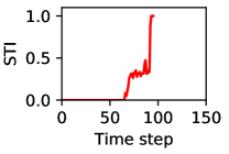
(a)  

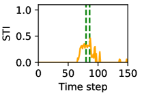
(b)  

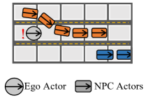
(c)  

Figure 5: Scene STI time series of a mutated scenario run. (a) shows scene STI in red without SMC enabled. (b) shows scene STI with SMC enabled and mitigation period between dashed lines. (c) Shows the moment of cut in typology.

Here we show an example activation of the SMC’s mitigation action. SMC proactively applies emergency braking proactively to reduce the STI in a safety critical scenario and, hence, avoids the accident which otherwise would happen (using the LBC as the ego actor). fig. 5 plots the scene STI of the scenario per time step. In fig. 5(b), the orange line represents the running scene STI with the SMC enabled and the green dashed vertical lines shows the start and the end of the mitigation action period. The red line in fig. 5(a) represents the running STI without SMC for comparison.

In this run, as the threatening NPC actor approaching from behind the ego actor at a higher speed, the driving flexibility decreases (STI increases) at the $60^{th}$ time step. At around the $80^{th}$ time step right before the cut in happens, the STI starts to increase (in both figs. 5(b) and 5(a)) and subsequently the SMC intervenes and brakes in fig. 5(b) (after the first green vertical line) to reduce the STI and avoid possible accident, and SMC then disengages as the situation alleviates (after the second green vertical line) and the ego actor continues to drive to its destination. Without the SMC, the ego actor alone fig. 5(a) (using only the LBC agent) fails to recognize this adverse situation and misses the mitigation window, resulting in an accident. We can see in fig. 5(a) the STI continues to increase (i.e., red line continues to climb) until the time of the accident ($100^{th}$ time step) after which the simulation terminates.

A.3 High STI scenes from real-world dataset

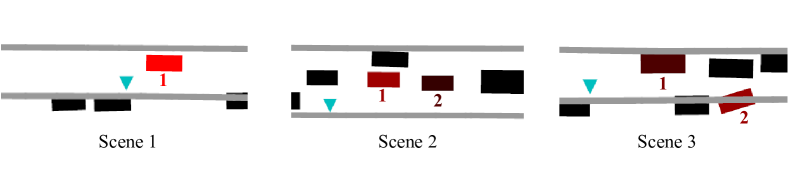
Figure 6: BEV representation of real-world high STI scenes from Arogverse dataset. Here, the blue triangle represents the ego actor and the rectangles represents NPC actors. The redness of an NPC actor indicates the STI value–the brighter the red color, the higher the STI of that NPC relative to other NPC actors’ STI in that scene. Labeled NPC actors with non-zero STI are labeled.

Recall from section 5.1.1 that we evaluate the actors’ and the scenes’ STI on the Argoverse real-world dataset. The result show that high STI actors or scenes are rare because real-world datasets are collected in a safe environment with human supervision. We extract those rare scenarios and actors using our proposed indicator.

We find that a scene STI can be high even with low STI actors in safety-critical configurations. Here we show examples of high STI scenes, as BEV representations, from the Argoverse dataset and provide the reasons why the scenes’ STI are high based on the actors configuration and the actors’ STI by exploiting the interpretability of our formulation.

Scene 1: High scene STI due to one actor.

In the first scene (fig. 6 Scene 1), the ego actor travels on the lane with NPC actor 1 traveling closely in the adjacent lane. The scene STI of this scene is $0.643$. The actor STI for NPC actor 1 is $0.642$, with other actors having 0 STI. In this case, the NPC actor 1’s STI is high because it travels closely with the ego actor which reduces the ego actor’s driving flexibility considerably. Moreover, the NPC actor 1 is solely responsible for the high scene STI because the ego actor’s driving flexibility is constraint mainly by NPC actor 1, while other NPC actors have limited affect on the ego actor’s driving flexibility.

Scene 2: High scene STI due to the presence of NPC actors in the close vicinity.

In the second scene (fig. 6 Scene 2), the ego actor travels on a multi-lane busy highway. NPC actor 1 and 2 are traveling in the same direction on the left adjacent lane in close vicinity. The scene STI of this scene is high at $0.625$. However, the actor STI for the NPC actor 1 and 2 are relatively low compared to the scene STI at $0.19$ and $0.063$ respectively, with other NPC actors having 0 STI. Note that the sum of individual actor STI does not need to be equal to the scene STI because the reduction in the ego actor’s driving flexibility is jointly constrained by the individual actor’s trajectories. In this case, the scene STI is high because the driving flexibility is greatly constraint by NPC actors 1 and 2 jointly and the ego actor can only stay in its own lane. Removing all NPC actors in the scene greatly improves driving flexibility as the ego actor can now chose to merge left. On the other hand, the STI of each individual NPC actor (NPC actor 1 and 2) is low because each NPC actor only contributes partially to the reduction of the ego actor’s driving flexibility so removing only one NPC actor only increase the driving flexibility marginally. For example, removing NPC actor 1 only frees up the adjacent space near to the ego actor, the ego actor is still constraint by NPC actor 2. Finally we can see that the actor’s STI distribution is sensitive to distance which a higher STI is assigned to the closer actor (NPC actor 1) as it limits the driving flexibility more than NPC actor 2 that is farther ahead.

Scene 3: High scene STI due to the intrusive driving maneuver of NPC actors.

In the third scene (fig. 6 Scene 3), the ego actor travels on the right lane going straight with some NPC actors stopped on the left lane waiting to turn left and some NPC actors park on the right. In particular, NPC actor 1 stops on the left lane waiting to turn left, and NPC actor 2 starts merging from the parking lane into the ego lane. The scene STI is high at $0.64$, while NPC actor 1 and NPC actor 2 have STI of $0.09$ and $0.18$, receptively. As Scene 2 described above, the scene STI is high because the ego actor’s driving flexibility is constraint by the NPC actors and in this case collectively and the ego actor can only choose to merge left and stop or continue on the same lane. On the other hand, the individual NPC actor’s STI are low because removing each of the NPC actor (NPC actor 1 or 2) only improves the driving flexibility marginally, with other NPC actors still constraining the ego actor’s driving flexibility. However, Different from Scene 2, the actor’s STI distribution in this scene is sensitive to motion as the NPC actor 2, the actor that starts driving and merging in front of the ego actor, is assigned a higher STI value than the NPC actor 1, which stops for traffic light, despite NPC actor 1 is closer to the ego actor.

Appendix B STI Formulation in the Realtime Setting

This section outlines the detailed derivation of STI evaluation in the realtime setting as a supplementary to section 2. Recall that in the oracle setting we assume that the set of trajectories of all actors from $t=0$ to $t=T$, $\mathbb{X}_{t:t+k}$, is precisely known (without uncertainty). This assumption does not hold in the realtime setting in which the actors’ past, current, and future states by nature are noisy as they are estimated from realtime sensor measurements. Hence, we extend our formulation of the oracle setting to account for the actors’ noisy state estimations and trajectory set, as follows.

Obtaining $\bar{X}^{(i)}_{t:t+k}$ for an actor.

Recall that $\bar{X}^{(i)}_{t:t+k}$ is the set of states from $t$ to $t+k$ of actor $i$. In the realtime setting, the ego actor uses the past and the current state measurements $o_{0:t}^{(i)}$ to estimate the current state $\bar{x}^{(i)}_{t}$ of an actor. Note that $\bar{x}^{(i)}_{t}$ is different from $x^{(i)}_{t}$ (defined in the oracle setting in section 2), as $\bar{x}^{(i)}_{t}$ captures the uncertainty/noise associated with the state. The horizontal bar on the top of the symbols is used here to distinguish between the noisy state data and ground truth state data. Typically, $o_{t}^{(i)}$ is the bounding box that is detected using object-detection algorithms, such as YOLO redmon2018yolov3 , and $\bar{x}^{(i)}_{t}$ is estimate using a state-space estimation algorithm $f_{esitmate}$, such as Kalman Filter welch1995introduction from measurement history $o_{0:t}^{(i)}$. The future states of an actor $i$ from time $t$ to time $t+k$ can then be predicted given a state prediction model $f_{predict}$ and the actor’s state estimation history $\bar{x}^{(i)}_{0:t}$:

$$\bar{X}^{(i)}_{t:t+k}=f_{predict}(\bar{x}^{(i)}_{0},...,\bar{x}^{(i)}_{t})=f_{predict}\left(f_{esitmate}(o^{(1)}_{0},...,o^{(N)}_{t})\right)$$ (11)

Alternatively, given that state estimations and predictions often follow the algorithm’s underlying noise assumptions welch1995introduction , $\bar{X}^{(i)}_{t:t+k}$ can also be modeled by the probability distribution shown in eq. 12

$$\bar{X}^{(i)}_{t:t+k}=P(\bar{x}^{(i)}_{t},...,\bar{x}^{(i)}_{t+k}|o^{(1)}_{0},...,o^{(N)}_{t})$$ (12)

Constructing $\mathbb{Q}_{t:t+k}$ for STI evaluation.

Recall from above that $\bar{X}^{(i)}_{t:t+k}$ is the future state estimation distributions due to the noisy state estimation of an actor $i$, from time $t$ to $t+k$. Let $\mathbb{Q}_{t:t+k}$ denote the set consisting of samples of future trajectories for all actors, we can construct $\mathbb{Q}_{t:t+k}$ by sampling from $\bar{X}^{(i)}_{t:t+k}$ for each actor $i$ for all $i$:

$$\mathbb{Q}_{t:t+k}=\{{Q^{(1)}_{t:t+k}\sim{\bar{X}}^{(1)}_{t:t+k},...,Q^{(N)}_{t:t+k}}\sim{\bar{X}}^{(N)}_{t:t+k}\}$$ (13)

Following the oracle setting, let us assume that an oracle planner $f_{planner}$ exists and can generate all possible future trajectories that the ego actor can follow safely given $\mathbb{Q}_{t:t+k}$, $\mathbb{M}$, and ${x}_{t}^{ego}$ (eq. 14).

$$\bar{Z}_{t:t+k}=f_{planner}(\mathbb{M},\mathbb{Q}_{t:t+k},{x}^{ego}_{t})$$ (14)

Then we can evaluate the actor STI ($\rho^{(i)}_{t:t+k}$) and scene STI ($\rho_{t:t+k}$) with equation eq. 2 and eq. 3, respectively with the sampled trajectory set $\mathbb{Q}_{t:t+k}$.

Note that, for different sampled instances of $\mathbb{Q}_{t:t+k}$ with eq. 13 $\bar{Z}_{t:t+k}$ will be different. Therefore, we can estimate the uncertainty in the STI of an actor and the scene by sampling multiple instances of $\mathbb{Q}_{t:t+k}$ and executing eq. 2 and eq. 3 multiple times.

Appendix C BEV Representation of Driving Scenes

In order to compute STI based on reachability using commonly employed planners $\hat{f}_{planner}$ such as RRT lavalle1998rapidly , FOT 5509799 , and Hybrid A* dolgov2008practical , we need to represent the driving scene in planner recognizable formats. Here we show the construction of the BEV representation for the planner to consume in details.

Representing $\mathbb{X}_{t:t+k}$ and $x_{t}^{ego}$.

Referring to eq. 17, one part of our representation of the driving scene per time step $t$ includes the NPC actors’ projected future trajectories $\mathbb{X}_{t:t+k}$, and the current ego actor state $x_{t}^{ego}$. Collecting information for $\mathbb{X}_{t:t+k}$ and $x_{t}^{ego}$ is straight forward as these are either provided by the dataset’s ground truth labels or the state of a simulator (as ground truth labels) in the oracle setting, or by estimating them from the sensor measurements in the real-time setting. The state of an actor consists of the center location and the size of its bounding box. The state of the ego vehicle consists of the location, rotation, and the velocity.

Representing $\mathbb{M}$ and $G_{k}$.

The other part of our representation includes representing the map information $\mathbb{M}$ and the goal information $G_{k}$, as shown in eq. 17, in a planner consumable format. We represent $\mathbb{M}$ by dividing the map space into "drivable" and "non-drivable" areas. Drivable ares are road surfaces that belongs to a drivable lane, which includes the current ego lane (the lane that the ego actor is traveling on) and adjacent lanes traveling in the same direction. Non-drivable areas are road surfaces that are either non-drivable (e.g., passer-by or parking lots), or belong to lanes traveling in the other direction. For example, given a two way street, the lanes traveling in the same direction as the ego lane are drivable areas, and everywhere else are non-drivable areas. To constraint the planner to consider drivable path only, we further construct $B$ as a set of static obstacles from the lane boundaries.

We further divide drivable areas into a set of grids, denoted $C_{k}$. Each grid is of size $l\times w$ with the center of the grid being a potential goal location $g_{k}$, where $l$ is the length of the grid in the longitudinal direction of the lane, and $w$ is the width of the grid in the lateral direction of the lane. The choice of $l$ and $w$ can be flexible, for example, in our case for the Argoverse dataset which the length width is not specific, we choose $l=5$ meters and $w=3.7$ meters, corresponding to the common length of a family car and the common width of a motorway lane. The simulator dataset provides the lane width information to set $w$. Note that given the current ego actor state $x_{t}^{ego}$, its dynamic constraints, and the time budget $k$, the farthest distance $d$ that the ego actor can reach is governed by

$$d=|\mathbf{v}_{t}^{ego}|+k*|\mathbf{a}_{max}^{ego}|$$ (15)

given the lane is not infinitely wide, the number of grids that the ego actor can potentially reach is also finite. Moreover, it is a reasonable assumption that the ego actor should not plan to travel backward, so the set of potential goals $G_{k}$ given the time budget $k$ can be expressed as

$$G_{k}=\{g_{k}|g_{k}\text{ is of forward direction of ego actor }\cap dist(g_{k},x_{t}^{ego})\leq d,g_{k}\in C_{k}\}$$ (16)

Representation in ego coordinates.

For convenience, we transform the actor trajectories $\mathbb{X}_{t:t+k}$, the ego actor state $x_{t}^{ego}$, the set of potential goals $G_{k}$, and the set of static lane boundaries $B$ to ego-centered coordinates. That is, we first transform the locations of all the aforementioned sets by subtracting the ego actor’s location, and then we rotate them in the opposite direction of the ego actor’s rotation about the origin, per time step $t$. We can then drop the location and rotation element from the ego state since they are always zeros in the ego-centered coordinate system.

Given that $(G_{k},\mathbb{X}_{t:t+k},x_{t}^{ego},B)$ is the BEV representation of the scene at time step $t$, we can now express eq. 17 in the new terms to calculate the set ${R}_{k}$ using $\hat{f}_{planner}$

$${R}_{k}=\{g_{k}|g_{k}\in G_{k},\mathbbm{1}_{reachable}\left[\hat{f}_{planner}(g_{k},\mathbb{X}_{t:t+k},x_{t}^{ego},B,k)\right]=1\}$$ (17)

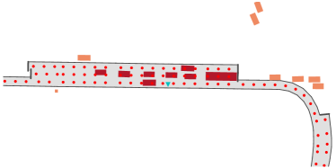
(a)  

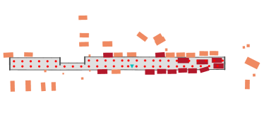
(b)  

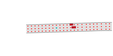
(c)  

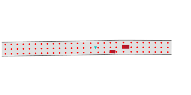
(d)  

Figure 7: BEV representation of scenes from the Argoverse dataset are shown in subfigure (a) and subfigure (b). Similar representation of scenes from the Carla simulated dataset are shown in subfigure (c) and subfigure (d). In all subfigures, the red dots represent the center of a grid and potential local goals, gray surfaces represent drivable lane surfaces, gray boundaries represent lane boundaries, red rectangles represent on lane NPC actors, orange rectangles represent off lane NPC actors, and the blue triangle represents the ego actor.

BEV Visualization.

fig. 7 shows visualizations of the BEV representation of scenes from the Argoverse dataset and the Carla simulator. The Drivable area is shown in gray with potential local goals shown as red dot. The Lane boundaries are shown in dark gray around the drivable area as static obstacles $B$. The actors that are on-lane are shown in red, and actors that are off-lane are shown in orange. Finally, since the BEV representation uses a ego-centered coordinate system so it is always the middle of the figure, shown in light blue triangle.

Appendix D Illustration of STI calculation using reachability.

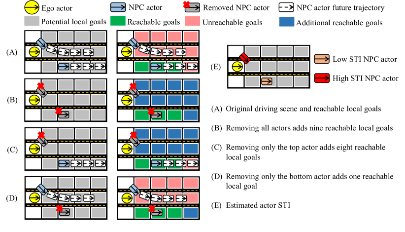
Figure 8: STI calculation using discretized drivable areas and reachability to the grids. Subfigure (A) shows STI calculation with all actors present, (B) shows STI calculation with all actors removed, (C) or (D) shows STI calculation with one of the actor removed, and (E) shows the relative actor STI in this scene.

fig. 8 illustrates the scene and actor STI calculation via discretized drivable areas and reachability (recall section 2.1 in the main paper) in a two NPC actors scene, in which one NPC actor cuts in front of the ego actor from the left and the other NPC actor travels straight in the right lane.

Starting with the original configuration as shown in fig. 8 (a), we first calculate the local goals’ reachability with all NPC actors present. After accounting for the NPC actors’ trajectories into the future and the ego actor’s dynamic capability, only three cells are reachable. Note that even though it appears that the bottom NPC actor occupies certain local goals in the bottom lane, those goals are in fact reachable by the ego actor as the bottom NPC actor will move ahead in the next $k$ (recall $k$ is the time budget) time steps.

Then, (B) calculates the reachability to the local goals with all NPC actors removed. After removing all NPC actors, all local goals are reachable by the ego actor. Compared to (A) the original setting, removing all actors increases driving flexibility by nine local goals. After reachability calculation of (A) and (B) we have sufficient information to calculate the scene STI using eq. 6.

To calculate STI for a particular actor $i$ via counterfactual reasoning actor $i$ is remove from the scene and the reachability is recalculated. Together with the reachability information on scene (A) and (B), we can then calculate the STI for $i$ using eq. 5. This is shown in (C) and (D) in fig. 8, with (C) removes the top actor, and (D) removes the bottom actor. Because the top actor resulted in a larger driving flexibility reduction–removing it increases driving flexibility by eight goals compared to one goal by removing the bottom actor—the top NPC actor’s STI is higher as illustrated in (E) in which only the current location of the actor is shown.

Appendix E NN-based Approximator Additional Details

E.1 Dataset generation

The input to the neural network based reachability approximator is a set of stacked $k$ bird-eye-view (BEV) images $\mathbf{I}_{t:t+k}$ and the vector $\mathbf{e}_{t}$ that contains the ego actor’s current state (see section 2.1). $\mathbf{I}_{t:t+k}=\{I_{t},I_{t+1},...,I_{t+k}\}$ can be constructed from the BEV representation $(G_{k},\mathbb{X}_{t:t+k},x_{t}^{ego},B)$, where $G_{k}$ is the set of potential goals, $\mathbb{X}_{t:t+k}$ is the set of actor states for all actors from $t$ to $t+k$, $x_{t}^{ego}$ is the current state of the ego actor, and $B$ is the set of static road boundaries (treated as static obstacles).

Let’s first take time step $t$ and generation of the BEV image $I_{t}$ as an example. Recall that the BEV representation $(G_{k},\mathbb{X}_{t:t+k},x_{t}^{ego},B)$ uses the ego-centered coordinate system and the goal is to convert such a representation in to a BEV binary image in which the drivable areas, such as open lane space, are labeled as 1, and the undrivable areas, such as those that are occupied by the NPC actors or out-of-lane, are labeled as 0.

Generating BEV binary images $\mathbf{I}_{t:t+k}$.

We first convert the ego-centered coordinate into image-coordinates, in terms of pixels. Following the convention of a 2D array representation, we set the direction from top to bottom as the positive x-direction, and from left to right as the positive y-direction, the origin of the image is at the top-left corner. Suppose we limit the view ranges of the x-direction to $[-R_{X},+R_{X}]$ and the y-direction to $[-R_{Y},+R_{Y}]$ in the ego-centered coordinates BEV representation, we can then generate a top-down abstract BEV visualization (it is abstact because the coordinates are continuous) of the BEV representation in terms of ego-centered coordinates, with the ego actor at the center and the positive y-direction (to the right of the visualization) being the forward direction. The visualization is only generated for the range between $[-R_{X},+R_{X}]$, and $[-R_{Y},+R_{Y}]$ and cuts off otherwise. In this visualization, areas that are part of the drivable lanes (i.e.,are not occupied by $\mathbb{X}_{t}$ or $B$) can be labeled as 1, and the rest 0. Suppose we denote this abstract visualization as $V_{t}$ then for each location $(X,Y)\in[-R_{X},+R_{X}]\times[-R_{Y},+R_{Y}]$

$$V_{t}(X,Y)=1\text{ if }(X,Y)\notin\mathbb{X}_{t}\land(X,Y)\notin B,\text{ else }V_{t}(X,Y)=0$$ (18)

We can then convert this abstract BEV visualization $V_{t}$ into a binary image $I_{t}$ by applying the transformation that maps ego-centered coordinates to image pixel coordinates. Suppose the input image $I_{t}$ is of size $H\times W$ then each pixel represents a distance in the x-direction of $\frac{2R_{X}}{H}$ meters, and distance in the y-direction of $\frac{2R_{Y}}{W}$ meters. The transform that maps ego-centered coordinates $(X,Y)$ to image pixel coordinates $(x,y)$ is defined as follows:

$$(x,y)=\left(\left\lfloor{\frac{X+R_{X}}{2R_{X}/H}}\right\rfloor,\left\lfloor{\frac{Y+R_{Y}}{2R_{Y}/W}}\right\rfloor\right)$$ (19)

To construct the BEV image for the future time steps, i.e., $I_{t+1}$ to $I_{t+k}$, we can simply replace the set of current actor states $\mathbb{X}_{t}$ with the state predictions for future time steps: $\mathbb{X}_{t+1}$, $\mathbb{X}_{t+2}$ etc., while other states the same. The $\mathbf{I}_{t:t+k}=\{I_{t},I_{t+1},...,I_{t+k}\}$ can then be constructed from the set of BEV images just generated.

Labeling reachability indicator vector $\mathbf{r}_{k}^{*}$.

The output of the NN-based reachability approximator is (see eq. 7) is a reachability indicator vector $\mathbf{r}_{k}$ which each element indicating a location on the BEV image as reachable or not reachable. Since the neural network’s output size is fixed, we choose to discretize the entire BEV image into grids instead of using the original discretized grids of drivable areas in which the number of grids may vary. Below we describe the process of generating the ground truth label $\mathbf{r}_{k}^{*}$ for training and evaluation.

Suppose each grid is of size $a\times b$ pixels in the BEV image space. A grid of size $a\times b$ in the image space is equivalent of a grid of size $\frac{2bR_{Y}}{W}$ meters in the y-direction, and $\frac{2aR_{X}}{H}$ meters in the x-direction in the ego-centered coordinate system (used by $V_{t}$). Given a BEV image size of $H\times W$, there are in total $\left\lfloor\frac{H}{a}\right\rfloor\times\left\lfloor\frac{W}{b}\right\rfloor$ grids. Notice that goals are only in the forward direction as we assume the ego actor cannot travel backward, so we can remove the grids for the left half of the BEV image because they contain no goals. $\mathbf{r}_{k}^{*}$ can then be constructed from a vector of all zeros of size $\left\lfloor\frac{H}{a}\right\rfloor\times\left\lfloor\frac{W}{2b}\right\rfloor$, then setting the elements which overlaps with a reachable goal $g_{k}\in R_{k}$ to 1, where $R_{k}$ is the output of eq. 17:

$$\mathbf{r}_{k}^{*}[i]=1\text{ if }i^{th}\text{ grid contains a reachable goal }g_{k}\in R_{k}\text{ in the image space, else 0.}$$ (20)

We choose $H=128$px, $W=512$px, $R_{X}=17.5$m, $R_{Y}=70$m, $a=11$px, $b=20$px for all the experiments. The training dataset is generated from Argoverse training dataset which consists of $\sim 7800$ datapoints. The testing dataset is generated from the Argoverse validation dataset which consists of $\sim 930$ datapoints. Furthermore, we perform a 80%-20% split on the training data set for train-validation during the training procedure.

Dataset visualization.

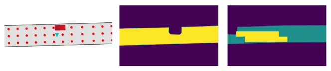
Figure 9: NN-based reachability approximator training and evaluation dataset visualization. The left subfigure shows the BEV representation of a scene. The middle subfigure shows a part of the input data $I_{t}$ based on the BEV representation. The right subfigure visualizes the label $\mathbf{r}_{t}$. In the label visualization (the right subfigure), dark areas are undrivable ares, greenish-blue areas are drivable lanes, and the yellow grids represents reachable grids (elements of $\mathbf{r}_{t}$ whose values are 1) in the image space.

fig. 9 shows the visualization of the generated dataset. The left subfigure shows the original BEV representation of the scene, with the red-dots being the potential local goals, red blocks being an NPC actor, and drivable areas in gray. The middle subfigure shows the binary BEV image $I_{t}\in\mathbf{I}_{t:t+k}$ as part of the input to the model, with bright areas being the drivable areas and dark areas being the undrivable areas; notice that the NPC actor is part of the undrivable area. The right subfigure visualizes the drivable (in greenish-blue), non-drivable areas (dark), and reachable grids indicated by $\mathbf{r}_{k}$ (yellow). The drivable areas that are not reachable by the ego actor due to the presence of the NPC actor aren’t highlighted in yellow.

E.2 NN-based reachability approximator architecture

Layer(s)	Input dim	Output dim
Fully connected + ReLU	$\mathbf{e}_{t}$: $(1\times 5)$	$(1,H,W)$
Concatenate [$\mathbf{I}_{t:t+k}$, $\mathbf{e}_{t}$]	$Concat([(k+1,H,W)$, $(1,H,W)])$	$(k+2,H,W)$
ResNet-34 backbone + ReLU	$(k+2,H,W)$	$(512,H//32,W//32)$
Fully connected + ReLU	$(512\times H//32\times W//32)$	$(32\times\left\lfloor\frac{H}{a}\right\rfloor\times\left\lfloor\frac{W}{2b}\right\rfloor)$
Fully connected + ReLU	$(32\times\left\lfloor\frac{H}{a}\right\rfloor\times\left\lfloor\frac{W}{2b}\right\rfloor)$	$(16\times\left\lfloor\frac{H}{a}\right\rfloor\times\left\lfloor\frac{W}{2b}\right\rfloor)$
Conv + Sigmoid + flatten	$(16,\left\lfloor\frac{H}{a}\right\rfloor,\left\lfloor\frac{W}{2b}\right\rfloor)$	$(\left\lfloor\frac{H}{a}\right\rfloor\times\left\lfloor\frac{W}{2b}\right\rfloor)$

Table 3: NN-based reachability approximator model input, architecture, and output.

The model of the NN-based reachability approximator uses the Resnet-34 as a backbone and a customized output head to output the reachability indicator vector. table 3 lists the input, output, and the model architecture. The inputs of the model are $\mathbf{I}_{t:t+k}$ and $\mathbf{e}_{t}$ (we pre-process $\mathbf{e}_{t}$ using a fully connected layer to transform it into same shape of the input BEV images as an additional channel), the output of the model is a vector of size $\left\lfloor\frac{H}{a}\right\rfloor\times\left\lfloor\frac{W}{2b}\right\rfloor$. We omit the mini-batch dimension, and the usage of $flatten$ when appropriate for better clarity.

Appendix F SMC Additional Details

F.1 Mutated scenarios hyperparameters

The 1000 mutated scenarios are generated based on the cut in safety-critical scenario typology, as described in section 4.1, by varying multiple adjustable hyperparameters as follows.

1. Distance traveled before cut in: This parameter specifies the distance that the NPC actor travels before starting to cut in. The lower the value, the sooner the cut in happens after the NPC actor passes the ego actor, the more severe the criticality. We vary this parameter value in the range of $[10,20)$, with an increment of 1.

2. Distance traveled during lane change: This parameter specifies the distance that the NPC actor travels during the cut in. The lower the value, the steeper the cut in angle, the more severe the criticality, and vise versa. We vary this parameter value in the range of $[6,16)$, with an increment of 1.

3. Lane change speed: This parameter specifies the speed of the NPC actor during the cut in. The lower the value, the lower the cut in speed, the longer it takes to complete the cut in, and vise versa. We vary this parameter value in the range of $[9,19)$, with an increment of 1.

We then generate scenarios using all combinations of these three hyperparameters, which in term resulted in 1000 mutations of the base scenario. For each run of the LBC agent on these mutated scenarios, we collect the simulator data on actors and the map information which results in a dataset similar to the Argoverse dataset. This dataset is referred to as mutated scenarios dataset.

We can convert this dataset using the same method outlined in section 2.1 and section E.1 in to the training and evaluation dataset for the NN-based reachability approximator to be used in simulator environment. The training dataset is generated from 80% of the 1000 scenarios which consists of $\sim 340$K datapoints. The testing dataset is generated from the rest 20% which consists of $\sim 83$K datapoints. Additionally, we perform a 80%-20% split on the training data set for validation during the training procedure.

Training and evaluating the SMC.

We also use one (the scenario with the median value of individual hyperparameter ranges) of these 1000 mutated scenarios to train the SMC and learn a mitigation policy (section 4.2.2). We then evaluate this policy using all of the 1000 mutated scenarios to assess the generalizability of the learned policy. The result in section 5.3 shows that the policy is generalizable to different level of safety criticality of the similar scenario typology as SMC reduces the accident rate significantly.

F.2 RL Reward function

eq. 10 defines a general reward formulation as a multi-parts weight sum to encode the trade-offs of mitigation actions. This subsection defines the various terms used in this reward function. In general, the reward function should encourage mitigation in high STI situation, but discourage mitigation that affects normal driving in low STI situation.

1. STI: The value of the scene STI evaluated per simulation time step. The term $(1-{STI})$ encourages low STI and discourage high STI. During our implementation, we do find that this term dominates and continue to provide large positive rewards even if the mitigation action like emergency braking is activated continuously, as long as the scene risk is 0 or low. This lead to a mode collapse as the ego vehicle continues to receive reward even if it is stationary (holding the emergency brake). We reduce this effect by multiplying this term with the speed factor $v_{f}$ (described as part of the $r_{pc}$): $(1-{STI})v_{f}$ so that no rewards are given if the ego actor is stationary.

2. $r_{pc}$: The path-completion reward term describes the reward for completing the path.

   $$r_{pa}=(\mathbf{u}_{ego}\cdot\mathbf{u}_{goal})v_{f}$$ (21)

   $$v_{f}=\frac{\|\mathbf{d}_{ego}\|}{d_{expected}}$$ (22)

   where $\mathbf{u}_{ego}$ is the unit vector of the ego actor’s traveling direction, $\mathbf{u}_{goal}$ is the unit vector of the goal/next-planned waypoint direction, $\|\mathbf{d}_{ego}\|$ is the distance covered by ego actor per time step, and $d_{expected}$ is the expected coverage if the road is NPC actor free. $r_{pc}$ encourages the actor to travel in the planned direction with the expected speed, and discourages large deviation from the planned route or the expected speed.

3. $p_{am}$: The active-mitigation penalty term penalizes the activation of the mitigation action in general because mitigation actions can change the dynamic of the ego actor drastically, resulting in passenger discomfort and even panics. This term can be a constant that applies whenever mitigation is activated, and otherwise zero, we do found that introduces such a term lead to discontinuity in the reward function which affects the Q-function’s convergence, so a smoother function is needed. As a result we set this term to zero in our experiments.

4. $r_{comfort}$: Given that the ego agents used/evaluated in this paper chen2019lbc ; pmlr-v119-filos20a do not account for comfort explicitly, we also decided to not account for comfort to reduce the time for training. However, the reward model can be extended to account for comfort by using equation eq. 23. In real world modeling comfort is important because an aggressive mitigation policy can cause unnecessary discomforts. Comfort is commonly characterized as the rate of change in acceleration so one way to define $r_{comfort}$ is as follows, where $a$ is the acceleration:

   $$r_{comfort}=-(j_{lat}+j_{long}),j=\frac{da}{dt}$$ (23)

F.3 SMC model architecture

As specified in section 4.2.2 the SMC’s Q-value function uses a similar architecture as the LBC agent’s Sensorimotor model chen2019lbc with the only changes being the input and the output format. We choose this design as the SMC consumes similar input as the original ego actor’s input to more efficiently reuse information and reduce complexity.

We change the original input format, a $10$-channel 3D feature maps that consists of 3 RGB images from 3 front facing cameras and 1 target heatmap, to a $16$-channel 3D feature maps. Instead of using 3 RGB images as part of the input, we convert these 3 RGB images into 3 grayscale images. In addition, we collect such feature maps for 4 consecutive simulation time step to capture the temporal information, so the resulting feature maps is consists of 16 channels, with the first 12 channels being the grayscale images (3 cameras ×4 time steps), and 4 target heatmap (1 heatmap per time step).

The output format of the original Sensorimotor model is a $4\times 2$ vector that contains $4$ local waypoints to follow. We change this format and now the output equals to the dimension of the action space with each element specify the Q-value of that action; in our case, the output is $1\times 2$.

We refer the reader to chen2019lbc for more details of the architecture used.

Appendix G Compute Hardware and Compute Hours

G.1 Hardware specifications

We train and evaluate the NN-based reachability approximator and the RL-based SMC on a system with AMD Ryzen 9 3950X CPU, 64 GB of system memory, and a RTX 3090 TI with 24 GB of video memory. For training and evaluation dataset label generation and dataset STI characterization using the FOT planner based STI evaluator, a more powerful machine with AMD Ryzen Threadripper 3990X CPU and 128 GB of system memory is used to reduce computation time.

G.2 Compute hours

The NN-based approximator training and evaluation dataset generation from the $Arogoverse$ real-world dataset takes 25 CPU hours using the FOT planner based STI evaluator to generate label. The generation of dataset from the 1000 mutated scenarios takes 25 + 27 CPU hours, with the first 25 hours used for running and recording all 1000 mutated scenarios using the LBC agent, and the next 27 hours for label generation using the FOT planner based STI evaluator. Training of the NN-based reachability approximator for 500 epochs requires 9 hours of GPU time on the mutated scenarios dataset and 7 hours of GPU time on the Argoverse dataset. The evaluation of NN-based reachability approximator on real world dataset consumes 1 hours of GPU time, while the evaluation on the simulated dataset consumes 2 hours due to more data. Training of the RL-based SMC for 100 episodes requires roughly 500 minutes or 8.3 hours, with each episode consumes approximately 5 minutes of wall clock time. The evaluation of the SMC on the 1000 mutated scenarios takes around 33 hours with each run finishes in 2 minutes. For baseline comparison, evaluation of the LBC agent on the 1000 mutated scenarios takes around the same time as with SMC enabled. For comparison with the RIP agent, evaluation on the 1000 mutated scenarios takes around 50 hours, with each run finishes in 3 minutes.

Appendix H Hyperparameters

We list the hyperparameters used in this work below.

1. FOT planner based STI calculation with BEV representation (sections 2.1 and C).

   • Time budget (Look forward time): $3$ seconds is equivalent to $k=30$ as all data (real and simulated) are collected at 10 Hz.

   • Distance budget (Look forward distance): $d_{max}=120$ meters, distance threshold for potential local goals is $d_{thres}=\max(d,d_{max})$, where $d$ is specified in eq. 15.

   • Lane width (grid width): $w=3.7$ meters for Argoverse dataset; width varies with mutated scenarios dataset dataset based on actual simulated lane width.

   • Grid distance (grid length): $l=4.5$ meters for both Argoverse dataset and mutated scenarios dataset.

   • Minimum distance to static obstacles (lane boundaries): 0.1 meters.

   • Minimum distance to dynamic obstacles (NPC actors): 1.5 meters.

   • FOT planner hyperparameters based on typical consumer vehicle.

     1. Maximum speed: 100 $km/h$, 27.7 $m/s$.

     2. Maximum acceleration: 4.0 $m/s^{2}$.

     3. Maximum turning curvature: 0.2 $m^{-1}$.

2. NN-based reachability approximation.

   • Reachability approximation dataset generation.

     1. All hyperparameters used in FOT planner based STI calculation with BEV representation for reachability label generation.

     2. BEV image height: $H=128$ pixels.

     3. BEV image width: $W=512$ pixels.

     4. X-axis view range (x-axis): $R_{X}=17.5$ meters.

     5. Y-axis view range (y-axis): $R_{Y}=70.0$ meters.

     6. # of pixels in the reachability grid in the X-direction: $a=11$ pixels.

     7. # of pixels in the reachability grid in the Y-direction: $b=20$ pixels.

   • Model hyperparameters: The hyperparameters for the NN-based reachability approximator’s neural network model can be derived from the shape of the input and output specified in table 3.

   • Training and validation.

     1. Adam optimizer learning rate: $1\text{\times}{10}^{-5}$.

     2. Adam optimizer weight decay: $0.99$.

     3. Number of epoch: $500$.

3. RL-based SMC for mitigation.

   • Mutated scenarios dataset generation: See section F.1 for hyperparameters used.

   • Model hyperparameters: The SMC Q-value model’s neural network model are specified in section F.3 and chen2019lbc .

   • Training and evaluation.

     1. Adam optimizer learning rate: $1\text{\times}{10}^{-5}$.

     2. Adam optimizer weight decay: $0.9999$.

     3. RL reward decay: $0.99$.

     4. Number of episodes: $100$.

References

- (1) S.-T. Chen, C. Cornelius, J. Martin, and D. H. P. Chau, “Shapeshifter: Robust physical adversarial attack on faster r-cnn object detector,” in Joint European Conference on Machine Learning and Knowledge Discovery in Databases, pp. 52–68, Springer, 2018.
- (2) S. Jha, S. Cui, S. Banerjee, J. Cyriac, T. Tsai, Z. Kalbarczyk, and R. K. Iyer, “ML-driven malware that targets AV safety,” in 2020 50th Annual IEEE/IFIP International Conference on Dependable Systems and Networks (DSN), pp. 113–124, IEEE, 2020.
- (3) Y. Jia, Y. Lu, J. Shen, Q. A. Chen, H. Chen, Z. Zhong, and T. Wei, “Fooling detection alone is not enough: Adversarial attack against multiple object tracking,” in ICLR 2020 : Eighth International Conference on Learning Representations", 2020.
- (4) S. S. Banerjee, S. Jha, J. Cyriac, Z. T. Kalbarczyk, and R. K. Iyer, “Hands off the wheel in autonomous vehicles?: A systems perspective on over a million miles of field data,” in 2018 48th Annual IEEE/IFIP International Conference on Dependable Systems and Networks (DSN), pp. 586–597, 2018.
- (5) S. Alvarez, “Research group demos why Tesla Autopilot could crash into a stationary vehicle.” https://www.teslarati.com/tesla-research-group-autopilot-crash-demo/, June 2018.
- (6) T.S., “Why Uber’s self-driving car killed a pedestrian.” The Economist May 29, 2018 https://www.economist.com/the-economist-explains/2018/05/29/why-ubers-self-driving-car-killed-a-pedestrian.
- (7) D. Chen, B. Zhou, V. Koltun, and P. Krähenbühl, “Learning by cheating,” in Proceedings of the Conference on Robot Learning (L. P. Kaelbling, D. Kragic, and K. Sugiura, eds.), vol. 100 of Proceedings of Machine Learning Research, pp. 66–75, PMLR, 30 Oct–01 Nov 2020.
- (8) “Apollo Open Platform.” http://apollo.auto. Accessed: 2018-09-02.
- (9) A. Filos, P. Tigkas, R. Mcallister, N. Rhinehart, S. Levine, and Y. Gal, “Can autonomous vehicles identify, recover from, and adapt to distribution shifts?,” in Proceedings of the 37th International Conference on Machine Learning (H. D. III and A. Singh, eds.), vol. 119 of Proceedings of Machine Learning Research, pp. 3145–3153, PMLR, 13–18 Jul 2020.
- (10) J. Philion, A. Kar, and S. Fidler, “Learning to evaluate perception models using planner-centric metrics,” in Proceedings of the IEEE/CVF Conference on Computer Vision and Pattern Recognition (CVPR), June 2020.
- (11) S. M. LaValle et al., “Rapidly-exploring random trees: A new tool for path planning,” 1998.
- (12) M. Werling, J. Ziegler, S. Kammel, and S. Thrun, “Optimal trajectory generation for dynamic street scenarios in a Frenét frame,” in 2010 IEEE International Conference on Robotics and Automation, pp. 987–993, 2010.
- (13) M.-F. Chang, J. Lambert, P. Sangkloy, J. Singh, S. Bak, A. Hartnett, D. Wang, P. Carr, S. Lucey, D. Ramanan, and J. Hays, “Argoverse: 3d tracking and forecasting with rich maps,” in Proceedings of the IEEE/CVF Conference on Computer Vision and Pattern Recognition (CVPR), June 2019. Dataset: CC BY-NC-SA 4.0 License, tools and code: MIT License.
- (14) A. Piazzoni, J. Cherian, M. Slavik, and J. Dauwels, “Modeling perception errors towards robust decision making in autonomous vehicles,” arXiv preprint arXiv:2001.11695, 2020.
- (15) N. David, L. Hon-Leung, N. Julia, and W. Yizhou, “An introduction to the safety force field.” https://www.nvidia.com/content/dam/en-zz/Solutions/self-driving-cars/safety-force-field/an-introduction-to-the-safety-force-field-updated.pdf, 2019.
- (16) S. Shalev-Shwartz, S. Shammah, and A. Shashua, “On a formal model of safe and scalable self-driving cars,” arXiv preprint arXiv:1708.06374, 2017.
- (17) D. Dolgov, S. Thrun, M. Montemerlo, and J. Diebel, “Practical search techniques in path planning for autonomous driving,” Ann Arbor, vol. 1001, no. 48105, pp. 18–80, 2008.
- (18) A. Dosovitskiy, G. Ros, F. Codevilla, A. Lopez, and V. Koltun, “CARLA: An open urban driving simulator,” in Proceedings of the 1st Annual Conference on Robot Learning (S. Levine, V. Vanhoucke, and K. Goldberg, eds.), vol. 78 of Proceedings of Machine Learning Research, pp. 1–16, PMLR, 13–15 Nov 2017.
- (19) LG Electronics, “LGSVL simulator.” https://www.lgsvlsimulator.com/, 2018.
- (20) W. G. Najm, J. D. Smith, M. Yanagisawa, et al., “Pre-crash scenario typology for crash avoidance research,” tech. rep., United States. National Highway Traffic Safety Administration, 2007.
- (21) “ResNet 34.” https://models.roboflow.com/classification/resnet34.
- (22) D. P. Kingma and J. Ba, “Adam: A method for stochastic optimization,” arXiv preprint arXiv:1412.6980, 2014.
- (23) V. Mnih, K. Kavukcuoglu, D. Silver, A. Graves, I. Antonoglou, D. Wierstra, and M. Riedmiller, “Playing atari with deep reinforcement learning,” arXiv preprint arXiv:1312.5602, 2013.
- (24) H. van Hasselt, A. Guez, and D. Silver, “Deep reinforcement learning with double q-learning,” CoRR, vol. abs/1509.06461, 2015.
- (25) N. Rhinehart, K. M. Kitani, and P. Vernaza, “R2p2: A reparameterized pushforward policy for diverse, precise generative path forecasting,” in Proceedings of the European Conference on Computer Vision (ECCV), September 2018.
- (26) K. Viswanadha, F. Indaheng, J. Wong, E. Kim, E. Kalvan, Y. Pant, D. J. Fremont, and S. A. Seshia, “Addressing the ieee av test challenge with scenic and verifai,” in 2021 IEEE International Conference on Artificial Intelligence Testing (AITest), pp. 136–142, 2021.
- (27) G. Li, Y. Li, S. Jha, T. Tsai, M. Sullivan, S. K. S. Hari, Z. Kalbarczyk, and R. Iyer, “Av-fuzzer: Finding safety violations in autonomous driving systems,” in 2020 IEEE 31st International Symposium on Software Reliability Engineering (ISSRE), pp. 25–36, 2020.
- (28) J. F. Fisac, E. Bronstein, E. Stefansson, D. Sadigh, S. S. Sastry, and A. D. Dragan, “Hierarchical game-theoretic planning for autonomous vehicles,” in 2019 International Conference on Robotics and Automation (ICRA), pp. 9590–9596, IEEE, 2019.
- (29) I. Gog, S. Kalra, P. Schafhalter, M. A. Wright, J. E. Gonzalez, and I. Stoica, “Pylot: A modular platform for exploring latency-accuracy tradeoffs in autonomous vehicles,” 2021.
- (30) M. Li, Y.-X. Wang, and D. Ramanan, “Towards streaming perception,” in European Conference on Computer Vision, pp. 473–488, Springer, 2020.
- (31) J. Redmon and A. Farhadi, “YOLOv3: An incremental improvement,” arXiv preprint arXiv:1804.02767, 2018.
- (32) G. Welch, G. Bishop, et al., An introduction to the Kalman filter. Los Angeles, CA, 1995.