Lattice QCD calculation of light sterile neutrino contribution
in $0\nu 2\beta$ decay

Abstract

We present a lattice QCD study of the neutrinoless double beta decay involving light sterile neutrinos. The calculation is performed at physical pion mass using five gauge ensembles generated with $2+1$-flavor domain wall fermions. We obtain the low-energy constants $g_{\text{LR}}^{\pi\pi}(m_{\nu})$ with the neutrino mass $m_{\nu}$ from $0$ GeV to $3$ GeV. The lattice results are reasonably consistent with the previous interpolation method Dekens et al. (2020) with a $\sim 20$% deviation at small $m_{\nu}$. We provide an explanation on the discrepancy at vanishing neutrino mass. At large $m_{\nu}$, a good consistency between our results and the previous lattice determination of $g_{4}^{\pi\pi}(\mu)$ Nicholson et al. (2018) is found at $\mu=m_{\nu}=3$ GeV.

I Introduction

Observation of new physics beyond the Standard Model (BSM) is one of the most central themes in particle physics. It is a milestone that the neutrino oscillations are observed and the neutrinos are demonstrated as massive particles. To further determine the absolute mass of the neutrinos and verify whether the neutrinos are Dirac or Majorana fermions, neutrinoless double beta ($0\nu 2\beta$) decay experiments Agostini et al. (2019); Gando et al. (2016); Alduino et al. (2018); Albert et al. (2018); Azzolini et al. (2018); Alvis et al. (2019); Agostini et al. (2020); Armengaud et al. (2021); Adams et al. (2022); Abe et al. (2022) provide an excellent probe. In the framework of effective field theory (EFT), a roadmap to reach the theoretical determination of the $0\nu 2\beta$ decay amplitude is laid out through a path from the BSM scenarios at high energy towards the nuclear many-body theories at low energy Cirigliano et al. (2022). At the energy of $O(1)$ GeV - $O(100)$ MeV, chiral perturbation theory ($\chi$PT) and its extension to the multi-nucleon sector, namely chiral EFT, serve as a bridge to connect quark-level theories and nuclear-level theories Cirigliano et al. (2017a, b, 2018a); Pastore et al. (2018); Cirigliano et al. (2018b, c, 2019); Dekens et al. (2020); Cirigliano et al. (2021a, b). To construct the hadronic operators, it requires the non-perturbative inputs of the low-energy couplings from lattice QCD Cirigliano et al. (2020).

In recent years lattice QCD calculations have successfully provided the hadronic matrix elements for double neutrino double beta decay in the nucleon sector Shanahan et al. (2017); Tiburzi et al. (2017) and $0\nu 2\beta$ matrix elements in the pion sector including both long-distance contributions via Majorana neutrino exchange Feng et al. (2019); Tuo et al. (2019); Detmold and Murphy (2020) and short-distance contributions via dim-9 operators Nicholson et al. (2018). The approaches to match the lattice matrix elements from finite volume to the double beta decay amplitudes in the infinite volume are also proposed Feng et al. (2021); Davoudi and Kadam (2020, 2021, 2022).

Among various BSM models, the inclusion of additional sterile neutrinos presents an important class of the extension of the Standard Model, as it can be used to explain the matter/antimatter asymmetry via low-scale leptogenesis Akhmedov et al. (1998); Asaka et al. (2005); Asaka and Shaposhnikov (2005); Shaposhnikov (2007); Canetti et al. (2013); Hernández et al. (2016); Ghiglieri and Laine (2017). If these neutrinos are Majorana particles, they can mediate and influence the $0\nu 2\beta$ decay rates. Understanding the impact of massive sterile neutrinos can help $0\nu 2\beta$ experiments provide more constraints on neutrino mass scenarios. As such, the EFT description of the $0\nu 2\beta$ decay has been extended to include the option of light sterile neutrinos Dekens et al. (2020). Using an effective interpolation method it is found that the decay amplitudes peak at the neutrino mass in a range from few hundreds MeV to few GeV. The exact location of peak would rely on the input of the underlying operators. The determination of them is highly non-trivial due to non-perturbative nature of QCD. As a consequence, it brings in sizable uncertainties at the order-of-magnitude level, which are dominated by the low-energy constants (LECs). It motivates our lattice QCD study of the non-trivial neutrino mass dependence of LECs, which is reported here.

II Theoretical background

Here we follow the systematic EFT approach Dekens et al. (2020) to add the massive sterile neutrinos in $0\nu 2\beta$ decay. At the energy above the electroweak scale $\Lambda_{\text{EW}}$, the SM is extended with sterile neutrinos in the framework of SMEFT del Aguila et al. (2009); Cirigliano et al. (2013); Asaka et al. (2016); Liao and Ma (2017, 2019); Liao et al. (2020); Liao and Ma (2020) and the higher-dimensional operators are included when the non-neutrino states heavier than $\Lambda_{\text{EW}}$ are integrated out. To describe physics at or below $\Lambda_{\text{EW}}$, it proceeds in two different ways depending on the size of the neutrino mass $m_{\nu}$. For $\Lambda_{\chi}<m_{\nu}<\Lambda_{\text{EW}}$ where $\Lambda_{\chi}$ is chiral symmetry breaking scale, the sterile neutrinos are integrated out and effective local operators are produced. For $m_{\nu}<\Lambda_{\chi}$, the neutrino remains an active degree of freedom propagating at the hadronic scale. In this case, one needs to obtain the $0\nu 2\beta$ transition operators induced by light sterile neutrino in the framework of chiral EFT. The relevant nuclear matrix elements (NMEs) and the LECs in the chiral Lagrangian are all non-perturbative, and thus their dependence on the mass of the sterile neutrinos is poorly known. In Ref. Dekens et al. (2020) naive interpolation formulae grounded in QCD and $\chi$PT are proposed to connect the regimes with $m_{\nu}\ll\Lambda_{\chi}$ and $m_{\nu}\gg\Lambda_{\chi}$. Further improvements can be made if the relevant pion, nucleon and two-nucleon matrix elements are calculated and the LECs are extracted using non-perturbative techniques such as lattice QCD. As the last step, the NMEs and the LECs are used to estimate the $0\nu 2\beta$ half-lives. Both the uncertainties on the NMEs and LECs play a significant role in the determination of the $0\nu 2\beta$ half-lives and hence the comparison with the experiments.

As mentioned above, lattice QCD can provide useful LECs for the construction of hadronic operators defined in $\chi$PT and chiral EFT. For simplicity, at low energy we discuss the scenario involving one neutrino mass eigenstate with mass $m_{\nu}$ which couples to left-handed electrons and to both right- and left-handed quark vector currents. Namely, the dim-6 operators describing the four-fermion interaction are introduced as

$$\mathcal{L}^{(6)}=\frac{2G_{F}}{\sqrt{2}}\left[C_{\mathrm{VLL}}^{(6)}\bar{u}_{L}\gamma^{\mu}d_{L}\bar{e}_{L}\gamma_{\mu}\nu+C_{\mathrm{VRL}}^{(6)}\bar{u}_{R}\gamma^{\mu}d_{R}\bar{e}_{L}\gamma_{\mu}\nu\right]+\text{h.c.},$$ (1)

where $G_{F}$ is Fermi constant, $u,d$ are quark fields and $e,\nu$ are electron and neutrino fields. Although only one neutrino mass eigenstate is involved here, the operator can be easily extended to include more mass eigenstates. Here $C_{\mathrm{VLL}}^{(6)}$ and $C_{\mathrm{VRL}}^{(6)}$ are Wilson coefficients which factorize information of underlying short-distance contribution of the BSM scenarios. Note that we do not include the scalar and tensor operators as well as higher dimensional operators. Thus, up to the Wilson coefficients, one can view Eq. (1) as a simple extension of Standard Model to include the coupling of neutrino to right-handed quark current.

The $0\nu 2\beta$ decay involves the double current insertions with the vector couplings $C_{\mathrm{VLL,VRL}}^{(6)}$. The general amplitude in the hadronic sector is given by

$$\left\langle h_{f}e_{1}e_{2}\left|\frac{i}{2!}\int d^{4}x\,T\left\{\mathcal{L}^{(6)}(x)\mathcal{L}^{(6)}(0)\right\}\right|h_{i}\right\rangle,$$ (2)

where $h_{i,f}$ are hadronic states. The decay amplitude at the quark level shall be matched to the one at the hadronic level using chiral Lagrangian. At leading order, both the Lagrangian $\mathcal{L}_{\pi\pi}$ describing the $\pi^{-}\to\pi^{+}ee$ transition and $\mathcal{L}_{NN}$ appearing in the nucleon-nucleon sector are important. Eq. (2) does not induce $\pi N$ couplings at leading order and thus we neglect them. The pionic Lagrangian is given by

$$\mathcal{L}_{\pi\pi}=2G_{F}^{2}F_{\pi}^{2}C_{\mathrm{VLL}}^{(6)}C_{\mathrm{VRL}}^{(6)}m_{\nu}g_{\mathrm{LR}}^{\pi\pi}\left(m_{\nu}\right)\mathrm{Tr}\left[\mathcal{Q}_{L}\mathcal{Q}_{R}\right]\bar{e}_{L}e_{L}^{c},$$ (3)

with $\mathcal{Q}_{L}=u^{\dagger}\tau^{+}u$, $\mathcal{Q}_{R}=u\tau^{+}u^{\dagger}$ and $\tau^{\pm}=(\tau_{1}\pm i\tau_{2})/2$, where $\tau_{i}$ are the Pauli matrices and $u$ is a $2\times 2$ matrix containing the pion fields and transforming as $u\to LuK^{\dagger}=KuR^{\dagger}$ under $SU(2)_{L}\times SU(2)_{R}$ transformations. Here $F_{\pi}$ is a pion decay constant. The terms associated with $(C_{\mathrm{VLL}}^{(6)})^{2}$ and $(C_{\mathrm{VRL}}^{(6)})^{2}$ produce the LEC $g_{\nu}^{\pi\pi}(m_{\nu})$, but are considered as higher-order contributions and thus neglected. The remaining $C_{\mathrm{VLL}}^{(6)}C_{\mathrm{VRL}}^{(6)}$ term contains the LEC $g_{\mathrm{LR}}^{\pi\pi}(m_{\nu})$, which is the main objective of this work. For the nucleonic Lagrangian $\mathcal{L}_{NN}$ which contains the LECs $g_{\mathrm{LR}}^{NN}(m_{\nu})$ and $g_{\mathrm{\nu}}^{NN}(m_{\nu})$, we leave it for the future study.

Considering the similarity between the exchange of the neutrinos in $0\nu 2\beta$ decay and the exchange of photons in the electromagnetic correction to the pion mass, $g_{\mathrm{LR}}^{\pi\pi}(m_{\nu})$ at $m_{\nu}=0$ can be approximated by Dekens et al. (2020)

$$g_{\text{LR}}^{\pi\pi}(m_{\nu}=0)\approx\frac{m_{\pi^{\pm}}^{2}-m_{\pi_{0}}^{2}}{2e^{2}}\approx 0.8F_{\pi}^{2}.$$ (4)

On the other hand, when the neutrino mass significantly exceed the scale $\Lambda_{\chi}$, the operator product of $\mathcal{L}^{(6)}$ in Eq. (2) will induce dimension-9 operators involving four quark and two lepton fields, namely $O_{4}=\bar{q}^{\alpha}_{L}\gamma_{\mu}\tau^{+}q_{L}^{\alpha}\,\bar{q}_{R}^{\beta}\gamma^{\mu}\tau^{+}q^{\beta}_{R}$ and its color-mixing pattern $O_{5}=\bar{q}^{\alpha}_{L}\gamma_{\mu}\tau^{+}q_{L}^{\beta}\,\bar{q}_{R}^{\beta}\gamma^{\mu}\tau^{+}q^{\alpha}_{R}$ with $\alpha$, $\beta$ color indices. The pion matrix elements involving $O_{4,5}$ can be used to extract the additional LECs $g_{4,5}^{\pi\pi}(\mu)$ through a leading-order $\chi$PT formula

$$g_{4,5}^{\pi\pi}(\mu)=\frac{1}{F_{\pi}^{2}}\langle\pi|O_{4,5}(\mu)|\pi\rangle.$$ (5)

Thus one can match $g_{\text{LR}}^{\pi\pi}(m_{\nu})$ at $m_{\nu}\gg\Lambda_{\chi}$ to $g_{4,5}^{\pi\pi}(\mu)$ as

$$g_{\text{LR}}^{\pi\pi}(m_{\nu})=C_{4}(m_{\nu},\mu)g_{4}^{\pi\pi}(\mu)+C_{5}(m_{\nu},\mu)g_{5}^{\pi\pi}(\mu),$$ (6)

where $C_{4,5}$ are the matching coefficients. Setting $\mu=m_{\nu}$, one has $C_{4}(m_{\nu},\mu)=-\frac{F_{\pi}^{2}}{4m_{\nu}^{2}}+\mathcal{O}(\alpha_{s})$ and $C_{5}(m_{\nu},\mu)=\mathcal{O}(\alpha_{s})$. The renormalization group equation (RGE) of $g_{4,5}^{\pi\pi}$ yields Dekens et al. (2020)

$$\frac{d}{d\ln\mu}\left(\begin{array}[]{l}g_{4}^{\pi\pi}\\ g_{5}^{\pi\pi}\end{array}\right)=-\frac{\alpha_{s}}{4\pi}\left(\begin{array}[]{cc}6/N_{c}&0\\ -6&-12C_{F}\end{array}\right)^{T}\left(\begin{array}[]{l}g_{4}^{\pi\pi}\\ g_{5}^{\pi\pi}\end{array}\right).$$ (7)

Using the direct lattice QCD calculation of $\langle\pi|O_{4,5}(\mu)|\pi\rangle$ Nicholson et al. (2018) at $\mu=3$ GeV as input, one obtains $g_{4}^{\pi\pi}(\mu)$ at $\mu=2$ GeV Dekens et al. (2020)

$$g_{4}^{\pi\pi}(\text{2 GeV})=-1.9(2)\text{ GeV}^{2},\quad g_{5}^{\pi\pi}(\text{2 GeV})=-8.0(6)\text{ GeV}^{2}.$$ (8)

In this work we plan to perform a direct lattice QCD calculation of $g_{\text{LR}}^{\pi\pi}(m_{\nu})$ in the range of 0 GeV $\leq m_{\nu}\leq 3$ GeV. The choice of $m_{\nu}$ allows us to perform a consistency check of Eq. (4) at $m_{\nu}=0$ and the previous lattice results of $g_{4}^{\pi\pi}(\mu)$ at $\mu=3$ GeV Nicholson et al. (2018) by assuming $g_{\text{LR}}^{\pi\pi}(m_{\nu})\simeq-\frac{F_{\pi}^{2}}{4m_{\nu}^{2}}g_{4}^{\pi\pi}(m_{\nu})$. In addition, the lattice results of $g_{\text{LR}}^{\pi\pi}(m_{\nu})$ can be used to produce the $0\nu 2\beta$ amplitude through

$$\mathcal{A}_{L}=-\frac{m_{\nu}}{4m_{e}} \left\{2C_{\mathrm{VLL}}^{(6)}C_{\mathrm{VRL}}^{(6)}\left(\overline{\mathcal{M}}_{V}(m_{\nu})-\overline{\mathcal{M}}_{A}(m_{\nu})\right)\right.$$ (9)

$$\left.+\left[\left(C_{\mathrm{VLL}}^{(6)}\right)^{2}+\left(C_{\mathrm{VRL}}^{(6)}\right)^{2}\right]\left(\overline{\mathcal{M}}_{V}(m_{\nu})+\overline{\mathcal{M}}_{A}(m_{\nu})\right)\right\},$$

where

$$\overline{\mathcal{M}}_{V}(m_{\nu})+\overline{\mathcal{M}}_{A}(m_{\nu})=\mathcal{M}_{V}(m_{\nu})+\mathcal{M}_{A}(m_{\nu})+\frac{2m_{\pi}^{2}}{g_{A}^{2}}g_{\nu}^{NN}(m_{\nu})\mathcal{M}_{F,sd}$$ (10a)

$$\overline{\mathcal{M}}_{V}(m_{\nu})-\overline{\mathcal{M}}_{A}(m_{\nu})=\mathcal{M}_{V}(m_{\nu})-\mathcal{M}_{A}(m_{\nu})+\frac{2m_{\pi}^{2}}{g_{A}^{2}}g_{\text{LR}}^{NN}(m_{\nu})M_{F,sd}-4g_{\text{LR}}^{\pi\pi}(m_{\nu})\mathcal{M}_{PS,sd}.$$ (10b)

Here long-distance NMEs $\mathcal{M}_{V}(m_{\nu})$ and $\mathcal{M}_{A}(m_{\nu})$ and short-distance ones $\mathcal{M}_{F,sd}$ and $\mathcal{M}_{PS,sd}$ are defined in Ref. Dekens et al. (2020). Various nuclear many-body methods such as quasi-particle random phase approximation (QRPA) Jokiniemi et al. (2018) and the Shell Model Menéndez (2018) are used to calculate these NMEs for ⁷⁶Ge, ⁸²Se, ¹³⁰Te and ¹³⁶Xe and the results are listed in Ref. Dekens et al. (2020). Unfortunately, the LECs $g_{\nu}^{NN}(m_{\nu})$ and $g_{\text{LR}}^{NN}(m_{\nu})$ are poorly known. In Ref. Dekens et al. (2020) the uncertainties from these LECs are included by assigning a 50% error on the contribution from $g_{\text{LR}}^{\pi\pi}(m_{\nu})$ under the assumption that $g_{\nu}^{NN}(m_{\nu})$ and $g_{\text{LR}}^{NN}(m_{\nu})$ are similar as $g_{\text{LR}}^{\pi\pi}(m_{\nu})$ in the order of magnitude. In this work, we simply ignore them. As it can be found later, the contribution from $g_{\text{LR}}^{\pi\pi}(m_{\nu})$ produces a peak shape in the mass dependence of decay amplitude. Such shape is easy to understand as in the limit of $m_{\nu}\to 0$ the decay amplitude is proportional to $m_{\nu}$, while in the limit of $m_{\nu}\to\infty$ the amplitude is suppressed by another factor of $1/m_{\nu}^{2}$ from the neutrino propagator. Thus the amplitude peaks at the intermediate neutrino mass.

III Lattice calculation

To determine the LECs $g_{\text{LR}}^{\pi\pi}(m_{\nu})$, we start with $\pi^{-}\to\pi^{+}ee$ transition amplitude defined using Eq. (2), namely

$$\mathcal{A}(\pi^{-}\to\pi^{+}ee) = \left\langle\pi^{+}e_{1}e_{2}\left|\frac{i}{2!}\int d^{4}x\,T\left\{\mathcal{L}^{(6)}(x)\mathcal{L}^{(6)}(0)\right\}\right|\pi^{-}\right\rangle$$ (11)

$$= i\,G_{F}^{2}C_{\text{VLL}}^{(6)}C_{\text{VRL}}^{(6)}\langle e_{1}e_{2}|\bar{e}_{L}e_{L}^{c}|0\rangle$$

$$\quad\times\int d^{4}x\,\langle\pi^{+}|T\left\{\bar{u}_{L}\gamma^{\mu}d_{L}(x)\bar{u}_{R}\gamma_{\mu}d_{R}(0)\right\}|\pi^{-}\rangle\,m_{\nu}S_{0}(x).$$

Here the term $m_{\nu}S_{0}(x)$ arises from the neutrino exchange with $S_{0}(x)$ the scalar propagator. As sandwiched by left-handed electron field $\bar{e}_{L}$ and its charge conjugate $e_{L}^{c}$, only the mass term in the neutrino propagator can survive.

One then splits $\mathcal{A}(\pi^{-}\to\pi^{+}ee)$ into two parts

$$\mathcal{A}(\pi^{-}\to\pi^{+}ee)=\mathcal{A}^{(0)}(\pi^{-}\to\pi^{+}ee)+\mathcal{A}^{(1)}(\pi^{-}\to\pi^{+}ee),$$ (12)

with $\mathcal{A}^{(0)}(\pi^{-}\to\pi^{+}ee)$ defined as

$$\mathcal{A}^{(0)}(\pi^{-}\to\pi^{+}ee) = i\,G_{F}^{2}C_{\text{VLL}}^{(6)}C_{\text{VRL}}^{(6)}\langle e_{1}e_{2}|\bar{e}_{L}e_{L}^{c}|0\rangle$$ (13)

$$\quad\times\langle\pi^{+}|\bar{u}_{L}\gamma^{\mu}d_{L}(0)|0\rangle\langle 0|\bar{u}_{R}\gamma_{\mu}d_{R}(0)|\pi^{-}\rangle\,m_{\nu}\tilde{S}_{0}(0).$$

Here $\tilde{S}_{0}(q)$ the Fourier transformation of propagator $S_{0}(x)$ with a factor of $e^{iqx}$. Note that in $\mathcal{A}^{(0)}(\pi^{-}\to\pi^{+}ee)$ the neutrino is assigned with vanishing momentum. There is no loop integral resulting in the short-distance dim-9 operators. Thus only $\mathcal{A}^{(1)}(\pi^{-}\to\pi^{+}ee)$ is related to the chiral Lagrangian $\mathcal{L}_{\pi\pi}$. We have

$$\mathcal{A}^{(1)}(\pi^{-}\to\pi^{+}ee)=\langle\pi^{+}e_{1}e_{2}|\mathcal{L}_{\pi\pi}|\pi^{-}\rangle=4G_{F}^{2}C_{\text{VLL}}^{(6)}C_{\text{VRL}}^{(6)}\langle e_{1}e_{2}|\bar{e}_{L}e_{L}^{c}|0\rangle m_{\nu}g_{\text{LR}}^{\pi\pi}(m_{\nu}).$$ (14)

Combining Eqs. (11) and (14) yields the matching condition

$$g_{\text{LR}}^{\pi\pi}(m_{\nu}) = \frac{i}{4}\int d^{4}x\,\langle\pi^{+}|T\{\bar{u}_{L}\gamma^{\mu}d_{L}(x)\bar{u}_{R}\gamma_{\mu}d_{R}(0)\}|\pi^{-}\rangle\,S_{0}(x)$$ (15)

$$-\frac{i}{4}\langle\pi^{+}|\bar{u}_{L}\gamma^{\mu}d_{L}(0)|0\rangle\langle 0|\bar{u}_{R}\gamma_{\mu}d_{R}(0)|\pi^{-}\rangle\,\tilde{S}_{0}(0).$$

Using lattice QCD we calculate $g_{\text{LR}}^{\pi\pi}(m_{\nu})$ in the Euclidean spacetime through the relation

$$g_{\text{LR}}^{\pi\pi}(m_{\nu})=-\frac{1}{16}\int d^{4}x\,S_{0}^{E}(x)\left[H_{VV}^{E}(x)-H_{AA}^{E}(x)\right],$$ (16)

where the pion matrix elements $H_{VV}^{E}(x)$ and $H_{AA}^{E}(x)$ are defined as

$$H_{VV}^{E}(x)=\langle\pi^{+}|T\left\{\bar{u}\gamma_{\mu}d(x)\bar{u}\gamma_{\mu}d(0)\right\}|\pi^{-}\rangle,$$

$$H_{AA}^{E}(x)=\langle\pi^{+}|T\left\{\bar{u}\gamma_{\mu}\gamma_{5}d(x)\bar{u}\gamma_{\mu}\gamma_{5}d(0)\right\}|\pi^{-}\rangle-H_{0}^{E}(x),$$

$$H_{0}^{E}(x)=\langle\pi^{+}|\bar{u}\gamma_{\mu}\gamma_{5}d(x)|0\rangle\langle 0|\bar{u}\gamma_{\mu}\gamma_{5}d(0)|\pi^{-}\rangle+\langle\pi^{+}|\bar{u}\gamma_{\mu}\gamma_{5}d(0)|0\rangle\langle 0|\bar{u}\gamma_{\mu}\gamma_{5}d(x)|\pi^{-}\rangle.$$

Here $\gamma_{\mu}$ and $\gamma_{5}$ are the Euclidean gamma matrices. The scalar propagator $S_{0}^{E}(x)$ is related to the modified Bessel function of the second kind $K_{1}(\rho)$ through

$$S_{0}^{E}(x)=\int\frac{d^{4}q}{(2\pi)^{4}}\frac{e^{-iqx}}{q^{2}+m_{\nu}^{2}}=\frac{m_{\nu}}{4\pi^{2}|x|}K_{1}(m_{\nu}|x|).$$ (18)

In Eq. (16) when the two currents approach each other one needs to examine the ultraviolet behavior of bilocal matrix elements. Generally speaking, once the ultraviolet divergences appear, the renormalization procedure is required to remove the unphysical lattice cutoff effects. It has been discussed in details Christ et al. (2016); Bai et al. (2017) how to make the renormalization in the RI-MOM scheme for the bilocal operators with two current insertions. Fortunately, the situation for the case of $g_{\text{LR}}^{\pi\pi}(m_{\nu})$ is much simpler. At the hard momentum region with $\Lambda\gg m_{\nu},\Lambda_{\text{QCD}}$, the operator product expansion in the continuum theory yields

$$\int d^{4}x\,e^{i\Lambda x}\mathcal{L}^{(6)}(x)\mathcal{L}^{(6)}(0)\sim G_{F}^{2}C_{\text{VLL}}^{(6)}C_{\text{VRL}}^{(6)}\frac{m_{\nu}}{\Lambda^{2}}\mathcal{O}^{(9)},$$ (19)

where the dim-9 operator $\mathcal{O}^{(9)}$ is consisted of four quark and two electron fields. By power counting, the ultraviolet contributions are suppressed by a factor of $1/\Lambda^{2}$. Within lattice QCD, the short-distance region is cutoff by the lattice spacing $a$ if $m_{\nu}\ll\frac{\pi}{a}$. Thus, the unphysical short-distance part only captures $\mathcal{O}(a^{2})$ discretization effects in the calculation of $g_{\text{LR}}^{\pi\pi}(m_{\nu})$.

III.1 Lattice setup

In practice the hadronic functions $H^{E}_{VV}(x)$ and $H^{E}_{AA}(x)$ are calculated by constructing the four-point correlation function of

$$C_{JJ}(t_{f},x,y,t_{i})=\langle\phi_{\pi^{+}}(t_{f})J(x)J(y)\phi^{\dagger}_{\pi^{-}}(t_{i})\rangle,$$

$$C_{0}(t_{f},x,y,t_{i})=\langle\phi_{\pi^{+}}(t_{f})A(x)\rangle\langle A(y)\phi^{\dagger}_{\pi^{-}}(t_{i})\rangle+\langle\phi_{\pi^{+}}(t_{f})A(y)\rangle\langle A(x)\phi^{\dagger}_{\pi^{-}}(t_{i})\rangle,$$ (20)

where $J$ can be either charged vector ($V$) or axial-vector current $(A)$. $\phi_{\pi^{+}}$ and $\phi^{\dagger}_{\pi^{-}}$ are Coulomb gauge-fixed wall-source operators at $t_{f}=\max(t_{x},t_{y})+\Delta T$ and $t_{i}=\min(t_{x},t_{y})-\Delta T$. $\Delta T$ is chosen to be sufficiently large for pion state dominance. For more details of lattice calculation of this four-point function, we refer readers to our previous calculation of $g_{\nu}^{\pi\pi}$ in Ref. Tuo et al. (2019).

By constructing the ratio between four-point and two-point correlation functions, hadronic functions can be calculated via

$$H_{VV}^{(\text{lat})}(x-y)=\frac{C_{VV}(t_{f},x,y,t_{i})}{C_{\pi}(t_{f},t_{i})},\quad C_{\pi}(t_{f},t_{i})=\frac{1}{L^{3}}\langle\phi_{\pi^{+}}(t_{f})\phi^{\dagger}_{\pi^{+}}(t_{i})\rangle$$

$$H_{AA}^{(\text{lat})}(x-y)=\frac{C_{AA}(t_{f},x,y,t_{i})-C_{0}(t_{f},x,y,t_{i})}{C_{\pi}(t_{f},t_{i})}$$ (21)

where $L$ is the spatial extent of the lattice. The superscript (lat) is used to remind us that these quantities contain various systematic uncertainties such as finite-volume effects and lattice artifacts and thus differ from $H_{JJ}^{E}(x)$ used in Eq. (16).

In our calculation, the neutrino mass ranges from 0 GeV to 3 GeV. At the limit of $m_{\nu}\to 0$, the neutrino is very soft and thus causes the similar finite-volume effects as that induced by the photon in the QCD+QED simulation. We adopt the infinite-volume reconstruction method Feng and Jin (2019), which is originally proposed to compute the electromagnetic corrections to the hadron mass splitting with only exponentially suppressed finite-volume effects. Upon its development, this method has been successfully applied to the calculation of pion mass splitting Feng et al. (2022) and extended to various electroweak processes involving photon or massless leptonic propagators Christ et al. (2020, 2021); Tuo et al. (2022); Meng et al. (2021); Fu et al. (2022). After applying this method, we find that the residual exponentially suppressed finite-volume effects, named as $\delta_{\text{IVR}}(L)$ by Ref. Tuo et al. (2019), are negligible compared to the statistical errors.

As shown in the Table 1, we use five lattice gauge ensembles at the physical pion mass, generated by RBC and UKQCD Collaborations using $2+1$-flavor domain wall fermion Blum et al. (2016a). Ensembles 48I and 64I use the Iwasaki gauge action in the simulation while the other three use Iwasaki+DSDR action. We use local vector and axial-vector currents in the calculation. These currents are matched to the conserved ones by multiplying the renormalization factors $Z_{V/A}$, whose values are quoted from Ref. Blum et al. (2016b).

Ensemble	Gauge action	$m_{\pi}$[MeV]	$L^{3}\times T$	$a^{-1}$[GeV]	$N_{conf}$	$m_{\pi}L$	$\Delta T/a$
24D	Iwasaki+DSDR	142	$24^{3}\times 64$	1.015	91	3.3	8
32D	Iwasaki+DSDR	142	$32^{3}\times 64$	1.015	56	4.5	8
32Df	Iwasaki+DSDR	143	$32^{3}\times 64$	1.378	24	3.3	10
48I	Iwasaki	135	$48^{3}\times 96$	1.730	33	3.8	12
64I	Iwasaki	135	$64^{3}\times 128$	2.359	67	3.7	18

Table 1: Lattice ensembles used in this work.

III.2 Numerical results

The lattice results of $g_{\text{LR}}^{\pi\pi}(m_{\nu})$ for five ensembles are shown on the left panel of Fig. 1. The 24D result is completely consistent with 32D, confirming that after applying the infinite-volume reconstruction method the finite volume effects are negligible. In order to control the lattice discretization error, we perform the continuum extrapolation in Iwasaki and DSDR ensembles, respectively, using a linear fit ansatz of $a^{2}$. The extrapolated results are shown on the right panel of Fig. 1. In the range $m_{\nu}<1$ GeV, the extrapolated results from Iwasaki and DSDR are consistent within statistical errors, indicating the residual lattice artifacts are negligible. The results start to disagree at $m_{\nu}\gtrsim 1$ GeV, indicating the residual lattice artifacts are still large. For a better illustration of these two cases, in Fig. 2 we show the continuum extrapolations at two typical $m_{\nu}$ values, one smaller than 1 GeV and the other larger than 1 GeV.

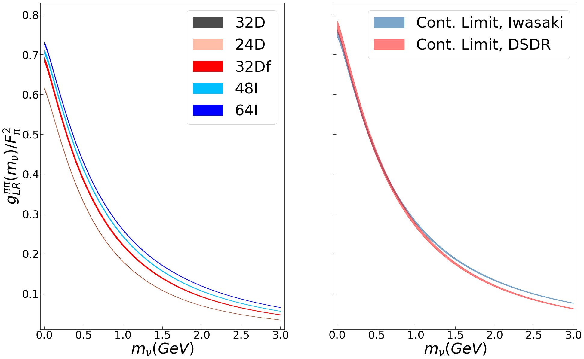
Figure 1: Lattice results of $g_{\text{LR}}^{\pi\pi}(m_{\nu})$ for each gauge ensemble (Left) and the continuum extrapolation based on Iwasaki and DSDR ensembles (Right). The 24D results are completely consistent with 32D results, making the latter nearly invisible in the figure.

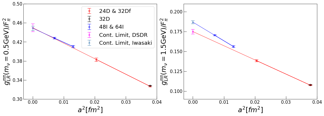
Figure 2: The continuum extrapolations with the linear fit ansatz of $a^{2}$ at some typical $m_{\nu}$ values. The left and right panels represent the case at $m_{\nu}=0.5$ GeV and $m_{\nu}=1.5$ GeV respectively.

We use the extrapolated result from Iwasaki ensembles as the final result and quote the deviation between Iwasaki and DSDR as the systematic uncertainty. The corresponding result of $g_{\text{LR}}^{\pi\pi}(m_{\nu})$ is given by the blue band in Fig. 3. The numerical values are listed in Appendix A. For comparison, we also show the results using the interpolation formula (green curve) and that using the RGE running (yellow band).

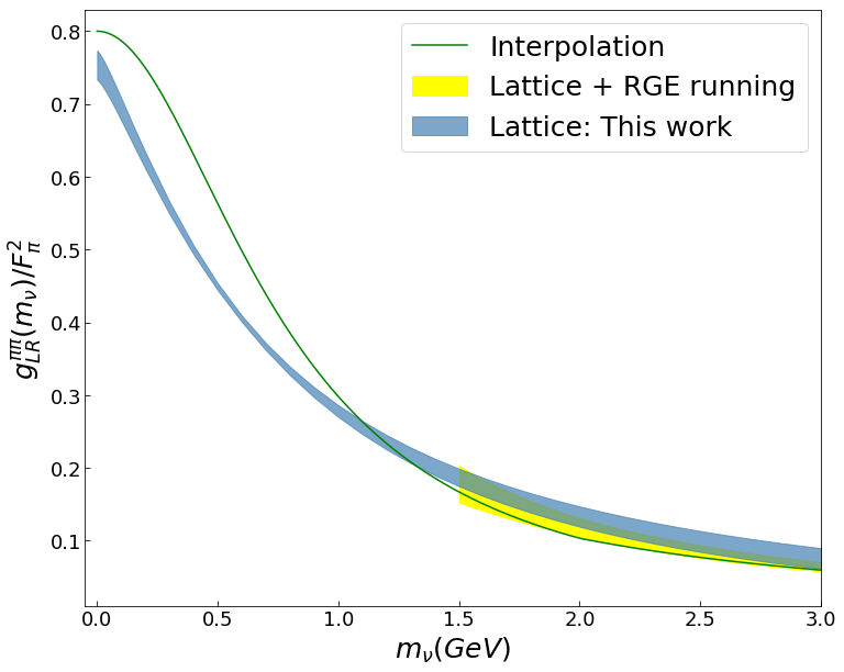
Figure 3: Comparison among the results of $g_{\text{LR}}^{\pi\pi}(m_{\nu})$ using lattice QCD (blue band), the interpolation formula (green curve) and the RGE running of $g_{4}^{\pi\pi}(\mu)$ (yellow band).

The idea on how to construct the interpolation formula is given in Ref. Dekens et al. (2020). To make Fig. 3 more comprehensive, we copy the expression of the interpolation formula here as

$$g_{\mathrm{LR}}^{\pi\pi}\left(m_{\nu}\right)=\frac{g_{\mathrm{LR}}^{\pi\pi}(0)}{1-m_{\nu}^{2}\frac{4g_{\mathrm{LR}}^{\pi\pi}(0)}{F_{\pi}^{2}}\left[\theta\left(m_{0}-m_{\nu}\right)g_{4}^{\pi\pi}\left(m_{0}\right)+\theta\left(m_{\nu}-m_{0}\right)g_{4}^{\pi\pi}\left(m_{\nu}\right)\right]^{-1}},$$ (22)

with $m_{0}=2$ GeV. The formula requires the inputs of $g_{\text{LR}}^{\pi\pi}(m_{\nu})$ at $m_{\nu}=0$ and $g_{4}^{\pi\pi}(m_{\nu})$ for $m_{\nu}\geq m_{0}$. For the former, it quotes the value from Eq. (4). For the latter, it uses the RGE running given in Eq. (7). Although the form seems simple, the interpolation formula captures the main $m_{\nu}$ dependence of $g_{\text{LR}}^{\pi\pi}(m_{\nu})$, which is reasonably consistent with the lattice results up to a 20% deviation at small $m_{\nu}$. Some reasons for the difference between the lattice results and the interpolating ones are explained as follows.

1. At $m_{\nu}=0$, the interpolation formula uses the input of pion mass splitting to determine $g_{\text{LR}}^{\pi\pi}(0)$. The electromagnetic corrections to pion mass only receive the contribution of the vector current insertions, while in the lattice QCD calculation both the vector and axial-vector parts are involved. Although in the leading order $\chi$PT, the contributions from vector and axial-vector part are equivalent, the lattice results indicate that the higher-order correction cannot be simply neglected.

2. When $m_{\nu}$ approaches zero, the interpolation formula suggests an $\mathcal{O}(m_{\nu}^{2})$ dependence of $g_{\text{LR}}^{\pi\pi}(m_{\nu})$, while the lattice results yield a non-zero derivative of $g_{\text{LR}}^{\pi\pi}(m_{\nu})$ with respect to $m_{\nu}$, see Fig. 4 for details. The reason for such behavior is explained in the Appendix B.

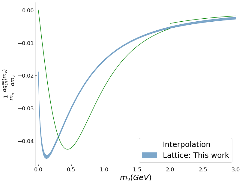
Figure 4: The derivative of $g_{\text{LR}}^{\pi\pi}(m_{\nu})$ with respect to $m_{\nu}$. At $m_{\nu}=0$, the interpolation formula yields $\frac{1}{m_{\pi}}\frac{\mathrm{d}g_{\text{LR}}^{\pi\pi}(m_{\nu})}{\mathrm{d}m_{\nu}}=0$ while the lattice result gives $\frac{1}{m_{\pi}}\frac{\mathrm{d}g_{\text{LR}}^{\pi\pi}(m_{\nu})}{\mathrm{d}m_{\nu}}=-\frac{1}{16\pi}$. This is one of the main differences between lattice and interpolating results.

At $m_{\nu}\gtrsim 1.5$ GeV, the lattice results of $g_{\text{LR}}^{\pi\pi}(m_{\nu})$ can be compared with the RGE running of $g_{4}^{\pi\pi}(\mu)$ by setting $\mu=m_{\nu}$ and assuming $g_{\text{LR}}^{\pi\pi}(m_{\nu})\simeq-\frac{F_{\pi}^{2}}{4m_{\nu}^{2}}g_{4}^{\pi\pi}(m_{\nu})$. As $g_{4,5}^{\pi\pi}(\mu)$ at $\mu=3$ GeV are determined using the lattice QCD input of pion local matrix element involving $O_{4}$ and $O_{5}$ Nicholson et al. (2018), this comparison can be considered as a consistency check between two independent lattice QCD calculations of the bilocal matrix elements and local matrix elements. A good consistency is found in the range of 1.5 GeV $\leq m_{\nu}\leq$ 3 GeV. We should remark that the agreement is partly due to the fact that at large $m_{\nu}$ the errors of the current lattice results are still quite large. The $O(\alpha_{s})$ effects neglected in the approximation of $g_{\text{LR}}^{\pi\pi}(m_{\nu})\simeq-\frac{F_{\pi}^{2}}{4m_{\nu}^{2}}g_{4}^{\pi\pi}(m_{\nu})$ may become important if the uncertainties are reduced.

We then evaluate how $g_{LR}^{\pi\pi}(m_{\nu})$ affects the decay amplitude $\mathcal{A}_{L}$ in Eq. (9). The decay amplitude is consisted of two parts, $\overline{\mathcal{M}}_{V}(m_{\nu})-\overline{\mathcal{M}}_{A}(m_{\nu})$ and $\overline{\mathcal{M}}_{V}(m_{\nu})+\overline{\mathcal{M}}_{A}(m_{\nu})$. Only the former piece receives the contributions from $g_{\text{LR}}^{\pi\pi}(m_{\nu})$. Using the lattice QCD results of $g_{\text{LR}}^{\pi\pi}(m_{\nu})$ and the available ¹³⁶Xe NMEs given in Ref.Dekens et al. (2020), we update the decay amplitude, namely $m_{\nu}(\overline{\mathcal{M}}_{V}(m_{\nu})-\overline{\mathcal{M}}_{A}(m_{\nu}))/(4m_{e})$, in Fig. 5. The peak location of the decay amplitude slightly shifts towards the larger value of $m_{\nu}$ when using the lattice inputs.

Here, the effects of $g_{\nu}^{NN}(m_{\nu})$ and $g_{LR}^{NN}(m_{\nu})$ are not included. They will also lead to a peak shape due to the suppression of decay amplitude at $m_{\nu}\to 0$ and $m_{\nu}\to\infty$ limits. To futher reduce the uncertainty of these LECs and determine the peak location, it is also necessary to calculate them from lattice QCD, which awaits future investigation.

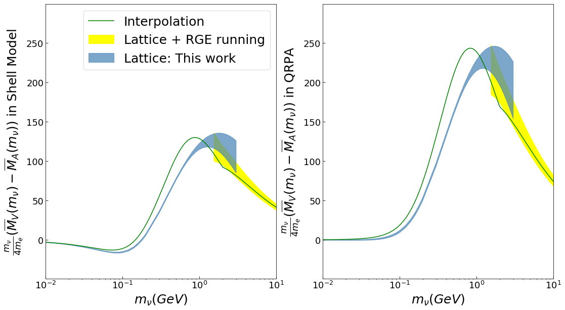
Figure 5: Comparison of the decay amplitude $m_{\nu}(\overline{\mathcal{M}}_{V}(m_{\nu})-\overline{\mathcal{M}}_{A}(m_{\nu}))/(4m_{e})$. Here, we take into account the impact of $g_{LR}^{\pi\pi}(m_{\nu})$ and neglect $g_{\nu}^{NN}(m_{\nu})$ and $g_{LR}^{NN}(m_{\nu})$. To determine the amplitude, we use ¹³⁶Xe NMEs in Ref. Dekens et al. (2020) which are evaluated using the Shell Model Menéndez (2018) (Left) and QRPA Jokiniemi et al. (2018) (Right). The inputs of the LECs $g_{\text{LR}}^{\pi\pi}(m_{\nu})$ are from lattice (blue band), interpolation formula (green curve) and RGE running (yellow band). The peak location of the decay amplitude shifts towards the larger value of $m_{\nu}$ when using the lattice inputs.

IV Conclusion

We perform a lattice QCD calculation of $g_{\text{LR}}^{\pi\pi}(m_{\nu})$ and its derivative in the range of 0 GeV$\leq m_{\nu}\leq 3$ GeV. Performing continuum extrapolation in the Iwasaki and DSDR ensembles separately, the lattice discretization effects are much suppressed. A good consistency with the previous lattice QCD calculation using local operators Nicholson et al. (2018) is found. Comparing our results with the naive interpolation formula at small $m_{\nu}$, we find a $\sim 20$ % deviation. The main reasons for the difference are two folds. First, the use of the pion mass splitting given in Eq. (4) provides a reasonably good but not sufficiently accurate value for $g_{\text{LR}}^{\pi\pi}(0)$. Second, we obtain the non-zero derivative of $g_{\text{LR}}^{\pi\pi}(m_{\nu})$ with respect to $m_{\nu}$ at $m_{\nu}=0$ while the interpolation formula yields zero. Using $g_{\text{LR}}^{\pi\pi}(m_{\nu})$ determined from lattice QCD, we present the neutrino mass dependence of single sterile neutrino contribution to $0\nu 2\beta$ decay amplitude. As pointed out by the Snowmass white paper Cirigliano et al. (2022), the EFTs that systematically describe $0\nu 2\beta$ decay amplitude in the few-nucleon and pion sector need to be complemented with values for LECs from lattice QCD. Our work serves as one more example for such purpose.

Appendix A Numerical values for $g_{LR}^{\pi\pi}(m_{\nu})$ on lattice

In Table 2 we list the lattice results of $g_{\text{LR}}^{\pi\pi}(m_{\nu})$, which can be used in the future phenomenological studies.

$m_{\nu}$ [GeV]	$g_{\text{LR}}^{\pi\pi}(m_{\nu})/F_{\pi}^{2}$	$m_{\nu}$ [GeV]	$g_{\text{LR}}^{\pi\pi}(m_{\nu})/F_{\pi}^{2}$	$m_{\nu}$ [GeV]	$g_{\text{LR}}^{\pi\pi}(m_{\nu})/F_{\pi}^{2}$	$m_{\nu}$ [GeV]	$g_{\text{LR}}^{\pi\pi}(m_{\nu})/F_{\pi}^{2}$
0	0.754(20)	0.2	0.622(11)	1.2	0.235(10)	2.2	0.118(14)
0.02	0.745(19)	0.3	0.557(8)	1.3	0.217(11)	2.3	0.111(14)
0.04	0.733(18)	0.4	0.499(6)	1.4	0.201(11)	2.4	0.105(14)
0.06	0.720(17)	0.5	0.449(5)	1.5	0.187(12)	2.5	0.099(14)
0.08	0.707(16)	0.6	0.405(4)	1.6	0.174(13)	2.6	0.094(14)
0.10	0.693(15)	0.7	0.366(5)	1.7	0.162(13)	2.7	0.089(14)
0.12	0.679(14)	0.8	0.333(6)	1.8	0.152(13)	2.8	0.084(14)
0.14	0.664(13)	0.9	0.304(7)	1.9	0.142(14)	2.9	0.080(14)
0.16	0.650(13)	1.0	0.278(8)	2.0	0.133(14)	3.0	0.076(14)
0.18	0.636(12)	1.1	0.255(9)	2.1	0.125(14)

Table 2: Lattice results of $g_{\text{LR}}^{\pi\pi}(m_{\nu})$ with $m_{\nu}$ from 0 GeV to 3 GeV.

Appendix B $g_{\text{LR}}^{\pi\pi}(m_{\nu})$ at small neutrino mass

As scalar propagator $S_{0}^{E}(x)$ contains a mass-square term, it seems that $g_{\text{LR}}^{\pi\pi}(m_{\nu})$ shall have a linear dependence on $m_{\nu}^{2}$ when $m_{\nu}\to 0$. However, we will demonstrate here that this is not the case. We write down the pion intermediate-state contribution to the hadronic function $H_{VV}^{E}(x)$ as

$$H_{\pi}(x)=-\int\frac{d^{3}p}{(2\pi)^{3}2E_{\pi,p}}m_{\pi}(m_{\pi}+E_{\pi,p})[F^{(\pi)}(q^{2})]^{2}e^{-(E_{\pi,p}-m_{\pi})|t|}e^{i\vec{p}\cdot\vec{x}}$$ (23)

where $F^{(\pi)}(q^{2})$ is pion electromagnetic form factor introduced by using the isospin rotation. $q^{2}=2m_{\pi}(m_{\pi}-E_{\pi,p})$ comes from the momentum transfer between the charged pion in the initial state and the neutral pion in the intermediate state. The contribution of $H_{\pi}(x)$ propagates into $g_{\text{LR}}^{\pi\pi}(m_{\nu})$ and yields

$$g_{\text{LR},\pi}^{\pi\pi}(m_{\nu})=\frac{1}{8}\int\frac{d^{3}p}{(2\pi)^{3}}\frac{m_{\pi}(m_{\pi}+E_{\pi,p})[F^{(\pi)}(q^{2})]^{2}}{E_{\pi,p}E_{\nu,p}(E_{\pi,p}-m_{\pi}+E_{\nu,p})},$$ (24)

where we define $E_{\pi,p}^{2}=p^{2}+m_{\pi}^{2}$ and $E_{\nu,p}^{2}=p^{2}+m_{\nu}^{2}$.

At small $m_{\nu}$, we can take a scale $\Lambda$ satisfying $m_{\nu}\ll\Lambda\ll m_{\pi}$. In the momentum region $p<\Lambda$, the integral can be simplified as

$$g_{\text{LR},\pi}^{\pi\pi}(m_{\nu})|_{p<\Lambda}=\frac{m_{\pi}}{8\pi^{2}}\int_{0}^{\Lambda}\mathrm{d}p\,\frac{p^{2}}{p^{2}+m_{\nu}^{2}}\left(1+\mathcal{O}\left(\frac{p^{2}}{m_{\pi}^{2}}\right)\right).$$ (25)

We then consider the derivative of

$$\frac{\mathrm{d}g_{\text{LR},\pi}^{\pi\pi}(m_{\nu})|_{p<\Lambda}}{\mathrm{d}m_{\nu}} =-\frac{m_{\pi}m_{\nu}}{4\pi^{2}}\int_{0}^{\Lambda}\mathrm{d}p\,\frac{p^{2}}{(p^{2}+m_{\nu}^{2})^{2}}\left(1+\mathcal{O}\left(\frac{p^{2}}{m_{\pi}^{2}}\right)\right)$$ (26)

$$=-\frac{m_{\pi}m_{\nu}}{4\pi^{2}}\left(\frac{\pi}{4m_{\nu}}-\frac{1}{2\Lambda}+\cdots\right).$$

In the momentum region of $p\geq\Lambda$, one can simply take a Taylor expansion of $1/(p^{2}+m_{\nu}^{2})=1/p^{2}-m_{\nu}^{2}/p^{4}+\cdots$. The derivative yields zero at $m_{\nu}=0$. Thus, we can conclude that

$$\frac{\mathrm{d}g_{\text{LR},\pi}^{\pi\pi}(m_{\nu})}{\mathrm{d}m_{\nu}}\Big{|}_{m_{\nu}=0}=-\frac{m_{\pi}}{16\pi}.$$ (27)

For the contributions from the excited states, as the integral only contains a factor of $1/\sqrt{p^{2}+m_{\nu}^{2}}$ rather than $1/(p^{2}+m_{\nu}^{2})$ at small $m_{\nu}$, one can show that the derivative vanish when $m_{\nu}\to 0$. This means that $\frac{\mathrm{d}g_{LR}^{\pi\pi}(m_{\nu})}{\mathrm{d}m_{\nu}}\big{|}_{m_{\nu}=0}$ is a structure-independent value. In Fig. 4, we obtain the lattice result of $\frac{1}{m_{\pi}}\frac{\mathrm{d}g_{LR}^{\pi\pi}(m_{\nu})}{\mathrm{d}m_{\nu}}\big{|}_{m_{\nu}=0}=-0.0201(16)$, which is well consistent with the expectation of $-1/(16\pi)\approx-0.0199$.

References

- Dekens et al. (2020) W. Dekens, J. de Vries, K. Fuyuto, E. Mereghetti, and G. Zhou, JHEP 06, 097 (2020), arXiv:2002.07182 [hep-ph] .
- Nicholson et al. (2018) A. Nicholson et al., Phys. Rev. Lett. 121, 172501 (2018), arXiv:1805.02634 [nucl-th] .
- Agostini et al. (2019) M. Agostini et al. (GERDA), Science 365, 1445 (2019), arXiv:1909.02726 [hep-ex] .
- Gando et al. (2016) A. Gando et al. (KamLAND-Zen), Phys. Rev. Lett. 117, 082503 (2016), [Addendum: Phys. Rev. Lett.117,no.10,109903(2016)], arXiv:1605.02889 [hep-ex] .
- Alduino et al. (2018) C. Alduino et al. (CUORE), Phys. Rev. Lett. 120, 132501 (2018), arXiv:1710.07988 [nucl-ex] .
- Albert et al. (2018) J. B. Albert et al. (EXO), Phys. Rev. Lett. 120, 072701 (2018), arXiv:1707.08707 [hep-ex] .
- Azzolini et al. (2018) O. Azzolini et al. (CUPID-0), Phys. Rev. Lett. 120, 232502 (2018), arXiv:1802.07791 [nucl-ex] .
- Alvis et al. (2019) S. I. Alvis et al. (Majorana), Phys. Rev. C100, 025501 (2019), arXiv:1902.02299 [nucl-ex] .
- Agostini et al. (2020) M. Agostini et al. (GERDA), Phys. Rev. Lett. 125, 252502 (2020), arXiv:2009.06079 [nucl-ex] .
- Armengaud et al. (2021) E. Armengaud et al. (CUPID), Phys. Rev. Lett. 126, 181802 (2021), arXiv:2011.13243 [nucl-ex] .
- Adams et al. (2022) D. Q. Adams et al. (CUORE), Nature 604, 53 (2022), arXiv:2104.06906 [nucl-ex] .
- Abe et al. (2022) S. Abe et al. (KamLAND-Zen), (2022), arXiv:2203.02139 [hep-ex] .
- Cirigliano et al. (2022) V. Cirigliano et al., (2022), arXiv:2203.12169 [hep-ph] .
- Cirigliano et al. (2017a) V. Cirigliano, W. Dekens, M. Graesser, and E. Mereghetti, Phys. Lett. B 769, 460 (2017a), arXiv:1701.01443 [hep-ph] .
- Cirigliano et al. (2017b) V. Cirigliano, W. Dekens, J. de Vries, M. L. Graesser, and E. Mereghetti, JHEP 12, 082 (2017b), arXiv:1708.09390 [hep-ph] .
- Cirigliano et al. (2018a) V. Cirigliano, W. Dekens, E. Mereghetti, and A. Walker-Loud, Phys. Rev. C 97, 065501 (2018a), [Erratum: Phys.Rev.C 100, 019903 (2019)], arXiv:1710.01729 [hep-ph] .
- Pastore et al. (2018) S. Pastore, J. Carlson, V. Cirigliano, W. Dekens, E. Mereghetti, and R. B. Wiringa, Phys. Rev. C 97, 014606 (2018), arXiv:1710.05026 [nucl-th] .
- Cirigliano et al. (2018b) V. Cirigliano, W. Dekens, J. De Vries, M. L. Graesser, E. Mereghetti, S. Pastore, and U. Van Kolck, Phys. Rev. Lett. 120, 202001 (2018b), arXiv:1802.10097 [hep-ph] .
- Cirigliano et al. (2018c) V. Cirigliano, W. Dekens, J. de Vries, M. L. Graesser, and E. Mereghetti, JHEP 12, 097 (2018c), arXiv:1806.02780 [hep-ph] .
- Cirigliano et al. (2019) V. Cirigliano, W. Dekens, J. De Vries, M. L. Graesser, E. Mereghetti, S. Pastore, M. Piarulli, U. Van Kolck, and R. B. Wiringa, Phys. Rev. C 100, 055504 (2019), arXiv:1907.11254 [nucl-th] .
- Cirigliano et al. (2021a) V. Cirigliano, W. Dekens, J. de Vries, M. Hoferichter, and E. Mereghetti, Phys. Rev. Lett. 126, 172002 (2021a), arXiv:2012.11602 [nucl-th] .
- Cirigliano et al. (2021b) V. Cirigliano, W. Dekens, J. de Vries, M. Hoferichter, and E. Mereghetti, JHEP 05, 289 (2021b), arXiv:2102.03371 [nucl-th] .
- Cirigliano et al. (2020) V. Cirigliano, W. Detmold, A. Nicholson, and P. Shanahan, (2020), 10.1016/j.ppnp.2020.103771, arXiv:2003.08493 [nucl-th] .
- Shanahan et al. (2017) P. E. Shanahan, B. C. Tiburzi, M. L. Wagman, F. Winter, E. Chang, Z. Davoudi, W. Detmold, K. Orginos, and M. J. Savage, Phys. Rev. Lett. 119, 062003 (2017), arXiv:1701.03456 [hep-lat] .
- Tiburzi et al. (2017) B. C. Tiburzi, M. L. Wagman, F. Winter, E. Chang, Z. Davoudi, W. Detmold, K. Orginos, M. J. Savage, and P. E. Shanahan, Phys. Rev. D 96, 054505 (2017), arXiv:1702.02929 [hep-lat] .
- Feng et al. (2019) X. Feng, L.-C. Jin, X.-Y. Tuo, and S.-C. Xia, Phys. Rev. Lett. 122, 022001 (2019), arXiv:1809.10511 [hep-lat] .
- Tuo et al. (2019) X.-Y. Tuo, X. Feng, and L.-C. Jin, Phys. Rev. D 100, 094511 (2019), arXiv:1909.13525 [hep-lat] .
- Detmold and Murphy (2020) W. Detmold and D. J. Murphy (NPLQCD), (2020), arXiv:2004.07404 [hep-lat] .
- Feng et al. (2021) X. Feng, L.-C. Jin, Z.-Y. Wang, and Z. Zhang, Phys. Rev. D 103, 034508 (2021), arXiv:2005.01956 [hep-lat] .
- Davoudi and Kadam (2020) Z. Davoudi and S. V. Kadam, Phys. Rev. D 102, 114521 (2020), arXiv:2007.15542 [hep-lat] .
- Davoudi and Kadam (2021) Z. Davoudi and S. V. Kadam, Phys. Rev. Lett. 126, 152003 (2021), arXiv:2012.02083 [hep-lat] .
- Davoudi and Kadam (2022) Z. Davoudi and S. V. Kadam, Phys. Rev. D 105, 094502 (2022), arXiv:2111.11599 [hep-lat] .
- Akhmedov et al. (1998) E. K. Akhmedov, V. A. Rubakov, and A. Y. Smirnov, Phys. Rev. Lett. 81, 1359 (1998), arXiv:hep-ph/9803255 .
- Asaka et al. (2005) T. Asaka, S. Blanchet, and M. Shaposhnikov, Phys. Lett. B 631, 151 (2005), arXiv:hep-ph/0503065 .
- Asaka and Shaposhnikov (2005) T. Asaka and M. Shaposhnikov, Phys. Lett. B 620, 17 (2005), arXiv:hep-ph/0505013 .
- Shaposhnikov (2007) M. Shaposhnikov, Nucl. Phys. B 763, 49 (2007), arXiv:hep-ph/0605047 .
- Canetti et al. (2013) L. Canetti, M. Drewes, and M. Shaposhnikov, Phys. Rev. Lett. 110, 061801 (2013), arXiv:1204.3902 [hep-ph] .
- Hernández et al. (2016) P. Hernández, M. Kekic, J. López-Pavón, J. Racker, and J. Salvado, JHEP 08, 157 (2016), arXiv:1606.06719 [hep-ph] .
- Ghiglieri and Laine (2017) J. Ghiglieri and M. Laine, JHEP 05, 132 (2017), arXiv:1703.06087 [hep-ph] .
- del Aguila et al. (2009) F. del Aguila, S. Bar-Shalom, A. Soni, and J. Wudka, Phys. Lett. B 670, 399 (2009), arXiv:0806.0876 [hep-ph] .
- Cirigliano et al. (2013) V. Cirigliano, M. Gonzalez-Alonso, and M. L. Graesser, JHEP 02, 046 (2013), arXiv:1210.4553 [hep-ph] .
- Asaka et al. (2016) T. Asaka, S. Eijima, and H. Ishida, Phys. Lett. B 762, 371 (2016), arXiv:1606.06686 [hep-ph] .
- Liao and Ma (2017) Y. Liao and X.-D. Ma, Phys. Rev. D 96, 015012 (2017), arXiv:1612.04527 [hep-ph] .
- Liao and Ma (2019) Y. Liao and X.-D. Ma, JHEP 03, 179 (2019), arXiv:1901.10302 [hep-ph] .
- Liao et al. (2020) Y. Liao, X.-D. Ma, and Q.-Y. Wang, JHEP 08, 162 (2020), arXiv:2005.08013 [hep-ph] .
- Liao and Ma (2020) Y. Liao and X.-D. Ma, JHEP 11, 152 (2020), arXiv:2007.08125 [hep-ph] .
- Jokiniemi et al. (2018) L. Jokiniemi, H. Ejiri, D. Frekers, and J. Suhonen, Phys. Rev. C 98, 024608 (2018).
- Menéndez (2018) J. Menéndez, J. Phys. G 45, 014003 (2018), arXiv:1804.02105 [nucl-th] .
- Christ et al. (2016) N. H. Christ, X. Feng, A. Portelli, and C. T. Sachrajda (RBC, UKQCD), Phys. Rev. D 93, 114517 (2016), arXiv:1605.04442 [hep-lat] .
- Bai et al. (2017) Z. Bai, N. H. Christ, X. Feng, A. Lawson, A. Portelli, and C. T. Sachrajda, Phys. Rev. Lett. 118, 252001 (2017), arXiv:1701.02858 [hep-lat] .
- Feng and Jin (2019) X. Feng and L. Jin, Phys. Rev. D 100, 094509 (2019), arXiv:1812.09817 [hep-lat] .
- Feng et al. (2022) X. Feng, L. Jin, and M. J. Riberdy, Phys. Rev. Lett. 128, 052003 (2022), arXiv:2108.05311 [hep-lat] .
- Christ et al. (2020) N. H. Christ, X. Feng, J. Lu-Chang, and C. T. Sachrajda, PoS LATTICE2019, 259 (2020).
- Christ et al. (2021) N. H. Christ, X. Feng, L.-C. Jin, and C. T. Sachrajda, Phys. Rev. D 103, 014507 (2021), arXiv:2009.08287 [hep-lat] .
- Tuo et al. (2022) X.-Y. Tuo, X. Feng, L.-C. Jin, and T. Wang, Phys. Rev. D 105, 054518 (2022), arXiv:2103.11331 [hep-lat] .
- Meng et al. (2021) Y. Meng, X. Feng, C. Liu, T. Wang, and Z. Zou, (2021), arXiv:2109.09381 [hep-lat] .
- Fu et al. (2022) Y. Fu, X. Feng, L.-C. Jin, and C.-F. Lu, Phys. Rev. Lett. 128, 172002 (2022), arXiv:2202.01472 [hep-lat] .
- Blum et al. (2016a) T. Blum et al. (RBC, UKQCD), Phys. Rev. D 93, 074505 (2016a), arXiv:1411.7017 [hep-lat] .
- Blum et al. (2016b) T. Blum et al. (RBC, UKQCD), Phys. Rev. D 93, 074505 (2016b), arXiv:1411.7017 [hep-lat] .