Stochastic Deep-Ritz for Parametric Uncertainty Quantification

Abstract

Scientific machine learning has become an increasingly important tool in materials science and engineering. It is particularly well suited to tackle material problems involving many variables or to allow rapid construction of surrogates of material models, to name just a few. Mathematically, many problems in materials science and engineering can be cast as variational problems. However, handling of uncertainty, ever present in materials, in the context of variational formulations remains challenging for scientific machine learning. In this article, we propose a deep-learning-based numerical method for solving variational problems under uncertainty. Our approach seamlessly combines deep-learning approximation with Monte-Carlo sampling. The resulting numerical method is powerful yet remarkably simple. We assess its performance and accuracy on a number of variational problems.

1 Introduction

Randomness and uncertainty are ubiquitous in materials science and engineering. In order to facilitate analysis, and ultimately design, of materials, it is essential to accurately quantify the uncertainty in material models. A good case in point is additive manufacturing of materials. Additive manufacturing commonly involves numerous sources of uncertainty such as laser power, material composition or particle size. The uncertainty ultimately influences the material microstructure and hence, in turn, affects the mechanical performance of manufactured parts. Therefore, it is critical to take the uncertainty into account as to clear the way for robust additive manufacturing. From the mathematical modeling perspective, the uncertainty is frequently modeled as the random input data in the form of a random field $\kappa$ to a (stochastic) variational problem

$$\min_{u}\mathbb{E}\left[\int_{D}I(x,u,\nabla u;\kappa)\,dx\right]$$ (1)

for a Lagrangian $I$ depending on the random field $\kappa$.

Traditionally, solutions of (1) are sought by first computing the associated strong form and then solving the resulting differential equation by numerical methods for stochastic differential equations. A great number of computational methodologies have been developed to solve stochastic differential equations. Among them, stochastic collocation (SC), stochastic Galerkin (SG), and Monte Carlo (MC)/quasi Monte Carlo (QMC) are the three mainstream approaches. SC aims to first solve the deterministic counterpart of a stochastic differential equation on a set of collocation points and then interpolate over the entire image space of the random element [1, 2, 3]. Hence, the method is non-intrusive, meaning that it can take advantage of existing solvers developed for deterministic problems. Similarly, MC is non-intrusive since it relies on taking sample average over a set of deterministic solutions computed from a set of realizations of the random field [4, 5, 6]. In contrast, SG is considered as intrusive since it requires a construction of discretization of both the stochastic space and physical space simultaneously and, as a result, it commonly tends to produce large systems of algebraic equations whose solutions are needed [4, 7, 8, 9, 10]. However, these algebraic systems differ appreciably from their deterministic counterparts and thus existing deterministic solvers can rarely be utilized.

It is important to stress that all traditional numerical methods for stochastic differential equations suffer from the curse of dimensionality and hence tend to be limited to low dimensional problems (e.g., $D\subset\mathbb{R}^{2}$ or $D\subset\mathbb{R}^{3}$). Recently, deep neural networks (DNN) have garnered some acceptance in computational science and engineering, and deep-learning-based computational methods have been universally recognized as potentially capable of overcoming the curse of dimensionality [11, 12]. Depending on how the loss function is formulated, deep-learning-based methods for deterministic differential equations can broadly be classified into three categories: 1) residual based minimization, 2) deep backward stochastic differential equations (BSDE) and 3) energy based minimization. Both the physics informed neural networks (PINNs) [13, 14] and the deep Galerkin methods (DGMs) [15] belong to the category of residual minimization. PINNs aim to minimize the total residual loss based on a set of discrete data points in the domain $D$. Similarly, DGMs rely on minimizing the loss function induced by the $L^{2}$ error. We also refer [16, 17] for a similar approach. In contrast, the deep-BSDE methods exploit the intrinsic connection between PDEs and BSDEs in the form of the nonlinear Feynman-Kac formula to recast a PDE as a stochastic control problem that is solved by reinforcement learning techniques [18, 19, 20, 21, 22]. See [23] for a recent work on interpolating between PINNs and deep BSDEs. Finally, energy methods construct the loss function by taking advantage of the variational formulation of elliptic PDEs [24, 25, 26, 27]. As a comparable approach, in [28] the Dynkin formula for overdamped Langevin dynamics is employed to construct a weighted variational loss function. We refer an interested reader to [29, 30, 31] for an in-depth overview of deep-learning-based methods for solving PDEs.

Lately, extensions of the deep-learning approaches for PDEs with random coefficients have been proposed. For example, convolutional neural networks mimicking image-to-image regression in computer vision have been employed to learn the input-to-output mapping for parametric PDEs [26, 32, 33]. However, these methods, by design, are mesh-dependent and therefore aim to discover a mapping between finite dimensional spaces. In contrast, operator learning methods, such as the deep operator network (ONET) [34] and the Fourier neural operator (FNO) [35], aim at learning a mesh-free, infinite dimensional operator with specialized network architectures. Let us also point out that all these methods tend to identify a mapping $u:\kappa\to u(\kappa)$, i.e., from the random field to the solution. In practice, the sampling of $\kappa$ is often reliant on the Karhunen–Loève expansion to parameterize $\kappa$ by means of a finite dimensional random vector $Z$. Taking this fact into account, in this article we propose to directly learn a mapping $u:(x,Z)\to u(x,Z)$, i.e., from the joint space of $x$ and $Z$ to the solution. We empirically show that our approach achieves comparable accuracy with traditional methods even with a generic fully connected neural network architecture. More importantly, however, ONET and FNO are supervised by design and rely on the mean square loss function to facilitate training. Such a loss function rarely takes the underlying physics into account in a direct manner and customarily depends on sampling of the solution throughout the domain. In order to sidestep the above difficulties, we instead employ (1) directly. We emphasize that our approach possesses a fundamental advantage over the approaches reliant on stochastic differential equations. Namely, after approximating the solution $u$ by a DNN, the functional provides a natural loss function. Hence, the physical laws encoded in (1) are seamlessly incorporated when a minimizer is computed. Our method can be considered as an extension of the deep-Ritz method in [24] to the stochastic setting and henceforth we refer to it as the stochastic deep-Ritz method.

The remainder of the article is organized as follows. Section 2 describes the general framework for solving the stochastic variational problem by means of DNN. In Section 3, we propose the DNN based approach and present the stochastic deep-Ritz method. Finally, numerical benchmarks are presented in Section 4.

2 The stochastic variational problem

Let $D\subset\mathbb{R}^{d}$ be a bounded open set with a Lipschitz boundary $\partial D$ and $(\Omega,\mathcal{F},\mathbb{P})$ be a probability space, where $\Omega$ is the sample space, $\mathcal{F}\subset 2^{\Omega}$ is a $\sigma$-algebra of all possible events and $\mathbb{P}:\mathcal{F}\to[0,1]$ is a probability measure. We consider functionals of the type

$$J(u)=\mathbb{E}\left[\int_{D}I(x,u,\nabla u;\kappa(x,\omega))\,dx\right]$$ (2)

where $I:\mathbb{R}^{d}\times\mathbb{R}^{N}\times\mathbb{R}^{d\times N}\to\mathbb{R}$ is the Lagrangian, $u:\bar{D}\times\Omega\to\mathbb{R}^{N}$ is the solution of interest, and $\kappa:\bar{D}\times\Omega\to\mathbb{R}$ is the random input field. Here $\bar{D}=D\cup\partial D$ denotes the closure of $D$ in $\mathbb{R}^{d}$ and $\nabla$ is the gradient with respect to the spatial coordinate $x$. We suppose that the Lagrangian $I$ is of class $C^{1}$ on an open subset of $\mathbb{R}^{d}\times\mathbb{R}^{N}\times\mathbb{R}^{d\times N}$. Moreover, we make the usual assumption that the random fields $\kappa$ is parameterized by a finite dimensional random vector $Z=(Z_{1},\ldots,Z_{K}):\Omega\to\Gamma\subset\mathbb{R}^{K}$, i.e., there exists finitely many uncorrelated random variables $Z_{1},\ldots,Z_{K}$ such that the random field is of the form

$$\kappa(x,\omega)=\kappa(x,Z(\omega))$$

and hence (2) reduces to

$$J(u)=\mathbb{E}_{Z}\left[\int_{D}I(x,u,\nabla u;\kappa(x,Z))\,dx\right],$$ (3)

where the expectation is taken with respect to the random vector $Z$. We are interested in solving the following stochastic variation problems

$$\min_{u\in\mathcal{U}}J(u)$$ (4)

over a suitable functional space $\mathcal{U}$. There exists a substantial body of literature dedicated to studying the existence of solutions of (4) (see, for example, [36, 37]). We direct the reader to Theorem 1 in the appendix where we derive the conditions for existence of such solutions for a quadratic Lagrangian.

Numerical solutions of (4) are notoriously difficult to obtain. While many techniques have been proposed, they primarily rely on, first, reducing the minimization problem (4) to a random input PDE and, second, numerically solving the resulting random input PDE by classical techniques such as stochastic collocation (SC) [1, 2, 3], stochastic Galerkin (SG) [7, 4, 8, 9, 10] and Monte Carlo (MC) [4, 5, 6]. In contrast to these techniques, we proposed in [38] an approach to seek solutions of (4) directly by a combination of polynomial chaos expansion (PCE) and stochastic gradient descent (SGD). However, the approach relies on the approximation over the tensor product space of $D$ and $\Omega$. In what follows, we introduce a DNN-based method which does not require such approximation over the tensor product space.

3 Stochastic deep-Ritz: deep learning based UQ

3.1 Preliminaries on neural networks

Let us now briefly review some preliminaries on DNN and set up the finite dimensional functional space induced by DNN. A standard fully-connected DNN of depth $L>2$ with input dimension $N_{0}$ and output dimension $N_{L}$ is determined by a tuple

$$\Phi=\{(T_{1},\sigma_{1}),\ldots,(T_{L},\sigma_{L})\},$$

where $T_{l}(x)=W_{l}x+b_{l}$ is an affine transformation with weight matrix $W_{l}\in\mathbb{R}^{N_{l-1}\times N_{l}}$ and bias vector $b_{l}\in\mathbb{R}^{N_{l}}$ and $\sigma_{l}:\mathbb{R}^{N_{l}}\to\mathbb{R}^{N_{l}}$ is a nonlinear activation function. We say the DNN $\Phi$ is of width $W$ if $W=\max_{l=1,\ldots,L}N_{l}$. We denote

$$\theta=(W_{1},b_{1},\ldots,W_{L},b_{L})$$

the weight parameters of $\Phi$ and

$$\sigma=(\sigma_{1},\ldots,\sigma_{L})$$

the set of activation functions of $\Phi$. For a fixed set of activation functions $\sigma$, the DNN $\Phi$ is completely determined by the weight parameters $\theta$ and hence in the sequel we write $\Phi=\Phi_{\theta}$ to emphasize the dependence on $\theta$. Each DNN $\Phi_{\theta}$ induces a function

$$u_{\theta}=R(\Phi_{\theta}):\mathbb{R}^{N_{0}}\to\mathbb{R}^{N_{L}},\quad x\mapsto\sigma_{L}\circ T_{L}\circ\ldots\circ\sigma_{1}\circ T_{1}.$$

We refer to $R(\Phi_{\theta})$ as the realization of the DNN $\Phi_{\theta}$. The set of all DNNs of depth $L$ and width $W$, denoted by $\mathcal{N}_{L,W}$, induces a functional space $\mathcal{U}_{L,W}$ consisting of all realizations of DNNs contained in $\mathcal{N}_{L,W}$, i.e.,

$$\mathcal{U}_{L,W}=\left\{u_{\theta}:\mathbb{R}^{N_{0}}\to\mathbb{R}^{N_{L}}~{}|~{}u_{\theta}=R(\Phi_{\theta}),\Phi_{\theta}\in\mathcal{N}_{L,W}\right\}.$$

Approximating a function $u$ by DNNs in $\mathcal{N}_{L,W}$ amounts to selecting a realization $u_{\theta}\in\mathcal{U}_{L,W}$ minimizing an appropriate loss functions. Therefore, a DNN along with its realization provide together a surrogate over the functional space $\mathcal{U}_{L,W}$.

3.2 The stochastic deep-Ritz method

We are now in a position to discuss solving the stochastic variational problem (4) with DNN. To avoid the deterministic approximation of the integration over the physical domain $D$, we introduce a $d$-dimensional random vector $X$ with the uniform density function $\mu(x)$ supported on $D$ and rewrite (4) into the following fully probabilistic form:

$$\min_{u\in\mathcal{U}}J(u)\quad\textrm{with}\quad J(u)=\mathbb{E}\left[I(X,u(X,Z),\nabla u(X,Z);\kappa(X,Z))\right],$$ (5)

where the expectation $\mathbb{E}$ is now taken with respect to both $X$ and $Z$ and we implicitly assume that the volume of $D$ with respect to $\mu$ is normalized to $1$, i.e., $\int_{D}\mu(x)\,dx=1$.

Next, we seek an approximate solution of the problem (5) in the neural network space $\mathcal{U}_{L,W}$. The functional in (5) provides a natural loss function that can be optimized with DNN using SGD methods. Specifically, we consider a class of DNNs $\Phi_{\theta}$ (parameterized by $\theta$) with input dimension $d+K$ and output dimension $1$ whose realizations approximate the true solution $u(x,z)$, i.e.,

$$u(x,z)\approx u_{\theta}(x,z)=R(\Phi_{\theta})(x,z),$$

through minimizing the functional (5). This leads to the following finite dimensional optimization problem:

$$\min_{u_{\theta}\in\mathcal{U}_{L,W}}J(u_{\theta})\quad\textrm{with}\quad J(u_{\theta})=\mathbb{E}\left[I(X,u_{\theta}(X,Z),\nabla u_{\theta}(X,Z);\kappa(X,Z))\right],$$

where the optimization is over the space $\mathcal{U}_{L,W}$, i.e., the function space induced by the realizations of DNNs with depth $L$ and width $W$. The fully-connected DNN architecture that we employ in this work is schematically represented in Figure 1. Although there exist more sophisticated NN architectures, e.g., residual NN [39] and Unet [40], we demonstrate in Section 4 that a rather simple fully-connected DNN is capable of learning the solution with high accuracy.

Unlike the finite element method, which takes the boundary conditions into account by design, hard-constraint boundary conditions for DNN-based methods can only be enforced for simple geometry of $D$ [41, 42, 43]. Therefore, we enforce the soft-constraint boundary condition by introducing a penalty term to compensate for the boundary condition and obtain the final loss function:

$$\min_{u_{\theta}\in\mathcal{U}_{L,W}}J(u_{\theta})$$ (6)

with

$$J(u_{\theta})=\mathbb{E}\left[I(X,u_{\theta}(X,Z),\nabla u_{\theta}(X,Z);\kappa(X,Z))\right]+\beta\mathbb{E}\left[|u_{\theta}(S,Z)|^{2}\right],$$

where $\beta$ is the penalty coefficient and $S$ is a random vector with a uniform distribution over the boundary $\partial D$. Here, the first and second expectations are taken with respect to $(X,Z)$ and $(S,Z)$, respectively. We use the same $\mathbb{E}$ to denote the two expectations for notational simplicity. It should be emphasized that, other than the DNN approximation error, the penalty term often introduces an additional source of errors into the problem and hence changes the ground truth solution. However, we expect that the soft constraint error is negligible compared to the DNN approximation error for large penalty $\beta$. The stochastic optimization problem (6) can be naturally solved by the SGD algorithm or its variants and the final stochastic deep-Ritz algorithm is presented in Algorithm 1.

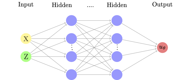
Figure 1: The fully-connected neural network architecture employed in the stochastic deep-Ritz solver.

Algorithm 1 The stochastic deep-Ritz algorithm

Input: A fully-connected DNN $\Phi_{\theta}$; number of training iterations $N_{e}$; mini-batch size $M$; penalty coefficient $\beta$; learning rate $\eta_{n}$;
Output: A DNN surrogate $\Phi_{\theta}$ with realization $u_{\theta}$.

1:for $n=1:N_{e}$ do

2:     Generate a minibatch of samples $(X_{m},S_{m},Z_{m})$ for $m=1,\ldots,M$,

3:     Evaluate the NN realizations $u_{\theta}(X_{m},Z_{m})$ and $u_{\theta}(S_{m},Z_{m})$,

4:     Compute the stochastic gradient estimator $g(\theta_{n};X_{m},S_{m},Z_{m})$ such that

$$\mathbb{E}\left[g(\theta_{n};X_{m},S_{m},Z_{m})\right]=\nabla_{\theta}J(\theta_{n}),\quad m=1,\ldots,M,$$

5:     Compute the mini-batch average:

$$\bar{g}(\theta_{n})=\frac{1}{M}\sum_{m=1}^{M}g(\theta_{n};X_{m},S_{m},Z_{m}),$$

6:     Update the DNN parameters: $\theta_{n}\leftarrow\theta_{n}-\eta_{n}\bar{g}(\theta_{n})$.

Remark 3.1.

Some remarks on Algorithm 1 are in order.

1. A natural choice for the stochastic gradient estimator is

   $$g(\theta;X,S,Z)=\nabla_{\theta}\left\{I(X,u_{\theta}(X,Z),\nabla u_{\theta}(X,Z);\kappa(X,Z))+\beta\left|u_{\theta}(S,Z)\right|^{2}\right\},$$

   which can be easily obtained by automatic differentiation in any deep learning frameworks. However, it is possible to construct more efficient estimators through variance reduction techniques [44, 45]. This will be the focus of another work.

2. The numerical consistency of the stochastic deep-Ritz method, i.e., the minimizer of $J(u_{\theta})$ over $\mathcal{U}_{L,W}$ converges (weakly) to the minimizer of $J(u)$ over $\mathcal{U}$, relies on justifying the $\Gamma$-convergence when either the depth $L\to\infty$ or the width $W\to\infty$ (see e.g.,  [46]). We refer interested reader to [27] for a proof in the deterministic setting.

3. In practice, more efficient SGD variants such as Adam can be used to expedite the training of NNs [47].

It should be emphasized that the stochastic deep-Ritz method learns a deterministic function $u_{\theta}$ mapping the random variables $X$ and $Z$ to the random variable $u_{\theta}(X,Z)$. Similar applications of DNNs are common in deep learning. For instance, the generator of a GAN learns a mapping from Gaussian samples to samples from the desired distribution. Similarly, the DNN in our method takes samples from $(X,Z)$ and learns how to generate samples from $u_{\theta}(X,Z)$, that is, the DNN learns the transformation between the input $(X,Z)$ and solution $u_{\theta}(X,Z)$. In comparison with the traditional approaches, e.g., SC and PC, which obtain an explicit approximation to the solution, the proposed methodology should be considered as an implicit method since it only allows us to learn an approximated simulator of the true solution $u(X,Z)$. However, note that for stochastic problems one is often not interested in the analytical solutions but rather the statistical properties (e.g., moments, distribution) of the solution. In practice, all statistical properties of the solution can be easily computed through sampling directly from the learned neural DNN.

4 Numerical experiments

In order to demonstrate the efficacy and accuracy of the proposed method, we assess its numerical performance by testing it on a class of stochastic variational problems with quadratic Lagrangian, i.e.,

$$\min_{u\in\mathcal{U}}J(u)\quad\textrm{with}\quad J(u)=\mathbb{E}\left[\int_{D}\frac{1}{2}\kappa(x,Z)|\nabla u(x,Z)|^{2}-f(x,Z)u(x,Z)\,dx\right].$$ (7)

Note that the Euler-Lagrange form of above problem corresponds to the following class of random elliptic PDEs

$$-\nabla\cdot\left(\kappa(x,Z(\omega))\nabla u(x,Z(\omega))\right) =f(x,Z(\omega)), D,$$ in (8)

$$u(x,Z(\omega)) =0, \partial D.$$ on

For completeness, we provide in the appendix the theoretical justification that (7) admits a unique minimizer which satisfies the stochastic weak form (13) of (8).

We measure the accuracy of the DNN realization $u_{\theta}(x,Z)$ using the relative $L^{2}$ mean error

$$E(\theta)=\frac{\mathbb{E}[||u_{\theta}(X,Z)-u(X,Z)||^{2}]}{\mathbb{E}[||u(X,Z)||^{2}]}.$$

For all the numerical examples considered in this section, we use the fully-connected DNN architecture (see Figure 1) with the $\tanh$ activation function and apply the Adam optimizer [47] to train the DNN. More specialized DNN architectures for solving the stochastic variational problem will be the focus of another work. All numerical experiments are implemented with the deep learning framework PyTorch [48] on a Tesla V100-SXM2-16GB GPU.

4.1 A one-dimensional problem

In the first example, we test the performance of the stochastic deep-Ritz solver by considering the one-dimensional Lagrangian ($d=N=1$)

$$I(x,u,u^{\prime};\kappa)=\frac{1}{2}\kappa(x,Z)(u^{\prime}(x,Z))^{2}.$$ (9)

We take $D$ to be the open interval $(-1,1)$ in $\mathbb{R}$. The boundary conditions for $u$ on $\partial D=\{-1,+1\}$ are $u(-1,Z)=0$ and $u(+1,Z)=1$. The random field $\kappa(x,Z)$ is taken to be log-normal of the form $\kappa=\mathrm{e}^{\beta V(x,Z)}$ with $\beta=0.1$, where the potential $V$ is a nonlinear function of the random vector $Z=(A_{1},\ldots,A_{n},B_{1},\ldots,B_{n})$, namely,

$$V(x,Z)=\frac{1}{\sqrt{n}}\sum_{k=1}^{n}A_{k}\cos(\pi kx)+B_{k}\sin(\pi kx)$$

and $A_{k}$ and $B_{k}$ are independent unit-normal random variables. One can easily verify that $V(x,Z)$ is a Gaussian random field with zero mean and the covariance kernel

$$\text{cov}(x_{1},x_{2})=\frac{1}{n}\sum_{k=1}^{n}\cos(\pi k(x_{2}-x_{1})).$$

It can be shown that the exact solution of the problem (4) with the Lagrangian (9) is

$$u(x,Z)=\left(\int_{-1}^{1}\frac{1}{\kappa(\xi,Z)}\,d\xi\right)^{-1}\int_{-1}^{x}\frac{1}{\kappa(\xi,Z)}\,d\xi$$

We test the algorithm for this problem with $n=5$ (i.e., $10$ dimensional random vector). We use a fully-connected DNN with $L=5$ layers, $W=256$ nodes per layer and tanh activation function. To account for the boundary condition, we set the penalty coefficient to be $\beta=50$. For the training of the DNN, we run the solver for $4\times 10^{5}$ iterations with a minibatch size $M=2560$ per iteration. The initial learning rate is set to $\eta=10^{-3}$ and is reduced by a factor of $10$ after every $10^{5}$ iterations. At the end of the training, the final relative $L^{2}$ mean error is $E(\theta)=0.52\%$.

We compare our method with the ONET developed in [34]. In contrast, the ONET is a data driven method. We train the ONET based on a data set consists of $10^{4}$ training samples. The branch component of the ONET has $100$ units at the input layer and $20$ units at the output layer with $3$ $128$-unit hidden layers in the middle. The trunk component of the ONET has a single unit input layer, $20$-unit output layer and $3$ hidden layers with $128$ units per layer. The choice of the minibatch size, number of iterations and learning rate are the same as that of the stochastic deep-Ritz.

We compare the one-dimensional marginal distributions (i.e., $u(x,Z)$ at different $x$) of the stochastic deep-Ritz solution, ONET solution and the exact solution in Figure 2. The results demonstrate that our method approximates the true random field solution fairly accurately. In contrast, the ONET fails to capture the tail behaviors of the distribution.

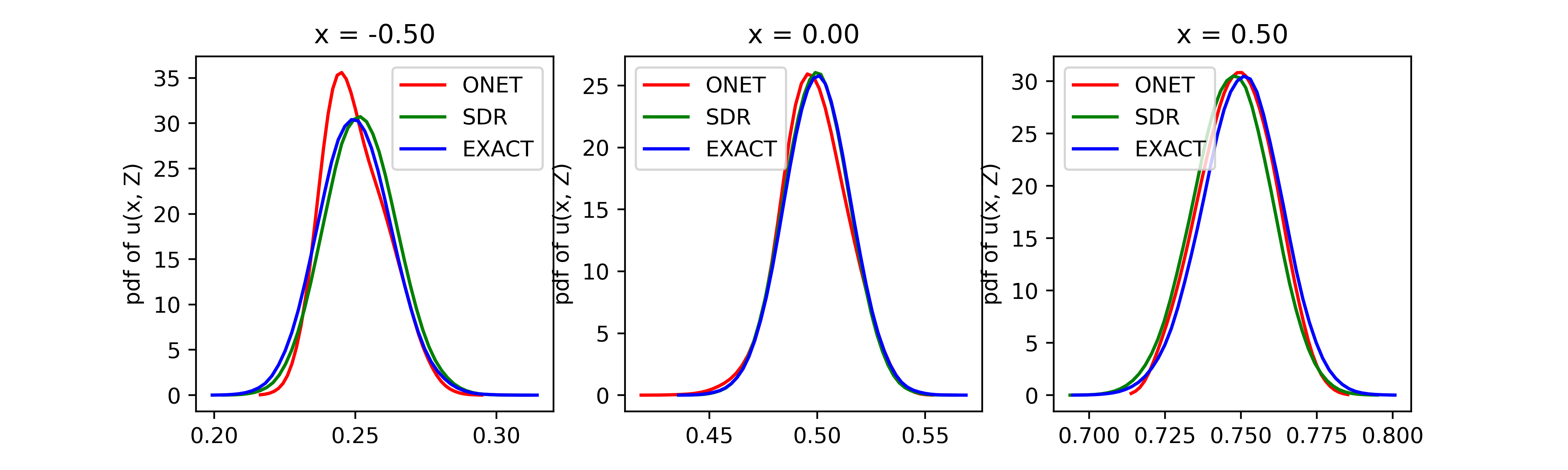
Figure 2: Marginal distributions of the solution to the 1d Dirichlet problem in Section 4.1. Left: the pdf of $u_{\theta}(x,Z)$ at $x=-0.5$; Center: the pdf of $u_{\theta}(x,Z)$ at $x=0$; Right: the pdf of $u_{\theta}(x,Z)$ at $x=0.5$.

Finally, we visualize the joint density for $(u_{\theta}(-0.5,Z),u_{\theta}(0.5,Z))$ in Figure 3, which verifies that the approximated solution $u_{\theta}(x,Z)$ captures the correct correlation of the random field at different $x$.

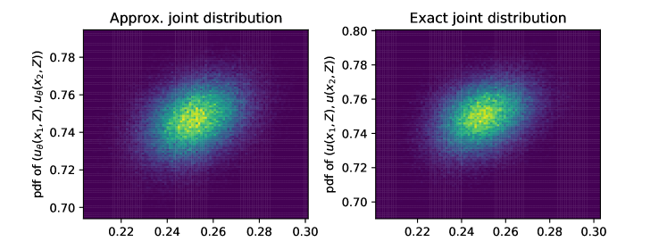
Figure 3: Joint distribution of the solution to the 1d Dirichlet problem in Section 4.1. Left: the approximated joint pdf of $u_{\theta}(-0.5,Z)$ and $u_{\theta}(0.5,Z)$; Right: the exact joint pdf $u(-0.5,Z)$ and $u(0.5,Z)$.

4.2 A quadratic Lagrangian with Neumann boundary condition

Next, we consider the following Lagrangian

$$I(x,u,\nabla u;\kappa)=\frac{1}{2}\kappa(x,Z)|\nabla u(x,Z)|^{2}-f(x,u(x,Z),Z)\ u(x,Z)$$ (10)

While we take $d$ arbitrary for now, $N=1$ is assumed. The physical domain is $D=[0,1]^{d}$. We impose the following Neumann boundary conditions on $\partial D$

$$\frac{\partial u}{\partial n}(x,Z)=0.$$

The random field $\kappa$ is taken to be

$$\kappa(x,Z)=d+1+\sum_{i=1}^{d}Z_{i}$$

with $Z=(Z_{1},\ldots,Z_{d})$ uniformly distributed over $D$ and the semilinear term $f$ is given by

$$f(x,u(x,Z),Z)=-\pi^{2}(d+1+\sum_{i=1}^{d}Z_{i})\ u(x,Z)+2\pi^{2}\sum_{i=1}^{d}\cos(\pi x_{i}).$$

It can be easily verified that the unique solution of the minimization problem (4) with the Lagrangian (10) is

$$u(x,Z)=\frac{1}{\kappa(x,Z)}\sum_{i=1}^{d}\cos(\pi x_{i}).$$

To solve the above minimization problem numerically, we approximate the solution $u(X,Z)$ by a DNN realization $u_{\theta}(X,Z)$ and formulate the following variational problem:

$$\min_{\theta}J(\theta)\quad\textrm{with}\quad J(\theta)=\mathbb{E}\left[\frac{1}{2}\left(\kappa(X,Z)|\nabla u_{\theta}(X,Z)|^{2}-f(X,u_{\theta}(X,Z),Z)u_{\theta}(X,Z)\right)\right].$$

Note that this problem does not require a penalty term and hence the ground truth remains unchanged.

In the numerical experiment with $d=2$, we use a $L=5$ layer fully-connected DNN with $W=32$ nodes in each layer and $\tanh$ activation. We train the DNN for $3\times 10^{5}$ iterations with a minibatch size $2560$ per iteration. The initial learning rate is set to $\eta=10^{-4}$ and is decayed by a factor of $0.1$ after every $10^{5}$ iterations. We test the accuracy of the trained DNN solution by computing the the relative $L^{2}$ mean error using a Monte Carlo integration. Based on $10^{4}$ test samples, the final relative $L^{2}$ mean error is $E(\theta)=0.65\%$. The decays of both the loss function $J(\theta)$ and the relative $L^{2}$ mean error $E(\theta)$ with respect to the number of iterations are visualized in Figure 4, which demonstrates a consistent convergence behavior of $J(\theta)$ and $E(\theta)$. These results confirm that minimizing the loss $J(\theta)$ leads to a good approximation to the true solution.

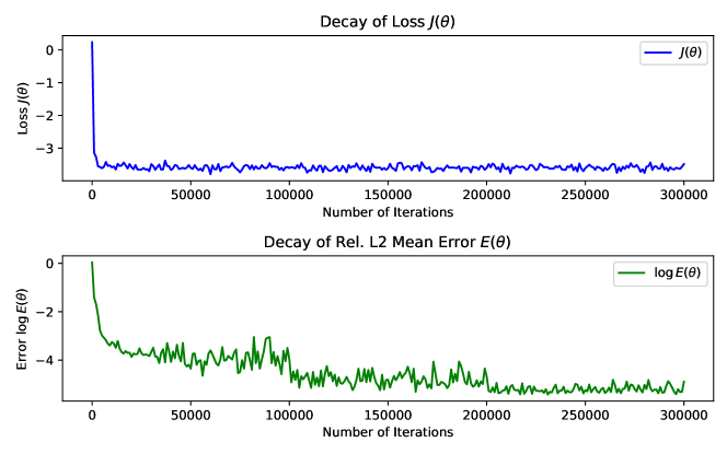
Figure 4: Convergence of the stochastic deep-Ritz applied to the Neumann problem in Section 4.2. Top: decay of the variational loss. Bottom: decay of the relative $L^{2}$ mean error (in log scale).

To demonstrate the distributional behavior of the DNN solution $u_{\theta}(X,Z)$, we compare its distribution to the distribution of the true solution $u(X,Z)$ at various values of $X$. The probability density functions (PDF) are shown in Figure 5. These results clearly indicate that the stochastic deep-Ritz solver is capable of capturing the distributional property of the true random field.

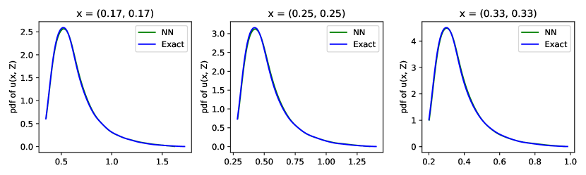
Figure 5: Marginal distributions of the solution to the $2$ dimensional Neumann problem in Section 4.2. Left: the pdf of $u_{\theta}(x,Z)$ at $x=(1/6,1/6)$; Center: the pdf of $u_{\theta}(x,Z)$ at $x=(1/4,1/4)$; Right: the pdf of $u_{\theta}(x,Z)$ at $x=(1/3,1/3)$.

We conclude this subsection by applying the stochastic deep-Ritz method to the Neumann problem (10) in $d=10$ dimensions. We employ the same DNN architecture, number of iterations and minibatch size as that for the case $d=2$. We set the initial learning rate to $\eta=10^{-5}$ and decay it after every $10^{5}$ iterations by a factor of 10. The final relative $L^{2}$ mean error $E(\theta)$ turns out to be $0.93\%$ and the numerical results for the marginal distributions $u_{\theta}(\cdot,Z)$ are presented in Figure 6. The results confirm that, with the same computational cost, the stochastic deep-Ritz method maintains the desired accuracy for high dimensional problems, a clear indication that the method may have the potential to overcome the curse of dimensionality.

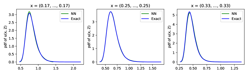
Figure 6: Marginal distributions of the solution to the $10$ dimensional Neumann problem in Section 4.2. Left: the pdf of $u_{\theta}(x,Z)$ at $x=(1/6,\ldots,1/6)\in\mathbb{R}^{10}$; Center: the pdf of $u_{\theta}(x,Z)$ at $x=(1/4,\ldots,1/4)\in\mathbb{R}^{10}$; Right: the pdf of $u_{\theta}(x,Z)$ at $x=(1/3,\ldots,1/3)\in\mathbb{R}^{10}$.

4.3 A quadratic Lagrangian with Dirichlet boundary condition

In this numerical example, we employ the Lagrangian (10) with $d=2$, $N=1$ and

$$f(x,u(x,Z),Z)=2\pi^{2}\sin(\pi x_{1})\sin(\pi x_{2}).$$

In contrast to the previous example, we take a zero boundary condition $u(x,Z)=0$ on $\partial D$. Here, the random field is defined as

$$\kappa(x,Z)=3+Z_{1}+Z_{2}$$

with $Z=(Z_{1},Z_{2})$ uniformly distributed over $[-1,1]^{2}$. The problem admits the unique solution

$$u(x,Z)=\frac{1}{\kappa(x,Z)}\sin(\pi x_{1})\sin(\pi x_{2}).$$

In order to solve the problem using DNN, we seek a minimizer of the loss function of the form (6).

The numerical experiment is carried out with a $L=5$ layer fully-connected DNN with $W=256$ nodes per layer and the tanh activation function. The DNN is trained for $4\times 10^{5}$ iterations using $2560$ samples per minibatch for each iteration We use a learning rate scheduling with the initial learning rate $\eta=10^{-3}$ and decay the learning rate by a factor of $10$ after every $10^{5}$ iterations. We plot the loss function $J(\theta)$ and the relative $L^{2}$ mean error $E(\theta)$ in Figure 7, which again demonstrates that $J(\theta)$ and $E(\theta)$ decay in a consistent manner. Note that there is a clear decrease of $E(\theta)$ after the first $10^{5}$ iterations due to the learning rate scheduling.

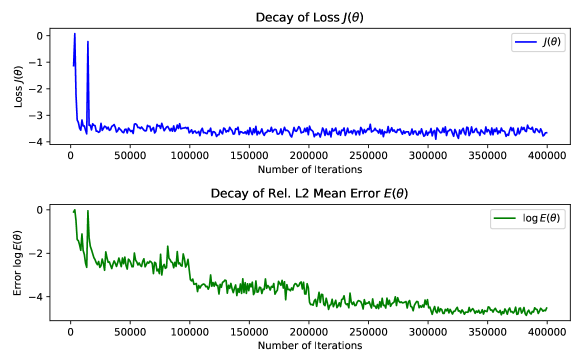
Figure 7: Convergence of the stochastic deep-Ritz applied to the Dirichlet problem. The first $1000$ iterations is skipped in the plot. Top: decay of the variational loss. Bottom: decay of the relative $L^{2}$ mean error (in log scale).

We gauge the accuracy of the DNN solution $u_{\theta}(x,Z)$ by comparing it to the exact solution $u(x,Z)$. With $10^{5}$ Monte Carlo test samples, the relative $L^{2}$ mean error is $E(\theta)=0.96\%$. To further assess the accuracy of the approximated solution $u_{\theta}(x,Z)$, we plot the marginal distribution and the joint distribution of the random field in Figure 8 and Figure 9, respectively. The numerical results suggest that the stochastic deep-Ritz method achieves a highly accurate approximation to the true solution.

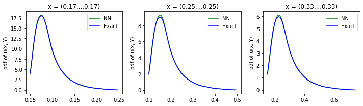
Figure 8: Distributions of the solution to the Dirichlet problem in Section 4.3 with penalty coefficient $\beta=500$. Left: the (unnormalized) pdf of $u_{\theta}(x,Z)$ at $x=(1/6,1/6)$; Center: the (unnormalized) pdf of $u_{\theta}(x,Z)$ at $x=(1/4,1/4)$; Right: the (unnormalized) pdf of $u_{\theta}(x,Z)$ at $x=(1/3,1/3)$.

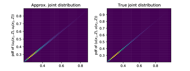
Figure 9: Joint distribution of the solution to the Dirichlet problem in Section 4.3 at $x_{1}=(-0.5,-0.5)$ and $x_{2}=(0.5,0.5)$. Left: the approximated joint pdf of $u_{\theta}(x_{1},Z)$ and $u_{\theta}(x_{2},Z)$; Right: the exact joint pdf $u(x_{1},Z)$ and $u(x_{2},Z)$.

4.4 Overdamped Langevin dynamics with Dirichlet boundary condition

As the final test problem, we consider the Lagrangian (10) with $N=1$, $f(x,Z)=-dZ$, and $\kappa(x,Z)=\textrm{e}^{-V(x,Z)}$, where

$$V(x,Z)=Z(1+\|x\|^{2})$$

We take $D$ to be the $d$-dimensional unit ball $B(0,1)$. In addition, $u(x,Z)=\textrm{e}^{Z}$ on $\partial D$ is assumed. The unique solution to the problem can be readily verified to be $u(x,Z)=\textrm{e}^{V}$.

Stochastic minimization of the loss function $J(\theta)$ associated with this problem involves uniform sampling in $B(0,1)$, which can be performed by standard rejection sampling. However, for high dimensional problems (e.g., $d=10$), the rejection sampling becomes infeasible due to the high rejection rate. We instead utilize the ball point picking algorithm to sample uniformly in $B(0,1)$ [49]. For the boundary penalty term this amounts to sampling a uniform random vector $S$ on the sphere $\partial B(0,1)$. We use the fact that

$$S=\frac{(X_{1},\ldots,X_{d})}{\sqrt{X_{1}^{2}+\ldots+X_{d}^{2}}}$$

is uniform on $\partial B(0,1)$ when $X_{1},\ldots,X_{d}$ are independent identically distributed standard normal random variables.

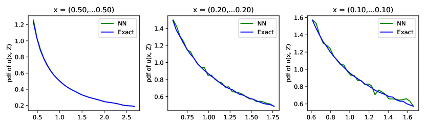
Figure 10: Marginal distributions of the solution to the problem in Section 4.4 with $d=4$ and penalty coefficient $\beta=500$. Left: the pdf of $u_{\theta}(x,Z)$ at $x=(0.5,\ldots,0.5)\in\mathbb{R}^{4}$; Center: the pdf of $u_{\theta}(x,Z)$ at $x=(0.2,\ldots,0.2)\in\mathbb{R}^{4}$; Right: the pdf of $u_{\theta}(x,Z)$ at $x=(0.1,\ldots,0.1)\in\mathbb{R}^{4}$.

The numerical experiments are carried out with $d=4$ and $d=10$. In both cases, we employ a $5$-layer fully-connected DNN with $W=256$ nodes per layer and we set mini-batch size to be $2560$. The training of the DNN takes $3\times 10^{5}$ iterations with an initial learning rate $\eta=10^{-3}$ that is decreased by a factor of $10$ after every $10^{5}$ iterations. Finally, we choose the penalty coefficient $\lambda=500$ to enforce the boundary condition. The numerical results for $d=4$ and for $d=10$ are presented in Figure 10 and Figure 11, respectively, displaying the distribution of the solution $u_{\theta}(x,Z)$ at different $x$. The relative $L^{2}$ mean errors are $E(\theta)=0.19\%$ for $d=4$ and $E(\theta)=0.43\%$ for $d=10$. The experiments, again, suggest that deep learning may overcome the curse of dimensionality exhibited by traditional discretization-based methods. However, we also observe that the solution becomes noisy in the high dimensional setting since the optimization problem becomes more challenging when $d$ is large.

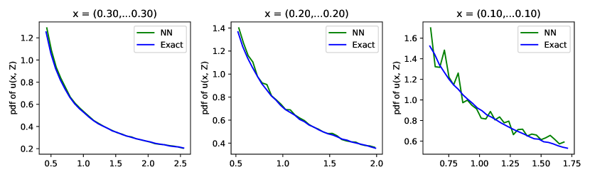
Figure 11: Marginal distributions of the solution to the problem in Section 4.4 with $d=10$. Left: the pdf of $u_{\theta}(x,Z)$ at $x=(0.3,\ldots,0.3)\in\mathbb{R}^{10}$; Center: the pdf of $u_{\theta}(x,Z)$ at $x=(0.2,\ldots,0.2)\in\mathbb{R}^{10}$; Right: the pdf of $u_{\theta}(x,Z)$ at $x=(0.1,\ldots,0.1)\in\mathbb{R}^{10}$.

Summary and Conclusion

In this article, we have presented a DNN-based method for solving stochastic variational problems through a combination of Monte Carlo sampling and DNN approximation. As an application, we mainly focused on the stochastic variational problem involving a quadratic functional.

Our method differs from traditional approaches for solving stochastic variational problems. First and foremost, the utilization of the DNN approximation and Monte Carlo sampling allows to avoid a discretization of the physical domain (e.g., finite element and finite volume) that often incurs an exponential growth of computational cost with the number of dimensions. Therefore, the method is applicable to problems with high dimensions in both physical space and stochastic space. Second, the stochastic variational formulation combined with DNN offers a natural loss function readily optimized by SGD methods. Moreover, the variational approach is well known to retain certain structures of the original problem and hence it is particularly advantageous when applied to structure preserving problems.

Despite the above benefits, our method does suffer from several limitations. From the theoretical viewpoint, the lack of convergence result of our method makes the hyperparameter tuning ad-hoc. This issue becomes particularly challenging for high-dimensional problems. From the practical viewpoint, the boundary condition penalization incorporated in the loss function alters the ground truth and hence limits the superior accuracy of the method. Lastly, the Monte Carlo sampling over a general domain $D$ can be quite challenging as it involves a constrained sampling over $D$ and $\partial D$. For a complex domain $D$ (e.g., with holes), the rejection sampling may become infeasible, especially in high dimension. In this case, an application of the constrained Markov chain Monte Carlo may be required [50, 51, 52, 53, 54].

Appendix A The quadratic Lagrangian setting

An important class of problems related to the stochastic variational problem (4) is the random coefficient elliptic equation (8). To recast (8) into a stochastic variational problem (3), we first set up an appropriate function space for the problem. We introduce the physical space $H_{0}^{1}(D)$, i.e., the Sobolev space of functions with weak derivatives up to order $1$ and vanishing on the boundary. To define the function space for $Z$, we assume that $Z$ admits a probability density function $\rho(z)$ so that

$$\mathbb{E}[g(Z(\omega))]=\int_{\Gamma}g(z)\rho(z)\,dz$$

for any measurable function $g:\Gamma\to\mathbb{R}$. Then we define the stochastic space $L_{\rho}^{2}(\Gamma)$, i.e.,

$$L_{\rho}^{2}(\Gamma)=\left\{g:\Gamma\to\mathbb{R}~{}\left|~{}\int_{\Gamma}|g(z)|^{2}\rho(z)\,dz<\infty\right.\right\},$$

which is the $\rho$-weighted $L^{2}$ space over $\Gamma$. The solution $u(x,Z)$ to (8) is thus defined in the space

$$L^{2}(\Gamma,H_{0}^{1}(D))=\left\{v:D\times\Gamma\to\mathbb{R}\left|~{}v\textrm{~{}is strongly measurable and~{}}\|v\|_{H_{0}^{1}(D)}\in L_{\rho}^{2}(\Gamma)\right.\right\},$$ (11)

where the norm $\|\cdot\|_{L^{2}(\Gamma,H_{0}^{1}(D))}$ is induced by the inner product:

$$\begin{split}\langle u,v\rangle&=\int_{\Gamma}\int_{D}u(x,z)v(x,z)\rho(z)\,dx\,dz+\int_{\Gamma}\int_{D}\nabla u(x,z)\cdot\nabla v(x,z)\rho(z)\,dx\,dz\\ &=\mathbb{E}\left[\int_{D}u(x,Z)v(x,Z)\,dx\right]+\mathbb{E}\left[\int_{D}\nabla u(x,Z)\cdot\nabla v(x,Z)\,dx\right].\end{split}$$ (12)

Under certain conditions, a direct application of the Lax-Milgram theorem immediately implies the well-posedness of the following stochastic weak form of (8):

$$\mathbb{E}\left[\int_{D}\kappa(x,Z)\nabla u(x,Z)\cdot\nabla v(x,Z)-f(x,Z)v(x,Z)\,dx\right]=0,\quad\forall v\in L^{2}(\Gamma,H_{0}^{1}(D)).$$ (13)

The above stochastic weak form is equivalent to a min-max problem which involves a saddle points searching. Therefore, it is possible to solve the problem using deep learning frameworks such as the generative adversarial network (GAN) and its variants [55, 56]. However, it is well known that training of GAN is a difficult task often requiring fine tuning of hyper-parameters. The training becomes even more challenging in the context of PDEs. We refer the reader to [57] for a recent work on solving deterministic PDEs using GAN.

Owing to the difficulty of training GAN models based on the stochastic weak form, we alternatively reformulate (8) into the following stochastic variational problem

$$\min_{u\in L^{2}(\Gamma,H_{0}^{1}(D))}J(u)\quad\textrm{with}\quad J(u)=\mathbb{E}\left[\int_{D}\frac{1}{2}\kappa(x,Z)|\nabla u(x,Z)|^{2}-f(x,Z)u(x,Z)\,dx\right].$$ (14)

This stochastic variational problem can be viewed as an extension of the Ritz formulation (or Dirichlet’s principle) to the stochastic setting. The following theorem provides the theoretical justification of the stochastic variational reformulation.

Theorem 1.

Under the following two assumptions:

1. The diffusivity coefficient $\kappa(x,Z)$ is uniformly bounded and uniformly coercive, i.e., there exist constants $0<\kappa_{\min}\leq\kappa_{\max}$ such that for almost all $\omega\in\Omega$,

   $$\mathbb{P}\left(\omega\in\Omega:\kappa_{\textrm{min}}\leq\kappa(x,Z(\omega))\leq\kappa_{\textrm{max}},~{}\forall x\in\bar{D}\right)=1.$$

2. The forcing $f(x,Z)$ satisfies the following integrability condition:

   $$\mathbb{E}\left[\int_{D}|f(x,Z)|^{2}\,dx\right]<\infty.$$

Then the stochastic variational problem (14) admits a minimizer $u^{*}\in L^{2}(\Gamma,H_{0}^{1}(D))$. Furthermore, $u^{*}$ satisfies the stochastic weak form (13).

Proof.

To show the existence of a minimizer $u^{*}$ to (14), it is sufficient to show that 1) there exists a minimizing sequence $u_{n}(x,Z)$ (up to a subsequence) that converges weakly to some $u^{*}\in L^{2}(\Gamma,H_{0}^{1}(D))$ and 2) the functional $J(u)$ is (weakly) lower semicontinuous [37].

Denote $J^{*}=\inf\{J(u)~{}|~{}u\in L^{2}(\Gamma,H_{0}^{1}(D))\}$. Note that $J^{*}>-\infty$ and hence there exists a minimizing sequence $u_{n}$ such that $J(u_{n})\to J^{*}$. We shall show that there exists $u^{*}\in L^{2}(\Gamma,H_{0}^{1}(D))$ such that $J^{*}=J(u^{*})$.

For weak convergence of the sequence $u_{n}(x,Z)$, it suffices to uniformly bound $u_{n}$ in $L^{2}(\Gamma,H_{0}^{1}(D))$. To this end, note that by the assumption on $\kappa$,

$$\frac{1}{2}\kappa(x,Z)|\nabla u_{n}(x,Z)|^{2}-f(x,Z)u_{n}(x,Z)\geq\frac{1}{2}\kappa_{\text{min}}|\nabla u_{n}(x,Z)|^{2}-f(x,Z)u_{n}(x,Z).$$

Integrating over $D$ and taking expectation of both sides lead to

$$J(u_{n})\geq\frac{1}{2}\kappa_{\text{min}}\mathbb{E}\left[\int_{D}|\nabla u_{n}(x,Z)|^{2}\,dx\right]-\mathbb{E}\left[\int_{D}f(x,Z)u_{n}(x,Z)\,dx\right].$$

Invoking the assumption on $\kappa$ and the Cauchy-Schwarz inequality leads to

$$J(u_{n})\geq C_{1}\mathbb{E}\left[||\nabla u_{n}(\cdot,Z)||_{L^{2}(D)}^{2}\right]-\mathbb{E}\left[\|f(\cdot,Z)\|_{L^{2}(D)}^{2}\right]^{\frac{1}{2}}\mathbb{E}\left[\|u_{n}(\cdot,Z)\|_{L^{2}(D)}^{2}\right]^{\frac{1}{2}},$$

where $C_{1}=\kappa_{\min}/2$. By the assumption on $f$ and the Poincaré’s inequality, there exists a constant $C_{2}>0$ (which depends on $f$ and the domain $D$) such that

$$J(u_{n})\leq C_{1}\mathbb{E}\left[||\nabla u_{n}(\cdot,Z)||_{L^{2}(D)}^{2}\right]-C_{2}\mathbb{E}\left[\|\nabla u_{n}(\cdot,Z)\|_{L^{2}(D)}^{2}\right]^{\frac{1}{2}}.$$

Now note that $J(u_{n})$ is uniformly bounded (in $n$) since it is a minimizing sequence of (14), which implies $\mathbb{E}\{\|\nabla u_{n}(\cdot,Z)\|_{L^{2}(D)}^{2}\}$ is uniformly bounded (in $n$) and hence

$$\sup_{n}\mathbb{E}\{\|u_{n}(\cdot,Z)\|_{H_{0}^{1}(D)}^{2}\}<\infty.$$

Therefore, there exists a subsequence, still denoted by $u_{n}$, that converges weakly to some $u^{*}\in L^{2}(\Gamma,H_{0}^{1}(D))$.

Next, we justify that $J(u)$ is (weakly) lower semicontinuous. For each $z\in\mathbb{R}^{K}$, define the functional $L_{z}:D\times\mathbb{R}\times\mathbb{R}^{n}\to\mathbb{R}$ by

$$L_{z}(x,u,\xi)=\frac{1}{2}\kappa(x,z)|\xi|^{2}+f(x,z)u.$$

Since $(u,\xi)\mapsto L_{z}(x,u,\xi)$ is convex for every $x$ and $z$, we have for all $x\in D$ and almost all $\omega\in\Omega$,

$$\begin{split}L_{Z(\omega)}(x,u_{n},\nabla u_{n})\geq L_{Z(\omega)}(x,u^{*},\nabla u^{*})&+\partial_{u}L_{Z(\omega)}(x,u^{*},\nabla u^{*})(u_{n}-u^{*})\\ &+\partial_{\xi}L_{Z(\omega)}(x,u^{*},\nabla u^{*})\cdot(\nabla u_{n}-\nabla u^{*}).\end{split}$$

Integrating both sides of the above inequality and then taking expectations lead to

$$J(u_{n})\geq J(u^{*})+\mathbb{E}\left[\int_{D}f(x,Z)(u_{n}-u^{*})\,dx\right]+\mathbb{E}\left[\int_{D}\kappa(x,Z)\nabla u^{*}\cdot(\nabla u_{n}-\nabla u^{*})\,dx\right].$$

Since $u_{n}$ converges weakly to $u^{*}$ in $L^{2}(\Gamma,H_{0}^{1}(D))$ and both $f(x,Z)$ and $\kappa(x,Z)\nabla u^{*}$ are in $L^{2}(\Gamma,H_{0}^{1}(D))$, we immediately have

$$\liminf_{n\to\infty}J(u_{n})\geq J(u^{*}).$$

Therefore, $J(u)$ is (sequentially weak) lower semicontinuous and hence $u^{*}$ is a minimizer by the direct method of calculus of variation.

It remains to be shown that $u^{*}$ satisfies the weak form (13). To this end, we consider the functional $J$ evaluated at $u^{*}+\epsilon v$ for every $v\in L^{2}(\Gamma,H_{0}^{1}(D))$. A simple calculation shows that the Gateaux derivative satisfies

$$\begin{split}\lim_{\epsilon\to 0}\frac{1}{\epsilon}(J(u^{*}+\epsilon v)-J(u^{*}))=\mathbb{E}\left[\int_{D}\kappa(x,Z)\nabla u^{*}\cdot\nabla v-f(x,Z)v\,dx\right].\end{split}$$

Since $u^{*}$ is a minimizer of $J$, the Gateaux derivative

$$\left.\frac{d}{d\epsilon}\right|_{\epsilon=0}J(u^{*}+\epsilon v)=0,$$

and hence the weak form (13). ∎

References

- [1] I. Babuška, F. Nobile, R. Tempone, A stochastic collocation method for elliptic partial differential equations with random input data, SIAM Journal on Numerical Analysis 45 (3) (2007) 1005–1034.
- [2] F. Nobile, R. Tempone, C. G. Webster, A sparse grid stochastic collocation method for partial differential equations with random input data, SIAM Journal on Numerical Analysis 46 (5) (2008) 2309–2345.
- [3] F. Nobile, R. Tempone, C. G. Webster, An anisotropic sparse grid stochastic collocation method for partial differential equations with random input data, SIAM Journal on Numerical Analysis 46 (5) (2008) 2411–2442.
- [4] I. Babuska, R. Tempone, G. E. Zouraris, Galerkin finite element approximations of stochastic elliptic partial differential equations, SIAM Journal on Numerical Analysis 42 (2) (2004) 800–825.
- [5] H. G. Matthies, A. Keese, Galerkin methods for linear and nonlinear elliptic stochastic partial differential equations, Computer methods in applied mechanics and engineering 194 (12-16) (2005) 1295–1331.
- [6] F. Y. Kuo, D. Nuyens, Application of quasi-monte carlo methods to elliptic pdes with random diffusion coefficients: a survey of analysis and implementation, Foundations of Computational Mathematics 16 (6) (2016) 1631–1696.
- [7] R. G. Ghanem, P. D. Spanos, Stochastic finite elements: a spectral approach, Courier Corporation, 2003.
- [8] M. D. Gunzburger, C. G. Webster, G. Zhang, Stochastic finite element methods for partial differential equations with random input data, Acta Numerica 23 (2014) 521–650.
- [9] D. Xiu, G. E. Karniadakis, The Wiener–Askey polynomial chaos for stochastic differential equations, SIAM journal on scientific computing 24 (2) (2002) 619–644.
- [10] D. Xiu, G. E. Karniadakis, Modeling uncertainty in flow simulations via generalized polynomial chaos, Journal of computational physics 187 (1) (2003) 137–167.
- [11] P. Grohs, F. Hornung, A. Jentzen, P. Von Wurstemberger, A proof that artificial neural networks overcome the curse of dimensionality in the numerical approximation of black-scholes partial differential equations, arXiv preprint arXiv:1809.02362 (2018).
- [12] T. Poggio, H. Mhaskar, L. Rosasco, B. Miranda, Q. Liao, Why and when can deep-but not shallow-networks avoid the curse of dimensionality: a review, International Journal of Automation and Computing 14 (5) (2017) 503–519.
- [13] M. Raissi, P. Perdikaris, G. E. Karniadakis, Physics-informed neural networks: A deep learning framework for solving forward and inverse problems involving nonlinear partial differential equations, Journal of Computational physics 378 (2019) 686–707.
- [14] M. Raissi, P. Perdikaris, G. E. Karniadakis, Physics informed deep learning (part i): Data-driven solutions of nonlinear partial differential equations, arXiv preprint arXiv:1711.10561 (2017).
- [15] J. Sirignano, K. Spiliopoulos, Dgm: A deep learning algorithm for solving partial differential equations, Journal of computational physics 375 (2018) 1339–1364.
- [16] J. Berg, K. Nyström, A unified deep artificial neural network approach to partial differential equations in complex geometries, Neurocomputing 317 (2018) 28–41.
- [17] G. Carleo, M. Troyer, Solving the quantum many-body problem with artificial neural networks, Science 355 (6325) (2017) 602–606.
- [18] J. Han, A. Jentzen, et al., Deep learning-based numerical methods for high-dimensional parabolic partial differential equations and backward stochastic differential equations, Communications in Mathematics and Statistics 5 (4) (2017) 349–380.
- [19] J. Han, A. Jentzen, E. Weinan, Solving high-dimensional partial differential equations using deep learning, Proceedings of the National Academy of Sciences 115 (34) (2018) 8505–8510.
- [20] C. Beck, A. Jentzen, et al., Machine learning approximation algorithms for high-dimensional fully nonlinear partial differential equations and second-order backward stochastic differential equations, Journal of Nonlinear Science 29 (4) (2019) 1563–1619.
- [21] J. Han, et al., Deep learning approximation for stochastic control problems, arXiv preprint arXiv:1611.07422 (2016).
- [22] N. Nüsken, L. Richter, Solving high-dimensional hamilton–jacobi–bellman pdes using neural networks: perspectives from the theory of controlled diffusions and measures on path space, Partial Differential Equations and Applications 2 (4) (2021) 1–48.
- [23] N. Nüsken, L. Richter, Interpolating between bsdes and pinns–deep learning for elliptic and parabolic boundary value problems, arXiv preprint arXiv:2112.03749 (2021).
- [24] B. Yu, E. Weinan, The deep ritz method: a deep learning-based numerical algorithm for solving variational problems, Communications in Mathematics and Statistics 6 (1) (2018) 1–12.
- [25] Y. Khoo, J. Lu, L. Ying, Solving for high-dimensional committor functions using artificial neural networks, Research in the Mathematical Sciences 6 (1) (2019) 1–13.
- [26] Y. Khoo, J. Lu, L. Ying, Solving parametric pde problems with artificial neural networks, European Journal of Applied Mathematics 32 (3) (2021) 421–435.
- [27] J. Müller, M. Zeinhofer, Deep ritz revisited, arXiv preprint arXiv:1912.03937 (2019).
- [28] H. Li, L. Ying, A semigroup method for high dimensional elliptic pdes and eigenvalue problems based on neural networks, Journal of Computational Physics (2022) 110939.
- [29] C. Beck, M. Hutzenthaler, A. Jentzen, B. Kuckuck, An overview on deep learning-based approximation methods for partial differential equations, arXiv preprint arXiv:2012.12348 (2020).
- [30] E. Weinan, J. Han, A. Jentzen, Algorithms for solving high dimensional pdes: From nonlinear monte carlo to machine learning, Nonlinearity 35 (1) (2021) 278.
- [31] E. Weinan, Machine learning and computational mathematics, arXiv preprint arXiv:2009.14596 (2020).
- [32] Y. Zhu, N. Zabaras, P.-S. Koutsourelakis, P. Perdikaris, Physics-constrained deep learning for high-dimensional surrogate modeling and uncertainty quantification without labeled data, Journal of Computational Physics 394 (2019) 56–81.
- [33] X. Zhang, K. Garikipati, Bayesian neural networks for weak solution of pdes with uncertainty quantification, arXiv preprint arXiv:2101.04879 (2021).
- [34] L. Lu, P. Jin, G. E. Karniadakis, Deeponet: Learning nonlinear operators for identifying differential equations based on the universal approximation theorem of operators, arXiv preprint arXiv:1910.03193 (2019).
- [35] Z. Li, N. Kovachki, K. Azizzadenesheli, B. Liu, K. Bhattacharya, A. Stuart, A. Anandkumar, Fourier neural operator for parametric partial differential equations, arXiv preprint arXiv:2010.08895 (2020).
- [36] S. H. Mariano Giaquinta, Calculus of Variations I, Springer Berlin Heidelberg, 2013.
- [37] B. Dacorogna, Direct methods in the calculus of variations, Vol. 78, Springer Science & Business Media, 2007.
- [38] T. Wang, J. Knap, Stochastic gradient descent for semilinear elliptic equations with uncertainties, Journal of Computational Physics 426 (2021) 109945.
- [39] K. He, X. Zhang, S. Ren, J. Sun, Deep residual learning for image recognition, in: Proceedings of the IEEE conference on computer vision and pattern recognition, 2016, pp. 770–778.
- [40] O. Ronneberger, P. Fischer, T. Brox, U-net: Convolutional networks for biomedical image segmentation, in: Medical Image Computing and Computer-Assisted Intervention–MICCAI 2015: 18th International Conference, Munich, Germany, October 5-9, 2015, Proceedings, Part III 18, Springer, 2015, pp. 234–241.
- [41] L. Lu, R. Pestourie, W. Yao, Z. Wang, F. Verdugo, S. G. Johnson, Physics-informed neural networks with hard constraints for inverse design, SIAM Journal on Scientific Computing 43 (6) (2021) B1105–B1132.
- [42] L. Sun, H. Gao, S. Pan, J.-X. Wang, Surrogate modeling for fluid flows based on physics-constrained deep learning without simulation data, Computer Methods in Applied Mechanics and Engineering 361 (2020) 112732.
- [43] J. Müller, M. Zeinhofer, Notes on exact boundary values in residual minimisation, arXiv preprint arXiv:2105.02550 (2021).
- [44] S. Asmussen, P. W. Glynn, Stochastic simulation: algorithms and analysis, Vol. 57, Springer, 2007.
- [45] P. Glasserman, Monte Carlo methods in financial engineering, Vol. 53, Springer, 2004.
- [46] M. Struwe, Variational methods, Vol. 31999, Springer, 1990.
- [47] D. P. Kingma, J. Ba, Adam: A method for stochastic optimization, arXiv preprint arXiv:1412.6980 (2014).
- [48] A. Paszke, S. Gross, S. Chintala, G. Chanan, E. Yang, Z. DeVito, Z. Lin, A. Desmaison, L. Antiga, A. Lerer, Automatic differentiation in pytorch (2017).
- [49] F. Barthe, O. Guédon, S. Mendelson, A. Naor, A probabilistic approach to the geometry of the -ball, The Annals of Probability 33 (2) (2005) 480–513.
- [50] W. Zhang, Ergodic sdes on submanifolds and related numerical sampling schemes, ESAIM: Mathematical Modelling and Numerical Analysis 54 (2) (2020) 391–430.
- [51] G. Ciccotti, T. Lelievre, E. Vanden-Eijnden, Projection of diffusions on submanifolds: Application to mean force computation, Communications on Pure and Applied Mathematics: A Journal Issued by the Courant Institute of Mathematical Sciences 61 (3) (2008) 371–408.
- [52] T. Lelievre, M. Rousset, G. Stoltz, Langevin dynamics with constraints and computation of free energy differences, Mathematics of computation 81 (280) (2012) 2071–2125.
- [53] E. Zappa, M. Holmes-Cerfon, J. Goodman, Monte carlo on manifolds: sampling densities and integrating functions, Communications on Pure and Applied Mathematics 71 (12) (2018) 2609–2647.
- [54] T. Lelièvre, M. Rousset, G. Stoltz, Hybrid monte carlo methods for sampling probability measures on submanifolds, Numerische Mathematik 143 (2) (2019) 379–421.
- [55] I. Goodfellow, J. Pouget-Abadie, M. Mirza, B. Xu, D. Warde-Farley, S. Ozair, A. Courville, Y. Bengio, Generative adversarial nets, Advances in neural information processing systems 27 (2014).
- [56] M. Arjovsky, S. Chintala, L. Bottou, Wasserstein generative adversarial networks, in: International conference on machine learning, PMLR, 2017, pp. 214–223.
- [57] Y. Zang, G. Bao, X. Ye, H. Zhou, Weak adversarial networks for high-dimensional partial differential equations, Journal of Computational Physics 411 (2020) 109409.