Comment on the subtlety of defining real-time path integral in lattice gauge theories

Nobuyuki Matsumoto

RIKEN/BNL Research center, Brookhaven National Laboratory, Upton, NY 11973, USA

Recently, Hoshina, Fujii, and Kikukawa pointed out that the naive lattice gauge theory action in Minkowski signature does not result in a unitary theory in the continuum limit, and Kanwar and Wagman proposed alternative lattice actions to the Wilson action without divergences. We here show that the subtlety can be understood from the asymptotic expansion of the modified Bessel function, which has been discussed for path integral of compact variables in nonrelativistic quantum mechanics. The essential ingredient for defining the appropriate continuum theory is the $i\varepsilon$ prescription, and with the proper implementation of the $i\varepsilon$ we show that the Wilson action can be used for the real-time path integrals. It is here important that the $i\varepsilon$ should be implemented for both timelike and spacelike plaquettes. We also argue the reason why the $i\varepsilon$ becomes required for the Wilson action from the Hamiltonian formalism. The $i\varepsilon$ is needed to manifestly suppress the contributions from singular paths, for which the Wilson action can give different values from those of the actual continuum action.

1 Introduction

Real-time path integral [1] has recently been revisited both analytically [2, 3, 4] and numerically [5, 6, 7, 8, 9, 10, 11, 12] for the interest of real-time dynamics in quantum theories. Especially in the numerical side, many developments have been made to tame the infamous sign problem (e.g., complex Langevin [13, 14, 5, 6, 15, 16], contour deformation techniques including Lefschetz thimble methods [2, 17, 18, 19, 3, 20, 7, 21, 22, 8, 9, 23, 24, 25, 26, 27, 28, 29, 30, 11], and tensor renormalization group [31, 32, 33, 34, 35, 36, 37, 38, 39, 10, 40]), which can enables us to investigate real-time quantum systems via numerical calculation. It is thus becoming not only of theoretical interest but also of practical importance to establish an appropriate way to calculate the real-time path integrals. Recently, Hoshina, Fujii, and Kikukawa [41] pointed out that the naive lattice gauge theory action in Minkowski signature does not result in a unitary theory in the continuum limit, and Kanwar and Wagman [30] proposed alternative lattice actions to the Wilson action removing divergences to give a well-defined continuum limit. In this paper, we point out that the subtlety can be understood from the asymptotic expansion of the modified Bessel function, which has been discussed in nonrelativistic quantum mechanics of compact variables [43, 44]. To get rid of the unwanted part of the asymptotic expansion, we need to incorporate the $i\varepsilon$ prescription, i.e., an infinitesimal Wick rotation [45]. The first point of this paper is that we can use the Wilson action for the numerical studies, but with the $i\varepsilon$ implemented. It is also possible to expand the Boltzmann weight with the characters to define the real-time action, in which case we express the characters not with the modified Bessel functions themselves but with its asymptotic expansion in $\varepsilon\rightarrow+0$. In the latter case, the $i\varepsilon$ is already built in the action, and thus, safely setting $\varepsilon=0$, the theory has an appropriate continuum limit.

In the above two actions, the key ingredient is the $i\varepsilon$, which we know is essential in the continuum theory to obtain the causal structure of the Green functions. However, it may seem uncertain why such $i\varepsilon$ is required without knowing the actual continuum quantum theory. As the second point of this paper, starting from the Hamiltonian formalism, we argue the reason why the $i\varepsilon$ becomes required for the Wilson action. Note that, the Wilson action is only guaranteed to reproduce the action values of the continuum action for smooth field configurations. Here, the $i\varepsilon$ is needed to manifestly suppress the contributions from these singular paths in the path integral.

As an illustrative example, we begin with a simple one-dimensional quantum mechanical system in a periodic box [30]. We define the lattice action by discretizing time direction resulting in a $U(1)$ theory, and review the subtlety in defining continuum limit of the real-time path integral for this model [43, 44, 30]. We in particular explain how the correct continuum limit emerges with the $i\varepsilon$ by analyzing the asymptotic expansion of the modified Bessel function [43]. We then argue the meaning of the $i\varepsilon$ by deriving the path integral from the Hamiltonian formalism. This model gives the essential structure for the necessity of the $i\varepsilon$.

With the detailed picture in quantum mechanics, the lattice gauge field theory can be seen in a straightforward manner. We first describe the subtlety of real-time path integral in gauge theories [30] with the modified Bessel function. The expansion of the Boltzmann weight with characters shows that we need to incorporate the $i\varepsilon$ both for the timelike and spacelike plaquettes. Next, we exemplify that the Wilson action can be used with the $i\varepsilon$ by using the two-dimensional $SU(2)$ and $SU(3)$ theories. Lastly, we argue the meaning of the $i\varepsilon$ from the Hamiltonian formalism, in particular considering the $SU(2)$ Wilson theory [46].

The remaining part of this paper is organized as follows. In section 2, we first review the subtlety of real-time path integral in the quantum mechanics on $S^{1}$. We then argue the meaning of the $i\varepsilon$ by deriving the path integral expression from the Hamiltonian formalism. In section 3, we move to the lattice gauge theory case. After describing the subtlety of the real-time path integral similarly to section 2, we demonstrate that the Wilson action can be used with the $i\varepsilon$. Lastly, we clarify the meaning of the $i\varepsilon$ in gauge theory from the Hamiltonian formalism. Section 4 is devoted to the conclusion and outlook.

2 Quantum mechanics example

In this section, we describe the subtlety in defining the real-time path integral of the quantum mechanics on $S^{1}$. This model has the subtlety of defining real-time path integral that is similar to lattice gauge theories [30].

2.1 Subtlety of real-time path integral in quantum mechanics on $S^{1}$

We consider a one-dimensional quantum system with the action:

$$S[\phi]\equiv\frac{\beta}{2}\int_{0}^{T}dt\,(\partial_{t}\phi)^{2},$$ (2.1)

where $\phi(t)$ is the angular variable on $S^{1}$. This model is equivalent to the ordinary one-dimensional quantum mechanics in a periodic box (see, e.g., [47, 48, 49, 50, 51, 52, 53]) by the identification

$$x(t)\equiv{L\over 2\pi}\phi(t),$$ (2.2)

where $L$ is the spatial extent of the system and $\beta$ gives the particle mass $(2\pi)^{2}\beta/L^{2}$. We here concentrate on the free case for simplicity. The corresponding Hamiltonian of the system is

$$H\equiv\frac{1}{2\beta}p_{\phi}^{2},$$ (2.3)

where $p_{\phi}$ is the conjugate momentum of $\phi$. In quantum mechanics, the plane waves $\{\exp(in\phi)\}_{n\in\mathbb{Z}}$ are the eigenfunctions of the momentum operator, which in this case diagonalize the Hamiltonian with the energy levels:

$$E_{n}\equiv\frac{1}{2\beta}n^{2}.$$ (2.4)

To define the path integral, we discretize the time $T=Na$ and introduce the $U(1)$ variables $U_{\ell}\equiv e^{i\phi_{\ell}}$, where $\phi_{\ell}=\phi(a\ell)$ $(\ell=0,\cdots,N)$. The transition amplitude from level $n_{i}$ to $n_{f}$:

$$A_{n_{f},n_{i}}(T) \equiv\langle n_{f}|e^{-i\hat{H}T}|n_{i}\rangle$$ (2.5)

may be expressed on the lattice naively as:

$$A^{\rm(lat)}_{n_{f},n_{i}}(T)\equiv{\cal N}\int(dU)\,e^{iS(U)}(U_{N}^{*})^{n_{f}}U_{0}^{n_{i}},$$ (2.6)

where

$$(dU) \equiv\prod_{\ell=0}^{N}dU_{\ell}\equiv\prod_{\ell=0}^{N}\frac{d\phi_{\ell}}{2\pi},$$ (2.7)

$$S(U) \equiv\frac{\beta}{2a}\sum_{\ell=0}^{N-1}|U_{\ell+1}-U_{\ell}|^{2}=-{\beta\over a}\sum_{\ell=0}^{N-1}{\rm Re}(U_{\ell+1}U_{\ell}^{*})+{\rm const}.$$ (2.8)

The normalization factor ${\cal N}$ can be determined by demanding $A^{\rm(lat)}_{n_{f},n_{i}}(0)=\delta_{n_{f},n_{i}}$.

To obtain the analytic expression of $A^{\rm(lat)}_{n_{f},n_{i}}(T)$, we expand the exponential in terms of characters:

$$e^{-i(\beta/a){\rm Re}\,U}=\sum_{n\in\mathbb{Z}}I_{n}\Big{(}{-i\beta\over a}\Big{)}U^{n},$$ (2.9)

where $I_{n}(\beta)$ is the modified Bessel function of the first kind. The integration in (2.6) can be performed analytically to give:

$$A^{\rm(lat)}_{n_{f},n_{i}}(T) ={\cal N}\delta_{n_{f},n_{i}}I^{N}_{n_{f}}\Big{(}{-i\beta\over a}\Big{)}.$$ (2.10)

The function $A^{\rm(lat)}_{n_{f},n_{i}}(T)$ is an analytic function of the coupling $\beta$ for finite $a$; however, it is not in the limit $a\rightarrow 0$. This can be seen in the asymptotic expansion of $I_{n}(z)$ for $|z|\rightarrow\infty$ [43]:

$$I_{n}(z) \sim\frac{e^{z}}{\sqrt{2\pi z}}\sum_{k\geq 0}\frac{\Gamma(n+k+1/2)}{k!\,\Gamma(n-k+1/2)}\Big{(}\frac{-1}{2z}\Big{)}^{k}$$

$$~{}~{}~{}\pm ie^{\pm in\pi}\frac{e^{-z}}{\sqrt{2\pi z}}\sum_{k\geq 0}\frac{\Gamma(n+k+1/2)}{k!\,\Gamma(n-k+1/2)}\Big{(}\frac{1}{2z}\Big{)}^{k}.$$ (2.11)

The plus signature applies for $-\pi/2<{\arg}z<3\pi/2$, and the negative signature for $-3\pi/2<{\arg}z<\pi/2$. For $|{\arg}\,z|<\pi/2$, including the imaginary-time case (${\arg}\,z=0$), the second term will be completely irrelevant because of the exponential factor. However, at ${\arg}\,z=-\pi/2$, which is the case for eq. (2.10), the second term also contributes equally to the first term. Therefore, the result will be different depending on how we approach the real-time continuum limit. To get the correct continuum limit, one can modify the kinetic term [43, 44] by introducing a slight imaginary part

$$\beta\rightarrow e^{i\varepsilon}\beta\quad(\varepsilon>0).$$ (2.12)

We first take the $a\rightarrow 0$ limit keeping $\varepsilon$ finite, and then take the $\varepsilon\rightarrow+0$ limit. In fact, for $|{\arg}z|<\pi/2$,

$$I_{n}(z)/I_{0}(z)\sim 1-\frac{n^{2}}{2}{1\over z}+\cdots,$$ (2.13)

which in our case gives

$$\bigg{[}I_{n}\Big{(}\frac{-ie^{i\varepsilon}\beta}{a}\Big{)}/I_{0}\Big{(}\frac{-ie^{i\varepsilon}\beta}{a}\Big{)}\bigg{]}^{N}\sim\Big{[}1-ie^{-i\varepsilon}\frac{n^{2}}{2}{a\over\beta}+\cdots\Big{]}^{N}\xrightarrow{a\rightarrow 0}\exp\Big{[}-ie^{-i\varepsilon}\frac{n^{2}t}{2\beta}\Big{]}.$$ (2.14)

Therefore,

$$A^{\rm(lat)}_{n_{f},n_{i}}(T)\xrightarrow{a\rightarrow 0}\delta_{n_{f},n_{i}}\exp\big{[}-ie^{-i\varepsilon}E_{n_{f}}T\big{]}\xrightarrow{\varepsilon\rightarrow+0}\delta_{n_{f},n_{i}}\exp\big{[}-iE_{n_{f}}T\big{]},$$ (2.15)

which is the desired real-time amplitude.

Note that we will not obtain the correct continuum amplitude if we take $a\rightarrow 0$ exactly on $\varepsilon=0$ [30]. In this case, the amplitude $A^{\rm(lat)}_{n_{f},n_{i}}(T)$ becomes a singular function with a highly oscillatory behavior because of the second term in eq. (2.11).

2.2 $i\varepsilon$ in the derivation of the path integral

Although the argument in subsection 2.1 is mathematically correct, it may be uncertain why such $i\varepsilon$ becomes required to obtain the correct continuum theory for the discretized action (2.8). In this subsection, we argue that, starting from the Hamiltonian formalism, we can understand the role of the $i\varepsilon$ as manifestly suppressing the contributions from singular paths, for which the discretized action can give different values from those of the actual continuum action.

We consider the Feynman kernel for an infinitesimal time increment $a$:

$$\langle U^{\prime}|e^{-ia\hat{H}}|U\rangle,$$ (2.16)

where $|U\rangle$ is the eigenstate of the unitary operator $\hat{U}$, $\hat{U}|U\rangle=U|U\rangle$, that satisfies the commutation relation:

$$[\hat{U},\hat{p}_{\phi}]=\hat{U}.$$ (2.17)

By inserting the momentum eigenstates $|n\rangle$:

$$\langle U|n\rangle\equiv U^{n}\quad(n\in\mathbb{Z}),$$ (2.18)

we have

$$\langle U^{\prime}|e^{-ia\hat{H}}|U\rangle =\sum_{n\in\mathbb{Z}}\exp\Big{[}\frac{-ia}{2\beta}n^{2}+in(\phi^{\prime}-\phi)\Big{]}$$

$$=e^{i\pi/4}\sqrt{\frac{2\pi\beta}{-a}}\sum_{w\in\mathbb{Z}}\exp\Big{[}i\frac{\beta(\phi^{\prime}-\phi+2\pi w)^{2}}{2a}\Big{]},$$ (2.19)

where we write $U=\exp(i\phi)$, $U^{\prime}=\exp(i\phi^{\prime})$ with $\phi,\phi^{\prime}\in[-\pi,\pi)$ and have used the Poisson summation formula to obtain the second line. Although the kernel (2.19) is not well-defined as an ordinary function because the theta function

$$\vartheta(v,\tau)\equiv\sum_{n\in\mathbb{Z}}e^{\pi in^{2}\tau}e^{2\pi inv}$$ (2.20)

is only analytic for ${\rm Im}\,\tau>0$, the kernel has a definite meaning as a distribution. To see this, it should be sufficient to check the Fourier integral in which the kernel is multiplied by the plane waves because all the state vectors can be expressed as a linear combination of these basis vectors. For the kernel (2.19), we trivially obtain

$$\int dU^{\prime}\,({U^{\prime}}^{*})^{n}\langle U^{\prime}|e^{-ia\hat{H}}|U\rangle=(U^{*})^{n}e^{-\frac{ia}{2\beta}n^{2}},$$ (2.21)

which is a well-defined number for given $n$ and $U$, and thus establishes the definite meaning of the kernel as a distribution.

We can now understand the need of $i\varepsilon$ discussed in section 2.1 with distributional terms. In fact, the naive real-time path integral in section 2.1 amounts to replacing the kernel (2.19) by the expression:

$$\langle U^{\prime}|e^{-ia\hat{H}}|U\rangle\to e^{i\pi/4}\sqrt{\frac{2\pi\beta}{-a}}\exp\Big{[}\frac{i\beta}{a}\big{[}1-{\rm Re}\,(U{U^{\prime}}^{*})\big{]}\Big{]}.$$ (2.22)

This replacement cannot be justified as a distributional relation because, as in section 2.1, the Fourier integral gives

$$\int dU^{\prime}\,({U^{\prime}}^{*})^{n}e^{i\pi/4}\sqrt{\frac{2\pi\beta}{-a}}\exp\Big{[}\frac{i\beta}{a}\big{[}1-{\rm Re}\,(U{U^{\prime}}^{*})\big{]}\Big{]}$$

$$=e^{i\pi/4}\sqrt{\frac{2\pi\beta}{-a}}e^{-in\phi}e^{i\beta/a}I_{n}\Big{(}\frac{-i\beta}{a}\Big{)}$$

$$\sim e^{-in\phi}\big{[}e^{\frac{-ia}{2\beta}(n^{2}-\frac{1}{4})}-i(-1)^{n}e^{\frac{2i\beta}{a}}e^{\frac{ia}{2\beta}(n^{2}-\frac{1}{4})}\big{]},$$ (2.23)

which has the $n$ and $\phi$ dependent second term. However, the first term has the correct $n$ and $\phi$ dependence, and the second term can be removed by the $i\varepsilon$. We thus have the distributional identity after correcting the shift of the zero-point energy:

$$\langle U^{\prime}|e^{-ia\hat{H}}|U\rangle=\lim_{\varepsilon\rightarrow+0}e^{\frac{-ia}{8e^{i\varepsilon\beta}}}e^{i\pi/4}\sqrt{\frac{2\pi e^{i\varepsilon}\beta}{-a}}\exp\Big{[}\frac{ie^{i\varepsilon}\beta}{a}\big{[}1-{\rm Re}\,(U{U^{\prime}}^{*})\big{]}\Big{]}.$$ (2.24)

This justifies the use of the discretized action (2.8) under the $i\varepsilon$. The rest of this section is devoted to systematically deriving this distributional equality.

We begin with introducing the $i\varepsilon$ and regarding the original kernel (2.19) as the $\varepsilon\to+0$ limit:

$$\langle U^{\prime}|e^{-ia\hat{H}}|U\rangle=\lim_{\varepsilon\rightarrow+0}\langle U^{\prime}|e^{-ia\hat{H}}|U\rangle\big{|}_{\beta\to e^{i\varepsilon}\beta}.$$ (2.25)

The expression inside the limit now becomes a well-defined function, and has a sharp peak around $U=U^{\prime}$ for an infinitesimal $a$. This allows us to rewrite the expression as

$$\langle U^{\prime}|e^{-ia\hat{H}}|U\rangle|_{\beta\to e^{i\varepsilon}\beta}\approx e^{i\pi/4}\sqrt{\frac{2\pi e^{i\varepsilon}\beta}{-a}}\exp\Big{(}\frac{ie^{i\varepsilon}\beta}{2a}\lfloor\phi^{\prime}-\phi\rfloor^{2}\Big{)},$$ (2.26)

where the function $\lfloor\cdot\rfloor$ returns the value in $[-\pi,\pi)$ modulo $2\pi$. Relation (2.26) becomes a distributional equality for an infinitesimal $a$ because the contributions with nontrivial winding are exponentially suppressed thanks to $\varepsilon>0$.

On the other hand, the kernel

$$\exp\Big{[}\frac{ie^{i\varepsilon}\beta}{a}\big{[}1-{\rm Re}\,(U{U^{\prime}}^{*})\big{]}\Big{]}=\exp\Big{[}\frac{ie^{i\varepsilon}\beta}{a}\big{[}1-\cos(\phi-\phi^{\prime})\big{]}\Big{]}$$ (2.27)

has a similar functional dependence to eq. (2.26); the function (2.27) has a sharp peak around $U=U^{\prime}$ for an infinitesimal $a$, which allows us to expand the cosine in powers of $\lfloor\phi-\phi^{\prime}\rfloor$ and convert the Fourier integral to a Gaussian integral:

$$\int_{-\pi}^{\pi}\frac{d\phi^{\prime}}{2\pi}\,e^{-in\phi^{\prime}}\exp\Big{[}\frac{ie^{i\varepsilon}\beta}{a}\big{[}1-\cos(\phi-\phi^{\prime})\big{]}\Big{]}$$

$$=\int_{-\pi}^{\pi}\frac{d\phi^{\prime}}{2\pi}\,e^{-in\phi^{\prime}}\exp\Big{[}\frac{ie^{i\varepsilon}\beta}{2a}\lfloor\phi-\phi^{\prime}\rfloor^{2}-\frac{ie^{i\varepsilon}\beta}{24a}\lfloor\phi-\phi^{\prime}\rfloor^{4}+\cdots\Big{]}$$

$$\approx e^{-in\phi}e^{-\frac{ia}{2\beta}n^{2}}\int_{-\infty}^{\infty}\frac{d\phi^{\prime\prime}}{2\pi}\,\exp\Big{[}\frac{ie^{i\varepsilon}\beta}{2a}{\phi^{\prime\prime}}^{2}\Big{]}\Big{(}1-\frac{ie^{i\varepsilon}\beta}{24a}{\phi^{\prime\prime}}^{4}+\cdots\Big{)}.$$ (2.28)

We see the desired $n$ and $\phi$ dependence in front of the Gaussian integral. The remaining integral only gives an overall constant that includes the shift of the zero-point energy:

$$\int_{-\infty}^{\infty}\frac{d\phi^{\prime\prime}}{2\pi}\,\exp\Big{[}\frac{ie^{i\varepsilon}\beta}{2a}{\phi^{\prime\prime}}^{2}\Big{]}\Big{(}1-\frac{ie^{i\varepsilon}\beta}{24a}{\phi^{\prime\prime}}^{4}+\cdots\Big{)} =\Big{(}1+\frac{ia}{8e^{i\varepsilon}\beta}+\cdots\Big{)}\sqrt{\frac{-a}{2\pi ie^{i\varepsilon}\beta}}$$

$$\sim\exp\Big{(}\frac{ia}{8e^{i\varepsilon}\beta}\Big{)}\sqrt{\frac{-a}{2\pi ie^{i\varepsilon}\beta}}.$$ (2.29)

Correcting this constant gives the distributional relation (2.24).

Note the ordering of the limit. The distributional relation (2.24) is for an infinitesimal $a$ and for $\varepsilon>0$, and thus we first take the $a\rightarrow 0$ limit keeping $\varepsilon>0$. Correspondingly, we take the $\varepsilon\to+0$ outside the path integral once we adopt the discretized action (2.8):

$$A_{n_{f},n_{i}}(T) ={\cal N}\lim_{\varepsilon\rightarrow+0}\lim_{a\to+0}\int(dU)\,e^{-i(e^{i\varepsilon}\beta/a)\sum_{\ell=0}^{N-1}{\rm Re}(U_{\ell+1}U_{\ell}^{*})}(U_{N}^{*})^{n_{f}}(U_{0})^{n_{0}}.$$ (2.30)

This establishes the necessity of $i\varepsilon$ in the real-time path integral discussed in section 2.1.

From the above derivation, we can understand the role of $i\varepsilon$ for the discretized action (2.19) as follows. Firstly, as expected, large fluctuations basically do not contribute to the amplitude in the original theory, which can be seen from the facts that the kernel (2.19) becomes the periodic delta function at $a=0$ and that we are able to safely introduce the $i\varepsilon$ in eq. (2.25). On the other hand, the discretized action (2.8) is designed in such a way that it reproduces the continuum action for smooth fields but not necessarily for these large fluctuations. As we have discussed, this difference in fact changes the distributional property of the kernel, and we thus need to suppress the contributions from singular paths in advance with the $i\varepsilon$ when using the action (2.8). As shown in eq. (2.28), the nonlinearity of the cosine function only affects the overall constant.

3 Gauge theory case

In this section, we consider the gauge theory. The structure is basically the same as in the quantum mechanical system discussed in section 2.

3.1 Necessity of the $i\varepsilon$ in lattice gauge theories

The lattice Yang-Mills action for $SU(N_{c})$ gauge group in four-dimensional Minkowski spacetime can be given by [54, 5]:

$$S(U) \equiv\beta_{t}\sum_{x}\sum_{i}\big{[}1-\frac{1}{N_{c}}{\rm Re}\,{\rm tr}\,[U_{x,i}U_{x+i,t}U_{x+t,i}^{\dagger}U_{x,t}^{\dagger}]\big{]}$$

$$~{}~{}~{}-\beta_{s}\sum_{x}\sum_{i<j}\big{[}1-\frac{1}{N_{c}}{\rm Re}\,{\rm tr}\,[U_{x,i}U_{x+i,j}U_{x+j,i}^{\dagger}U_{x,j}^{\dagger}]\big{]},$$ (3.1)

where

$$\beta_{t}\equiv\frac{a}{a_{0}}\frac{2N_{c}}{g^{2}},$$ (3.2)

$$\beta_{s}\equiv\frac{a_{0}}{a}\frac{2N_{c}}{g^{2}}$$ (3.3)

with the spatial lattice spacing $a$ and the time increment $a_{0}$. We take the normalization of the generators as ${\rm tr}\,T^{a}T^{b}=(1/2)\delta^{ab}$. The local Boltzmann factor can be expanded with the characters $\chi_{R}$ as:

$$e^{i(-1)^{r}(\beta_{r}/N_{c}){\rm Re}\,{\rm tr}\,U}=\sum_{R:{\rm irrep}}d_{R}\,c_{R}(i(-1)^{r}\beta_{r})\chi_{R}(U),$$ (3.4)

where $r=t,s$ labels the timelike and spacelike directions: $(-1)^{t}=-1,(-1)^{s}=+1$ and $d_{R}$ is the dimension of the irreducible representation $R$. The functions $c_{R}$ are given by [55, 56]:

$$c_{R}(i(-1)^{r}\beta_{r})=\frac{1}{d_{R}}\sum_{n\in\mathbb{Z}}\det_{1\leq j,k\leq N_{c}}I_{\ell_{k}-k+j+n}(i(-1)^{r}\beta_{r}/N_{c}),$$ (3.5)

where $\ell_{k}$ $(\ell_{1}\geq\ell_{2}\geq\cdots\ell_{N_{c}-1}\geq\ell_{N_{c}}\equiv 0)$ is the number of boxes in the $k$-th row of the Young diagram representing the irreducible representation $R$ of $SU(N_{c})$. Since $\beta_{r}\rightarrow\infty$ in the continuum limit of asymptotically free theories, we again confront the subtlety coming from the asymptotic expansion of the modified Bessel function. To obtain the continuum limit, we introduce slight imaginary parts:

$$\beta_{t} \rightarrow e^{i\varepsilon}\beta_{t},$$ (3.6)

$$\beta_{s} \rightarrow e^{-i\varepsilon}\beta_{s}.$$ (3.7)

It is noteworthy that we should give the infinitesimal imaginary part also for the spacelike plaquettes. The sign of the imaginary part for the timelike plaquettes can be justified by the argument in subsection 3.3. To explain the sign for the spacelike plaquettes, one can use the symmetry argument that, since the continuum theory should be Lorentz invariant, the asymptotic formula should be the same for the timelike and spatial plaquettes. The signs agree with those given by the ordinary $i\varepsilon$ in the continuum theory.

3.2 Convergence properties of the Wilson action

To confirm the convergence properties related to the $i\varepsilon$, we consider the $SU(N_{c})$ Wilson theory in two-dimensional spacetime with $N_{c}=2,3$. We only have the timelike plaquettes in this case, and we set

$$\beta_{t}=\frac{2N_{c}}{(ag)^{2}},$$ (3.8)

treating spacetime uniformly.

The expectation value of the $\ell\times\tau$ Wilson loop with the physical area $A\equiv\ell\tau a^{2}$, $W_{A}$, can be expressed by the characters of the trivial and fundamental representations [57, 56]:

$$\langle W_{A}\rangle=N_{c}\Big{(}\frac{c_{\rm fund}(-ie^{i\varepsilon}\beta_{t})}{c_{\rm triv}(-ie^{i\varepsilon}\beta_{t})}\Big{)}^{\ell\tau},$$ (3.9)

for which the continuum limit is known from the analysis of the heat-kernel action [58, 30]:

$$\lim_{\varepsilon\rightarrow+0}\lim_{a\rightarrow 0}\langle W_{A}\rangle=N_{c}e^{-i(N/4)(1-1/N^{2})\,g^{2}A}.$$ (3.10)

Since $g$ is dimensionful, we fix $g=1$ in the following.

We begin with $SU(2)$. The character expansion coefficients (3.5) has the well-known form for the spin-$j$ representation ($d_{j}=2j+1$):

$$c_{j}(-ie^{i\varepsilon}\beta_{t})=\frac{2I_{2j+1}(-ie^{i\varepsilon}\beta_{t})}{-ie^{i\varepsilon}\beta_{t}},$$ (3.11)

with which we can confirm the $a\rightarrow 0,\varepsilon\rightarrow+0$ limit (3.10) from eq. (3.9):

$$\langle W_{A}\rangle\sim 2\Big{(}1-\frac{3}{2}\frac{ie^{-i\varepsilon}a^{2}g^{2}}{4}\Big{)}^{A/a^{2}}\xrightarrow{a\rightarrow 0,\varepsilon\rightarrow+0}2e^{-i(3/8)g^{2}A}.$$ (3.12)

Figure 1 shows the expectation value $\langle W_{A}\rangle$ with the area $A=1$, where the results are calculated directly using the modified Bessel function for various $\varepsilon$. We see that, for relatively large $a$, the unwanted part of the asymptotic expansion (2.11) contributes to give oscillatory behavior. This shows that in practice, for a given $a$, we need to prepare $\varepsilon$ large enough so that the unwanted part can be neglected. On the other hand, instead of implementing the $i\varepsilon$, we can expand the action in terms of the characters and replace the modified Bessel function with its asymptotic expansion dropping the unwanted part in advance. The corresponding result with $\varepsilon=0$ is shown with the cyan dotted line in figure 1 for the region where the asymptotic expansion gives sufficient convergence up to the machine precision. The continuum value (3.10) is shown with the black dashed line for comparison.

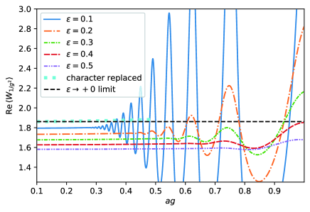
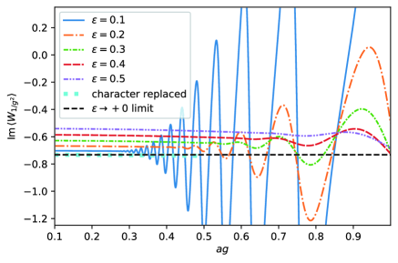
Figure 1: The expectation value of the Wilson loop $\langle W_{A}\rangle$ with the area $A=1/g^{2}$ evaluated with the analytic formula (3.9) for $SU(2)$. The values of $\varepsilon$ are varied to $\varepsilon=0.1,\cdots,0.5$. The cyan dotted line shows the $\varepsilon=0$ values with the modified Bessel function replaced by the asymptotic expansion dropping the unwanted part, which is drawn in the region where the asymptotic expansion gives a sufficient convergence up to the machine precision. The black dashed line shows the $a\rightarrow 0$, $\varepsilon\rightarrow+0$ value, eq. (3.10).

For completeness, we perform the $\varepsilon\rightarrow+0$ extrapolation of the $a\rightarrow 0$ limits. To obtain the $a\rightarrow 0$ values for each $\varepsilon$, we fit five points $a=0.1,0.15,\cdots,0.3$ with the linear function of $a^{2}$. The systematic error is calculated from the estimated variance of the fitting parameter. The obtained values for the $A=1$ case are shown in figure 2.

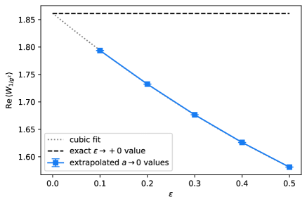
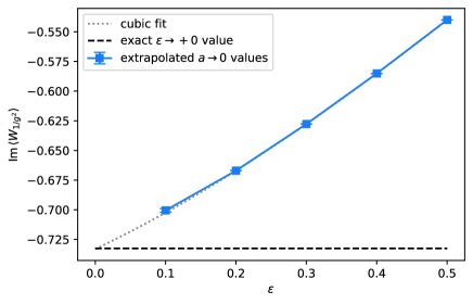
Figure 2: The extrapolated $a\rightarrow 0$ values of $\langle W_{1/g^{2}}\rangle$ with various $\varepsilon$ for $SU(2)$. The $a\rightarrow 0$ values are then fitted to obtain the final $\varepsilon\rightarrow+0$ result. The exact $\varepsilon\rightarrow+0$ value (3.10) is shown with the black dashed line for comparison.

We fit these values with a quadratic and cubic functions of $\varepsilon$ to give the final $\varepsilon\rightarrow+0$ value. We use the cubic result for the central value, and take the difference from the quadratic value as the estimate of the systematic error. The chi-squared for the cubic fits are $\chi^{2}/{\rm DOF}=3.3$ and $1.4$, respectively, for the real and imaginary parts. The obtained estimate $\lim_{a\rightarrow 0,\varepsilon\rightarrow+0}\langle W_{A=1}\rangle\approx 1.86146(93)-0.7331(36)i$ agrees with the analytical value $\lim_{a\rightarrow 0,\varepsilon\rightarrow+0}\langle W_{A=1}\rangle=1.8610-0.7325i$ within the estimated systematic error. To see how the finite $a$ or $\varepsilon$ effect depends on $A$, we also plot $\langle W_{A}\rangle$ with various $a$ for $\varepsilon=0.1$ (figure 3) and the $a\rightarrow 0$ values with various $\varepsilon$ (figure 4).

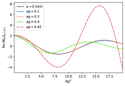
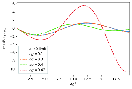
Figure 3: The area $A$ dependence of $\langle W_{A}\rangle$ evaluated with various $a$ keeping $\varepsilon=0.1$ fixed ($N_{c}=2$).

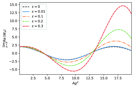
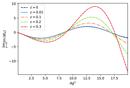
Figure 4: The area $A$ dependence of $\lim_{a\rightarrow 0}\langle W_{A}\rangle$ evaluated with various $\varepsilon$ ($N_{c}=2$).

We see that the effect of finite $a$ or $\varepsilon$ becomes larger as we increase $A$.

For $SU(3)$, we show in figure 5 the expectation value $\langle W_{A}\rangle$ with the area $A=1$ and in figure 6 the extrapolation of the $a\rightarrow 0$ values to the $\varepsilon\rightarrow+0$ limit.

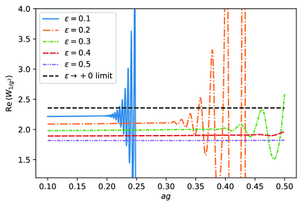
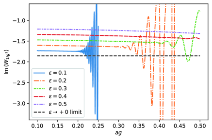
Figure 5: The expectation value of the Wilson loop $\langle W_{A}\rangle$ with the area $A=1/g^{2}$ evaluated with the analytic formula (3.9) for $SU(3)$. The values of $\varepsilon$ are varied to $\varepsilon=0.1,\cdots,0.5$. The plots are truncated before the curves become highly oscillatory. The black dashed line shows the $a\rightarrow 0$, $\varepsilon\rightarrow+0$ value, eq. (3.10).

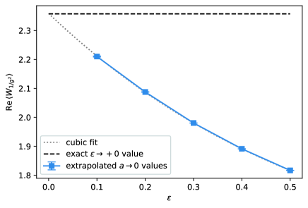
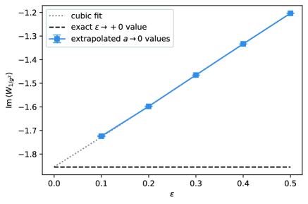
Figure 6: The extrapolated $a\rightarrow 0$ values of $\langle W_{1/g^{2}}\rangle$ with various $\varepsilon$ for $SU(3)$. The $a\rightarrow 0$ values are then fitted to obtain the final $\varepsilon\rightarrow+0$ result. The exact $\varepsilon\rightarrow+0$ value (3.10) is shown with the black dashed line for comparison.

The extrapolations are performed similarly to the $SU(2)$ case, where we replace the range of $a$ to $a=0.1,0.125,\cdots,0.2$. The obtained estimate $\lim_{a\rightarrow 0,\varepsilon\rightarrow+0}\langle W_{A=1}\rangle\approx 2.359(22)-1.854(19)i$ agrees with the analytical value $\lim_{a\rightarrow 0,\varepsilon\rightarrow+0}\langle W_{A=1}\rangle=2.358-1.855i$ within the error. The chi-squared for the cubic fits are $\chi^{2}/{\rm DOF}=3.3$ and $6.7$, respectively, for the real and imaginary parts. The above investigations show that the Wilson action with the $i\varepsilon$ correctly reproduces the appropriate continuum limit.

3.3 $i\varepsilon$ in the derivation of the path integral

In this subsection, we argue the reason why we need the $i\varepsilon$ for the Wilson action from the Hamiltonian formalism. For this, we use the $SU(2)$ Wilson action as an example, and follow the conventional Hamiltonian formalism of the Wilson action [46, 59]. To get rid of the complication related to the gauge symmetry, we take the temporal gauge, $U_{x,t}=1$. We keep the spatial lattice spacing $a$ finite in this subsection. Then, at time slice $t$, the degrees of freedom of the system are the spatial link variables $U_{\textbf{x},i}$. To describe fluctuations around $U_{\textbf{x},i}$, we introduce the local coordinates $\theta_{\textbf{x},i}^{a}$ by

$$e^{i\theta_{\textbf{x},i}^{a}T^{a}}U_{\textbf{x},i}.$$ (3.13)

In particular, we can track the infinitesimal time evolution in terms of $\theta_{\textbf{x},i}^{a}$. With the conjugate momentum:

$$p_{\textbf{x},i}^{a}\equiv\frac{a}{g^{2}}\dot{\theta}_{\textbf{x},i}^{a},$$ (3.14)

we can write down the Hamiltonian [46]:

$$H\equiv\frac{g^{2}}{2a}\sum_{\textbf{x},i}(p_{\textbf{x},i}^{a})^{2}+V(U),$$ (3.15)

where we defined the potential:

$$V(U)\equiv\frac{2N_{c}}{ag^{2}}\sum_{\textbf{x},i<j}\Big{(}1-\frac{1}{N_{c}}{\rm Re}\,{\rm tr}\,[U_{\textbf{x},i}U_{\textbf{x}+i,j}U_{\textbf{x}+j,i}^{\dagger}U_{\textbf{x},j}^{\dagger}]\Big{)}.$$ (3.16)

We now derive the amplitude in path integral form for the $SU(2)$ Wilson theory. The canonical operators $\hat{U}_{\textbf{x},i}$, $\hat{p}_{\textbf{x},i}^{a}$ satisfy the commutation relation:

$$[\hat{U}_{\textbf{x},i},\hat{p}_{\textbf{x},i}^{a}]=T^{a}\hat{U}_{\textbf{x},i}.$$ (3.17)

Configuration basis consists of the tensor product states:

$$|U\rangle\equiv\prod_{\textbf{x},i}|U_{\textbf{x},i}\rangle,$$ (3.18)

where

$$\hat{U}_{\textbf{x},i}|U_{\textbf{x},i}\rangle=U_{\textbf{x},i}|U_{\textbf{x},i}\rangle.$$ (3.19)

It is convenient to introduce another basis [60]:

$$|\{j_{\textbf{x},i},m_{\textbf{x},i},m_{\textbf{x},i}^{\prime}\}\rangle\equiv\prod_{\textbf{x},i}|j_{\textbf{x},i},m_{\textbf{x},i},m_{\textbf{x},i}^{\prime}\rangle,$$ (3.20)

where

$$\langle U_{\textbf{x},i}|j,m,m^{\prime}\rangle\equiv D_{m,m^{\prime}}^{j}(U_{\textbf{x},i})$$ (3.21)

with the matrix elements $D_{m,m^{\prime}}^{j}(U)$ of the $SU(2)$ matrix $U$ in the spin $j$ representation. From the Peter-Weyl theorem, the basis $|\{j_{\textbf{x},i},m_{\textbf{x},i},m_{\textbf{x},i}^{\prime}\}\rangle$ satisfies the completeness relation:

$$1=\sum_{\{j_{\textbf{x},i},m_{\textbf{x},i},m_{\textbf{x},i}^{\prime}\}}\Big{(}\prod_{\textbf{x},i}(2j_{\textbf{x},i}+1)\Big{)}|\{j_{\textbf{x},i},m_{\textbf{x},i},m_{\textbf{x},i}^{\prime}\}\rangle\langle\{j_{\textbf{x},i},m_{\textbf{x},i},m_{\textbf{x},i}^{\prime}\}|.$$ (3.22)

Furthermore, for finite $\eta_{\textbf{x},i}^{a}$,

$$\langle U_{\textbf{x},i}|e^{i\eta_{\textbf{x},i}^{a}\hat{p}_{\textbf{x},i}^{a}}|j,m,m^{\prime}\rangle =\big{(}Te^{i\int_{0}^{1}ds\,\eta_{\textbf{x},i}^{a}\mathcal{P}^{a}(s\eta_{\textbf{x},i})}\langle U_{\textbf{x},i}|\big{)}|j,m,m^{\prime}\rangle$$

$$=\big{[}Te^{i\int_{0}^{1}ds\,\eta_{\textbf{x},i}^{a}\mathcal{P}^{a}(s\eta_{\textbf{x},i})}D^{j}(U_{\textbf{x},i})\big{]}_{m,m^{\prime}},$$ (3.23)

where $T$ denotes the ordered product of the matrices and $\mathcal{P}^{a}(\theta)$ are the differential operators expressed in terms of the local coordinates on each link, $\theta^{a}$ [46, 59, 58, 60]. In particular, $-(\mathcal{P}^{a}(\theta))^{2}$ is the Laplacian on $S^{3}$ and $(\mathcal{P}^{a}(0))^{2}=(i^{-1}\partial_{\theta^{a}})^{2}$. Thus,

$$\langle U_{\textbf{x},i}|(\hat{p}_{\textbf{x},i}^{a})^{2}|j,m,m^{\prime}\rangle=[(\mathcal{P}^{a}(0))^{2}D^{j}(U_{\textbf{x},i})]_{m,m^{\prime}}=j(j+1)D^{j}_{m,m^{\prime}}(U_{\textbf{x},i}).$$ (3.24)

We now calculate the amplitude from the state $\psi_{i}$ to $\psi_{f}$:

$$A_{\psi_{f},\psi_{i}}(T)\equiv\langle\psi_{f}|e^{-i\hat{H}T}|\psi_{i}\rangle.$$ (3.25)

We discretize $T\equiv Na_{0}$ and ignore higher order terms of $a_{0}$. Note that

$$\langle U^{\prime}|e^{-ia_{0}\hat{H}}|U\rangle =\langle U^{\prime}|e^{-i\frac{a_{0}g^{2}}{2a}\sum_{\textbf{x},i}(\hat{p}_{{\textbf{x},i}}^{a})^{2}}e^{-ia_{0}V(\hat{U})}|U\rangle$$

$$=\prod_{\textbf{x},i}\Big{[}\sum_{j_{\textbf{x},i}}(2j_{\textbf{x},i}+1)\chi_{j_{\textbf{x},i}}(U^{\prime}_{{\textbf{x},i}}U_{{\textbf{x},i}}^{\dagger})e^{-i\frac{a_{0}g^{2}}{2a}j_{\textbf{x},i}(j_{\textbf{x},i}+1)}\Big{]}e^{-ia_{0}V(U)}.$$ (3.26)

By diagonalizing

$$U^{\prime}_{{\textbf{x},i}}U_{{\textbf{x},i}}^{\dagger}\sim{\rm diag}(e^{i\delta\phi_{\textbf{x},i}},e^{-i\delta\phi_{\textbf{x},i}})\quad\big{(}\delta\phi_{\textbf{x},i}\in[-\pi,\pi)\big{)},$$ (3.27)

we can write the expression in the bracket appearing in eq. (3.26) as (we drop the subscripts ${\textbf{x},i}$ temporarily for notational simplicity)

$$\sum_{j}(2j+1)\frac{\sin(2j+1)\delta\phi}{\sin\delta\phi}e^{-i\frac{a_{0}g^{2}}{2a}j(j+1)}$$

$$=-\frac{1}{2}\frac{1}{\sin\delta\phi}e^{i\frac{a_{0}g^{2}}{8a}}\frac{d}{d\delta\phi}\sum_{n\geq 1}\Big{[}e^{-i\frac{a_{0}g^{2}}{8a}n^{2}+in\delta\phi}+e^{-i\frac{a_{0}g^{2}}{8a}n^{2}-in\delta\phi}\Big{]}$$

$$=-\frac{1}{2}\frac{1}{\sin\delta\phi}e^{i\frac{a_{0}g^{2}}{8a}}\frac{d}{d\delta\phi}\vartheta\Big{(}\frac{\delta\phi}{2\pi},-\frac{a_{0}g^{2}}{8\pi a}\Big{)},$$ (3.28)

where we defined $n\equiv 2j+1$ in the second line. In order to further rewrite the expression, we introduce an infinitesimal imaginary part:

$$\vartheta\Big{(}\frac{\delta\phi}{2\pi},-\frac{a_{0}g^{2}}{8\pi a}\Big{)}\to\vartheta\Big{(}\frac{\delta\phi}{2\pi},-e^{-i\varepsilon}\frac{a_{0}g^{2}}{8\pi a}\Big{)}$$ (3.29)

The resulting function has a sharp peak around $\delta\phi=0$, and thus

$$-\frac{1}{2}\frac{1}{\sin\delta\phi}e^{i\frac{a_{0}g^{2}}{8a}}\frac{d}{d\delta\phi}\vartheta\Big{(}\frac{\delta\phi}{2\pi},-e^{-i\varepsilon}\frac{a_{0}g^{2}}{8\pi a}\Big{)}$$

$$\approx-\frac{1}{2}\frac{1}{\sin\delta\phi}e^{i\frac{a_{0}g^{2}}{8a}}\frac{d}{d\delta\phi}e^{i\pi/4}\sqrt{\frac{8\pi a}{-e^{-i\varepsilon}a_{0}g^{2}}}\exp\Big{[}ie^{i\varepsilon}\frac{2a}{a_{0}g^{2}}(\delta\phi)^{2}\Big{]}$$

$$={\rm const}\cdot\frac{\delta\phi}{\sin\delta\phi}\exp\Big{[}ie^{i\varepsilon}\frac{2a}{a_{0}g^{2}}(\delta\phi)^{2}\Big{]},$$ (3.30)

where in the second line we dropped the contributions with nontrivial winding that will be exponentially suppressed in the $a_{0}\rightarrow 0$ limit. Finite contribution comes from the fluctuations of order $\delta\phi=O(a_{0})$. With the similar argument as in eq. (2.29), we can rewrite eq. (3.30) up to an overall constant as

$${\rm const}\cdot\frac{\delta\phi}{\sin\delta\phi}\exp\Big{[}ie^{i\varepsilon}\frac{2a}{a_{0}g^{2}}(\delta\phi)^{2}\Big{]}={\rm const^{\prime}}\cdot\exp\Big{[}-ie^{i\varepsilon}\frac{2a}{a_{0}g^{2}}{\rm tr}\,[U^{\prime}U^{\dagger}]\Big{]}.$$ (3.31)

The amplitude is thus rewritten with the plaquette action in the desired path integral form with the $i\varepsilon$:

$$A_{n_{f},n_{i}}(T)\approx{\mathcal{N}}^{\prime}\lim_{\varepsilon\rightarrow+0}\int\Big{(}\prod_{\ell=0}^{N}dU_{\ell}\Big{)}\exp\Big{[}i\sum_{\ell=0}^{N-1}\Big{\{}-e^{i\varepsilon}\frac{2a}{a_{0}g^{2}}\sum_{\textbf{x},i}{\rm tr}[U_{\ell+1,\textbf{x},i}U_{\ell\textbf{x},i}^{\dagger}]$$

$$~{}~{}~{}~{}~{}~{}~{}~{}~{}~{}~{}~{}~{}~{}~{}~{}~{}~{}~{}~{}~{}~{}~{}~{}~{}~{}~{}~{}~{}~{}~{}~{}~{}+\frac{2a_{0}}{ag^{2}}\sum_{\textbf{x},i<j}{\rm tr}\,[U_{\ell,\textbf{x},i}U_{\ell,\textbf{x}+i,j}U_{\ell,\textbf{x}+j,i}^{\dagger}U_{\ell,\textbf{x},j}^{\dagger}]\Big{\}}\Big{]}\psi_{f}^{*}(U_{N})\psi_{i}(U_{0}),$$ (3.32)

where ${\mathcal{N}}^{\prime}$ is a normalization constant.

Despite the complications related to the field theory, the basic structure is the same as the quantum mechanical model in section 2. The Wilson action is only guaranteed to reproduce the continuum action for smooth fields, and we need to suppress the contributions from singular paths in advance with the $i\varepsilon$. The $i\varepsilon$ should thus be regarded as a part of the definition of the real-time path integral when using the Wilson action.

Note also that, since we only have considered the formal $a_{0}\rightarrow 0$ limit, the $i\varepsilon$ in the spatial plaquettes have not appeared in the discussion. In fact, in this treatment, the characters for the spatial plaquettes can be expressed in terms of the modified Bessel function of the form $I_{n}(2ia_{0}/(ag^{2}))$ [see eq. (3.5)], for which we can apply the expansion of $I_{n}(z)$ around zero:

$$I_{n}(z)=\Big{(}\frac{z}{2}\Big{)}^{n}\sum_{k\geq 0}\frac{(z/2)^{2k}}{n!(n+k)!}.$$ (3.33)

The characters coming from the spatial plaquettes are thus analytic in the limit $a_{0}\rightarrow 0$ for a fixed $a$, giving no complication. The subtlety for the spatial plaquettes arises when we take the continuum limit taking $a_{0}\rightarrow 0$ and $a\rightarrow 0$ at the same time, making $g^{2}$ run according to the renormalization group equation. In the latter treatment, which is required in extracting the continuum physics, we need to incorporate $i\varepsilon$ also for the spatial plaquettes as argued in subsection 3.1.

4 Summary and outlook

In this paper, we discussed that the $i\varepsilon$ is an essential ingredient in defining the real-time path integral for the Wilson action, and showed how its necessity can be explained from the Hamiltonian formalism. In numerical calculations, one needs to take the $i\varepsilon$ into account both for the timelike and spacelike plaquettes, and this can be done by calculating the continuum limit with several $\varepsilon$ and taking the $\varepsilon\rightarrow+0$ limit, or rewriting the Boltzmann weight in terms of characters dropping the unwanted part of the asymptotic expansion of modified Bessel function for the character coefficients. We in particular demonstrated that, with the $i\varepsilon$, the Wilson action gives the correct continuum limit using the two-dimensional theory as an example. We believe that this clarification of the subtlety helps us investigate more involved cases such as full quantum chromodynamics.

As we commented in section 3.2, we need to choose $\varepsilon$ large enough for a given lattice spacing to avoid the oscillation coming from the unwanted part of the asymptotic expansion. For the studied range of the lattice spacing, this is satisfied numerically in two-dimension at $\beta_{t}\sin\varepsilon\gtrsim 4.5$ for $SU(2)$ and $\beta_{t}\sin\varepsilon\gtrsim 15$ for $SU(3)$. Since the characters are expressed with $\beta_{r}$ in eq. (3.5), these values should give a rough estimate of the required $\varepsilon$ also in higher dimensions. The rather large bounds are, however, unpleasant for the four-dimensional application because of the existence of the critical slowing down at large $\beta_{r}$. A similar situation occurs for the action expressed with the characters in which the modified Bessel function is replaced by its asymptotic expansion dropping the unwanted part. This is because the asymptotic expansion itself is divergent, and thus we need to choose the order to truncate the expansion. For large enough $\beta_{r}$, the summand becomes smaller than the machine precision at some order, and thus we can truncate the expansion there. However, comparably large $\beta_{r}$ is required for such convergence especially in the $SU(3)$ case. Therefore, though our method gives a way to obtain the appropriate continuum prediction, it is desirable to circumvent the critical slowing down (see, e.g., [61, 62, 63, 64, 65, 66, 67, 68, 69, 70, 71, 72]) or develop an action that is convergent at small $\beta_{r}$ by, e.g., the contour deformation [30]. Studies along these lines are in progress and will be reported elsewhere.

References

- [1] R. P. Feynman, “Space-time approach to nonrelativistic quantum mechanics,” Rev. Mod. Phys. 20, 367-387 (1948).
- [2] E. Witten, “Analytic Continuation Of Chern-Simons Theory,” AMS/IP Stud. Adv. Math. 50, 347-446 (2011) [arXiv:1001.2933 [hep-th]].
- [3] Y. Tanizaki and T. Koike, “Real-time Feynman path integral with Picard–Lefschetz theory and its applications to quantum tunneling,” Annals Phys. 351, 250-274 (2014) [arXiv:1406.2386 [math-ph]].
- [4] N. Turok, “On Quantum Tunneling in Real Time,” New J. Phys. 16, 063006 (2014) [arXiv:1312.1772 [quant-ph]].
- [5] J. Berges, S. Borsanyi, D. Sexty and I. O. Stamatescu, “Lattice simulations of real-time quantum fields,” Phys. Rev. D 75, 045007 (2007) [arXiv:hep-lat/0609058 [hep-lat]].
- [6] J. Berges and D. Sexty, “Real-time gauge theory simulations from stochastic quantization with optimized updating,” Nucl. Phys. B 799, 306-329 (2008) [arXiv:0708.0779 [hep-lat]].
- [7] A. Alexandru, G. Basar, P. F. Bedaque, S. Vartak and N. C. Warrington, “Monte Carlo Study of Real Time Dynamics on the Lattice,” Phys. Rev. Lett. 117, no.8, 081602 (2016) [arXiv:1605.08040 [hep-lat]].
- [8] A. Alexandru, G. Basar, P. F. Bedaque and G. W. Ridgway, “Schwinger-Keldysh formalism on the lattice: A faster algorithm and its application to field theory,” Phys. Rev. D 95, no.11, 114501 (2017) [arXiv:1704.06404 [hep-lat]].
- [9] Z. G. Mou, P. M. Saffin, A. Tranberg and S. Woodward, “Real-time quantum dynamics, path integrals and the method of thimbles,” JHEP 06, 094 (2019) [arXiv:1902.09147 [hep-lat]].
- [10] S. Takeda, “A novel method to evaluate real-time path integral for scalar theory,” [arXiv:2108.10017 [hep-lat]].
- [11] G. Fujisawa, J. Nishimura, K. Sakai and A. Yosprakob, “Backpropagating Hybrid Monte Carlo algorithm for fast Lefschetz thimble calculations,” [arXiv:2112.10519 [hep-lat]].
- [12] S. K. Asante, B. Dittrich and J. Padua-Argüelles, “Complex actions and causality violations: Applications to Lorentzian quantum cosmology,” [arXiv:2112.15387 [gr-qc]].
- [13] G. Parisi, “On complex probabilities,” Phys. Lett. B 131, 393 (1983).
- [14] J.R. Klauder, “Coherent State Langevin Equations for Canonical Quantum Systems With Applications to the Quantized Hall Effect,” Phys. Rev. A 29, 2036 (1984).
- [15] G. Aarts, F. A. James, E. Seiler and I. O. Stamatescu, “Adaptive stepsize and instabilities in complex Langevin dynamics,” Phys. Lett. B 687, 154-159 (2010) [arXiv:0912.0617 [hep-lat]].
- [16] J. Nishimura and S. Shimasaki, “New Insights into the Problem with a Singular Drift Term in the Complex Langevin Method,” Phys. Rev. D 92, no.1, 011501 (2015) [arXiv:1504.08359 [hep-lat]].
- [17] M. Cristoforetti, F. Di Renzo and L. Scorzato, “New approach to the sign problem in quantum field theories: High density QCD on a Lefschetz thimble,” Phys. Rev. D 86, 074506 (2012) [arXiv:1205.3996 [hep-lat]].
- [18] M. Cristoforetti, F. Di Renzo, A. Mukherjee and L. Scorzato, “Monte Carlo simulations on the Lefschetz thimble: Taming the sign problem,” Phys. Rev. D 88, no. 5, 051501(R) (2013) [arXiv:1303.7204 [hep-lat]].
- [19] H. Fujii, D. Honda, M. Kato, Y. Kikukawa, S. Komatsu and T. Sano, “Hybrid Monte Carlo on Lefschetz thimbles - A study of the residual sign problem,” JHEP 1310, 147 (2013) [arXiv:1309.4371 [hep-lat]].
- [20] A. Alexandru, G. Başar, P. F. Bedaque, G. W. Ridgway and N. C. Warrington, “Sign problem and Monte Carlo calculations beyond Lefschetz thimbles,” JHEP 1605, 053 (2016) [arXiv:1512.08764 [hep-lat]].
- [21] M. Fukuma and N. Umeda, “Parallel tempering algorithm for integration over Lefschetz thimbles,” PTEP 2017, no. 7, 073B01 (2017) [arXiv:1703.00861 [hep-lat]].
- [22] A. Alexandru, G. Başar, P. F. Bedaque and N. C. Warrington, “Tempered transitions between thimbles,” Phys. Rev. D 96, no. 3, 034513 (2017) [arXiv:1703.02414 [hep-lat]].
- [23] M. Fukuma, N. Matsumoto and N. Umeda, “Applying the tempered Lefschetz thimble method to the Hubbard model away from half filling,” Phys. Rev. D 100, no. 11, 114510 (2019) [arXiv:1906.04243 [cond-mat.str-el]].
- [24] M. Fukuma, N. Matsumoto and N. Umeda, “Implementation of the HMC algorithm on the tempered Lefschetz thimble method,” [arXiv:1912.13303 [hep-lat]].
- [25] M. Fukuma and N. Matsumoto, “Worldvolume approach to the tempered Lefschetz thimble method,” PTEP 2021, no.2, 023B08 (2021) [arXiv:2012.08468 [hep-lat]].
- [26] M. Fukuma, N. Matsumoto and Y. Namekawa, “Statistical analysis method for the worldvolume hybrid Monte Carlo algorithm,” PTEP 2021, no.12, 123B02 (2021) [arXiv:2107.06858 [hep-lat]].
- [27] Y. Mori, K. Kashiwa and A. Ohnishi, “Toward solving the sign problem with path optimization method,” Phys. Rev. D 96, no.11, 111501 (2017) [arXiv:1705.05605 [hep-lat]].
- [28] Y. Mori, K. Kashiwa and A. Ohnishi, “Application of a neural network to the sign problem via the path optimization method,” PTEP 2018, no.2, 023B04 (2018) [arXiv:1709.03208 [hep-lat]].
- [29] A. Alexandru, P. F. Bedaque, H. Lamm and S. Lawrence, “Finite-Density Monte Carlo Calculations on Sign-Optimized Manifolds,” Phys. Rev. D 97, no.9, 094510 (2018) [arXiv:1804.00697 [hep-lat]].
- [30] G. Kanwar and M. L. Wagman, “Real-time lattice gauge theory actions: Unitarity, convergence, and path integral contour deformations,” Phys. Rev. D 104, no.1, 014513 (2021) [arXiv:2103.02602 [hep-lat]].
- [31] H. Niggemann, A. Klumper and J. Zittartz, “Quantum phase transition in spin 3/2 systems on the hexagonal lattice: Optimum ground state approach,” Z. Phys. B 104, 103-110 (1997) [arXiv:cond-mat/9702178 [cond-mat]].
- [32] F. Verstraete and J. I. Cirac, “Renormalization algorithms for quantum-many body systems in two and higher dimensions,” [arXiv:cond-mat/0407066 [cond-mat]].
- [33] M. Levin and C. P. Nave, “Tensor renormalization group approach to 2D classical lattice models,” Phys. Rev. Lett. 99, no.12, 120601 (2007) [arXiv:cond-mat/0611687 [cond-mat.stat-mech]].
- [34] Z. Y. Xie, H. C. Jiang, Q. N. Chen, Z. Y. Weng and T. Xiang, “Second Renormalization of Tensor-Network States,” Phys. Rev. Lett. 103, 160601 (2009) [arXiv:0809.0182 [cond-mat.str-el]].
- [35] Z. C. Gu, F. Verstraete and X. G. Wen, “Grassmann tensor network states and its renormalization for strongly correlated fermionic and bosonic states,” [arXiv:1004.2563 [cond-mat.str-el]].
- [36] Z. Y. Xie, and J. Chen, and M. P. Qin,and J. W. Zhu, and L. P. Yang, and T. Xiang, “Coarse-graining renormalization by higher-order singular value decomposition,” Phys. Rev. B 86, no.4, 045139 (2012) [arXiv:1201.1144 [cond-mat.stat-mech]].
- [37] D. Adachi, T. Okubo and S. Todo, “Anisotropic Tensor Renormalization Group,” Phys. Rev. B 102, no.5, 054432 (2020) [arXiv:1906.02007 [cond-mat.stat-mech]].
- [38] D. Kadoh and K. Nakayama, “Renormalization group on a triad network,” [arXiv:1912.02414 [hep-lat]].
- [39] M. Fukuma, D. Kadoh and N. Matsumoto, “Tensor network approach to two-dimensional Yang–Mills theories,” PTEP 2021, no.12, 123B03 (2021) [arXiv:2107.14149 [hep-lat]].
- [40] M. Hirasawa, A. Matsumoto, J. Nishimura and A. Yosprakob, “Tensor renormalization group and the volume independence in 2D U(N) and SU(N) gauge theories,” JHEP 12, 011 (2021) [arXiv:2110.05800 [hep-lat]].
- [41] H. Hoshina, H. Fujii and Y. Kikukawa, “Schwinger-Keldysh formalism for Lattice Gauge Theories,” PoS LATTICE2019, 190 (2020).
- [42] A. H. Fatollahi, “Worldline as a Spin Chain,” Eur. Phys. J. C 77, no.3, 159 (2017) [arXiv:1611.08009 [hep-th]].
- [43] W. Langguth and A. Inomata, “Remarks on the Hamiltonian path integral in polar coordinates,” J. Math. Phys. 20, 499-504 (1979).
- [44] M. Böhm and G. Junker, “Path integration over compact and noncompact rotation groups,” J. Math. Phys. 28, 1978-1994 (1987).
- [45] G. C. Wick, “Properties of Bethe-Salpeter Wave Functions,” Phys. Rev. 96, 1124-1134 (1954).
- [46] J. B. Kogut and L. Susskind, “Hamiltonian Formulation of Wilson’s Lattice Gauge Theories,” Phys. Rev. D 11, 395-408 (1975).
- [47] D. Judge, J.T. Lewis, “On the commutator ”, Physics Letters, Volume 5, Issue 3, Page 190 (1963).
- [48] L. Susskind and J. Glogower, “Quantum mechanical phase and time operator,” Physics Physique Fizika 1, no.1, 49-61 (1964).
- [49] P. Carruthers and M. M. Nieto, “Phase and angle variables in quantum mechanics,” Rev. Mod. Phys. 40, 411-440 (1968).
- [50] Akira Inomata, Vijay A. Singh, “Path integrals and constraints: Particle in a box,” Physics Letters A, Volume 80, Issues 2, 105-108 (1980).
- [51] Y. Ohnuki and S. Kitakado, “Quantum mechanics on a closed loop,” Mod. Phys. Lett. A 9, 143-150 (1994).
- [52] S. Tanimura, “Gauge field, parity and uncertainty relation of quantum mechanics on S(1),” Prog. Theor. Phys. 90, 271-292 (1993) [arXiv:hep-th/9306098 [hep-th]].
- [53] K. Fukushima, T. Shimazaki and Y. Tanizaki, “Exploring the -vacuum structure in the functional renormalization group approach,” JHEP 04, 040 (2022) [arXiv:2202.00375 [hep-th]].
- [54] K. G. Wilson, “Confinement of Quarks,” Phys. Rev. D 10 (1974), 2445-2459.
- [55] R. Brower, P. Rossi and C. I. Tan, “The External Field Problem for QCD,” Nucl. Phys. B 190, 699-718 (1981).
- [56] J. M. Drouffe and J. B. Zuber, “Strong Coupling and Mean Field Methods in Lattice Gauge Theories,” Phys. Rept. 102, 1 (1983).
- [57] D. J. Gross and E. Witten, “Possible Third Order Phase Transition in the Large N Lattice Gauge Theory,” Phys. Rev. D 21, 446-453 (1980).
- [58] P. Menotti and E. Onofri, “The Action of SU() Lattice Gauge Theory in Terms of the Heat Kernel on the Group Manifold,” Nucl. Phys. B 190, 288-300 (1981).
- [59] M. Creutz, “Gauge Fixing, the Transfer Matrix, and Confinement on a Lattice,” Phys. Rev. D 15, 1128 (1977).
- [60] S. A. Chin, O. S. Van Roosmalen, E. A. Umland and S. E. Koonin, “EXACT GROUND STATE PROPERTIES OF THE SU(2) HAMILTONIAN LATTICE GAUGE THEORY,” Phys. Rev. D 31, 3201-3212 (1985).
- [61] G. Parisi, “PROLEGOMENA TO ANY FUTURE COMPUTER EVALUATION OF THE QCD MASS SPECTRUM,” Progress in Gauge Field Theory, edited by ’t Hooft et al. (Plenum, New York, 1984), p.351.
- [62] G. G. Batrouni, G. R. Katz, A. S. Kronfeld, G. P. Lepage, B. Svetitsky and K. G. Wilson, “Langevin Simulations of Lattice Field Theories,” Phys. Rev. D 32, 2736 (1985).
- [63] C. T. H. Davies, G. G. Batrouni, G. R. Katz, A. S. Kronfeld, G. P. Lepage, K. G. Wilson, P. Rossi and B. Svetitsky, “Fourier Acceleration in Lattice Gauge Theories. 1. Landau Gauge Fixing,” Phys. Rev. D 37, 1581 (1988).
- [64] G. Katz, G. Batrouni, C. Davies, A. S. Kronfeld, P. Lepage, P. Rossi, B. Svetitsky and K. Wilson, “Fourier Acceleration. 2. Matrix Inversion and the Quark Propagator,” Phys. Rev. D 37, 1589 (1988).
- [65] C. T. H. Davies, G. G. Batrouni, G. R. Katz, A. S. Kronfeld, G. P. Lepage, P. Rossi, B. Svetitsky and K. G. Wilson, “Fourier Acceleration in Lattice Gauge Theories. 3. Updating Field Configurations,” Phys. Rev. D 41, 1953 (1990).
- [66] M. Luscher, “Trivializing maps, the Wilson flow and the HMC algorithm,” Commun. Math. Phys. 293, 899-919 (2010) [arXiv:0907.5491 [hep-lat]].
- [67] M. Luscher and S. Schaefer, “Lattice QCD without topology barriers,” JHEP 07, 036 (2011) [arXiv:1105.4749 [hep-lat]].
- [68] M. S. Albergo, G. Kanwar and P. E. Shanahan, “Flow-based generative models for Markov chain Monte Carlo in lattice field theory,” Phys. Rev. D 100, no.3, 034515 (2019) [arXiv:1904.12072 [hep-lat]].
- [69] S. Foreman, X. Y. Jin and J. C. Osborn, “Deep Learning Hamiltonian Monte Carlo,” [arXiv:2105.03418 [hep-lat]].
- [70] D. Albandea, P. Hernández, A. Ramos and F. Romero-López, “Topological sampling through windings,” Eur. Phys. J. C 81, no.10, 873 (2021) [arXiv:2106.14234 [hep-lat]].
- [71] S. Foreman, T. Izubuchi, L. Jin, X. Y. Jin, J. C. Osborn and A. Tomiya, “HMC with Normalizing Flows,” [arXiv:2112.01586 [cs.LG]].
- [72] T. Nguyen, P. Boyle, N. Christ, Y. C. Jang and C. Jung, “Riemannian manifold hybrid Monte Carlo in lattice QCD,” [arXiv:2112.04556 [hep-lat]].