Progressive Purification for Instance-Dependent Partial Label Learning

Abstract

Partial label learning (PLL) aims to train multi-class classifiers from the examples each annotated with a set of candidate labels where a fixed but unknown candidate label is correct. In the last few years, the instance-independent generation process of candidate labels has been extensively studied, on the basis of which many theoretical advances have been made in PLL. Nevertheless, the candidate labels are always instance-dependent in practice and there is no theoretical guarantee that the model trained on the instance-dependent PLL examples can converge to an ideal one. In this paper, a theoretically grounded and practically effective approach named Pop, i.e. PrOgressive Purification for instance-dependent partial label learning, is proposed. Specifically, Pop updates the learning model and purifies each candidate label set progressively in every epoch. Theoretically, we prove that Pop enlarges the region appropriately fast where the model is reliable, and eventually approximates the Bayes optimal classifier with mild assumptions. Technically, Pop is flexible with arbitrary PLL losses and could improve the performance of the previous PLL losses in the instance-dependent case. Experiments on the benchmark datasets and the real-world datasets validate the effectiveness of the proposed method.

1 Introduction

The difficulty of collecting large scale datasets with high-quality annotations for training classifiers induces weakly supervised learning, a typical example among which is partial label learning (PLL) (Nguyen & Caruana, 2008; Cour et al., 2011; Zhang et al., 2017b; Yao et al., 2020b; Lv et al., 2020; Feng et al., 2020b; Wen et al., 2021). PLL deals with the problem where each training example is associated with a set of candidate labels, among which only one label is valid. This paradigm naturally arises in various real-world applications, such as web mining (Luo & Orabona, 2010), multimedia content analysis (Zeng et al., 2013), ecoinformatics (Tang & Zhang, 2017), etc.

A large number of deep PLL algorithms have recently emerged that aimed to design regularizers (Yao et al., 2020a, b; Lyu et al., 2022) or network architectures (Wang et al., 2022) for PLL data. Further, there are some PLL works that provided theoretical guarantees while making their methods compatible with deep networks (Lv et al., 2020; Feng et al., 2020b; Wen et al., 2021; Wu & Sugiyama, 2021). These existing works have focused on the instance-independent setting where the generation process of candidate labels is homogeneous across training examples. With an explicit formulation of the generation process, the asymptotical consistency (Mohri et al., 2018) of the methods, i.e., the classifier learned from partially labeled examples could approximate the Bayes optimal classifier, can be analyzed.

Previous works have extensively studied instance-independent PLL and many theoretical advances have been made in this setting. However, the candidate labels are always instance-dependent (feature-dependent) in practice as the incorrect labels related to the feature are more likely to be picked as candidate label set for each instance. Therefore, instance-dependent (ID) candidate labels (Xu et al., 2021b) should be quite realistic and could describe the ambiguous labeling information for the instance which is difficult to be annotated with an exact true label in PLL. By adopting the latent label distributions, recent work (Xu et al., 2021b) has empirically validated that the classifier trained on instance-dependent PLL examples could achieve good performance. Nevertheless, there is no theoretical guarantee that the model trained on the instance-dependent PLL examples can converge to an ideal one.

In this paper, we propose a theoretically grounded method named Pop, i.e. PrOgressive Purification for instance-dependent partial label learning. Specifically, the observed candidate labels are utilized to train a randomly initialized classifier (deep network) for several epochs, and then the classifier is updated with purified candidate label set for the remaining epochs. In each epoch, each candidate label set is purified according to the pure level set with the classifier for candidate labels and we prove that Pop can be guaranteed to enlarge the region where the model is reliable by a promising rate. As a consequence, the false candidate labels are gradually moved out and the classification performance of the classifier is improved. We justify Pop and outline the main contributions below:

• We propose a novel approach named Pop for the instance-dependent PLL problem, which purifies the candidate label sets and refines the classifier iteratively. Extensive experiments validate the effectiveness of Pop.

• We prove that Pop can be guaranteed to enlarge the region where the model is reliable by a promising rate, and eventually approximates the Bayes optimal classifier with mild assumptions. To the best of our knowledge, this is the first theoretically guaranteed approach for instance-dependent PLL.

• Pop is flexible with respect to losses, so that the losses designed for the instance-independent PLL problems can be embedded directly. We empirically show that such embedding allows advanced PLL losses can be applied to the instance-dependent PLL problem and achieve state-of-the-art learning performance.

2 Related Work

In this section, we briefly go through the seminal works in PLL, focusing on the theoretical works and discussing the underlying assumptions behind them.

There have been substantial traditional PLL algorithms from the pioneering work (Jin & Ghahramani, 2003). From a practical standpoint, they have been studied along two different research routes: the identification-based strategy and the average-based strategy. The identification-based strategy purifies each partial label and extracts the true label heuristically in the training phase, so as to identify the true labels (Chen et al., 2014; Zhang et al., 2016; Tang & Zhang, 2017; Feng & An, 2019; Xu et al., 2019). On the contrary, the average-based strategy treats all candidates equally (Hüllermeier & Beringer, 2006; Cour et al., 2011; Zhang & Yu, 2015). On the theoretical side, Liu and Dietterich (Liu & Dietterich, 2012) analyzed the learnability of PLL by making a small ambiguity degree condition assumption, which ensures classification errors on any instance have a probability of being detected. And Cour et al. (Cour et al., 2011) proposed a consistent approach under the small ambiguity degree condition and a dominance assumption on data distribution. Liu and Dietterich (Liu & Dietterich, 2012) proposed a Logistic Stick-Breaking Conditional Multinomial Model to portray the mapping between instances and true labels while assuming the generation of the partial label is independent of the instance itself. The label distribution is adopted to disambiguate the candidate labels (Xu et al., 2019) via recovering the latent label distribution in the label enhancement process (Xu et al., 2021a, 2022, 2023). It should be noted that the vast majority of traditional PLL works have only empirically verified the performance of algorithms on small data sets, without formalizing the statistical model for the PLL problem, and therefore even less so for theoretical analysis of when and why the algorithms work.

In recent years, deep learning has been applied to PLL and has greatly advanced the practical application of PLL. Yao et al. (Yao et al., 2020a, b) and Lv et al. (Lv et al., 2020) proposed learning objectives that are compatible with stochastic optimization and thus can be implemented by deep networks. Soon Feng et al. (Feng et al., 2020b) formalized the first generation process for PLL. They assumed that given the latent true label, the probability of all incorrect labels being added into the candidate label set is uniform and independent of the instance. Thanks to the uniform generation process, they proposed two provably consistent algorithms. Wen et al. (Wen et al., 2021) extended the uniform one to the class-dependent case, but still keep the instance-independent assumption unchanged. In addition, a new paradigm called complementary label learning (Ishida et al., 2017; Yu et al., 2018; Ishida et al., 2019; Feng et al., 2020a) has been proposed that learns from instances equipped with a complementary label. A complementary label specifies the classes to which the instance does not belong, so it can be considered to be an inverted PLL problem. However, all of them made the instance-independent assumption for analyzing the statistic consistency. Wu and Sugiyama (Wu & Sugiyama, 2021) proposed a framework that unifies the formalization of multiple generation processes under the instance-independent assumption. Wang et al. (Wang et al., 2022) proposed a data-augmentation-based framework to disambiguate partial labels with contrastive learning. Zhang et al. (Zhang et al., 2021a) exploited the class activation value to identify the true label in candidate label sets.

Very recently, some researchers are beginning to notice a more general setting— instance-independent (ID) PLL. Learning with the ID partial labels is challenging, and all instance-independent approaches cannot handle the ID PLL problem directly. Specifically, the theoretical approaches mentioned above utilize mainly the loss correction technique, which corrects the prediction or the loss of the classifier using a prior or estimated knowledge of data generation processes, i.e., a set of parameters controlling the probability of generating incorrect candidate labels, or it is often called transition matrix (Patrini et al., 2017). The transition matrix can be characterized fixedly in the instance-independent setting since it does not need to include instance-level information, a condition that does not hold in ID PLL. Furthermore, it is ill-posed to estimate the transition matrix by only exploiting partially labeled data, i.e., the transition matrix is unidentifiable (Xia et al., 2020). Therefore, some new methods should be proposed to tackle this issue. Xu et al. (Xu et al., 2021b) introduced a solution that infers the latent label posterior via variational inference methods (Blei et al., 2017), nevertheless, its effectiveness would be hardly guaranteed. In this paper, we propose Pop for the ID PLL problem and theoretically prove that the learned classifier approximates well to the Bayes optimal.

3 Proposed Method

3.1 Preliminaries

First of all, we briefly introduce some necessary notations. Consider a multi-class classification problem of $c$ classes. Let $\mathcal{X}=\mathbb{R}^{q}$ be the $q$-dimensional instance space and $\mathcal{Y}=\{1,2,\ldots,c\}$ be the label space with $c$ class labels. In supervised learning, let $p(\bm{x},y)$ be the underlying “clean” distribution generating $(\bm{x},y^{\bm{x}})\in\mathcal{X}\times\mathcal{Y}$ from which $n$ i.i.d. samples $\{(\bm{x}_{i},y^{\bm{x}_{i}})\}^{n}_{i=1}$ are drawn.

In PLL, there is a candidate label space $\mathcal{S}:=\{S|S\subseteq\mathcal{Y},S\neq\emptyset\}$ and the PLL training set $\mathcal{D}=\{(\bm{x}_{i},S_{i})|1\leq i\leq n\}$ is sampled independently and identically from a “corrupted” density $\tilde{p}(\bm{x},S)$ over $\mathcal{X}\times\mathcal{S}$. It is generally assumed that $p(\bm{x},y)$ and $p(\bm{x},S)$ have the same marginal distribution of instances $p(\bm{x})$. Then the generation process of partial labels can thus be formalized as $p(S|\bm{x})=\sum_{y}p(S|\bm{x},y)p(y|\bm{x})$. We define the probability that, given the instance $\bm{x}$ and its class label $y^{\bm{x}}$, $j$-label being included in its partial label as the flipping probability:

$$\xi^{j}(\bm{x})=p(j\in S|\bm{x},y^{\bm{x}}),\ \forall j\in\mathcal{Y},$$

The key definition in PLL is that the latent true label of an instance is always one of its candidate label, i.e., $\xi^{y^{\bm{x}}}(\bm{x})=1$.

We consider use deep models by the aid of an inverse link function (Reidand & Williamson, 2010) $\bm{\phi}:\mathbb{R}^{c}\rightarrow\Delta^{c-1}$ where $\Delta^{c-1}$ denotes the $c$-dimensional simplex, for example, the softmax, as learning model in this paper. Then the goal of supervised multi-class classification and PLL is the same: a scoring function $f:\mathcal{X}\mapsto\Delta^{c-1}$ that can make correct predictions on unseen inputs. Typically, the classifier takes the form:

$$h(\bm{x})=\arg\max_{j\in\mathcal{Y}}f_{j}(\bm{x}).$$

The Bayes optimal classifier $h^{\star}$ (learned using supervised data) is the one that minimizes the risk w.r.t the 0-1 loss (or some classification-calibrated loss (Bartlett et al., 2006)), i.e.,

$$h^{\star}=\arg\min_{h}\mathcal{R}_{01}=\arg\min_{h}\mathbb{E}_{(\bm{X},Y)\sim p(\bm{x},y)}\big{[}\mathbf{1}_{\{h(\bm{X})\neq Y\}}\big{]}.$$

For strictly proper losses (Gneiting & Raftery, 2007), the scoring function $f^{*}$ recovers the class-posterior probabilities, i.e., $f^{\star}(\bm{x})=p(y|\bm{x}),\forall\bm{x}\in\mathcal{X}$. When the supervision information available is partial label, the PLL risk under $\tilde{p}(\bm{x},S)$ w.r.t. a suitable PLL loss $\mathcal{L}:\mathbb{R}^{k}\times\mathcal{S}\rightarrow\mathbb{R}^{+}$ is defined as

$$\tilde{\mathcal{R}}=\mathbb{E}_{(\bm{X},S)\sim\tilde{p}(\bm{x},S)}\big{[}\mathcal{L}(h(\bm{X}),S)\big{]}.$$

Minimizing $\tilde{\mathcal{R}}$ induces the classifier and it is desirable that the minimizer approach $h^{\star}$. In addition, let $o=\arg\max_{j\neq y^{\bm{x}}}p(y=j|\bm{x})$ be the class label with the second highest posterior possibility among all labels.

3.2 Overview

In the latter part of this section, we will introduce a concept pure level set as the region where the model is reliable. We prove that given a tiny reliable region, one could progressively enlarge this region and improves the model with a sufficient rate by disambiguating the partial labels. Motivated by the theoretical results, we propose an approach Pop that works by progressively purifying the partial labels to move out the false candidate labels, and eventually the learned classifier could approximate the Bayes optimal classifier.

Pop employs the observed partial labels to pre-train a randomly initialized classifier for several epochs, and then updates both partial labels and the classifier for the remaining epochs. We start with a warm-up period, in which we train the predictive model with a well-defined PLL loss (Lv et al., 2020). This allows us to attain a reasonable predictive model before it starts fitting incorrect labels (Zhang et al., 2017a). After the warm-up period, we iteratively purify each partial label by moving out the candidate labels for which the current classifier has high confidence of being incorrect, and subsequently we train the classifier with the purified partial labels in the next epoch. After the model has been fully trained, the predictive model can perform prediction for unseen instances.

3.3 The Pop Approach

We assume that the hypothesis class $\mathcal{H}$ is sufficiently complex (and deep networks could meet this condition), such that the approximation error equals zero, i.e., $\arg\min_{h}\mathcal{R}=\arg\min_{h\in\mathcal{H}}\mathcal{R}$ and we have enough training data i.e., $n\rightarrow\infty$. The classifier is able to at least approximate the Bayes optimal classifier $h^{\star}$ and the gap between the learned $f(\bm{x})$ and the the scoring function $f^{\star}(\bm{x})$ corresponding to $h^{\star}$ is determined by the inconsistency between incorrect candidate labels and output of the Bayes optimal classifier.

For two instance $\bm{x}$ and $\bm{z}$ that satisfy $p(y^{\bm{z}}|\bm{z})-p(o|\bm{z})\geq p(y^{\bm{x}}|\bm{x})-p(o|\bm{x})$, i.e., the margin between the posterior of ground-truth label $p(y^{\bm{z}}|\bm{z})$ and the second highest posterior possibility $p(o|\bm{z})$ is larger than that in point $\bm{x}$, the indicator function $\big{[}\mathbf{1}_{\{{{j\neq h^{\star}(\bm{z})}}\}}\Big{|}{}p(y^{\bm{z}}|\bm{z})-p(o|\bm{z})\geq p(y^{\bm{x}}|\bm{x})-p(o|\bm{x}),~{}j\in S_{\bm{z}}\big{]}$ equals 1 if the candidate label $j$ of $\bm{z}$ is inconsistent with the output of the optimal Bayes classifier $h^{\star}(\bm{z})$. Then, the gap between $f_{j}(\bm{x})$ and $f^{\star}_{j}(\bm{x})$ , i.e., the approximation error of the classifier, could be controlled by the inconsistency between the incorrect candidate labels and the output of the Bayes optimal classifier $h^{\star}$ for all the instances $\bm{z}$. Therefore, we assume that there exist constants $\alpha$, $\epsilon<1$, such that for $f(\bm{x})$,

$$\begin{split}|f^{j}(\bm{x})-p(y=j|\bm{x})|\leq\alpha\mathbb{E}_{(\bm{z},S)\sim\tilde{p}(\bm{z},S)}\bigg{[}\mathbf{1}_{\{j\neq y^{\bm{z}}\}}\Big{|}\\ p(y^{\bm{z}}|\bm{z})-p(o|\bm{z})\geq p(y^{\bm{x}}|\bm{x})-p(o|\bm{x})\bigg{]}+\frac{\epsilon}{6}\end{split}$$ (1)

where the scoring function $f^{*}$ corresponding to $h^{*}$ on strictly proper losses (Gneiting & Raftery, 2007) recovers the class-posterior probabilities, i.e., $f^{\star}_{j}(\bm{x})=p(y=j|\bm{x})$. In addition, for the probability density function $d(u)$ of cumulative distribution function $D(u)=P_{\bm{x}\sim p(\bm{x},y)}(u(\bm{x})\leq u)$ where $0\leq u\leq 1$ and the margin $u(\bm{x})=p(y^{\bm{x}}|\bm{x})-p(o|\bm{x})$. we assume that there exist constants $c_{\star}$, $c^{\star}>0$ such that $c_{\star}<d(u)<c^{\star}$. Then, the worst-case density-imbalance ratio is denoted by $l=\frac{c^{\star}}{c_{\star}}$. As the flipping probability of the incorrect label in the instance-dependent generation process is related to its posterior probability, we assume that there exists a constant $t>0$ such that:

$$\xi^{j}(\bm{x})\leq p(y=j|\bm{x})t.$$ (2)

Motivated by the pure level set in binary classification (Zhang et al., 2021b), we define the pure level set in instance-dependent PLL, i.e., the region where the model is reliable:

Definition 3.1.

(Pure $(e,f)$-level set). A set $L(e):=\left\{\bm{x}\|p(y^{\bm{x}}|\bm{x})-p(o|\bm{x})\mid\geq e\right\}$ is pure for $f$ if $y^{\bm{x}}=\arg\max_{j}f_{j}(\bm{x})$ for all $\bm{x}\in L(e)$.

Assume that there exists a set $L(e)$ for all $\bm{x}\in L(e)$ which satisfies $y^{\bm{x}}=\arg\max_{j}f_{j}(\bm{x})$, we have

$$\begin{split}\mathbb{E}_{(\bm{z},S)\sim\tilde{p}(\bm{z},S)}\bigg{[}\mathbf{1}_{\{{j\neq h^{\star}(\bm{z})}\}}\Big{|}p(y^{\bm{z}}|\bm{z})\\ -p(o|\bm{z})\geq p(y^{\bm{x}}|\bm{x})-p(o|\bm{x}){,~{}j\in S_{\bm{z}}}\bigg{]}=0\end{split}$$ (3)

which means that there is a tiny region $L(e):=\left\{\bm{x}\|p(y^{\bm{x}}|\bm{x})-p(o|\bm{x})\mid\geq e\right\}$ where the model $f$ is reliable.

Let $e_{\text{new}}$ be the new boundary and $\frac{\epsilon}{6l\alpha}(p(y^{\bm{x}}|\bm{x})-e)\leq e-e_{\text{new}}\leq\frac{\epsilon}{3l\alpha}(p(y^{\bm{x}}|\bm{x})-e)$. As the probability density function $d(u)$ of the margin $u(\bm{x})=p(y^{\bm{x}}|\bm{x})-p(o|\bm{x})$ is bounded by $c_{\star}<d(u)<c^{\star}$, we have the following result for $\bm{x}$ that satisfies $e>p(y^{\bm{x}}|\bm{x})-p(o|\bm{x})\geq e_{\text{new}}$ :

$$\mathbb{E}_{(\bm{z},S)\sim\tilde{p}(\bm{z},S)}\bigg{[}\mathbf{1}_{\{{j\neq h^{\star}(\bm{z})}\}}\Big{|}p(y^{\bm{z}}|\bm{z})-$$ (4)

$$p(o|\bm{z})\geq p(y^{\bm{x}}|\bm{x})-p(o|\bm{x}){,~{}j\in S_{\bm{z}}}\bigg{]}\leq\frac{\epsilon}{3\alpha}.$$

Combining Eq. (1) and Eq. (4), there is

$$|f_{j}(\bm{x})-{f^{\star}_{j}(\bm{x})}|\leq\frac{\epsilon}{2}.$$ (5)

Denote by $m=\arg\max_{j}f_{j}(\bm{x})$ the label with the highest posterior probability for the current prediction. If $f_{m}(\bm{x})-f_{j\neq m}(\bm{x})\geq e+\epsilon$, we have

$$p(y^{\bm{x}}|\bm{x})\geq p(y=j|\bm{x})+e$$ (6)

which means that the label $j$ is incorrect label. Therefore, we could move the label $j$ out from the candidate label set to disambiguate the partial label, and then refine the learning model with the partial label with less ambiguity. In this way, we would move one step forward by trusting the model with the tiny reliable region with following theorem.

We start with a warm-up period, as the classifier is able to attain reasonable outputs before fitting label noise (Zhang et al., 2017a). Note that the warm-up training is employed to find a tiny reliable region and the ablation experiments show that the performance of Pop does not rely on the warm-up strategy. The predictive model $\bm{\theta}$ could be trained on partially labeled examples by minimizing any PLL loss function. Here we adopt Proden loss (Lv et al., 2020) to to find a tiny reliable region:

$$\mathcal{L}_{PLL}=\sum_{i=1}^{n}\sum_{j=1}^{c}w_{ij}\ell(f_{j}(\bm{x}_{i}),S_{i}).$$ (7)

Here, $\ell$ is the cross-entropy loss and the weight $w_{ij}$ is initialized with with uniform weights and then could be tackled simply using the current predictions for slightly putting more weights on more possible labels (Lv et al., 2020):

$$w_{ij}=\left\{\begin{array}[]{cl}f_{j}\left(\bm{x}_{i}\right)/\sum_{j\in S_{i}}f_{j}\left(\bm{x}_{i}\right)&\text{ if }{j}\in S_{i}\\ 0&\text{ otherwise }\end{array}\right.$$ (8)

Algorithm 1 Pop Algorithm

Input: The PLL training set $\mathcal{D}=\{(\bm{x}_{1},S_{1}),...,(\bm{x}_{n},S_{n})\}$, initial threshold $e_{0}$, end threshold $e_{\text{end}}$, total round $R$, step-size $e_{s}$;

1:  Initialize the predictive model $\bm{\theta}$ by warm-up training with the PLL loss Eq. 7, and threshold $e=e_{0}$;

2:  for $r=1,...,R$ do

3:     Train the predictive model $f$ on $\mathcal{D}$;

4:     for $i=1,...,n$ do

5:        for $j\in S_{i}$ do

6:           if $f_{m_{i}}(\bm{x}_{i})-f_{j}(\bm{x}_{i})\geq e+\epsilon$ then

7:              Purify the incorrect label $j$ by removing it from the candidate label set $S_{i}$;

8:           end if

9:        end for

10:     end for

11:     if $e\leq e_{\text{end}}$, and there is no purification for any candidate label set then

12:        Decrease $e$ with step-size $e_{s}$;

13:     end if

14:  end for

Output: The final predictive model $f$

Theorem 3.2.

Assume that we have enough training data($n\rightarrow\infty$) and there is a pure $(e,f)$-level set where $\bm{x}\in L(e)$ can be correctly classified by $f$. For each $\bm{x}$ and $\forall j\in S$ and $j\neq m$, if $f_{m}(\bm{x})-f_{j}(\bm{x})\geq e+\epsilon$, we move out label $j$ from the candidate label set and then update the candidate label set as $S_{\text{new}}$. Then the new classifier $f_{\text{new}}(\bm{x})$ is trained on the updated data with the new distribution $\tilde{p}(\bm{x},S_{\text{new}})$. Let $e_{\text{new}}$ be the minimum boundary that $L(e_{\text{new}})$ is pure for $f_{\text{new}}$. Then, we have

$$p(y^{\bm{x}}|\bm{x})-e_{\text{new}}\geq(1+\frac{\epsilon}{6\alpha l})(p(y^{\bm{x}}|\bm{x})-e).$$

The detailed proof can be found in Appendix A.1. Theorem 3.2 shows that the purified region $\gamma=p(y^{\bm{x}}|\bm{x})-e$ would be enlarged by at least a constant factor with the given purification strategy.

After the warm-up period, the classifier could be employed for purification. According to Theorem 3.2, we could progressively move out the incorrect candidate label with the continuously strict bound, and subsequently train an effective classifier with the purified labels with the PLL loss (Lv et al., 2020) since the PLL loss (Lv et al., 2020) is model-independent and could operates in a mini-batched training manner to update the model with the labeling-confidence weight. Specifically, we set a high threshold $e_{0}$ and calculate the difference $f_{m}(\bm{x}_{i})-f_{j}(\bm{x}_{i})$ for each candidate label. If there is a label $j$ for $\bm{x}_{i}$ satisfies $f_{m}(\bm{x}_{i})-f_{j}(\bm{x}_{i})\geq e_{0}$, we move out it from the candidate label set and update the candidate label set. We depart from the theory by reusing the same fixed dataset over and over, but the empirics are reasonable.

If there is no purification for all partial labels, we begin to decrease the threshold $e$ and continue the purification for improving the training of the model. In this way, the incorrect candidate labels are progressively removed from the partial label round by round, and the performance of the classifier is continuously improved. The algorithmic description of Pop is shown in Algorithm 1.

Then we prove that if there exists a pure level set for an initialized model, our proposed approach can purify incorrect labels and the classifier $f$ will finally match the Bayes optimal classifier $h$ after sufficient rounds $R$ under the instance-dependence PLL setting .

Theorem 3.3.

For any flipping probability of each incorrect label $\xi^{j}(\bm{x})$, define $e_{0}=\frac{(1+t)\alpha+\frac{\epsilon}{6}}{1+\alpha}$. And for a given function $f_{0}$ there exists a level set $L(e_{0})$ which is pure for $f_{0}$. If one runs purification in Theorem 3.2 with enough traing data ($n\rightarrow\infty$) starting with $f_{0}$ and the initialization: (1) $e_{0}\geq\frac{(1+t)\alpha+\frac{\epsilon}{6}}{1+\alpha}$, (2) $R\geq\frac{6l}{\epsilon}\log(\frac{1-\epsilon}{\frac{1}{c}-e_{0}})$, (3) $e_{\text{end}}\geq\epsilon$, then we have:

$$\mathbb{P}_{\bm{x}\sim D}[y_{f_{final}(\bm{x})}=h^{\star}(\bm{x})]\geq 1-c^{\star}\epsilon$$

The proof of Theorem 3.3 is provided in Appendix A.3. According to Theorem 3.3, the learned classifier under the instance-dependent PLL setting will be consistent with the Bayes optimal classifier eventually. Theorem 3.3 shows that the classifier can be guaranteed to eventually approximate the Bayes optimal classifier.

Table 1: Classification accuracy (mean$\pm$std) of each comparing approach on benchmark datasets corrupted by the ID generation process.

	MNIST	Kuzushiji-MNIST	Fashion-MNIST	CIFAR-10	CIFAR-100
Pop	99.28$\pm$0.02%	91.09$\pm$0.14%	96.93$\pm$0.07%	93.00$\pm$0.26%	71.82$\pm$0.08%
Valen	99.03$\pm$0.02%	90.15$\pm$0.02%	96.31$\pm$0.12%	92.01$\pm$0.09%	71.48$\pm$0.12%
Rcr	98.81$\pm$0.07%	90.62$\pm$0.22%	96.64$\pm$0.10%	86.11$\pm$0.43%	71.07$\pm$0.25%
Pico	98.76$\pm$0.04%	88.87$\pm$0.06%	94.83$\pm$0.17%	89.35$\pm$0.17%	66.30$\pm$0.24%
Proden	99.01$\pm$0.02%	90.48$\pm$0.14%	96.14$\pm$0.07%	78.87$\pm$0.26%	55.59$\pm$0.08%
RC	99.09$\pm$0.09%	90.56$\pm$0.14%	96.17$\pm$0.08%	80.13$\pm$0.14%	56.41$\pm$0.17%
CC	99.08$\pm$0.10%	90.40$\pm$0.20%	96.12$\pm$0.10%	76.17$\pm$0.11%	56.48$\pm$0.06%
Lw	98.98$\pm$0.05%	89.82$\pm$0.2%	93.23$\pm$0.08%	43.16$\pm$0.63%	49.63$\pm$0.12%
Cavl	98.95$\pm$0.05%	87.85$\pm$0.06%	95.84$\pm$0.06%	75.41$\pm$4.77%	58.17$\pm$0.11%
Clpl	98.83$\pm$0.05%	90.21$\pm$0.08%	93.18$\pm$0.08%	51.61$\pm$0.39%	30.84$\pm$0.40%

Table 2: Classification accuracy (mean$\pm$std) of each comparing approach on the real-world datasets.

	Lost	BirdSong	MSRCv2	Mirflickr	Malagasy	Soccer Player	Yahoo!News
Pop	78.57$\pm$0.45%	74.47$\pm$0.36%	45.86$\pm$0.28%	61.09$\pm$0.10%	72.29$\pm$0.33%	54.48$\pm$0.10%	66.38$\pm$0.07%
Valen	76.87$\pm$0.86%	73.39$\pm$0.26%	49.97$\pm$0.43%	59 13$\pm$0.12%	69.44$\pm$0.06%	55.81$\pm$0.10%	66.26$\pm$0.13%
Proden	76.47$\pm$0.25%	73.44$\pm$0.12%	45.10$\pm$0.16%	59.59$\pm$0.52%	69.34$\pm$0.09%	54.05$\pm$0.15%	66.14$\pm$0.10%
RC	76.26$\pm$0.46%	69.33$\pm$0.32%	49.47$\pm$0.43%	58.93$\pm$0.10%	70.69$\pm$0.14%	56.02$\pm$0.59%	63.51$\pm$0.20%
CC	63.54$\pm$0.25%	69.90$\pm$0.58%	41.50$\pm$0.44%	58.81$\pm$0.54%	69.53$\pm$0.34%	49.07$\pm$0.36%	54.86$\pm$0.48%
Lw	73.13$\pm$0.32%	51.45$\pm$0.26%	49.85$\pm$0.49%	54.50$\pm$0.81%	59.34$\pm$0.25%	50.24$\pm$0.45%	48.21$\pm$0.29%
Cavl	73.96$\pm$0.51%	69.63$\pm$0.93%	46.62$\pm$1.29%	57.13$\pm$0.10%	65.82$\pm$0.06%	52.92$\pm$0.40%	60.97$\pm$0.13%
Clpl	63.39$\pm$0.12%	62.90$\pm$3.33%	37.8$\pm$0.71%	58.87$\pm$0.10%	64.25$\pm$0.29%	48.23$\pm$0.03%	49.42$\pm$0.13%

4 Experiments

4.1 Datasets

We adopt five widely used benchmark datasets including MNIST (LeCun et al., 1998), Kuzushiji-MNIST (Clanuwat et al., 2018), Fashion-MNIST (Xiao et al., 2017), CIFAR-10 (Krizhevsky & Hinton, 2009), CIFAR-100 (Krizhevsky & Hinton, 2009). These datasets are manually corrupted into ID partially labeled versions. Specifically, we set the flipping probability of each incorrect label corresponding to an instance $\bm{x}$ by using the confidence prediction of a neural network trained using supervised data parameterized by $\hat{\bm{\theta}}$ (Xu et al., 2021b). The flipping probability $\xi^{j}(\bm{x})=\frac{f_{j}(\bm{x};\hat{\bm{\theta}})}{\max_{{j}\in\bar{Y}}f_{j}(\bm{x};\hat{\bm{\theta}})}$, where $\bar{Y}_{i}$ is the set of all incorrect labels except for the true label of $\bm{x}_{i}$. The average number of candidate labels (avg. #CLs) for each benchmark dataset corrupted by the ID generation process is recorded in Appendix A.4.

In addition, seven real-world PLL datasets which are collected from different application domains are used, including Lost (Cour et al., 2011), Soccer Player (Zeng et al., 2013), Yahoo!News (Guillaumin et al., 2010) from automatic face naming, MSRCv2 (Liu & Dietterich, 2012) from object classification, Malagasy (Garrette & Baldridge, 2013) from POS tagging, Mirflickr (Huiskes & Lew, 2008) from web image classification, and BirdSong (Briggs et al., 2012) from bird song classification. The average number of candidate labels (avg. #CLs) for each real-world PLL dataset is also recorded in Appendix A.4.

Table 3: Classification accuracy (mean$\pm$std) of each comparing approach on benchmark datasets corrupted by the ID generation process.

	MNIST	Kuzushiji-MNIST	Fashion-MNIST	CIFAR-10	CIFAR-100
Proden	97.70$\pm$0.03%	87.60$\pm$0.23%	87.21$\pm$0.11%	76.77$\pm$0.63%	55.12$\pm$0.12%
Proden+Pop	97.87$\pm$0.04%	88.70$\pm$0.02%	87.62$\pm$0.04%	79.00$\pm$0.28%	57.68$\pm$0.14%
RC	97.72$\pm$0.02%	87.25$\pm$0.06%	87.06$\pm$0.14%	76.49$\pm$0.52%	55.18$\pm$0.70%
RC+Pop	98.08$\pm$0.03%	87.78$\pm$0.09%	87.45$\pm$0.05%	78.89$\pm$0.17%	57.66$\pm$0.11%
CC	97.25$\pm$0.11%	83.31$\pm$0.07%	86.01$\pm$0.13%	72.87$\pm$0.82%	55.56$\pm$0.23%
CC+Pop	97.99$\pm$0.06%	83.98$\pm$0.10%	86.32$\pm$0.06%	77.03$\pm$0.58%	56.18$\pm$0.06%
Lw	96.80$\pm$0.07%	84.46$\pm$0.22%	86.25$\pm$0.01%	46.77$\pm$0.66%	48.00$\pm$0.16%
Lw+Pop	97.47$\pm$0.06%	84.71$\pm$0.07%	86.40$\pm$0.05%	48.54$\pm$0.04%	49.61$\pm$0.27%
Cavl	96.25$\pm$0.40%	79.38$\pm$0.69%	84.66$\pm$0.05%	62.69$\pm$1.65%	47.35$\pm$0.16%
Cavl+Pop	96.71$\pm$0.11%	79.83$\pm$0.12%	85.04$\pm$0.10%	63.12$\pm$0.23%	47.61$\pm$0.06%
Clpl	96.11$\pm$0.21%	83.31$\pm$0.24%	83.16$\pm$0.25%	53.61$\pm$0.31%	22.31$\pm$0.11%
Clpl+Pop	96.51$\pm$0.22%	83.63$\pm$0.11%	83.71$\pm$0.15%	54.22$\pm$0.51%	23.37$\pm$0.29%

Table 4: Classification accuracy (mean$\pm$std) of each comparing approach on the real-world datasets.

	Lost	BirdSong	MSRCv2	Mirflickr	Malagasy	Soccer Player	Yahoo!News
Proden	76.47$\pm$0.25%	73.44$\pm$0.12%	45.10$\pm$0.16%	59.59$\pm$0.52%	69.34$\pm$0.09%	54.05$\pm$0.15%	66.14$\pm$0.10%
Proden+Pop	78.57$\pm$0.45%	74.47$\pm$0.36%	45.86$\pm$0.28%	61.09$\pm$0.10%	72.29$\pm$0.33%	54.48$\pm$0.10%	66.38$\pm$0.07%
RC	76.26$\pm$0.46%	69.33$\pm$0.32%	49.47$\pm$0.43%	58.93$\pm$0.10%	70.69$\pm$0.14%	56.02$\pm$0.59%	63.51$\pm$0.20%
RC+Pop	78.56$\pm$0.45%	70.77$\pm$0.26%	51.18$\pm$0.59%	59.65$\pm$0.52%	71.04$\pm$0.10%	56.49$\pm$0.03%	63.86$\pm$0.22%
CC	63.54$\pm$0.25%	69.90$\pm$0.58%	41.50$\pm$0.44%	58.81$\pm$0.54%	69.53$\pm$0.34%	49.07$\pm$0.36%	54.86$\pm$0.48%
CC+Pop	65.47$\pm$0.93%	71.50$\pm$0.06%	43.21$\pm$0.43%	59.89$\pm$0.48%	71.19$\pm$0.40%	49.36$\pm$0.02%	55.22$\pm$0.05%
Lw	73.13$\pm$0.32%	51.45$\pm$0.26%	49.85$\pm$0.49%	54.50$\pm$0.81%	59.34$\pm$0.25%	50.24$\pm$0.45%	48.21$\pm$0.29%
Lw+Pop	75.30$\pm$0.26%	52.35$\pm$0.26%	52.42$\pm$0.86%	55.46$\pm$0.27%	60.85$\pm$0.57	50.94$\pm$0.47%	48.6$\pm$0.12%
Cavl	73.96$\pm$0.51%	69.63$\pm$0.93%	46.62$\pm$1.29%	57.13$\pm$0.10%	65.82$\pm$0.06%	52.92$\pm$0.40%	60.97$\pm$0.13%
Cavl+Pop	75.32$\pm$0.11%	70.13$\pm$0.22%	46.92$\pm$0.13%	58.63$\pm$0.48%	67.70$\pm$0.19%	53.44$\pm$0.10%	61.37$\pm$0.11%
Clpl	63.39$\pm$0.12%	62.90$\pm$3.33%	37.8$\pm$0.71%	58.87$\pm$0.10%	64.25$\pm$0.29%	48.23$\pm$0.03%	49.42$\pm$0.13%
Clpl+Pop	64.73$\pm$0.14%	64.06$\pm$0.48%	39.32$\pm$0.24%	60.31$\pm$0.27%	66.04$\pm$0.25%	49.11$\pm$0.21%	50.33$\pm$0.18%

Table 5: Classification accuracy (mean$\pm$std) of the ablation studies on the warm-up round.

Warm-up rounds	0	1	5	10	15	20
Lost	78.28$\pm$0.25%	78.42$\pm$0.25%	78.42$\pm$0.68%	78.57$\pm$0.44%	78.72$\pm$0.25%	78.42$\pm$0.51%
BirdSong	74.10$\pm$0.35%	73.14$\pm$0.31%	74.10$\pm$0.35%	74.47$\pm$0.40%	74.24$\pm$0.40%	74.20$\pm$0.23%
MSRCv2	45.01$\pm$0.29%	44.91$\pm$0.43%	45.67$\pm$0.16%	45.58$\pm$0.29%	45.77$\pm$0.16%	45.67$\pm$0.33%
Soccer Player	54.32$\pm$0.08%	54.38$\pm$0.05%	54.42$\pm$0.02%	54.44$\pm$0.03%	54.43$\pm$0.03%	54.42$\pm$0.05%
Yahoo!News	66.25$\pm$0.08%	66.33$\pm$0.04%	66.31$\pm$0.04%	66.42$\pm$0.13%	66.4$\pm$0.15%	66.39$\pm$0.17%
Kuzushiji-mnist	88.31$\pm$0.12%	88.3$\pm$0.15%	88.74$\pm$0.49%	88.58$\pm$0.36%	88.73$\pm$0.24%	88.87$\pm$0.29%
Fashion-mnist	87.22$\pm$0.11%	87.27$\pm$0.04%	87.47$\pm$0.17%	87.54$\pm$0.18%	87.61$\pm$0.07%	87.63$\pm$0.03%

4.2 Baselines

The performance of Pop is compared against five deep PLL approaches:

• Proden (Lv et al., 2020): A progressive identification approach which approximately minimizes a risk estimator and identifies the true labels in a seamless manner;

• RC (Feng et al., 2020b): A risk-consistent approach which employs the loss correction strategy to establish the true risk by only using the partially labeled data;

• CC (Feng et al., 2020b): A classifier-consistent approach which also uses the loss correction strategy to learn the classifier that approaches the optimal one;

• Valen (Yao et al., 2020a): An ID PLL approach which recovers the latent label distribution via variational inference methods;

• Lw (Wen et al., 2021): A risk-consistent approach which proposes a leveraged weighted loss to trade off the losses on candidate labels and non-candidate ones.

• Cavl (Zhang et al., 2021a): A progressive identification approach which exploits the class activation value to identify the true label in candidate label sets.

• Clpl (Cour et al., 2011): A avearging-based disambiguation approach based on a convex learning formulation.

• Pico (Wang et al., 2022): A data-augmentation-based method which identifies the true label via contrastive-learning with learned prototypes for image datasets.

• Rcr (Wu et al., 2022): A data-augmentation-based method which identifies the true label via consistency regularization with random augmented instances for image datasets.

For the benchmark datasets, we use the same data augmentation strategy for the data-augmentation-free methods (Valen, Proden, RC, CC, Lw and Cavl) to make fair comparisons with the data-augmentation-based methods (Pico and Rcr). However, data augmentation cannot be employed on the realworld datasets that contain extracted feature from audio and video data, we just compared our methods with the data-augmentation-free methods on realworld datasets.

For all the deep approaches, We used the same training/validation setting, models, and optimizer for fair comparisons. Specifically, a 5-layer LeNet is trained on MNIST, Kuzushiji-MNIST and Fashion-MNIST, the Wide-ResNet-28-2 (Zagoruyko & Komodakis, 2016; Yang et al., 2017) is trained on CIFAR-10 and CIFAR-100, and the linear model is trained on real-world PLL datasets, respectively. The hyper-parameters are selected so as to maximize the accuracy on a validation set (10% of the training set). We run 5 trials on the benchmark datasets and the real-world PLL datasets. The mean accuracy as well as standard deviation are recorded for all comparing approaches. All the comparing methods are implemented with PyTorch.

4.3 Experimental Results

Table 1 and Table 2 report the classification accuracy of each approach on benchmark datasets corrupted by the ID generation process and the real-world PLL datasets, respectively. The best results are highlighted in bold. Due to the inability of data augmentation to be employed on extracted feature , we didn’t compare our methods with Pico and Rcr on real-world datasets. As shown in Table 1 and Table 2, it is impressive to observe that:

• Pop achieves the best performance against other approaches in most cases;

• The performance advantage of Pop over comparing approaches is stable under varying the number of candidate labels.

• Pop achieves the best performance against other approaches on all benchmark datasets by the instance-dependence generation process.

• Pop achieves the best performance against other approaches on all real-world datasets except Valen on MSRCv2 and RC on Soccer Player.

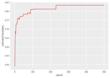
Figure 1: Estimated purified region on Lost.

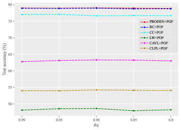
Figure 2: Hyper-parameter sensitivity on CIFAR-10.

4.4 Further Analysis

In addition, to analysis the purified region in Theorem 3.2, we employ the confidence predictions of $f(\bm{x},\tilde{\bm{\theta}})$ (the network in Section 4.1) as the posterior and plot the curve of the estimated purified region in every epoch on Lost in Figure 1. We can see that although the estimated purified region would be not accurate enough, the curve could show that the trend of continuous increase for the purified region.

As the framework of Pop is flexible for the loss function, we integrate the proposed method with the previous methods for instance-independent PLL including Proden, RC, CC, Lw, Cavl and Clpl. In this subsection, we empirically prove that the previous methods for instance-independent PLL could be promoted to achieve better performance after integrating with Pop.

Table 3 and Table 4 report the classification accuracy of each method for instance-independent PLL and its variant integrated with Pop on benchmark datasets corrupted by the ID generating procedure and the real-world datasets, respectively. We didn’t use any data augmentation on benchmark datasets in this part of experiments. As shown in Table 3 and Table 4, the approaches integrated with Pop including Proden+Pop, RC+Pop, CC+Pop , Lw+Pop, Cavl+Pop and Clpl+Pop achieve superior performance against original method, which clearly validates the usefulness of Pop framework for improving performance for ID PLL.

Figure 2 illustrates the variant integrated with Pop performs under different hyper-parameter configurations on CIFAR-10 while similar observations are also made on other data sets. The hyper-parameter sensitivity on other datasets could be founded in Appendix A.4. As shown in Figure 2, it is obvious that the performance of the variant integrated with Pop is relatively stable across a broad range of each hyper-parameter. This property is quite desirable as Pop framework could achieve robust classification performance.

The ablation studies on the warm-up round are shown in Table 5. These results show that the performance of our method does not rely on the warm-up strategy.

5 Conclusion

In this paper, the problem of partial label learning is studied where a novel approach Pop is proposed. we consider ID partial label learning and propose a theoretically-guaranteed approach, which could train the classifier with progressive purification of the candidate labels and is theoretically guaranteed to eventually approximates the Bayes optimal classifier for ID PLL. Experiments on benchmark and real-world datasets validate the effectiveness of the proposed method. If PLL methods become very effective, the need for exactly annotated data would be significantly reduced.

6 Acknowledgments

This research was supported by the National Key Research & Development Plan of China (No. 2021ZD0114202), the National Science Foundation of China (62206050, 62125602, and 62076063), China Postdoctoral Science Foundation (2021M700023), Jiangsu Province Science Foundation for Youths (BK20210220), Young Elite Scientists Sponsorship Program of Jiangsu Association for Science and Technology (TJ-2022-078), and the Big Data Computing Center of Southeast University.

Appendix A Appendix

A.1 Proofs of Theorem 1

Assume that there exists a set $L(e)$ for all $\bm{x}\in L(e)$ which satisfies $y^{\bm{x}}=\arg\max_{j}f_{j}(\bm{x})$ and $p(y^{\bm{x}}|\bm{x})-p(o|\bm{x})\geq e$, we have

$$\mathbb{E}_{(\bm{z},S)\sim\tilde{p}(\bm{z},S_{\text{new}})}\left[\mathbf{1}_{\{{j\neq h^{\star}(\bm{z})}\}}\Big{|}p(y^{\bm{z}}|\bm{z})-p(o|\bm{z})\geq p(y^{\bm{x}}|\bm{x})-p(o|\bm{x}){,~{}j\in S_{\bm{z}}}\right]=0$$ (9)

Let $e_{\text{new}}$ be the new boundary and $\frac{\epsilon}{6l\alpha}(p(y^{\bm{x}}|\bm{x})-e)\leq e-e_{\text{new}}\leq\frac{\epsilon}{3l\alpha}(p(y^{\bm{x}}|\bm{x})-e)$. As the probability density function $d(u)$ of the margin $u(\bm{x})=p(y^{\bm{x}}|\bm{x})-p(o|\bm{x})$ is bounded by $c_{\star}<d(u)<c^{\star}$, we have the following result for $\bm{x}$ that satisfies $p(y^{\bm{x}}|\bm{x})-p(o|\bm{x})\geq e_{\text{new}}$

$$\mathbb{E}_{(\bm{z},S)\sim\tilde{p}(\bm{z},S_{\text{new}})}\left[\mathbf{1}_{\{j\neq h^{\star}(\bm{z})\}}\Big{|}{j\in S_{\bm{z}},}p(y^{\bm{z}}|\bm{z})-p(o|\bm{z})\geq p(y^{\bm{x}}|\bm{x})-p(o|\bm{x})\right]$$ (10)

$$\leq \mathbb{E}_{(\bm{z},S)\sim\tilde{p}(\bm{z},S_{\text{new}})}\left[\mathbf{1}_{\{j\neq h^{\star}(\bm{z})\}}\Big{|}p(y^{\bm{z}}|\bm{z})-p(o|\bm{z})\geq p(y^{\bm{x}}|\bm{x})-p(o|\bm{x})\right]$$

$$= \mathbb{P}_{\bm{z}}\left[j\neq h^{\star}(\bm{z})\Big{|}p(y^{\bm{z}}|\bm{z})-p(o|\bm{z})\geq p(y^{\bm{x}}|\bm{x})-p(o|\bm{x})\right]$$

$$= \frac{\mathbb{P}_{\bm{z}}\left[j\neq h^{\star}(\bm{z}),p(y^{\bm{z}}|\bm{z})-p(o|\bm{z})\geq p(y^{\bm{x}}|\bm{x})-p(o|\bm{x})\right]}{\mathbb{P}_{\bm{z}}\left[p(y^{\bm{z}}|\bm{z})-p(o|\bm{z})\geq p(y^{\bm{x}}|\bm{x})-p(o|\bm{x})\right]}$$

$$\leq \frac{\mathbb{P}_{\bm{z}}\left[j\neq h^{\star}(\bm{z}),p(y^{\bm{z}}|\bm{z})-p(o|\bm{z})\geq e\right]}{\mathbb{P}_{\bm{z}}\left[p(y^{\bm{z}}|\bm{z})-p(o|\bm{z})\geq p(y^{\bm{x}}|\bm{x})-p(o|\bm{x})\right]}+\frac{\mathbb{P}_{\bm{z}}\left[j\neq h^{\star}(\bm{z}),e_{\text{new}}\leq p(y^{\bm{z}}|\bm{z})-p(o|\bm{z})<e\right]}{\mathbb{P}_{\bm{z}}\left[p(y^{\bm{z}}|\bm{z})-p(o|\bm{z})\geq p(y^{\bm{x}}|\bm{x})-p(o|\bm{x})\right]}$$

$$= \frac{\mathbb{P}_{\bm{z}}\left[j\neq h^{\star}(\bm{z}),p(y^{\bm{z}}|\bm{z})-p(o|\bm{z})\geq e\right]}{\mathbb{P}_{\bm{z}}\left[p(y^{\bm{z}}|\bm{z})-p(o|\bm{z})\geq e\right]}\frac{\mathbb{P}_{\bm{z}}\left[p(y^{\bm{z}}|\bm{z})-p(o|\bm{z})\geq e\right]}{\mathbb{P}_{\bm{z}}\left[p(y^{\bm{z}}|\bm{z})-p(o|\bm{z})\geq p(y^{\bm{x}}|\bm{x})-p(o|\bm{x})\right]}$$

$$+\frac{\mathbb{P}_{\bm{z}}\left[j\neq h^{\star}(\bm{z}),e_{\text{new}}\leq p(y^{\bm{z}}|\bm{z})-p(o|\bm{z})<e\right]}{\mathbb{P}_{\bm{z}}\left[p(y^{\bm{z}}|\bm{z})-p(o|\bm{z})\geq p(y^{\bm{x}}|\bm{x})-p(o|\bm{x})\right]}$$

$$= \underbrace{\mathbb{E}_{(\bm{z},S)\sim\tilde{p}(\bm{z},S)}\left[\mathbf{1}_{\{h(\bm{z})\neq y^{\bm{z}}\}}\Big{|}p(y^{\bm{z}}|\bm{z})-p(o|\bm{z})\geq e\right]}_{=0\text{(According to Eq. (\ref{1}))}}\frac{\mathbb{P}_{\bm{z}}\left[p(y^{\bm{z}}|\bm{z})-p(o|\bm{z})\geq e\right]}{\mathbb{P}_{\bm{z}}\left[p(y^{\bm{z}}|\bm{z})-p(o|\bm{z})\geq p(y^{\bm{x}}|\bm{x})-p(o|\bm{x})\right]}$$

$$+\frac{\mathbb{P}_{\bm{z}}\left[j\neq y^{\bm{z}},e_{\text{new}}\leq p(y^{\bm{z}}|\bm{z})-p(o|\bm{z})<e\right]}{\mathbb{P}_{\bm{z}}\left[p(y^{\bm{z}}|\bm{z})-p(o|\bm{z})\geq p(y^{\bm{x}}|\bm{x})-p(o|\bm{x})\right]}$$

$$= \frac{\mathbb{P}_{\bm{z}}\left[e_{\text{new}}\leq p(y^{\bm{z}}|\bm{z})-p(o|\bm{z})<e\right]}{\mathbb{P}_{\bm{z}}\left[p(y^{\bm{z}}|\bm{z})-p(o|\bm{z})\geq p(y^{\bm{x}}|\bm{x})-p(o|\bm{x})\right]}$$

$$\leq \frac{c^{\star}(e-e_{\text{new}})}{c_{\star}\left(p(y^{\bm{x}}|\bm{x})-e\right)}.$$

Due to that $\frac{\epsilon}{6l\alpha}(p(y^{\bm{x}}|\bm{x})-e)\leq e-e_{\text{new}}\leq\frac{\epsilon}{3l\alpha}(p(y^{\bm{x}}|\bm{x})-e)$ holds, we can further relax Eq. (10) as follows:

$$\mathbb{E}_{(\bm{z},S)\sim\tilde{p}(\bm{z},S_{\text{new}})}\left[\mathbf{1}_{\{j\neq h^{\star}(\bm{z})\}}\Big{|}j\in S_{\bm{z}},p(y^{\bm{z}}|\bm{z})-p(o|\bm{z})\geq p(y^{\bm{x}}|\bm{x})-p(o|\bm{x})\right]$$ (11)

$$\leq\frac{c^{*}(e-e_{\text{new}})}{c_{*}\left(p(y^{\bm{x}}|\bm{x})-e\right)}$$

$$\leq\frac{c^{*}}{c_{*}\left(p(y^{\bm{x}}|\bm{x})-e\right)}\frac{\epsilon}{3l\alpha}(p(y^{\bm{x}}|\bm{x})-e)$$

$$=\frac{\epsilon}{3\alpha}.$$

Then, we can find that the assumption that the gap between $f_{j}(\bm{x})$ and $f^{\star}_{j}(\bm{x})$ should be controlled by the risk at point $\bm{z}$ implies:

$$\left|f_{j}(\bm{x})-f^{\star}_{j}(\bm{z})\right|$$ (12)

$$\leq \,\alpha\mathbb{E}_{(\bm{z},S)\sim\tilde{p}(\bm{z},S_{\text{new}})}\left[\mathbbm{1}_{\{h(\bm{z})\neq y^{\bm{z}}\}}\Big{|}p(y^{\bm{z}}|\bm{z})-p(o|\bm{z})\geq p(y^{\bm{x}}|\bm{x})-p(o|\bm{x})\right]+\frac{\epsilon}{6}$$

$$\leq \,\alpha\frac{\epsilon}{3\alpha}+\frac{\epsilon}{6}$$

$$\leq \,\frac{\epsilon}{2}.$$

Hence, for $\bm{x}$ s.t. $p(y^{\bm{x}}|\bm{x})-p(o|\bm{x})\geq e_{\text{new}}$, according to Eq. (12) we have

$$f_{y^{\bm{x}}}(\bm{x})-f_{j\neq y^{\bm{x}}}(\bm{x}) \geq(p(y=y^{\bm{x}}|\bm{x})-\frac{\epsilon}{2})-(p(y=j|\bm{x})+\frac{\epsilon}{2})$$ (13)

$$=p(y=y^{\bm{x}}|\bm{x})-p(y=j|\bm{x})-\epsilon$$

$$\geq p(y=y^{\bm{x}}|\bm{x})-p(o|\bm{x})-\epsilon$$

$$\geq e_{\text{new}}-\epsilon$$

$$\geq 0,$$

which means that ${}_{j}(\bm{x})$ will be the same label as $h^{\star}$ and thus the level set $L(e_{\text{new}})$ is pure for $f$. Meanwhile, the choice of $e_{\text{new}}$ ensures that

$$p(y^{\bm{x}}|\bm{x})-e_{\text{new}} \geq p(y^{\bm{x}}|\bm{x})-(e-\frac{\epsilon}{6l\alpha}(p(y^{\bm{x}}|\bm{x})-e))$$ (14)

$$=p(y^{\bm{x}}|\bm{x})-e+\frac{\epsilon}{6l\alpha}(p(y^{\bm{x}}|\bm{x})-e)$$

$$=(1+\frac{\epsilon}{6l\alpha})(p(y^{\bm{x}}|\bm{x})-e).$$

Here, the proof of Theorem 1 has been completed.

A.2 Details of Eq. (5)

If $f_{m}(\bm{x})-f_{j\neq m}\geq e+\epsilon$, according to Eq. (12) we have:

$$p(y^{\bm{x}}|\bm{x}) \geq p(y=m|\bm{x})$$ (15)

$$=p(y=j|\bm{x})+p(y=m|\bm{x})-p(y=j|\bm{x})$$

$$\geq p(y=j|\bm{x})+p(y=m|\bm{x})-p(y=j|\bm{x})$$

$$\geq p(y=j|\bm{x})+(f_{m}(\bm{x})-\frac{\epsilon}{2})-(f_{j}(\bm{x})+\frac{\epsilon}{2})$$

$$=p(y=j|\bm{x})+(f_{m}(\bm{x})-f_{j}(\bm{x}))-\epsilon$$

$$\geq p(y=j|\bm{x})+(e+\epsilon)-\epsilon$$

$$=p(y=j|\bm{x})+e.$$

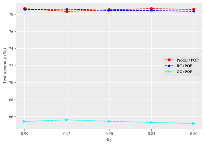
Figure 3: Hyper-parameter sensitivity on Lost.

A.3 Proofs of Theorem 2

To begin with, we prove that there exists at least a level set $L(e_{0})$ pure to $f_{0}$. Considering $\bm{x}$ satisfies $p(y^{\bm{x}}|\bm{x})-p(o|\bm{x})\geq e_{0}$, we have $\mathbb{P}_{\bm{z}}\left[j\neq h^{\star}(\bm{z})\Big{|}j\in S_{\bm{z}},p(y^{\bm{z}}|\bm{z})-p(o|\bm{z})\geq e_{0}\right]\leq p(y^{\bm{z}}|\bm{z})-e_{0}+\xi^{j}(\bm{z})$. Due to the assumption $|f_{j}(\bm{x})-f^{\star}_{j}(\bm{x})|\leq\alpha\mathbb{E}_{(\bm{z},S)\sim\tilde{p}(\bm{z},S)}\left[\mathbf{1}_{\{j\neq h^{\star}(\bm{z})\}}\Big{|}j\in S_{\bm{z}},p(y^{\bm{z}}|\bm{z})-p(o|\bm{z})\geq p(y^{\bm{x}}|\bm{x})-p(o|\bm{x})\right]+\frac{\epsilon}{6}$, it suffices to satisfy $\alpha(p(y^{\bm{x}}|\bm{x})-e_{0}+\xi)+\frac{\epsilon}{6}\leq e_{0}$ to ensure that $f_{j}(\bm{x})$ has the same prediction with $h^{\star}$ when $p(y^{\bm{x}}|\bm{x})-p(o|\bm{x})\geq e_{0}$. Since we have $\xi^{j}(\bm{x})\leq p(y=j|\bm{x})t\leq p(y^{\bm{x}}|\bm{x})t$, by choosing $e_{0}\geq\frac{(1+t)\alpha+\frac{\epsilon}{6}}{1+\alpha}\geq\frac{(1+t)\alpha p(y^{\bm{x}}|\bm{x})+\frac{\epsilon}{6}}{1+\alpha}$ one can ensure that initial $f_{0}$ has a pure $L(e_{0})$-level set.

Then in the rest of the iterations we ensure the level set $p(y^{\bm{z}}|\bm{z})-p(o|\bm{z})\geq e$ is pure. We decrease $e$ by a reasonable factor to avoid incurring too many corrupted labels while ensuring enough progress in label purification, i.e. $\frac{\epsilon}{6l\alpha}(p(y^{\bm{x}}|\bm{x})-e)\leq e-e_{\text{new}}\leq\frac{\epsilon}{3l\alpha}(p(y^{\bm{x}}|\bm{x})-e)$, such that in the level set $p(y^{\bm{x}}|\bm{x})-p(o|\bm{x})\geq e_{\text{new}}$ we have $|f_{j}(\bm{x})-f^{\star}_{j}(\bm{x})|\leq\frac{\epsilon}{2}$. This condition ensures the correctness of flipping when $e\geq\epsilon$. The the purified region cannot be improved once $e<\epsilon$ since there is no guarantee that $f_{j}(\bm{x})$ has consistent label with $h^{\star}$ when $p(y^{\bm{x}}|\bm{x})-p(o|\bm{x})<\epsilon$ and $|f_{j}(\bm{x})-f^{\star}_{j}(\bm{x})|\leq\frac{\epsilon}{2}$. To get the largest purified region, we can set $e_{\text{end}}=\epsilon$. Since the probability density function $d(u)$ of the margin $u(\bm{x})=p(y^{\bm{x}}|\bm{x})-p(o|\bm{x})$ is bounded by $c_{\star}\leq d(u)\leq c^{\star}$, we have:

$$\mathbb{P}_{\bm{x}\sim D}[y_{f_{final}(\bm{x})}\neq h^{\star}] \leq\mathbb{P}[p(y^{\bm{x}}|\bm{x})-p(o|\bm{x})<e_{\text{end}}]$$ (16)

$$=\mathbb{P}_{\bm{x}\sim D}[p(y^{\bm{x}}|\bm{x})-p(o|\bm{x})<\epsilon]$$

$$\leq c^{\star}\epsilon.$$

Then $\mathbb{P}_{\bm{x}\sim D}[y_{f_{final}(\bm{x})}=h^{\star}]=1-\mathbb{P}_{\bm{x}\sim D}[y_{f_{final}(\bm{x})}\neq h^{\star}]\geq 1-c^{\star}\epsilon$.

The rest of the proof is the total round $R\geq\frac{6\alpha l}{\epsilon}\log(\frac{1-\epsilon}{\frac{1}{c}-e_{0}})$, which follows from the fact that each round of label flipping improves the the purified region by a factor of $(1+\frac{\epsilon}{6l\alpha})$:

$$\left(1+\frac{\epsilon}{6l\alpha}\right)^{R}\left(p(y^{\bm{x}}|\bm{x})-e_{0}\right)\geq p(y^{\bm{x}}|\bm{x})-\epsilon$$ (17)

$$\Rightarrow\left(1+\frac{\epsilon}{6l\alpha}\right)^{R}\geq\frac{p(y^{\bm{x}}|\bm{x})-\epsilon}{p(y^{\bm{x}}|\bm{x})-e_{0}}$$

$$\Rightarrow R\log\left(1+\frac{\epsilon}{6l\alpha}\right)\geq\log\left(\frac{p(y^{\bm{x}}|\bm{x})-\epsilon}{p(y^{\bm{x}}|\bm{x})-e_{0}}\right)$$

$$\Rightarrow R\frac{\epsilon}{6l\alpha}\geq R\log\left(1+\frac{\epsilon}{6l\alpha}\right)\geq\log\left(\frac{p(y^{\bm{x}}|\bm{x})-\epsilon}{p(y^{\bm{x}}|\bm{x})-e_{0}}\right)$$

$$\Rightarrow R\geq\frac{6l\alpha}{\epsilon}\log\left(\frac{p(y^{\bm{x}}|\bm{x})-\epsilon}{p(y^{\bm{x}}|\bm{x})-e_{0}}\right)\geq\frac{6l\alpha}{\epsilon}\log(\frac{1-\epsilon}{\frac{1}{c}-e_{0}}).$$

Table 6: Characteristic of the benchmark datasets corrupted by the ID generation process.

Dataset	#Train	#Test	#Features	#Class Labels	avg. #CLs
MNIST	60000	10000	784	10	8.71
Fashion-MNIST	60,000	10,000	784	10	3.46
Kuzushiji-MNIST	60,000	10,000	784	10	3.87
CIFAR-10	50,000	10,000	3,072	10	3.68
CIFAR-100	50,000	10,000	3,072	100	4.64

Table 7: Characteristic of the real-world PLL datasets.

Dataset	#Train	#Test	#Features	#Class Labels	avg. #CLs	Task Domain
Lost	898	224	108	16	2.23	automatic face naming (Cour et al., 2011)
MSRCv2	1,406	352	48	23	3.16	object classification (Liu & Dietterich, 2012)
Mirflickr	2224	556	1536	14	2.76	web image classification (Huiskes & Lew, 2008)
BirdSong	3,998	1,000	38	13	2.18	bird song classification (Briggs et al., 2012)
Malagasy	4243	1069	384	44	8.35	POS Tagging (Garrette & Baldridge, 2013)
Soccer Player	13,978	3,494	279	171	2.09	automatic face naming (Zeng et al., 2013)
Yahoo! News	18,393	4,598	163	219	1.91	automatic face naming (Guillaumin et al., 2010)

A.4 Details of Experiments

We collect five widely used benchmark datasets including MNIST (LeCun et al., 1998), Kuzushiji-MNIST (Clanuwat et al., 2018), Fashion-MNIST (Xiao et al., 2017), CIFAR-10 (Krizhevsky & Hinton, 2009), CIFAR-100 (Krizhevsky & Hinton, 2009). In addition, seven real-world PLL datasets which are collected from different application domains are used, including Lost (Cour et al., 2011), Soccer Player (Zeng et al., 2013), Yahoo!News (Guillaumin et al., 2010) from automatic face naming,, MSRCv2 (Liu & Dietterich, 2012) from object classification, Malagasy (Garrette & Baldridge, 2013) from POS tagging, Mirflickr (Huiskes & Lew, 2008) from web image classification, and BirdSong (Briggs et al., 2012) from bird song classification. Figure 3 illustrates the variant integrated with Pop performs under different hyper-parameter configurations on Lost.

The average number of candidate labels (avg. #CLs) for each benchmark dataset corrupted by the ID generation process is recorded in Table-6 and the average number of candidate labels (avg. #CLs) for each real-world PLL dataset is recorded in Table-7.

References

- Bartlett et al. (2006) Bartlett, P. L., Jordan, M. I., and McAuliffe, J. D. Convexity, classification, and risk bounds. Journal of the American Statistical Association, 101(473):138?156, 2006.
- Blei et al. (2017) Blei, D. M., Kucukelbir, A., and McAuliffe, J. D. Variational inference: A review for statisticians. Journal of the American Statistical Association, 112(518):859–877, 2017.
- Briggs et al. (2012) Briggs, F., Fern, X. Z., and Raich, R. Rank-loss support instance machines for miml instance annotation. In Proceedings of 18th ACM SIGKDD International Conference on Knowledge Discovery and Data Mining (KDD’12), pp. 534–542, 2012.
- Chen et al. (2014) Chen, Y., Patel, V. M., Pillai, J. K., Chellappa, R., and Phillips, P. J. Ambiguously labeled learning using dictionaries. IEEE Transactions on Information Forensics and Security, 9(12):2076–2088, 2014.
- Clanuwat et al. (2018) Clanuwat, T., Bober-Irizar, M., Kitamoto, A., Lamb, A., Yamamoto, K., and Ha, D. Deep learning for classical japanese literature. arXiv preprint arXiv:1812.01718, 2018.
- Cour et al. (2011) Cour, T., Sapp, B., and Taskar, B. Learning from partial labels. Journal of Machine Learning Research, 12(5):1501–1536, 2011.
- Feng & An (2019) Feng, L. and An, B. Partial label learning with self-guided retraining. In Proceedings of 33rd AAAI Conference on Artificial Intelligence (AAAI’19), pp. 3542–3549, 2019.
- Feng et al. (2020a) Feng, L., Kaneko, T., Han, B., Niu, G., An, B., and Sugiyama, M. Learning with multiple complementary labels. In Proceedings of 37th International Conference on Machine Learning (ICML’20), pp. 3072–3081, 2020a.
- Feng et al. (2020b) Feng, L., Lv, J., Han, B., Xu, M., Niu, G., Geng, X., An, B., and Sugiyama, M. Provably consistent partial-label learning. In Advances in Neural Information Processing Systems 33 (NeurIPS’20), pp. 10948–10960, 2020b.
- Garrette & Baldridge (2013) Garrette, D. and Baldridge, J. Learning a part-of-speech tagger from two hours of annotation. In Proceedings of the 2013 Conference of the North American Chapter of the Association for Computational Linguistics: Human Language Technologies, pp. 138–147, 2013.
- Gneiting & Raftery (2007) Gneiting, T. and Raftery, A. E. Strictly proper scoring rules, prediction, and estimation. Journal of the American statistical Association, 102(477):359–378, 2007.
- Guillaumin et al. (2010) Guillaumin, M., Verbeek, J., and Schmid, C. Multiple instance metric learning from automatically labeled bags of faces. In Proceedings of 11th European Conference on Computer Vision (ECCV’10), volume 6311, pp. 634–647, 2010.
- Huiskes & Lew (2008) Huiskes, M. J. and Lew, M. S. The mir flickr retrieval evaluation. In Proceedings of the 1st ACM international conference on Multimedia information retrieval, pp. 39–43, 2008.
- Hüllermeier & Beringer (2006) Hüllermeier, E. and Beringer, J. Learning from ambiguously labeled examples. Intelligent Data Analysis, 10(5):419–439, 2006.
- Ishida et al. (2017) Ishida, T., Niu, G., Hu, W., and Sugiyama, M. Learning from complementary labels. In Advances in Neural Information Processing Systems 30 (NeurIPS’17), pp. 5639–5649, 2017.
- Ishida et al. (2019) Ishida, T., Niu, G., Menon, A. K., and Sugiyama, M. Complementary-label learning for arbitrary losses and models. In Proceedings of 36th International Conference on Machine Learning (ICML’19), pp. 2971–2980, 2019.
- Jin & Ghahramani (2003) Jin, R. and Ghahramani, Z. Learning with multiple labels. In Advances in Neural Information Processing Systems 16 (NeurIPS’03), pp. 921–928, 2003.
- Krizhevsky & Hinton (2009) Krizhevsky, A. and Hinton, G. Learning multiple layers of features from tiny images. 2009.
- LeCun et al. (1998) LeCun, Y., Bottou, L., Bengio, Y., and Haffner, P. Gradient-based learning applied to document recognition. Proceedings of the IEEE, 86(11):2278–2324, 1998.
- Liu & Dietterich (2012) Liu, L. and Dietterich, T. G. A conditional multinomial mixture model for superset label learning. In Advances in Neural Information Processing Systems 25 (NIPS’12), pp. 548–556, 2012.
- Luo & Orabona (2010) Luo, J. and Orabona, F. Learning from candidate labeling sets. In Advances in Neural Information Processing Systems 23 (NeurIPS’10), pp. 1504–1512, 2010.
- Lv et al. (2020) Lv, J., Xu, M., Feng, L., Niu, G., Geng, X., and Sugiyama, M. Progressive identification of true labels for partial-label learning. In Proceedings of 37th International Conference on Machine Learning (ICML’20), pp. 6500–6510, 2020.
- Lyu et al. (2022) Lyu, G., Wu, Y., and Feng, S. Partial label learning by semantic difference maximization. In Proceedings of 31st International Joint Conference on Artificial Intelligence, 2022.
- Mohri et al. (2018) Mohri, M., Rostamizadeh, A., and Talwalkar, A. Foundations of machine learning. MIT press, 2018.
- Nguyen & Caruana (2008) Nguyen, N. and Caruana, R. Classification with partial labels. In Proceedings of 14th ACM SIGKDD Conference on Knowledge Discovery and Data Mining (KDD’08), pp. 551–559, 2008.
- Patrini et al. (2017) Patrini, G., Rozza, A., Menon, A. K., Nock, R., and Qu, L. Making deep neural networks robust to label noise: A loss correction approach. In Proceedings of 30th IEEE Conference on Computer Vision and Pattern Recognition (CVPR’17), pp. 1944–1952, 2017.
- Reidand & Williamson (2010) Reidand, M. D. and Williamson, R. C. Composite binary losses. The Journal of Machine Learning Research, 11:2387–2422, 2010.
- Tang & Zhang (2017) Tang, C. and Zhang, M. Confidence-rated discriminative partial label learning. In Proceedings of 31st AAAI Conference on Artificial Intelligence (AAAI’17), pp. 2611–2617, 2017.
- Wang et al. (2022) Wang, H., Xiao, R., Li, Y., Feng, L., Niu, G., Chen, G., and Zhao, J. Pico: Contrastive label disambiguation for partial label learning. In Proceedings of the 10th International Conference on Learning Representations, 2022.
- Wen et al. (2021) Wen, H., Cui, J., Hang, H., Liu, J., Wang, Y., and Lin, Z. Leveraged weighted loss for partial label learning. In Proceedings of 36th International Conference on Machine Learning (ICML’21), pp. 11091–11100, 2021.
- Wu et al. (2022) Wu, D.-D., Wang, D.-B., and Zhang, M.-L. Revisiting consistency regularization for deep partial label learning. In International Conference on Machine Learning, pp. 24212–24225. PMLR, 2022.
- Wu & Sugiyama (2021) Wu, Z. and Sugiyama, M. Learning with proper partial labels. arXiv preprint arXiv:2112.12303, 2021.
- Xia et al. (2020) Xia, X., Liu, T., Han, B., Wang, N., Gong, M., Liu, H., Niu, G., Tao, D., and Sugiyama, M. Part-dependent label noise: Towards instance-dependent label noise. In Advances in Neural Information Processing Systems 33 (NeurIPS’20), pp. 7597–7610, 2020.
- Xiao et al. (2017) Xiao, H., Rasul, K., and Vollgraf, R. Fashion-mnist: a novel image dataset for benchmarking machine learning algorithms. arXiv preprint arXiv:1708.07747, 2017.
- Xu et al. (2019) Xu, N., Lv, J., and Geng, X. Partial label learning via label enhancement. In Proceedings of 33rd AAAI Conference on Artificial Intelligence (AAAI’19), pp. 5557–5564, 2019.
- Xu et al. (2021a) Xu, N., Liu, Y.-P., and Geng, X. Label enhancement for label distribution learning. IEEE Transactions on Knowledge and Data Engineering, 33(4):1632 – 1643, 2021a.
- Xu et al. (2021b) Xu, N., Qiao, C., Geng, X., and Zhang, M. Instance-dependent partial label learning. In Advances in Neural Information Processing Systems 34 (NeurIPS’21), 2021b.
- Xu et al. (2022) Xu, N., Qiao, C., Lv, J., Geng, X., and Zhang, M.-L. One positive label is sufficient: Single-positive multi-label learning with label enhancement. In Advances in Neural Information Processing Systems, pp. 21765–21776, New Orleans, LA, 2022.
- Xu et al. (2023) Xu, N., Shu, J., Zheng, R., Geng, X., Meng, D., and Zhang, M. Variational label enhancement. IEEE Trans. Pattern Anal. Mach. Intell., 45(5):6537–6551, 2023.
- Yang et al. (2017) Yang, Y., Zhan, D., Fan, Y., Jiang, Y., and Zhou, Z. Deep learning for fixed model reuse. In Proceedings of the Thirty-First AAAI Conference on Artificial Intelligence, pp. 2831–2837, San Francisco, CA, 2017.
- Yao et al. (2020a) Yao, Y., Gong, C., Deng, J., Chen, X., Wu, J., and Yang, J. Deep discriminative cnn with temporal ensembling for ambiguously-labeled image classification. In Proceedings of 34th AAAI Conference on Artificial Intelligence (AAAI’20), pp. 12669–12676, 2020a.
- Yao et al. (2020b) Yao, Y., Gong, C., Deng, J., and Yang, J. Network cooperation with progressive disambiguation for partial label learning. In The European Conference on Machine Learning and Principles and Practice of Knowledge Discovery in Databases (ECML-PKDD), pp. 471–488, 2020b.
- Yu et al. (2018) Yu, X., Liu, T., Gong, M., and Tao, D. Learning with biased complementary labels. In Proceedings of 15th European Conference on Computer Vision (ECCV’18), pp. 68–83, 2018.
- Zagoruyko & Komodakis (2016) Zagoruyko, S. and Komodakis, N. Wide residual networks. arXiv preprint arXiv:1605.07146, 2016.
- Zeng et al. (2013) Zeng, Z., Xiao, S., Jia, K., Chan, T., Gao, S., Xu, D., and Ma, Y. Learning by associating ambiguously labeled images. In Proceedings of 26th IEEE Conference on Computer Vision and Pattern Recognition (CVPR’13), pp. 708–715, 2013.
- Zhang et al. (2017a) Zhang, C., Bengio, S., Hardt, M., Recht, B., and Vinyals, O. Understanding deep learning requires rethinking generalization. In International Conference on Learning Representations, 2017a.
- Zhang et al. (2021a) Zhang, F., Feng, L., Han, B., Liu, T., Niu, G., Qin, T., and Sugiyama, M. Exploiting class activation value for partial-label learning. In International Conference on Learning Representations, 2021a.
- Zhang & Yu (2015) Zhang, M. and Yu, F. Solving the partial label learning problem: An instance-based approach. In Proceedings of 24th International Joint Conference on Artificial Intelligence (IJCAI’15), pp. 4048–4054, 2015.
- Zhang et al. (2016) Zhang, M., Zhou, B., and Liu, X. Partial label learning via feature-aware disambiguation. In Proceedings of 22nd ACM SIGKDD International Conference on Knowledge Discovery and Data Mining (KDD’16), pp. 1335–1344, 2016.
- Zhang et al. (2017b) Zhang, M., Yu, F., and Tang, C. Disambiguation-free partial label learning. IEEE Transactions on Knowledge and Data Engineering, 29(10):2155–2167, 2017b.
- Zhang et al. (2021b) Zhang, Y., Zheng, S., Wu, P., Goswami, M., and Chen, C. Learning with feature-dependent label noise: A progressive approach. In Proceedings of 9th International Conference on Learning Representations (ICLR’21), 2021b.