Decentralized temperature and storage volume control in multi-producer district heating*

Abstract

Modern district heating technologies have a great potential to make the energy sector more flexible and sustainable due to their capabilities to use energy sources of varied nature and to efficiently store energy for subsequent use. Central control tasks within these systems for the efficient and safe distribution of heat refer to the stabilization of overall system temperatures and the regulation of storage units state of charge. These are challenging goals when the networked and nonlinear nature of district heating system models is taken into consideration. In this letter, for district heating systems with multiple, distributed heat producers, we propose a decentralized control scheme to provably meet said tasks stably.

Index terms: Stability of nonlinear systems; Lyapunov methods; Energy systems.

I Introduction

District heating systems (DHSs) distribute heat from heating stations, conventionally a single combined heat and power plant, towards clusters of consumers within a neighborhood or a small city using a network of underground insulated pipelines [1]. The newest generation DHSs have the potential to improve the sustainability of a fossil fuel-dependent heating sector by increasing the share of distributed generations units based on renewables (e.g., geothermal or solar thermal) as well as units based on residual heat from some industrial processes. Such units can be flexibly incorporated with the support of heat storage devices (typically water tanks) [1] (see also [2, 3]).

Heat distribution in DHSs, in the face of varying weather conditions and heat demand profiles, is supported by a control system in charge of regulating the supply (return) temperature of heat producers (consumers) and the state of charge of storage units [4, 5]. This is done by adjusting producers’ power injections and the overall system’s flow rates so that the heat supply matches the demand and the system temperatures stay within prescribed domains. Optimal, predictive (and centralized) control of DHSs has been addressed for systems without ([6, 7]) and with ([8]) heat storage units. Supply temperature control and storage volume regulation is performed in [9] on a dynamic, nonlinear system model of a DH system comprising a single heating station with an adjacent storage tank. The control design is based on the internal model principle and offers closed-loop stability guarantees and robustness against uncertainty of some parameters. For a similar system model, which does not consider storage units, but does consider transport dynamics of the distribution network (codified as a delay), a control design based on Lyapunov-Krasovksii theory to achieve (supply and return) temperature regulation is reported in [10]. Recently, the control of supply temperatures of heating stations was investigated in [11] using passivity-based design within the context of electro-thermal microgrids consisting of distributed generation units. Optimal, open-loop end-user temperature control is investigated in [12] via numerical simulations of a DH system with multiple prosumers. Focused on the hydraulic dynamics, i.e., neglecting the thermal behavior, the works [13, 14, 15] address pressure regulation on single producer DH systems and [16, 17] consider flow and volume control in the multi-producer setting.

I-A Contributions

In Section II, we describe the setup of the considered DH system, which features multiple, distributed producers with heat storage capabilities. We then develop a (modular) dynamic model that describes the behavior of the overall system temperatures, including heat exchangers and storage tanks, and the supply and return layers of the distribution network. Our main contribution is in Section III, where we design novel decentralized controllers to regulate supply temperature of heat producers, the temperature and volume of the storage tanks and the return temperature of heat consumers. Stability analysis of the overall closed-loop system concludes the section. Note that the simultaneous treatment of the mentioned tasks, using decentralized controllers and with the considered system setup is not addressed in the above cited works.

I-B Notation (including table of variables)

The symbol $\mathbb{R}$ denotes the set of real numbers. For a vector $x\in\mathbb{R}^{n}$, $x_{i}$ denotes its $i$th component, i.e., $x=[x_{1},\dots,x_{n}]^{\top}$; moreover, $\mathbf{sign}(x)=[\text{sign}(x_{1}),\dots,\text{sign}(x_{n})]^{\top}$, with $\text{sign}(0)=0$, and $|x|=[|x_{1}|,\dots,|x_{n}|]^{\top}$. An $m\times n$ matrix with all-zero entries is written as $\boldsymbol{0}_{m\times n}$. An $n$-vector of ones is written as $\boldsymbol{1}_{n}$, whereas the identity matrix of size $n$ is represented by $I_{n}$. For any vector $x\in\mathbb{R}^{n}$, we denote by $\mathrm{diag}(x)$ a diagonal matrix with elements $x_{i}$ in its main diagonal. For any time-varying signal $w$, we represent by $\bar{w}$ its steady-state value, if exists. Also, we write time derivatives as $\dot{x}(t)$, and omit the argument $t$ whenever is clear from the context. For conveience, we provide summarize lists of relevant abbreviations and symbols in Tables I and II, respectively.

TABLE I: List of Abbreviations

DHS	district heating system
DN	distribution network
ST	storage tank
HX	heat exchanger
p	identifier for producers
c	identifier for consumers
st	identifier for storage tanks
sh	identifier for hot layer of storage tanks
sc	identifier for cold layer of storage tanks
s	identifier for elements associated to the DN’s supply layer
r	identifier for elements associated to the DN’s return layer

TABLE II: Network Parameters

$\mathcal{G}_{\mathrm{s}}$, $\mathcal{N}_{\mathrm{s}}$, $\mathcal{E}_{\mathrm{s}}$	DH system’s graph, nodes (junctions) and edges (pipes)
	associated to the supply layer
$\mathcal{G}_{\mathrm{r}}$, $\mathcal{N}_{\mathrm{r}}$, $\mathcal{E}_{\mathrm{r}}$	DH system’s graph, nodes (junctions) and edges (pipes)
	associated to the return layer
$P_{\mathrm{p},i}$	power injection by $i$th producer, W
$P_{\mathrm{c},i}$	power extraction by $i$th consumer, W
$q_{\mathrm{p},i}$	flow rate through edge the $i$th producer, $\mathrm{m}^{3}/s$
$q_{\mathrm{st},i}$	flow rate at hot layer outlet (cold layer inlet) of the
	$i$th storage tank, $\mathrm{m}^{3}/s$
$q_{\mathrm{c},i}$	flow rate through edge the $i$th consumer, $\mathrm{m}^{3}/s$
$q_{\mathrm{s},i}$	flow rate through $i\in\mathcal{E}_{\mathrm{s}}$, $\mathrm{m}^{3}/s$
$q_{\mathrm{r},i}$	flow rate through $i\in\mathcal{E}_{\mathrm{r}}$, $\mathrm{m}^{3}/s$
$V_{\mathrm{p},i}$	effective volume of the secondary side of the
	$i$th producer’s HX, $\mathrm{m}^{3}$
$V_{\mathrm{c},i}$	effective volume of the primary side of the
	$i$th consumer’s HX, $\mathrm{m}^{3}$
$V_{\mathrm{sh},i}$	volume of water in the $i$th ST’s hot layer, $\mathrm{m}^{3}$
$V_{\mathrm{c},i}$	volume of water in the $i$th ST’s cold layer, $\mathrm{m}^{3}$
$V_{\mathrm{s},i}$	effective volume of $i\in\mathcal{G}_{\mathrm{s}}$, $\mathrm{m}^{3}$
$V_{\mathrm{r},i}$	effective volume of $i\in\mathcal{G}_{\mathrm{r}}$, $\mathrm{m}^{3}$
$T_{\mathrm{p},i}$	average temperature of the secondary side of the
	$i$th producer’s HX, $~{}^{\circ}\mathrm{C}$
$T_{\mathrm{c},i}$	average temperature of the primary side of the
	$i$th consumer’s HX, $~{}^{\circ}\mathrm{C}$
$T_{\mathrm{sh},i}$	average temperature of the $i$th ST’s hot layer, $~{}^{\circ}\mathrm{C}$
$T_{\mathrm{sc},i}$	average temperature of the $i$th ST’s cold layer, $~{}^{\circ}\mathrm{C}$
$T_{\mathrm{s},i}$	average temperature of the $i\in\mathcal{G}_{\mathrm{s}}$, $~{}^{\circ}\mathrm{C}$
$T_{\mathrm{r},i}$	average temperature of the $i\in\mathcal{G}_{\mathrm{r}}$, $~{}^{\circ}\mathrm{C}$
$\rho$	density of water, $\mathrm{kg}/\mathrm{m}^{3}$
$c_{\mathrm{s.h.}}$	specific heat of water, $\mathrm{J}/\mathrm{kg}~{}^{\circ}\mathrm{C}$
$(\cdot)^{\mathrm{in}}_{i}$	quantity associated to an inlet
$(\cdot)^{\mathrm{out}}_{i}$	quantity associated to an outlet

II System model

II-A Setup and main modeling assumptions

We consider a DH system with multiple, distributed $n_{\mathrm{p}}$ producers and $n_{\mathrm{c}}$ consumers interconnected through a distribution network (DN) that has a supply (hot) layer and return (cold) layer. The specific composition of producers and consumers is shown in Fig. 1. Note that each producer can continuously drain water from the DN’s return layer, heats it through a heat exchanger (HX) and injects the heated stream into the DN’s supply layer. A converse operation follows for consumers.

Following [9], we consider a DH system with stratified storage tanks. Each tank stores a mixture of hot and cold water perfectly separated by a thermocline. The volume of hot water is on top and the cold one at the bottom. It is assumed that there is no heat or mass exchange between the mixtures. Moreover, each storage tank is considered to have two inlet/outlet pairs for hot and cold water, respectively. The topology of storage tanks is shown in Fig. 1. As a simplifying assumption, we consider that each producer is interfaced to the DN via a storage tank. Then, each producer drains water from the cold layer of a storage tank and injects it into the tank’s hot layer. Using the remaining inlet/outlet pair, the tank can fill in its cold layer with water taken from the return layer of the DN. At the same time, the storage tank injects water from its hot layer into the DN’s supply layer. We note that our results can be slightly adjusted to consider producers directly connected to the DN. However, standalone storage tanks, i.e., storage tanks with no immediate access to a heat producer are not considered in this work.

Additional modeling assumptions, some of which are fairly standard in related literature (see, e.g., [9, 10, 12]) are the following (see [18] for more details):

Assumption 1.

(i) the density $\rho>0$ and specific heat $c_{\mathrm{s.h.}}>0$ of water are spatially uniform and constant in time (for ease of notation we take $\rho=c_{\mathrm{s.h.}}=1$); (ii) the flow through any pipe is (spatially) one-dimensional. (iii) each device (pipe, storage tank, junction) is completely filled with water at all times; (iv) the internal energy of any water stream portion depends linearly on its temperature; the overall DH system is leak-free and lossless.

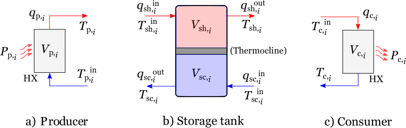
Figure 1: Topologies of producers, consumers and storage tanks [9, 10]: $T_{\chi,i}$, $V_{\chi,i}$, $q_{\chi,i}$ and $P_{\chi,i}$ stand for temperature, volume, flow rate and thermal power associated with the $i$th device $\chi\in\{\mathrm{p},~{}\mathrm{sh},~{}\mathrm{sc},~{}\mathrm{st},~{}\mathrm{c}\}$.

II-B Dynamics of producers and storage tanks

Consider the notation used in Fig. 1. The heat balance at the secondary side of the $i$th producer’s heat exchanger can be written as follows [9], [10]:

$$V_{\mathrm{p},i}\dot{T}_{\mathrm{p},i}=q_{\mathrm{p},i}\left(T_{\mathrm{p},i}^{\mathrm{in}}-T_{\mathrm{p},i}\right)+P_{\mathrm{p},i},$$ (1)

where $q_{\mathrm{p},i}$ and $P_{\mathrm{p},i}$ are considered to be control variables: each $q_{\mathrm{p},i}$ could be controlled in practice independently by a pump in series with the secondary side of the producer’s heat exchanger whereas each $P_{\mathrm{p},i}$ could be controlled independently by adjusting the flow in the primary side (hotter side) of a producer’s heat exchanger (see [9, Appendix A] for additional details).

On the other hand, the heat balance at the hot and cold layer of each storage tank can be written respectively as follows:

$$\frac{\mathrm{d}}{\mathrm{d}t}(V_{\mathrm{sh},i}{T}_{\mathrm{sh},i}) =q_{\mathrm{sh},i}^{\mathrm{in}}T_{\mathrm{sh},i}^{\mathrm{in}}-q_{\mathrm{sh},i}^{\mathrm{out}}T_{\mathrm{sh},i}$$ (2)

$$\frac{\mathrm{d}}{\mathrm{d}t}(V_{\mathrm{sc},i}{T}_{\mathrm{sc},i}) =q_{\mathrm{sc},i}^{\mathrm{in}}T_{\mathrm{sc},i}^{\mathrm{in}}-q_{\mathrm{sc},i}^{\mathrm{out}}T_{\mathrm{sc},i}.$$ (3)

Moreover, the volume dynamics of of the layers of each tank obey the following equations:

$$\dot{V}_{\mathrm{sh},i} =q_{\mathrm{sh},i}^{\mathrm{in}}-q_{\mathrm{sh},i}^{\mathrm{out}}$$ (4)

$$\dot{V}_{\mathrm{sc},i} =q_{\mathrm{sc},i}^{\mathrm{in}}-q_{\mathrm{sc},i}^{\mathrm{out}}.$$ (5)

Without loss of generality, let the $i$th producer be adjacent to the $i$th storage tank. Since each producer is interfaced to the DN through a storage tank, we have that $q_{\mathrm{sh},i}^{\mathrm{in}}=q_{\mathrm{sc},i}^{\mathrm{out}}=q_{\mathrm{p},i}$, $T_{\mathrm{pr},i}^{\mathrm{in}}=T_{\mathrm{sc},i}$ and $T_{\mathrm{sh},i}^{\mathrm{in}}=T_{\mathrm{p},i}$. Also, since the storage tank must remain completely filled with water all the time, we have that $\dot{V}_{\mathrm{sh},i}+\dot{V}_{\mathrm{sc},i}=0$ must hold. This is equivalent to

$$q_{\mathrm{sc},i}^{\mathrm{in}}=q_{\mathrm{sh},i}^{\mathrm{out}}=:q_{\mathrm{st},i}.$$ (6)

In view of the above considerations, the temperature dynamics of the producers and storage tanks, as well as the volume dynamics of the storage tanks can be modeled as follows [9] (see also [10, 18]):

$$V_{\mathrm{p},i}\dot{T}_{\mathrm{p},i} =q_{\mathrm{p},i}\left(T_{\mathrm{sc},i}-T_{\mathrm{p},i}\right)+P_{\mathrm{p},i},$$ (7a)

$$V_{\mathrm{sh},i}\dot{T}_{\mathrm{sh},i} =q_{\mathrm{p},i}\left(T_{\mathrm{p},i}-T_{\mathrm{sh},i}\right),$$ (7b)

$$V_{\mathrm{sc},i}\dot{T}_{\mathrm{sc},i} =q_{\mathrm{st},i}\left(T_{\mathrm{sc},i}^{\mathrm{in}}-T_{\mathrm{sc},i}\right),$$ (7c)

$$\dot{V}_{\mathrm{sh},i} =q_{\mathrm{p},i}-q_{\mathrm{st},i},$$ (7d)

$$\dot{V}_{\mathrm{sc},i} =q_{\mathrm{st},i}-q_{\mathrm{p},i}.$$ (7e)

We assume that $q_{\mathrm{p},i}$ and $P_{\mathrm{p},i}$ are control variables [9, 10] and $T_{\mathrm{sc},i}^{\mathrm{in}}$ is an external input. Later, when we introduce the temperature dynamics of the return layer of the DN, $T_{\mathrm{sc},i}^{\mathrm{in}}$ will be related with the temperature of a given junction in the return layer of the DN. We also identify each $q_{\mathrm{st},i}$ as an independent control variable, with the exception of one (see Remark 1 for details about this).

II-C Consumer temperature dynamics

Analogously to producers, the heat balance at each consumer’s heat exchanger is given by [9], [10]:

$$V_{\mathrm{c},i}\dot{T}_{\mathrm{c},i}=q_{\mathrm{c},i}\left(T_{\mathrm{c},i}^{\mathrm{in}}-T_{\mathrm{c},i}\right)-P_{\mathrm{c},i}.$$ (8)

The flow rate $q_{\mathrm{c},i}$ is an independent control variable, while $T_{\mathrm{c},i}^{\mathrm{in}}$ and $P_{\mathrm{c},i}\geq 0$ are external inputs. The power load $P_{\mathrm{c},i}$ will be treated as an unknown constant disturbance. Later we will equate $T_{\mathrm{c},i}^{\mathrm{in}}$ with the temperature of a certain junction in the supply layer of the DN.

II-D Distribution network’s temperature dynamics

Following [13, 19, 20], we represent the supply and return layers of the DN as connected graphs with no self-loops. For the supply layer we introduce $\mathcal{G}_{\mathrm{s}}=(\mathcal{N}_{\mathrm{s}},\mathcal{E}_{\mathrm{s}})$, where the set of edges $\mathcal{E}_{\mathrm{s}}$ represents all distribution pipes, and the set of nodes $\mathcal{N}_{\mathrm{s}}$ denotes pipe junctions. An analogous description follows for the return layer of the DN, for which we use the notation $\mathcal{G}_{\mathrm{r}}=(\mathcal{N}_{\mathrm{r}},\mathcal{E}_{\mathrm{r}})$. The focus of this work is on DNs in which the supply and return layers are symmetric. Then, we assume that $\mathcal{G}_{\mathrm{s}}$ and $\mathcal{G}_{\mathrm{r}}$ are isomorphic and the bijection between $\mathcal{N}_{\mathrm{s}}$ and $\mathcal{N}_{\mathrm{r}}$ is referred to as $\gamma_{\mathrm{dn}}$. We refer the reader to [21] for a discussion of prospective DH systems with non-symmetric DNs.

We identify with the $i$th storage tank a unique node $k\in\mathcal{N}_{\mathrm{s}}$ such that there is a stream with rate $q_{\mathrm{st},i}$ from the tank’s hot layer into $k$, and at the same time there is a stream (with the same rate) from $\gamma_{\mathrm{dn}}(k)\in\mathcal{N}_{\mathrm{r}}$ towards the tank’s cold layer. Analogously, to the $i$th consumer we associate a unique node $k\mathcal{N}_{\mathrm{s}}$ such that the there is a stream with rate $q_{\mathrm{c},i}$ from $k$ towards the consumer’s heat exchanger and finally reaching the node $\gamma_{\mathrm{dn}}(k)\in\mathcal{N}_{\mathrm{r}}$.

For ease of presentation, let us introduce further notation using $\mathcal{G}_{\mathrm{s}}$ as reference. We fix an arbitrary reference orientation to every edge of $\mathcal{G}_{\mathrm{s}}$. Then, for any $i\in\mathcal{E}_{\mathrm{s}}$ with end nodes $j,k\in\mathcal{N}_{\mathrm{s}}$, $j\neq k$, we say that $j$ is the head and $k$ is the tail of $i$, or viceversa, that $j$ is the tail and $k$ is the head of $i$. Moreover, following [20, 7, 22], we introduce the functions $\mathcal{N}_{\mathrm{s}}^{-},\mathcal{N}_{\mathrm{s}}^{+}:\mathcal{E}_{\mathrm{s}}\rightarrow\mathcal{N}_{\mathrm{s}}$ and $\mathcal{E}_{\mathrm{s}}^{-},\mathcal{E}_{\mathrm{s}}^{+}:\mathcal{N}_{\mathrm{s}}\rightarrow\mathcal{E}_{\mathrm{s}}$ defined as follows. For any $i\in\mathcal{E}_{\mathrm{s}}$, $\mathcal{N}_{\mathrm{s}}^{-}(i)$ and $\mathcal{N}_{\mathrm{s}}^{+}(i)$ respectively denote the tail and head of $i$; also, for any $j\in\mathcal{N}_{\mathrm{s}}$, $\mathcal{E}_{\mathrm{s}}^{-}(j)$ and $\mathcal{E}_{\mathrm{s}}^{+}(j)$ denote sets of edges with $j$ as tail node and $j$ as head node, respectively. To streamline the subsequent definition of the DN’s temperature dynamics, we assume that the reference orientation of any edge $i\in\mathcal{E}_{\mathrm{s}}$ matches the direction of the stream through it. That is, if $j,k\in\mathcal{N}_{\mathrm{s}}$, $j\neq k$, are the tail and head of any $i\in\mathcal{E}_{\mathrm{s}}$, respectively, then the stream through $i$, henceforth denoted by $q_{\mathrm{s},i}$, is assumed to flow from $j$ to $k$ and we consider that $q_{\mathrm{s},i}\geq 0$.

Considering the above definitions and assumption, now we can write the temperature dynamics of the supply layer of the DN. First, the heat balance at each $i\in\mathcal{E}_{\mathrm{s}}$ can be written as follows (see [18] for more details):

$$V_{\mathrm{s},i}\dot{T}_{\mathrm{s},i}=q_{\mathrm{s},i}\left(T_{\mathrm{s},i}^{\mathrm{in}}-T_{\mathrm{s},i}^{\mathrm{out}}\right).$$ (9)

Note that the right-hand side of this equation is the heat contribution due to the stream entering the pipe at temperature $T_{\mathrm{s},i}^{\mathrm{in}}$ minus the heat loss due to the stream leaving the pipe at temperature $T_{\mathrm{s},i}^{\mathrm{out}}$. Following [20] and [7] we impose the following constraints for all $i\in\mathcal{E}_{\mathrm{s}}$

$$T_{\mathrm{s},i}^{\mathrm{in}}=T_{\mathrm{s},j}\left.\right|_{j=\mathcal{N}_{\mathrm{s}}^{-}(i)},~{}~{}~{}{T_{\mathrm{s},i}^{\mathrm{out}}}={T_{\mathrm{s},i}},$$ (10)

which transform (9) into

$$V_{\mathrm{s},i}\dot{T}_{\mathrm{s},i}=q_{\mathrm{s},i}\left(T_{\mathrm{s},j}-T_{\mathrm{s},i}\right)\left.\right|_{j=\mathcal{N}_{\mathrm{s}}^{-}(i)},~{}\forall i\in\mathcal{E}_{\mathrm{s}}.$$ (11)

We note that the constraints (10) respectively imply that the stream entering any pipe will have the temperature of the node from which the stream sources from and that the temperature of the stream at the outlet of any pipe will have the same temperature as the spatially-averaged temperature of the pipe’s control volume (upwind scheme).

In view of (10), the heat balance at each $j\in\mathcal{N}_{\mathrm{s}}$ is equivalent to the following

$$V_{\mathrm{s},j}\dot{T}_{\mathrm{s},j} =\sum_{i\in\mathcal{E}^{+}_{\mathrm{s}}(j)}q_{\mathrm{s},i}T_{\mathrm{s},i}-\left(\sum_{i\in\mathcal{E}_{\mathrm{s}}^{-}(j)}q_{\mathrm{s},i}\right)T_{\mathrm{s},j}$$

$$~{}~{}~{}+\sum_{i=1}^{n_{\mathrm{p}}}\alpha_{i,j}q_{\mathrm{st},i}T_{\mathrm{sh},i}-\left(\sum_{i=1}^{n_{\mathrm{c}}}\beta_{i,j}q_{\mathrm{c},i}\right)T_{\mathrm{s},j},$$ (12)

where $\alpha_{i,j}=1$ if $j\in\mathcal{N}_{\mathrm{s}}$ receives a stream from the $i$th storage tank (and $\alpha_{i,j}=0$ otherwise). Analogously, $\beta_{i,j}=1$ if from $k\in\mathcal{N}_{\mathrm{s}}$ a stream is directed towards the $i$th consumer. We note that the term in the left-hand side of (II-D) represents the rate of change of the thermal energy stored at node $k$ whereas the terms in the right-hand side are the sum of the thermal energies of the streams that target $k$ or source $k$. Note that the energy exchange due to the interaction with storage tanks and consumers is accounted separately (see the presence of the flows $q_{\mathrm{st},i}$ and $q_{\mathrm{c},i}$).

One further constraint is due to volume (mass) balance at each $j\in\mathcal{N}_{\mathrm{s}}$, which reads as follows:

$$\dot{V}_{\mathrm{s},j}=0 =\sum_{i\in\mathcal{E}_{\mathrm{s}}^{+}(j)}q_{\mathrm{s},i}-\sum_{i\in\mathcal{E}_{\mathrm{s}}^{-}(j)}q_{\mathrm{s},i}+\sum_{i=1}^{n_{\mathrm{p}}}\alpha_{i,j}q_{\mathrm{st},i}$$

$$~{}~{}~{}-\sum_{i=1}^{n_{\mathrm{c}}}\beta_{i,j}q_{\mathrm{c},i}.$$ (13)

Clearing $\sum_{i\in\mathcal{E}_{\mathrm{s}}^{-}(j)}q_{\mathrm{s},i}$ from (II-D) and substituting into (II-D) results in the following simplification:

$$V_{\mathrm{s},j}\dot{T}_{\mathrm{s},j} =\sum_{i\in\mathcal{E}_{\mathrm{s}}^{+}(j)}q_{\mathrm{s},i}\left(T_{\mathrm{s},i}-T_{\mathrm{s},j}\right),$$

$$~{}~{}~{}~{}+\sum_{i=1}^{n_{\mathrm{p}}}\alpha_{i,j}q_{\mathrm{st},i}\left(T_{\mathrm{sh},i}-T_{\mathrm{s},j}\right),~{}\forall j\in\mathcal{N}_{\mathrm{s}}.$$ (14)

Then, equations (11) and (II-D) conform the model for the temperature dynamics of the supply layer of DH system’s DN.

For the return layer of the DN, analogous definitions, assumptions and computations can be introduced to obtain

$$V_{\mathrm{r},i}\dot{T}_{\mathrm{r},i} =q_{\mathrm{r},i}\left(T_{\mathrm{r},j}-T_{\mathrm{r},i}\right)\left.\right|_{j=\mathcal{N}_{\mathrm{r}}^{-}(i)},~{}\forall i\in\mathcal{E}_{\mathrm{r}}$$ (15a)

$$V_{\mathrm{r},j}\dot{T}_{\mathrm{r},j} =\sum_{i\in\mathcal{E}_{\mathrm{r}}^{+}(j)}q_{\mathrm{r},i}\left(T_{\mathrm{r},i}-T_{\mathrm{r},j}\right),$$

$$~{}~{}~{}~{}+\sum_{i=1}^{n_{\mathrm{c}}}\beta_{i,j}q_{\mathrm{c},i}\left(T_{\mathrm{c},i}-T_{\mathrm{r},j}\right),~{}\forall j\in\mathcal{N}_{\mathrm{r}},$$ (15b)

where $q_{\mathrm{r},i}$ is the flow rate of the stream through any edge $i\in\mathcal{E}_{\mathrm{r}}$.

For ease of reference, we find it convenient to write compactly the DN’s dynamics (11), (II-D) and (15) as follows. The temperature dynamics of each $i\in\mathcal{E}_{\chi}$, $j\in\mathcal{N}_{\chi}$, $\chi\in\{\mathrm{s},~{}\mathrm{r}\}$ can be compactly represented as:

$$V_{{\chi},i}\dot{T}_{{\chi},i} =q_{{\chi},i}\left(T_{{\chi},j}-T_{{\chi},i}\right)\left.\right|_{j=\mathcal{N}_{\chi}^{-}(i)},$$ (16a)

$$V_{{\chi},j}\dot{T}_{{\chi},j} =\sum_{k\in\mathcal{E}_{\chi}^{+}(j)}q_{{\chi},k}\left(T_{{\chi},k}-T_{{\chi},j}\right)+\Phi_{\chi,j},$$ (16b)

$$\Phi_{\chi,j} =\begin{cases}\sum_{k=1}^{n_{\mathrm{p}}}\alpha_{k,j}q_{\mathrm{st},k}\left(T_{\mathrm{sh},k}-T_{\mathrm{s},j}\right),&\chi=\mathrm{s},\\ \sum_{k=1}^{n_{\mathrm{c}}}\beta_{k,j}q_{\mathrm{c},k}\left(T_{\mathrm{c},k}-T_{\mathrm{r},j}\right),&\chi=\mathrm{r},\end{cases}$$ (16c)

where $V_{\chi,i}$, $T_{\chi,i}$ and $q_{\chi,i}$ respectively stand for volume, temperature and flow rate of the respective elements in $\mathcal{G}_{\chi}$. Also, we recall that $\alpha_{k,j}=1$ if $j\in\mathcal{N}_{\mathrm{s}}$ receives a stream from the $k$th storage tank (and $\alpha_{k,j}=0$ otherwise). Analogously, $\beta_{k,j}=1$ if from $j\in\mathcal{N}_{\mathrm{s}}$ a stream is directed towards the $k$th consumer.

Equation (16a) represents the heat balance at any pipe $i\in\mathcal{E}_{\chi}$, in which we have used the boundary conditions $T_{\mathrm{s},i}^{\mathrm{in}}=T_{\mathrm{s},j}\left.\right|_{j=\mathcal{N}_{\mathrm{s}}^{-}(i)}$ and ${T_{\mathrm{s},i}^{\mathrm{out}}}={T_{\mathrm{s},i}}$ [20, 7], meaning that the stream entering any pipe will have the temperature of the node from which the stream sources from and that the temperature of the stream at the outlet of any pipe will have the same temperature as the spatially-averaged temperature of the pipe’s control volume (upwind scheme). Equation (16b) models the heat balance at each node $j\in\mathcal{N}_{\chi}$. The term in the left-hand side of (16b) is the rate of change of the thermal energy stored at $j$ and in the right-hand side we have the sum of the thermal energies of the streams that target or source from $j$. The interaction with storage tanks and consumers is represented by the term $\Phi_{\chi,j}$. Further details appear in [18].

Remark 1.

(I) Following [18] (see also [19]), we take as independent variables each $q_{\mathrm{p},i}$, $q_{\mathrm{c},j}$ and $q_{\mathrm{s},k}$ ($q_{\mathrm{r},k}$) associated with any edge of $\mathcal{G}_{\mathrm{s}}$ ($\mathcal{G}_{\mathrm{r}}$) being a chord. The same can be done for each $q_{\mathrm{st},i}$, except for one, say for the $m$th tank. Such a constraint stems from the need to meet Kirchhoff’s current laws and has the implication that $q_{\mathrm{st},m}=\sum_{\forall i}q_{\mathrm{c},i}-\sum_{\forall j\neq m}q_{\mathrm{st},j}$. (II) Having defined the temperature dynamics of the DN, we can define $T_{\mathrm{sc},i}^{\mathrm{in}}$ and $T_{\mathrm{c},i}^{\mathrm{in}}$ in (7) and (8), respectively, as follows:

$$T_{\mathrm{sc},i}^{\mathrm{in}}=\alpha_{i,j}T_{\mathrm{r},k}|_{k=\gamma_{\mathrm{dn}}(j)},~{}T_{\mathrm{c},i}^{\mathrm{in}}=\beta_{i,j}T_{\mathrm{s},k}|_{k=\gamma_{\mathrm{dn}}^{-1}(j)}.$$ (17)

Therefore, the overall temperature dynamics of the DH system are given by (7), (8), (16) and (17).

Considering our assumption that storage tanks operate at maximum capacity all the time (constant total volume) and that the overall district heating system has a constant volume and is leak-free (see new Assumption 1), then conservation of mass dictates that the sum of the flows entering/leaving the district heating’s supply/return layer should be equal to the sum of flows leaving/entering it, or equivalently, that

$$\sum_{i=1}^{n_{\mathrm{pr}}}{q_{\mathrm{st},i}}+\sum_{i=1}^{n_{\mathrm{c}}}q_{\mathrm{c},i}=0,$$

where an adequate convention for the sign and direction of the flows should be taken. It is explained in [18] that all consumer flows can be chosen as independent variables. Then, the equation above explains how one flow $q_{\mathrm{st},m}$ is a dependent variable (see Remark 1.(I)). The remaining flows $q_{\mathrm{st},j}$, $j\neq m$, can also be chosen as independent variables [18].

III Control design and stability analysis

Control design is conducted in this section to meet the objectives of regulating each producer supply temperature $T_{\mathrm{p},i}$, each consumer return temperature $T_{\mathrm{c},i}$ and each storage tank (hot layer) volume $V_{\mathrm{sh},i}$ towards constant setpoints, usually specified by the DH operator and possibly based on some optimization criteria.

In this development, both the consumer and producer controllers are fully decentralised, requiring only local measurements for implementation. The advantage of a decentralised architecture over a distributed one is twofold. Firstly, the control design is independent of the network topology, and since only local measurements are required for control implementation, no communications are required among the controllers. Secondly, as stability is verified at the individual nodes, producers and consumers can be added or removed from the network without impacting the overall stability.

III-A Control of producer temperatures

First, we consider the temperature regulation of the producer. The objective is to utilise the power inputs $P_{\mathrm{p},i}$ to regulate the temperature to a known constant value $T_{\mathrm{p},i}^{\star}$.

Proposition 1.

Consider the $i$th producer’s temperature dynamics (7a) in closed-loop with the control law

$$P_{\mathrm{p},i}=-q_{\mathrm{p},i}\left(T_{\mathrm{sc},i}-T_{\mathrm{p},i}\right)-k_{\mathrm{p},i}\left(T_{\mathrm{p},i}-T_{\mathrm{p},i}^{\star}\right),$$ (18)

where $k_{\mathrm{p},i}>0$ is a tuning parameter. The resulting closed-loop dynamics are given by

$$V_{\mathrm{p},i}\dot{T}_{\mathrm{p},i}=-k_{\mathrm{p},i}\left(T_{\mathrm{p},i}-T_{\mathrm{p},i}^{\star}\right)$$ (19)

and the producer temperature converges monotonically to $T_{\mathrm{p},i}^{\star}$ at an exponential rate.

Proof.

The verification of the closed-loop dynamics (19) follows by direct substitution of (18) into (7a). The temperature dynamics (19) have the solution $T_{\mathrm{p},i}(t)=T_{\mathrm{p},i}^{\star}+\left[T_{\mathrm{p},i}(0)-T_{\mathrm{p},i}^{\star}\right]e^{-k_{\mathrm{p},i}V_{\mathrm{p},i}^{-1}t}$, verifying the stability properties. ∎

III-B Storage tank control (hot layer)

Next we consider regulating both the volume and temperature of each storage tank’s hot layer. The objective is to regulate the volume $V_{\mathrm{sh},i}$ to a known constant value $V_{\mathrm{sh},i}^{\star}$ via control of the producer’s flow rate $q_{\mathrm{p},i}$. As the temperature of the $i$th producer is regulated to the (specified) constant value $T_{\mathrm{p},i}^{\star}$, it is not surprising that the temperature of the tank’s hot layer converges to the same value.

The outgoing flow from each tank, $q_{\mathrm{st},i}$, could be controlled locally via a valve (or pump, see [16]). Each of these flows are treated as independent inputs with the exception for one node. As noted in Remark 1, there exists an index $m$ such that $q_{\mathrm{st},m}=\sum_{\forall i}q_{\mathrm{c},i}-\sum_{\forall j\neq m}q_{\mathrm{st},j}$, which could potentially lead to negative $q_{\mathrm{st},m}$ in some scenarios. To avoid such a situation, we make the following assumption.

Assumption 2.

The flows $q_{\mathrm{st},i}$ are non-negative at all times.

In subsequent design, each $q_{\mathrm{c},i}$ will be chosen to be non-negative, ensuring that $\sum_{\forall i}q_{\mathrm{c},i}\geq 0$. Note also that this assumption can be satisfied in practice by placing a check valve at the hot water outlet of each tank.

Proposition 2.

Consider the volume dynamics of the $i$th tank’s hot layer (7d) in closed-loop with the continuous control law

$$q_{\mathrm{p},i}=\begin{cases}-\kappa_{\mathrm{p},i}\left(V_{\mathrm{sh},i}-V_{\mathrm{sh},i}^{\star}\right)+q_{\mathrm{st},i},&V_{\mathrm{sh},i}\leq V_{\mathrm{sh},i}^{\star},\\ q_{\mathrm{st},i}e^{-\left(V_{\mathrm{sh},i}-V_{\mathrm{sh},i}^{\star}\right)},&V_{\mathrm{sh},i}>V_{\mathrm{sh},i}^{\star},\end{cases}$$ (20)

where $\kappa_{\mathrm{p},i}>0$ is a tuning parameter that adjusts the rate of convergence of $V_{\mathrm{sh},i}$ towards $V_{\mathrm{sh},i}^{\star}$. The resulting closed-loop dynamics are described by

$$\dot{V}_{\mathrm{sh},i}=\begin{cases}-\kappa_{\mathrm{p},i}\left(V_{\mathrm{sh},i}-V_{\mathrm{sh},i}^{\star}\right),&V_{\mathrm{sh},i}\leq V_{\mathrm{sh},i}^{\star},\\ -\xi_{\mathrm{sh},i}(V_{\mathrm{sh},i})q_{\mathrm{st},i},&V_{\mathrm{sh},i}>V_{\mathrm{sh},i}^{\star},\end{cases}$$ (21)

where $\xi_{\mathrm{sh},i}(V_{\mathrm{sh},i})=\left(1-e^{-\left(V_{\mathrm{sh},i}-V_{\mathrm{sh},i}^{\star}\right)}\right)$ is non-negative for $V_{\mathrm{sh},i}>V_{\mathrm{sh},i}^{\star}$. The equilibrium point $\bar{V}_{\mathrm{sh},i}=V_{\mathrm{sh},i}^{\star}$ is Lyapunov stable and, in the case that ${q}_{\mathrm{st},i}>0$, asymptotically stable.

Proof.

The verification of the closed-loop dynamics (21) follows by direct substitution of (20) into (7d). To verify stability, consider the Lyapunov function candidate $W_{V_{\mathrm{sh},i}}=\frac{1}{2}(V_{\mathrm{sh},i}-V_{\mathrm{sh},i}^{\star})^{2}.$ Its time derivative along solutions of (21) can be straightforwardly verified to satisfy $\dot{W}_{V_{\mathrm{sh},i}}=$

$$\begin{cases}-\kappa_{\mathrm{p},i}\left(V_{\mathrm{sh},i}-V_{\mathrm{sh},i}^{\star}\right)^{2},&V_{\mathrm{sh},i}\leq V_{\mathrm{sh},i}^{\star},\\ -\xi_{\mathrm{sh},i}(V_{\mathrm{sh},i})q_{\mathrm{st},i}\left(V_{\mathrm{sh},i}-V_{\mathrm{sh},i}^{\star}\right),&V_{\mathrm{sh},i}>V_{\mathrm{sh},i}^{\star}.\end{cases}$$ (22)

By Assumption 2, $q_{\mathrm{st},i}$ is non-negative for all the time, implying that $W_{V_{\mathrm{sh},i}}$ is non-increasing along solutions of (21), which verifies Lyapunov stability. Note that if $q_{\mathrm{st},i}(t)>0$, $W_{V_{\mathrm{sh},i}}$ is strictly decreasing, which implies asymptotic stability and convergence of $V_{\mathrm{sh},i}$ to $V_{\mathrm{sh},i}^{\star}$. ∎

Next we show that the temperature of the $i$th storage tank’s hot layer converges to the $i$th producer’s (desired) outlet temperature $T_{\mathrm{p},i}^{\star}$.

Proposition 3.

Consider the temperature $T_{\mathrm{sh},i}$ of the $i$th storage tank and assume that the flow rate $q_{\mathrm{p},i}$ satisfies (20). Then, the temperature of the storage tank satisfies the following: (I) If the $i$th producer and storage tank have initial conditions satisfying $|T_{\mathrm{p},i}(0)-T_{\mathrm{p},i}^{\star}|,|T_{\mathrm{sh},i}(0)-T_{\mathrm{p},i}^{\star}|\leq\phi_{i}$, for some $\phi_{i}>0$, then the storage tank temperature satisfies $|T_{\mathrm{sh},i}(t)-T_{\mathrm{p},i}^{\star}|\leq\phi_{i}$ all the time. (II) If the $i$th producer’s flow rate $q_{\mathrm{p},i}$ is strictly positive, the temperature $T_{\mathrm{sh},i}$ converges to the $i$th producer’s set-point $T_{\mathrm{p},i}^{\star}$.

Proof.

To verify stability of the temperature dynamics (7b), consider the Lyapunov function

$$W_{T_{\mathrm{sh},i}}=\frac{1}{2}\left(T_{\mathrm{sh},i}-T_{\mathrm{p},i}^{\star}\right)^{2}.$$ (23)

Its time derivative along solutions of (7b) satisfies:

$$\dot{W}_{T_{\mathrm{sh},i}} =-\frac{1}{V_{\mathrm{sh},i}}q_{\mathrm{p},i}\left(T_{\mathrm{sh},i}-T_{\mathrm{p},i}^{\star}\right)^{2}$$

$$~{}~{}~{}~{}+\frac{1}{V_{\mathrm{sh},i}}q_{\mathrm{p},i}\left(T_{\mathrm{sh},i}-T_{\mathrm{p},i}^{\star}\right)\left(T_{\mathrm{p},i}-T_{\mathrm{p},i}^{\star}\right).$$ (24)

Applying Young’s inequality, $\dot{W}_{T_{\mathrm{sh},i}}$ satisfies:

$$\dot{W}_{T_{\mathrm{sh},i}}\leq-\frac{q_{\mathrm{p},i}}{V_{\mathrm{sh},i}}\left(T_{\mathrm{sh},i}-T_{\mathrm{p},i}^{\star}\right)^{2}$$

$$+\frac{\mu_{i}q_{\mathrm{p},i}}{2V_{\mathrm{sh},i}}\left(T_{\mathrm{sh},i}-T_{\mathrm{p},i}^{\star}\right)^{2}+\frac{q_{\mathrm{p},i}}{2\mu_{i}V_{\mathrm{sh},i}}\left(T_{\mathrm{p},i}-T_{\mathrm{p},i}^{\star}\right)^{2},$$

where $\mu_{i}>0$ is an arbitrary constant. Noting that $q_{\mathrm{p},i}$ is non-negative by definition (20), we have that $\tfrac{q_{\mathrm{p},i}}{V_{\mathrm{sh},i}}\geq 0$. Then, setting $\mu_{i}=1$ results in

$$\dot{W}_{T_{\mathrm{sh},i}} \leq-\frac{q_{\mathrm{p},i}}{2V_{\mathrm{sh},i}}\left(T_{\mathrm{sh},i}-T_{\mathrm{p},i}^{\star}\right)^{2}+\frac{q_{\mathrm{p},i}}{2V_{\mathrm{sh},i}}\left(T_{\mathrm{p},i}-T_{\mathrm{p},i}^{\star}\right)^{2}.$$ (25)

To verify claim (I), note that $T_{\mathrm{p},i}(t)$ converges to $T_{\mathrm{p},i}^{\star}$ monotonically by Proposition 1. As $|T_{\mathrm{p},i}(0)-T_{\mathrm{p},i}^{\star}|\leq\phi_{i}$, the bound $|T_{\mathrm{p},i}(t)-T_{\mathrm{p},i}^{\star}|\leq\phi_{i}$ is satisfied all the time. Applying this bound to (25) results in

$$\dot{W}_{T_{\mathrm{sh},i}}\leq-\frac{1}{2V_{\mathrm{sh},i}}q_{\mathrm{p},i}\left(T_{\mathrm{sh},i}-T_{\mathrm{p},i}^{\star}\right)^{2}+\frac{1}{2V_{\mathrm{sh},i}}q_{\mathrm{p},i}\phi_{i}^{2},$$

whose right-hand side is non-positive for all $|T_{\mathrm{sh},i}(t)-T_{\mathrm{p},i}^{\star}|\geq\phi_{i}$. Consequently, as $|T_{\mathrm{sh},i}(0)-T_{\mathrm{p},i}^{\star}|\leq\phi_{i}$, it follows that $|T_{\mathrm{sh},i}(t)-T_{\mathrm{p},i}^{\star}|\leq\phi_{i}$ all the time. Considering claim (II), note that $T_{\mathrm{p},i}-T_{\mathrm{p},i}^{\star}\to 0$ by Proposition 1. Recalling that $q_{\mathrm{p},i}$ is strictly positive, asymptotic stability follows from (25). ∎

Remark 2.

Propositions 1 and 2 rely on the exact compensation of some system dynamics. It can be shown with extended analysis that the corresponding closed-loop systems are ISS with respect to control imperfection and thus subsequent results share similar properties. This addition analysis, however, is omitted for brevity.

III-C Temperature stability of the supply layer

We now focus on the dynamic behaviour of the DN’s hot-layer and verify that the temperature of each node and edge within the layer is bounded and remains above a threshold value required for the consumers to operate correctly. Before proceeding, we define $T_{\mathrm{c}_{\mathrm{max}}}^{\star}$ to be the maximum temperature reference among all consumers. We similarly define $T^{\star}_{\mathrm{p}_{\mathrm{min}}}$ to be the minimum temperature reference among all producers. It is assumed that $T^{\star}_{\mathrm{p}_{\mathrm{min}}}>T^{\star}_{\mathrm{c}_{\mathrm{max}}}+\epsilon$ for some $\epsilon>0$.

Proposition 4.

Consider the set of all temperatures within the distribution supply layer $T_{\mathrm{s}}$ and assume that all temperatures have initial condition satisfying $T_{\mathrm{s},i}(0)\geq T_{\mathrm{c}_{\mathrm{max}}}^{\star}+\epsilon$, $i\in\mathcal{G}_{\mathrm{s}}$. If we additionally assume that the initial conditions of each producer and storage tank satisfy

$$\begin{split}|T_{\mathrm{p},i}(0)-T_{\mathrm{p},i}^{\star}|,|T_{\mathrm{sh},i}(0)-T_{\mathrm{p},i}^{\star}|\leq T^{\star}_{\mathrm{p}_{\mathrm{min}}}-T^{\star}_{\mathrm{c}_{\mathrm{max}}}-\epsilon,\end{split}$$ (26)

the temperature of the distribution layer is bounded and satisfies

$$T_{\mathrm{s},i}(t)\geq T_{\mathrm{c}_{\mathrm{max}}}^{\star}+\epsilon,~{}\forall i\in\mathcal{G}_{\mathrm{s}}$$ (27)

all the time.

Proof.

By Proposition 3, the tank temperatures satisfy $T_{\mathrm{sh},i}(t)\geq T_{\mathrm{c_{max}}}^{\star}+\epsilon$ all the time. To verify the behavior of the distribution layer, we consider the coldest temperature in the layer and show that it is lower bounded by $T_{\mathrm{c_{max}}}^{\star}+\epsilon$. The temperature dynamics of each edge and node in the distribution layer are described by (16a) and (16b) with $\chi=s$.

At an arbitrary time $t$, the coldest temperature could occur at either an edge $T_{\mathrm{s},i}$, which would imply that it is colder than all node temperatures, i.e., $T_{\mathrm{s},i}\leq T_{\mathrm{s},j}$, $j\in\mathcal{N}_{\mathrm{s}}$. Recalling (16a) and noting that by the node ordering convention $q_{\mathrm{s},i}\geq 0$, we have that $V_{\mathrm{s},i}\dot{T}_{\mathrm{s},i}\geq 0$, ensuring that if the coldest temperature is within an edge, it is non-decreasing. Now, consider that the coldest temperature is within a node $T_{\mathrm{s},j}$. As the node is the coldest within the network, it is colder than all edges, i.e., $T_{\mathrm{s},j}\leq T_{\mathrm{s},i}$, $i\in\mathcal{E}_{\mathrm{s}}$. Recalling (16b) and noting that by the node ordering convention $q_{\mathrm{s},i}\geq 0$, we have that

$$\begin{split}V_{\mathrm{s},j}\dot{T}_{\mathrm{s},j}\geq\sum_{k=1}^{n_{\mathrm{p}}}\alpha_{k,j}q_{\mathrm{st},k}\left(T_{\mathrm{sh},k}-T_{\mathrm{s},j}\right).\end{split}$$ (28)

As each storage tank satisfies $T_{\mathrm{sh},i}(t)\geq T_{\mathrm{c_{max}}}^{\star}+\epsilon$ all the time, $\dot{T}_{\mathrm{s},j}$ is non-decreasing for $T_{\mathrm{s},j}\leq T_{\mathrm{c_{max}}}^{\star}+\epsilon$. As this inequality holds all the time and all temperatures initially satisfy $T_{\mathrm{s},j}\geq T_{\mathrm{c_{max}}}^{\star}+\epsilon$ it follows that all temperatures within the supply layer are lower bounded by $T_{\mathrm{c_{max}}}^{\star}+\epsilon$.

By a similar argument, we can conclude that the distribution layer is upper-bounded as a function of the layer temperature initial conditions $T_{\mathrm{s},i},T_{\mathrm{s},j}$, storage tank initial conditions $T_{\mathrm{sh},k}(0)$ and producer reference set-points $T_{\mathrm{p},i}^{\star}$. ∎

The assumptions in Proposition 4 require that the initial temperature of the supply layer is higher than $T_{\mathrm{c}_{\max}}^{\star}$ and that the initial temperature of each producer and storage tank hot layer belongs to a boundary layer centered in $T_{\mathrm{p},i}^{\star}$ (see (26)).

III-D Control of consumer temperatures

Now we propose a simple control law to ensure the regulation of the $i$th consumer’s return temperature $T_{\mathrm{c},i}$ to some specified value $T_{\mathrm{c},i}^{\star}$. It is assumed that the consumer can measure the temperature $T_{\mathrm{c},i}^{\mathrm{in}}$ of the incoming stream from the DN’s supply layer (see Fig. 1 and (17)). This value, however, does not need to be constant. Before proceeding with the control design, it is recalled that $P_{\mathrm{c},i}\geq 0$ is constant and unknown.

Proposition 5.

Consider the $i$th consumer’s temperature dynamics (8) in closed-loop with the control law

$$q_{\mathrm{c},i}(T_{\mathrm{c},i}^{\mathrm{in}},z_{\mathrm{c},i})=\frac{1}{T_{\mathrm{c},i}^{\mathrm{in}}-T_{\mathrm{c},i}^{\star}}z_{c,i},$$ (29)

with initial condition $z_{\mathrm{c},i}(0)>0$ where

$$z_{\mathrm{c},i} =x_{\mathrm{c},i}-V_{\mathrm{c},i}T_{\mathrm{c},i},$$ (30a)

$$\dot{x}_{\mathrm{c},i} =q_{\mathrm{c},i}\left(T_{\mathrm{c},i}^{\mathrm{in}}-T_{\mathrm{c},i}\right)-z_{\mathrm{c},i}.$$ (30b)

The resulting closed-loop dynamics are such that $T_{\mathrm{c},i}\rightarrow T_{\mathrm{c},i}^{\star}$ and $z_{\mathrm{c},i}\rightarrow P_{\mathrm{c},i}^{\star}$ exponentially (as $t\rightarrow\infty$). Also, the state $z_{\mathrm{c},i}$, and hence the input $q_{\mathrm{c},i}$, are strictly non-negative.

Proof.

Taking the time derivative of (30a) and substituting in (8), the dynamics of $z_{\mathrm{c},i}$ can be written as

$$\dot{z}_{\mathrm{c},i} =-z_{\mathrm{c},i}+P_{\mathrm{c},i},$$ (31)

which ensures that $z_{\mathrm{c},i}$ is strictly positive for any $P_{\mathrm{c},i}>0$ and converges to $P_{\mathrm{c},i}$ exponentially. Recalling the definition of $T_{\mathrm{c},i}^{\mathrm{in}}$ in (17), Proposition 4 implies that

$$T_{\mathrm{c},i}^{\mathrm{in}}-T_{\mathrm{c},i}^{\star}\geq\epsilon>0,$$ (32)

resulting in $q_{\mathrm{c},i}\geq 0$ all the time.

By substituting the control law (29), (30) into the consumer’s temperature dynamics (8) results in:

$$V_{\mathrm{c},i}\dot{T}_{\mathrm{c},i} =-\frac{\left(T_{\mathrm{c},i}-T_{\mathrm{c},i}^{\star}\right)}{\left(T_{\mathrm{c},i}^{\mathrm{in}}-T_{\mathrm{c},i}^{\star}\right)}z_{\mathrm{c},i}+\left(z_{\mathrm{c},i}-P_{\mathrm{c},i}\right).$$ (33)

To verify stability of the consumer’s closed-loop temperature dynamics, consider the Lyapunov candidate

$$W_{T_{\mathrm{c},i}}=\frac{1}{2}\begin{bmatrix}T_{\mathrm{c},i}-T_{\mathrm{c},i}^{\star}\\ z_{\mathrm{c},i}-P_{\mathrm{c},i}\end{bmatrix}^{\top}\begin{bmatrix}V_{\mathrm{c},i}&1\\ 1&\omega_{\mathrm{c},i}\end{bmatrix}\begin{bmatrix}T_{\mathrm{c},i}-T_{\mathrm{c},i}^{\star}\\ z_{\mathrm{c},i}-P_{\mathrm{c},i}\end{bmatrix},$$ (34)

where $\omega_{\mathrm{c},i}$ is a positive constant satisfying $\omega_{\mathrm{c},i}>\frac{1}{V_{\mathrm{c},i}}$ to ensure positivity of $W_{T_{\mathrm{c},i}}$. Considering (31) and (33), it can be verified (through lengthy, yet direct computations), that

$$\dot{W}_{T_{\mathrm{c},i}}=-\begin{bmatrix}T_{\mathrm{c},i}-T_{\mathrm{c},i}^{\star}\\ z_{\mathrm{c},i}-P_{\mathrm{c},i}\end{bmatrix}^{\top}\mathcal{R}_{T_{\mathrm{c},i}}\begin{bmatrix}T_{\mathrm{c},i}-T_{\mathrm{c},i}^{\star}\\ z_{\mathrm{c},i}-P_{\mathrm{c},i}\end{bmatrix}^{\top},$$ (35)

where

$$\mathcal{R}_{T_{\mathrm{c},i}}=\begin{bmatrix}\frac{1}{T_{\mathrm{c},i}^{\mathrm{in}}-T_{\mathrm{c},i}^{\star}}z_{\mathrm{c},i}&\frac{1}{2V_{\mathrm{c},i}}\frac{1}{T_{\mathrm{c},i}^{\mathrm{in}}-T_{\mathrm{c},i}^{\star}}z_{\mathrm{c},i}\\ \frac{1}{2V_{\mathrm{c},i}}\frac{1}{T_{\mathrm{c},i}^{\mathrm{in}}-T_{\mathrm{c},i}^{\star}}z_{\mathrm{c},i}&\omega_{\mathrm{c},i}-\frac{1}{V_{\mathrm{c},i}}\end{bmatrix}.$$ (36)

From the Schur complement condition for positive semi-definiteness, the matrix $\mathcal{R}_{T_{\mathrm{c},i}}$ is positive-definite provided that $\omega_{\mathrm{c},i}$ satisfies

$$\omega_{\mathrm{c},i}>\frac{1}{V_{\mathrm{c},i}}+\frac{1}{4V_{\mathrm{c},i}^{2}}\frac{1}{T_{\mathrm{c},i}^{\mathrm{in}}-T_{\mathrm{c},i}^{\star}}z_{\mathrm{c},i}.$$ (37)

Note from (31) that $z_{\mathrm{c},i}$ converges to $P_{\mathrm{c},i}$ exponentially, which implies that it has a finite upper bound $\|z_{\mathrm{c},i}\|_{\infty}$. Applying the condition (32), (37) holds for any $\omega_{\mathrm{c},i}$ satisfying

$$\omega_{\mathrm{c},i}>\frac{1}{V_{\mathrm{c},i}}+\frac{1}{4V_{\mathrm{c},i}^{2}}\frac{1}{\epsilon}\|z_{\mathrm{c},i}\|_{\infty}.$$ (38)

Note that the right-hand side of (38) is greater or equal than that of (37) and ensures positivity of (34). Since $\omega_{\mathrm{c},i}$ is not used in the definition of the control law, the closed-loop system (8), (29), (30) is stable for any $\omega_{\mathrm{c},i}$ satisfying (38). ∎

Remark 3.

Equations (20) and (29) define control laws for each $q_{\mathrm{p},i}$ and $q_{\mathrm{c},i}$, respectively. The remaining flow inputs, namely $q_{\mathrm{st},i}$ as well as $q_{\mathrm{s},i}$ ($q_{\mathrm{r},i}$) associated to chords of $\mathcal{G}_{\mathrm{s}}$ ($\mathcal{G}_{\mathrm{r}}$)—see Remark 1—can be fixed for simplicity, and to comply with Assumption 2, as positive constants. Nonetheless, the PI-like control law reported in [15, Sec. 4.1] can also be used, which is non-negative all the time.

Remark 4.

In this work, the consumer’s power consumption $P_{c,i}$ is assumed to be constant. In practice, however, this quantity would be time-varying. If the dynamics of the power consumption are slow compared to the closed-loop network then changes in the load can be neglected. If the loads are periodic the loads can be dynamically compensated using a frequency estimator, similar to [23].

III-E Stability of the cold layer

In this subsection, we study the stability of the cold layer, consisting of the return layer temperature and cold storage tank temperatures and volumes. The analysis is analogous to the one performed to assess the stability of the DH system’s hot layer in Section III-C.

Proposition 6.

All edge and node temperatures within the return layer ($T_{\mathrm{r},i}$, $i\in\mathcal{G}_{\mathrm{r}}$) are bounded all the time.

Proof.

From Proposition 5, all consumer temperatures are bounded and converge to $T_{\mathrm{c},i}^{\star}$. The remainder of the proof follows analogously to the proof of Proposition 4. ∎

Proposition 7.

The volume of each cold-layer storage tank $V_{\mathrm{sc},i}$ is Lyapunov stable and asymptotically stable for $q_{\mathrm{st},i}>0$. The temperature is bounded all the time.

Proof.

Considering the reciprocal behaviour of the hot and cold-layer storage tanks in (7d), (7e) and Proposition 2, the volume of the cold storage tank $V_{\mathrm{sc},i}$ shares the same stability properties of the hot-layer storage $V_{\mathrm{sh},i}$. The cold storage tank temperature is described by (7c). Proposition 6 ensures that temperatures within the return layer are bounded, which ensures that the temperature of the cold storage tank is bounded as well. ∎

III-F Overall system stability

The final property to be verified is stability of the overall DH system. To achieve this, we invoke the propositions detailed through subsections III-A–III-E and verify that the assumptions utilized throughout are satisfied by the closed-loop system.

Theorem 1.

Consider the DH model detailed in Section II in closed-loop with the decentralized control scheme described through subsections III-A–III-E. Assuming that Assumption 2 holds, the producer and storage tank initial temperatures satisfy (26) and the supply layer initial temperatures satisfy (27), the closed-loop system satisfies the following properties: (I) The producer temperatures $T_{\mathrm{p},i}$ and hot storage temperatures $T_{\mathrm{sh},i}$ converge to the producer reference temperature $T_{\mathrm{p},i}^{\star}$. (II) The consumer temperatures $T_{\mathrm{c},i}$ converge their reference temperatures $T_{\mathrm{c},i}^{\star}$. (III) All network temperatures remain bounded. (IV) The hot-layer storage tank volumes $V_{\mathrm{sh},i}$ converge to the reference value $V_{\mathrm{sh},i}^{\star}$ and the cold-layer storage tank volumes $V_{\mathrm{sc},i}$ converge to a constant value.

Proof.

Claim (I) follows from direct application of Propositions 1 and 3. The temperatures of the distribution layer satisfy the lower bound (27) by Proposition 4 which ensures that the inequality (27) is satisfied. Consequently, claim (II) is satisfied by Proposition 5. Claim (III) follows from direct application of Propositions 4, 6 and 7. Finally claim (IV) follows from application of Propositions 2 and 7. ∎

IV Numerical Simulations

In this section the performance of the DH system model in closed-loop with the proposed controllers is illustrated via numerical simulations. The configuration and data are based on the case study reported in the arXiv version of [18, Section 4], which corresponds to a DH system with three heat producers ($n_{\mathrm{p}}=3$), nine consumers ($n_{c}=9$) and with the same topology as the sketch shown in Fig. 2. Each tank is assumed to have a total capacity of $1000~{}\mathrm{m}^{3}$.

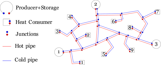
Figure 2: Sketch of a simplified DH system (c.f., [19]).

The tuning gains $k_{\mathrm{p},i}$ of the controllers (18) are all equal to $1\times 10^{-3}$. The same values are chosen for the gains $\kappa_{\mathrm{p},i}$ of the controllers $q_{\mathrm{p},i}$ in (20). This selection is based on a trial-and-error procedure aimed at attaining a fair balance between settling time and overshoot for the signals of interest. The producers’ and consumers’ temperature setpoints $T_{\mathrm{p},i}^{\star}$ and $T_{\mathrm{c},i}^{\star}$ are chosen to be equal to $85~{}^{\circ}\mathrm{C}$ and $55~{}^{\circ}\mathrm{C}$, respectively.

An explanation of the simulation results shown in Fig. 3 is as follows. The system is initialized in the vicinity of a system’s equilibrium in a context of low consumer demand (50% w.r.t. full demand) with $P_{\mathrm{c}}=(1.65,1.98,2.97,2.31,1.98,1.32,3.3,2.31,1.65)~{}$MW and with relatively small values for the storage tanks’ volumes setpoints with $V_{\mathrm{sh}}^{\star}=(100,150,200)~{}\mathrm{m}^{3}$. Convergence of the signals on display is observed after a short transient (states and inputs). At $t=6$h all storage tanks switch to a charging mode and attain their respective new setpoint $V_{\mathrm{sh}}^{\star}=(850,900,950)~{}\mathrm{m}^{3}$ at approximately $t=9$h. Note that the tanks switching to a charging mode causes an increase in the producers’ powers $P_{\mathrm{p},i}$ and flow $q_{\mathrm{p},i}$ during the process. At $t=12$h the consumers’ heat demands are simultaneously increased to higher values (75% w.r.t. full demand). The plot of some consumers’ flows $q_{{c},i}$ shows an increase at this instant and, after a short transient, the consumers’ temperatures return to their fixed setpoints. Observe that the increase in $P_{\mathrm{c},i}$ induces adjustments to the equilibrium values of $P_{\mathrm{p},i}$ and $q_{\mathrm{p},i}$ too, but without significant overshoots. At $t=18$h the tanks switch now to a discharging mode that ends at approximately $t=21$h. During this process, it is possible to see a reduction in producers’ powers and flows, contrary to what is observed during the tanks’ charging mode. The new, lower values for the entries of $V_{\mathrm{sh}}^{\star}$ are maintained until the end of the simulation. Finally, it is observed that the producers’ temperatures $T_{\mathrm{p},i}$ reach quickly (exponentially) their setpoints and remain at this value during the whole simulation time.

In order to test the effect of potential physical or practical constraints, we performed additional numerical simulations where we saturated the values of all the inputs $q_{\mathrm{p},i}$, $P_{\mathrm{p},i}$ and $q_{\mathrm{c},i}$ such that they are positive and upper bounded by maximum nominal values. In Fig. 4 we have simulated the same scenario as for the results in Fig. 3, considering additionally input constraints as described above. Note that, except for a slower charging rate for the hot layer of storage tank 2, there are no significant behavioral changes of the signals of interest with respect to those in Fig. 3. Various additional numerical experiments were conducted by taking random initial conditions with at most a 25% deviation with respect to a nominal equilibrium point and we obtained similar results (see Fig. 5).

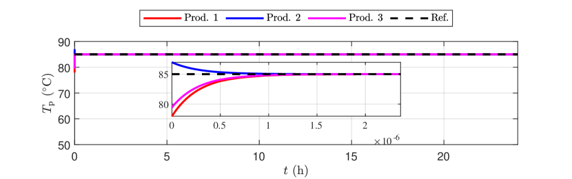
(a)  

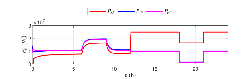
(b)  

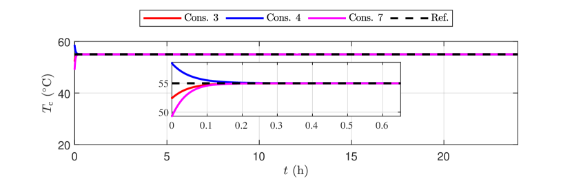
(c)  

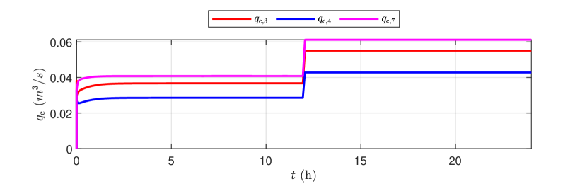
(d)  

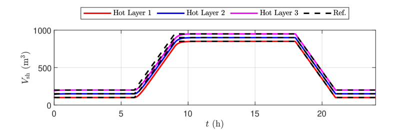
(e)  

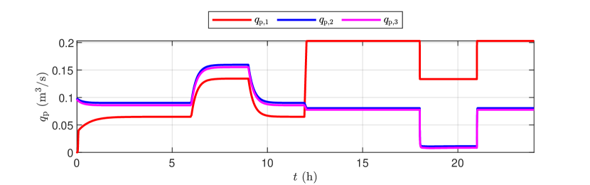
(f)  

Figure 3: Left column, top to bottom: evolution of the producers’ temperatures $T_{\mathrm{p},i}$, some of consumers’ outlet temperatures $T_{\mathrm{c},i}$ and the volume of hot water in the storage tanks $V_{\mathrm{sh},i}$. Right column, top to bottom: evolution of the inputs $P_{\mathrm{p},i}$, some of the inputs $q_{\mathrm{c},i}$, and the inputs $q_{\mathrm{p},i}$.

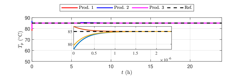
(a)  

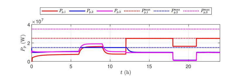
(b)  

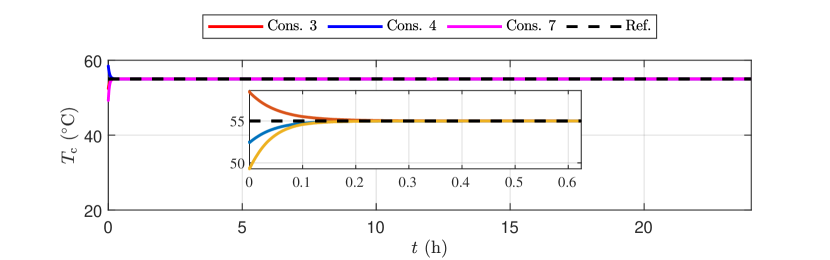
(c)  

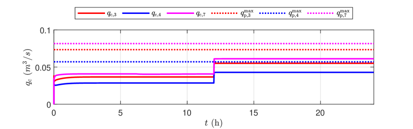
(d)  

(e)  

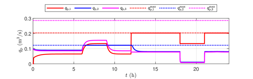
(f)  

Figure 4: Left column, top to bottom: evolution of the producers’ temperatures $T_{\mathrm{p},i}$, some of the consumers’ outlet temperatures $T_{\mathrm{c},i}$ and the volume of hot water in the storage tanks $V_{\mathrm{sh},i}$. Right column, top to bottom: evolution of the inputs $P_{\mathrm{p},i}$, some of the inputs $q_{\mathrm{c},i}$, and the inputs $q_{\mathrm{p},i}$. The scenario is the same as for the results in Fig. 3, but considering saturation to the control inputs.

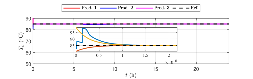
(a)  

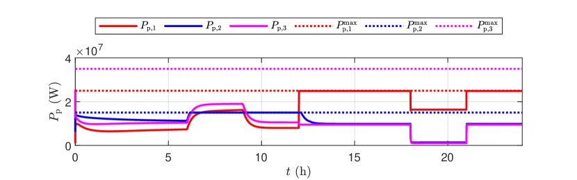
(b)  

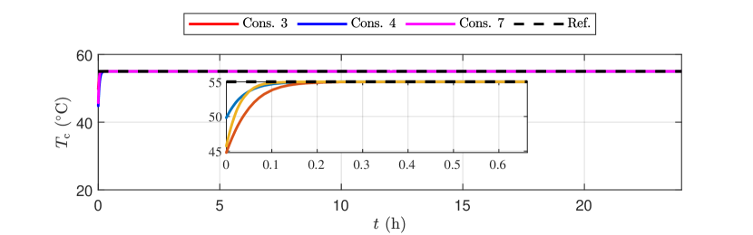
(c)  

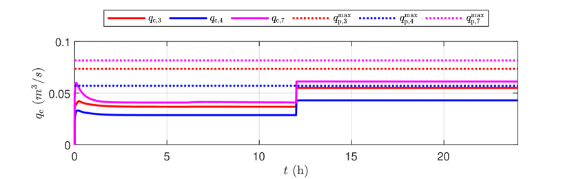
(d)  

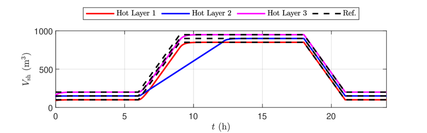
(e)  

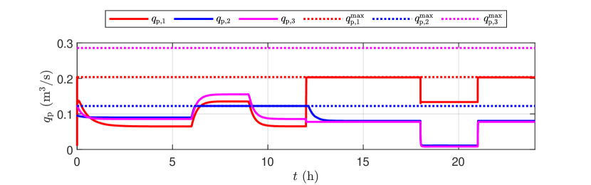
(f)  

Figure 5: Sample of additional numerical simulations we performed taking initial conditions that further deviate from a system equilibrium (up to 25% deviation) and considering input constraints. Left column, top to bottom: evolution of the producers’ temperatures $T_{\mathrm{p},i}$, some of consumers’ outlet temperatures $T_{\mathrm{c},i}$ and the volume of hot water in the storage tanks $V_{\mathrm{sh},i}$. Right column, top to bottom: evolution of the inputs $P_{\mathrm{p},i}$, some of the inputs $q_{\mathrm{c},i}$, and the inputs $q_{\mathrm{p},i}$.

V Concluding remarks

Done In this letter, we have addressed producer supply and consumer return temperature control in multi-producer DH systems through the design of novel decentralized controllers that also consider the regulation of the amount of hot water of multiple, distributed storage tanks. The design is complemented with a Lyapunov theory-based closed-loop stability analysis, from which convergence of the variables of interest is guaranteed. Extensions to this work we are currently investigating include: time-varying heat demand profiles (c.f., [9]); more detailed consumer models (c.f., [12]); fair energy distribution [4]; and input saturation [15].

References

- [1] H. Lund, S. Werner, R. Wiltshire, S. Svendsen, J. Thorsen, F. Hvelplund, and B. Mathiesen, “4th Generation District Heating (4GDH). Integrating smart thermal grids into future sustainable energy systems.” Energy, vol. 68, pp. 1–11, 2014.
- [2] E. Guelpa and V. Verda, “Thermal energy storage in district heating and cooling systems: A review,” Appl. Energy, vol. 252, 2019.
- [3] N. Novitsky, Z. Shalaginova, A. Alekseev, V. Tokarev, O. Grebneva, A. Lutsenko, O. Vanteeva, E. Mikhailovsky, R. Pop, P. Vorobev, et al., “Smarter smart district heating,” Proc. IEEE, vol. 108, no. 9, pp. 1596–1611, 2020.
- [4] A. Vandermeulen, B. van der Heijde, and L. Helsen, “Controlling district heating and cooling networks to unlock flexibility : A review,” Energy, vol. 151, pp. 103–115, 2018.
- [5] S. Buffa, M. H. Fouladfar, G. Franchini, I. Lozano Gabarre, and M. Andrés Chicote, “Advanced control and fault detection strategies for district heating and cooling systems—a review,” Appl. Sciences, vol. 11, no. 1, p. 455, 2021.
- [6] G. Sandou, S. Font, S. Tebbani, A. Hiret, and C. Mondon, “Predictive control of a complex district heating network,” Proc. 44th IEEE Conf. Decis. Control, and the European Control Conf., CDC-ECC ’05, vol. 2005, pp. 7372–7377, 2005.
- [7] R. Krug, V. Mehrmann, and M. Schmidt, “Nonlinear optimization of district heating networks,” Optim. Eng., vol. 22, no. 2, pp. 783–819, 2021.
- [8] F. Verrilli, S. Srinivasan, G. Gambino, M. Canelli, M. Himanka, C. Del Vecchio, M. Sasso, and L. Glielmo, “Model predictive control-based optimal operations of district heating system with thermal energy storage and flexible loads,” IEEE Trans. Autom. Sci. Eng., vol. 14, no. 2, pp. 547–557, 2016.
- [9] T. Scholten, C. De Persis, and P. Tesi, “Modeling and control of heat networks with storage: The single-producer multiple-consumer case,” IEEE Trans. Control Syst. Technol., vol. 25, no. 2, pp. 414–427, 2015.
- [10] J. Bendtsen, J. Val, C. Kallesøe, and M. Krstic, “Control of district heating system with flow-dependent delays,” IFAC-PapersOnLine, vol. 50, no. 1, pp. 13 612–13 617, 2017.
- [11] A. Krishna and J. Schiffer, “A port-hamiltonian approach to modeling and control of an electro-thermal microgrid,” IFAC-PapersOnLine, vol. 54, no. 19, pp. 287–293, 2021.
- [12] R. Alisic, P. E. Paré, and H. Sandberg, “Modeling and Stability of Prosumer Heat Networks,” IFAC-PapersOnLine, vol. 52, no. 20, pp. 235–240, 2019.
- [13] C. De Persis and C. Kallesøe, “Pressure regulation in nonlinear hydraulic networks by positive and quantized controls,” IEEE Trans. Control Syst. Technol., vol. 19, no. 6, pp. 1371–1383, 2011.
- [14] C. De Persis, T. Jensen, R. Ortega, and R. Wisniewski, “Output regulation of large-scale hydraulic networks,” IEEE Trans. Control Syst. Technol., vol. 22, no. 1, pp. 238–245, 2014.
- [15] T. Scholten, S. Trip, and C. De Persis, “Pressure regulation in large scale hydraulic networks with input constraints,” IFAC-PapersOnLine, vol. 50, no. 1, pp. 5367–5372, 2017.
- [16] J. E. Machado, M. Cucuzzella, N. Pronk, and J. M. A. Scherpen, “Adaptive control for flow and volume regulation in multi-producer district heating systems,” IEEE Control Syst. Lett., vol. 6, pp. 794–799, 2022.
- [17] S. Trip, T. Scholten, and C. De Persis, “Optimal regulation of flow networks with transient constraints,” Automatica, vol. 104, pp. 141–153, 2019.
- [18] J. E. Machado, M. Cucuzzella, and J. M. Scherpen, “Modeling and passivity properties of multi-producer district heating systems,” Automatica, vol. 142, 2022.
- [19] Y. Wang, S. You, H. Zhang, W. Zheng, X. Zheng, and Q. Miao, “Hydraulic performance optimization of meshed district heating network with multiple heat sources,” Energy, vol. 126, pp. 603–621, 2017.
- [20] S.-A. Hauschild, N. Marheineke, V. Mehrmann, J. Mohring, A. M. Badlyan, M. Rein, and M. Schmidt, “Port-hamiltonian modeling of district heating networks,” in Progress in Differential-Algebraic Equations II. Springer, 2020, pp. 333–355.
- [21] F. Strehle, J. Vieth, M. Pfeifer, and S. Hohmann, “Passivity-based stability analysis of hydraulic equilibria in 4th generation district heating networks,” IFAC-PapersOnLine, vol. 54, no. 19, pp. 261–266, 2021.
- [22] P. Vladimarsson, “District heat distribution networks,” in Short Course VI on Utilization of Low- and Medium-Enthalpy Geothermal Resources and Financial Aspects of Utilization. UNU-GTP and LaGeo, 2014.
- [23] L. Gentili, A. Paoli, and C. Bonivento, “Input disturbance suppression for port-Hamiltonian systems: An internal model approach,” Lect. Notes Control Inf. Sci., vol. 353, pp. 85–98, 2007.