BayesFormer: Transformer with Uncertainty Estimation

Abstract

Transformer has become ubiquitous due to its dominant performance in various NLP and image processing tasks. However, it lacks understanding of how to generate mathematically grounded uncertainty estimates for transformer architectures. Models equipped with such uncertainty estimates can typically improve predictive performance, make networks robust, avoid over-fitting and used as acquisition function in active learning. In this paper, we introduce BayesFormer, a Transformer model with dropouts designed by Bayesian theory. We proposed a new theoretical framework to extend the approximate variational inference-based dropout to Transformer-based architectures. Through extensive experiments, we validate the proposed architecture in four paradigms and show improvements across the board: language modeling and classification, long-sequence understanding, machine translation and acquisition function for active learning.

1 Introduction

Transformer-based architectures [58] are now the primary state-of-the-art (SOTA) models for a number of tasks in the computer vision [13], natural language processing [58] and speech recognition [11] domains. They have shown superior capabilities in a multitude of settings including classification, regression, time-series forecasting [36] and reinforcement learning [5]. For instance, within the natural language processing domain, the notion of large language models (LLM) such as BERT [9] and RoBERTa [38] have emerged which are pretrained on internet scale data and then used to perform few-shot learning by fine-tuning on target data labels. This paradigm has led to breakthrough results in sentiment analysis, text classification and question answering. Due to this superiority in predictive capabilities, transformers have started to be used as the primary modeling technique in a number of real-world machine learning systems.

Despite the progress made on improving the predictive capabilities of transformers, lesser attention has been devoted to understanding the quality of predictions on individual data. In particular, when integrating transformers into real-world systems a practitioner is concerned about details beyond average performance such as robustness, fairness, over-fitting and confidence of predictions. For example, Figure 1 depicts a LLM pretrained on 16GB of internet data (similar to BERT) and then finetuned on a paraphrase classification dataset (MRPC [10]) for the purpose of predicting whether a given sentence is a paraphrase or not. We see that the commonly used RoBERTa_base LLM [38] quickly overfits during finetuning. A primary aspect of understanding the quality of individual predictions is via uncertainty quantification. At its core, uncertainty quantification is concerned with the ability of models to output a notion of confidence of a prediction along with the prediction.

Uncertainty quantification for machine learning models is a rich-area of study (e.g., [31, 3, 39]). It is the key tool used to help a system convert a point-prediction to a reliable decision. Some applications include helping balance exploration-exploitation in recommendation systems [8], as acquisition functions in active learning [34], improving robustness on individual predictions [24], avoiding over-fitting on unseen datasets [17]. Seminal works have shown various methods to derive uncertainty estimates for feed-forward neural networks [16], recurrent neural networks such as LSTMs and GRUs [17] and Convolutional neural networks [15]. However, we have limited understanding of these techniques in the context of Transformers. There is only one recent work [19] that aims to use last-layer ensemble to obtain uncertainty estimates and apply it in the context of active learning.

In this work, we seek to scientifically understand how to provide uncertainty quantification on individual predictions of transformers that are mathematically grounded.

The main contribution of this paper is to use the approximate variational inference lens of dropout [16] applied to transformer architectures to derive the BayesFormer architecture. BayesFormer can be used to obtain interpretable uncertainty estimates on individual predictions and thus, help alleviate many of the issues mentioned above such as overfitting in small datasets. We provide the theory supporting BayesFormer and validate empirically by showing improved aggregate performance in a variety of paradigms including large language models’ pre-train-then-fine-tune applications, large-range context understanding problems, machine translation and active learning. The key architectural difference in BayesFormer is the application of dropout masks; both where and how they are applied. This is derived using approximate variational inference to compute the posterior distribution over the weights, given a finite dataset and the prior initialization distribution.

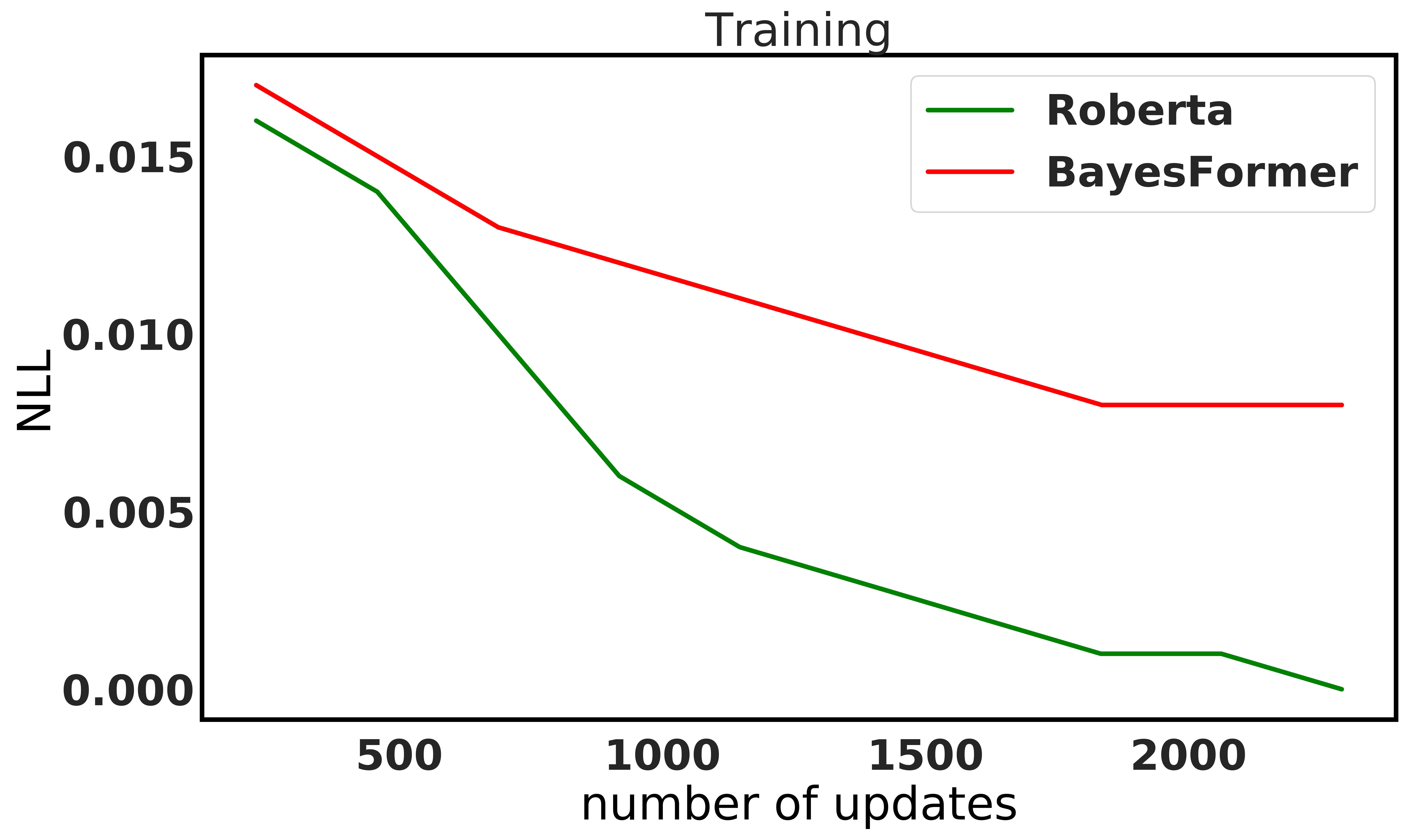
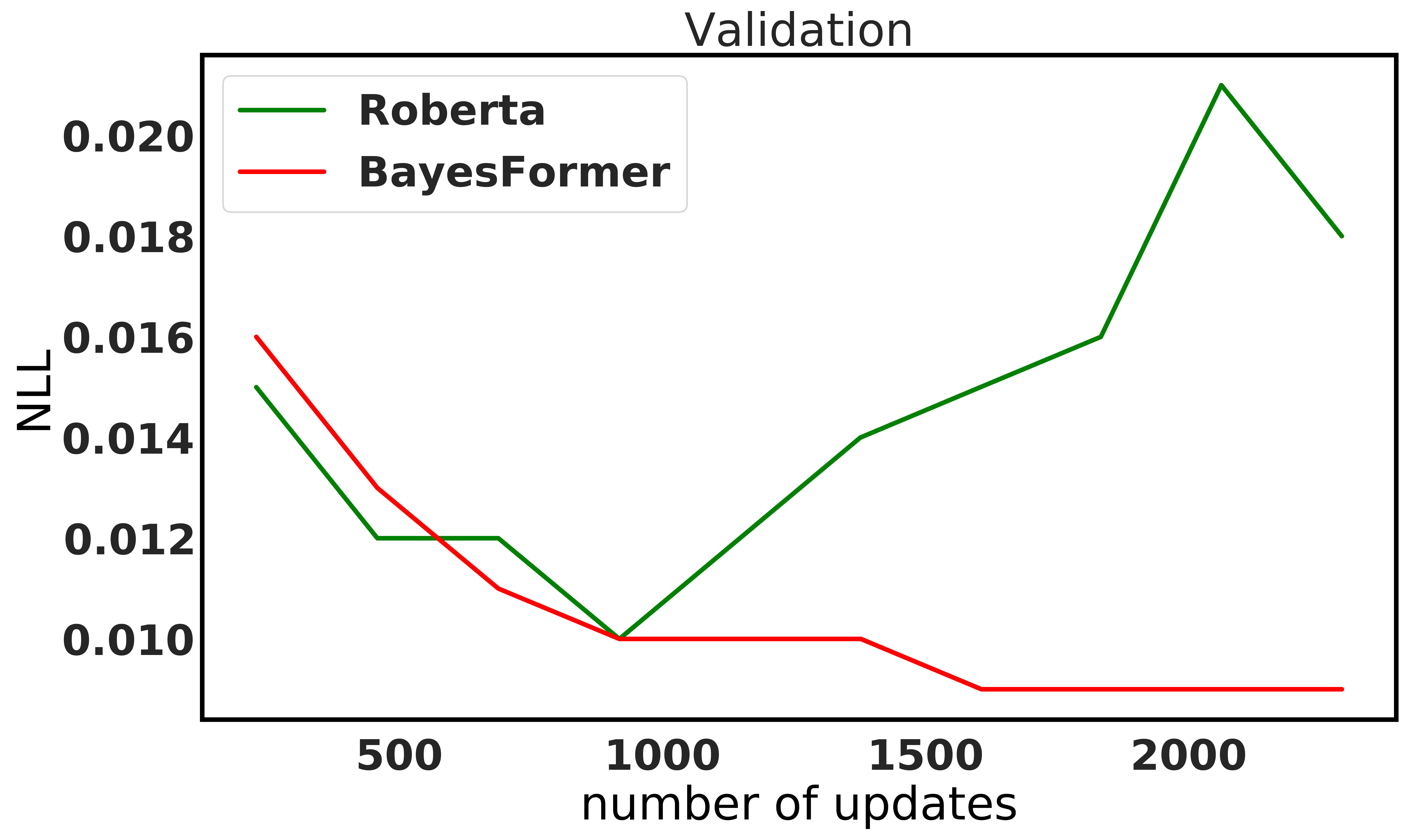
Figure 1: Negative log-likelihood evolution when fine-tuning LLM on MRPC dataset

2 Background

In this section we give the required background on approximate variational inference, Transformers and Bayesian neural networks.

2.1 Bayesian neural networks and approximate variational inference

The goal of approximate variational inference in connection to Bayesian neural networks is to characterize the posterior distribution of the network weights given the data and prior initialization. The typical prior distribution placed over the weights is $\mathcal{N}(0,\sigma^{2}\mathbf{I})$ for a small value $\sigma$. Denote $p(\mathbf{W}~{}|~{}\mathbf{X},\mathbf{Y})$ as the posterior distribution of the weights given the dataset $(\mathbf{X},\mathbf{Y})$. Equipped with an exact computation of this probability, one could then perform prediction on a new data point $\mathbf{x}$ using the formula

$$p(\mathbf{y}~{}|~{}\mathbf{x})=\int p(\mathbf{y}~{}|~{}\mathbf{x},\mathbf{W})\cdot p(\mathbf{W}~{}|~{}\mathbf{X},\mathbf{Y})\cdot d\mathbf{W}$$

However, the distribution $p(\mathbf{W}~{}|~{}\mathbf{X},\mathbf{Y})$ is extremely complex; we bypass by leveraging approximate variational inference (e.g., [16, 17, 20, 3]), where we approximate the distribution by a surrogate distribution $q(\mathbf{W})$ that is easier to compute and minimize the evidence lower bound $\mathtt{KL}(q(\mathbf{W})||p(\mathbf{W}~{}|~{}\mathbf{X},\mathbf{Y}))$ over all possible surrogates $q(.)$.

Thus, one needs to solve the following variational optimization problem

$$\min_{q}\mathtt{KL}(q(\mathbf{W})||p(\mathbf{W}~{}|~{}\mathbf{X},\mathbf{Y}))$$ (1)

It can be shown that this is equivalent to the following minimization program.

$$\min_{q}-\int q(\mathbf{W})\cdot\log[p(\mathbf{Y}~{}|~{}\mathbf{X},\mathbf{W})]\cdot d\mathbf{W}+\mathtt{KL}(q(\mathbf{W})||p(\mathbf{W}))$$ (2)

For a finite dataset $\{\mathbf{x}_{i},\mathbf{y}_{i}\}_{i=1}^{n}$ we use the empirical risk minimization framework to equivalently solve the following optimization problem.

$$\min_{q}-\sum_{i=1}^{n}\int q(\mathbf{W})\cdot\log[p(\mathbf{y}_{i}~{}|~{}\mathbf{x}_{i},\mathbf{W})]\cdot d\mathbf{W}+\mathtt{KL}(q(\mathbf{W})||p(\mathbf{W}))$$ (3)

2.2 Transformer Architecture

The key component of a transformer is the multi-head attention unit. Each head within this attention unit $a$ is parameterized by three matrices $\mathbf{W}_{Q,a}$, $\mathbf{W}_{K,a}$ and $\mathbf{W}_{V,a}$ corresponding to the query, key and value matrices $\mathbf{X}_{\mathtt{query}},\mathbf{X}_{\mathtt{key}},\mathbf{X}_{\mathtt{val}}\in\mathbb{R}^{n\times d}$ respectively. Here $n$ is the length of the input sequence and $d$ is the length of the embedding.

$$\mathbf{Z}_{a}(\mathbf{X})=\sigma\left(\frac{\mathbf{X}_{\mathtt{query}}\cdot\mathbf{W}_{Q,a}\cdot\mathbf{W}_{K,a}^{T}\cdot\mathbf{X}_{\mathtt{key}}^{T}}{\sqrt{d}}\right)\cdot\mathbf{W_{V,a}}\cdot\mathbf{X}_{\mathtt{val}}$$ (4)

In the typical usage of the attention unit, the so-called self-attention is used on the input, where $\mathbf{X}_{\mathtt{attn}}:=\mathbf{X}_{\mathtt{query}}=\mathbf{X}_{\mathtt{key}}=\mathbf{X}_{\mathtt{val}}$.

The Transfomer encoder architecture with self-attention is obtained as follows. Given an input $\mathbf{x}$ we obtain a sequence of positions $\mathbf{p}$. We learn an embedding $X_{\mathtt{input}}$ and $X_{\mathtt{pos}}$ by learning the corresponding weights $W_{\mathtt{input}}$ and $W_{\mathtt{pos}}$ and concatenating the outputs followed by a layer-norm to obtain $\mathbf{X}_{\mathtt{attn}}$. The architecture itself is then a stack of self-attention followed by a MLP block.

Of particular interest to the main results of this paper are the learnable weights $\mathbf{W}_{\mathtt{input}},\mathbf{W}_{\mathtt{pos}}$ the weights in the self-attention units $\mathbf{W}_{Q,a},\mathbf{W}_{K,a},\mathbf{W}_{V,a}$ and the weights in the MLP block $\mathbf{W}_{\mathtt{mlp}}$.

3 Variational Inference, Dropout and BayesFormer

In this section, we derive the new dropout procedure for transformers obtained by using approximate variational inference to find an approximate optimal solution $q(.)$ to the Equation (1).

We view each learnable parameter in the Transformer model as a random variable. For ease of notation, we merge the bias term (if any) into the corresponding weight matrix and the associated input vector. Additionally, for ease of presentation we consider the encoder only architecture of the Transformer. This can easily be extended to encoder-decoder transformer architectures.

For a given example $(\mathbf{X},\mathbf{y})$, let $\mathbf{f}_{\mathbf{y}}$ denote the output of the encoder architecture of the transformer model. To mathematically describe the transformer architecture we need to setup some notations. Let $\ell$ denote the number of multi-head attention layers and let $k$ denote the number of heads within each layer. Let $\mathbf{X}_{\mathtt{attn}}$ denote the input to the multi-head attention layers. Recall from subsection 2.2 $\mathbf{W}_{\mathtt{input}},\mathbf{W}_{\mathtt{pos}}$ denote the weights to learn an input embedding and the position embedding respectively. Thus $\mathbf{X}_{\mathtt{attn}}$ can be written as

$$\mathbf{X}_{\mathtt{attn}}:=\mathbf{X}_{\mathtt{input}}\cdot\mathbf{W}_{\mathtt{input}}\odot\mathbf{X}_{\mathtt{pos}}\cdot\mathbf{W}_{\mathtt{pos}}.$$ (5)

For layer $i$ and head $j$, we define $\mathbf{Z}_{i,j}(\mathbf{X}_{\mathtt{mha}})$ as the self-attention as defined in Equation (4). We combine the outputs of the $k$ heads at layer $i$ and define $\mathbf{Z}_{i}:=\mathbf{Z}_{i,1}\odot\mathbf{Z}_{i,2}\odot\ldots\odot\mathbf{Z}_{i,k}$. Let $\mathtt{LN}(.)$ denote the layer norm function and let $\mathbf{X}_{\ell,\mathtt{attn}}$ denote the input to layer $\ell$. Here the function $\sigma(.)$ is a pointwise operator applied on each entry of the matrix.

$$\mathbf{f}_{\mathbf{y}}(\mathbf{X}_{\mathtt{attn}})=\sigma(\mathbf{W}_{\mathtt{mlp},\ell}^{T}\cdot\mathtt{LN}(\mathbf{Z}_{\ell}(\sigma(\mathbf{W}_{\mathtt{mlp},\ell-1}^{T}\cdot\mathtt{LN}(\mathbf{Z}_{\ell-1}(\ldots\mathbf{X}_{\mathtt{attn}})\ldots)+\mathbf{X}_{\ell,\mathtt{attn}}))$$ (6)

Let $\mathbf{W}$ denote the set of random matrices corresponding to the learnable parameters

$$\{\{\mathbf{W}_{\mathtt{mlp},i}\}_{i=1}^{\ell},\{\mathbf{W}_{Q,i,j},\mathbf{W}_{K,i,j},\mathbf{W}_{V,i,j}\}_{i=1,j=1}^{i=\ell,j=k}\}$$

with the prior distribution being the standard normal distribution independent across the matrices and entries within the matrix. Let $\mathbf{f}_{\mathbf{y},\mathbf{W}}(\mathbf{X})$ denote the corresponding model output on input $\mathbf{X}$. Let $\mathcal{D}=\{\mathbf{y}_{i},\mathbf{X}_{i}\}_{i=1}^{n}$ denote the finite dataset at hand. Consider the ERM approximation in Equation (3). For each term $i$ in the summation, we consider the integral

$$\int q(\mathbf{W})\cdot\log[p(\mathbf{y}_{i}~{}|~{}\mathbf{f}_{\mathbf{y}_{i},\mathbf{W}}(\mathbf{X}_{i}))]\cdot d\mathbf{W}$$

Similar to [16], we can approximate the above integral by noting that it computes the expectation of the quantity $\log[p(\mathbf{y}_{i}~{}|~{}\mathbf{f}_{\mathbf{y}_{i},\mathbf{W}}(\mathbf{X}_{i}))]$ over $\mathbf{W}$ that follows the distribution $q(\mathbf{W})$. Thus, we can obtain a unbiased estimate $\widehat{\mathbf{W}}_{i}\sim q(\mathbf{W})$ and approximate the integral by,

$$\int q(\mathbf{W})\cdot\log[p(\mathbf{y}_{i}~{}|~{}\mathbf{f}_{\mathbf{y}_{i},\mathbf{W}}(\mathbf{X}_{i}))]\cdot d\mathbf{W}\approx\log[p(\mathbf{y}_{i}~{}|~{}\mathbf{f}_{\mathbf{y}_{i},\widehat{\mathbf{W}}_{i}}(\mathbf{X}_{i}))]$$

Computing $n$ i.i.d. samples $\widehat{\mathbf{W}}_{1},\widehat{\mathbf{W}}_{2},\ldots,\widehat{\mathbf{W}}_{n}\sim q(\mathbf{W})$ and plugging it back into Equation (3) we get the optimization function to be approximately,

$$\min_{q}-\sum_{i=1}^{n}\log[p(\mathbf{y}_{i}~{}|~{}\mathbf{f}_{\mathbf{y}_{i},\widehat{\mathbf{W}}_{i}}(\mathbf{X}_{i}))]+\mathtt{KL}(q(\mathbf{W})||p(\mathbf{W}))$$ (7)

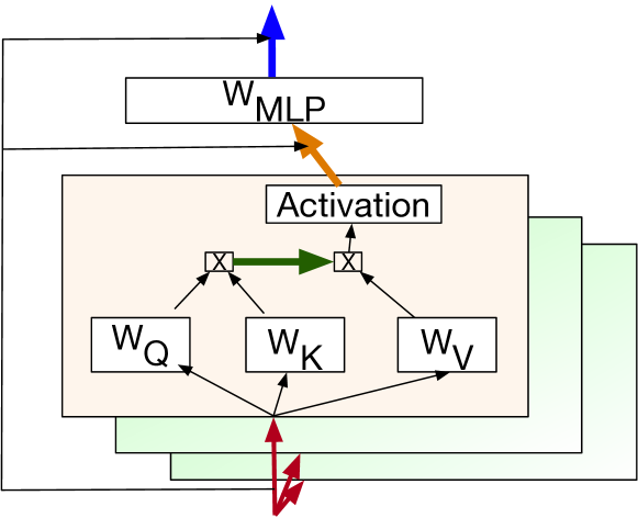
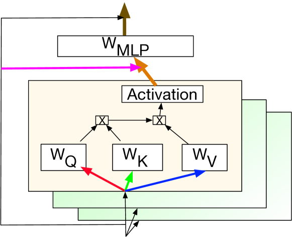
Figure 2: (left) Dropout application in the standard transformer architecture (right) Proposed dropout application derived from approximate variational inference. Same colored arrows indicate the same random outcomes while different colors indicate independent random variables.

To solve the optimization problem in equation (7), we need to provide two details: (a) to solve the minimization problem over a reasonable class of functions $q(.)$. (b) for any given function $q(.)$, the ability to compute an unbiased estimate $\widehat{\mathbf{W}}$.

3.1 Variational distribution $q(.)$

Following the prior works on ANN [16] and RNN [17], we define the family of variational distributions $q(.)$ for each matrix in $\mathbf{W}_{*}$ parametrized by $\mathbf{M}_{*}$. For ease of notation, we denote this family by $q_{\mathbf{M}}(.)$. Let $\mathbf{W}_{*,i},\mathbf{M}_{*,i}$ refer to any given row $i$ in matrices $\mathbf{W}_{*}$ and $\mathbf{M}_{*}$ respectively. The distribution $q_{\mathbf{M}}(\mathbf{W})$ is defined as follows. For each $\mathbf{W}_{\ast}\in\mathbf{W}$ can be defined as,

$$\mathbf{W}_{{\ast},i}\sim p\mathcal{N}(0,\sigma^{2}\mathbf{I})+(1-p)\mathcal{N}(\mathbf{M}_{*,i},\sigma^{2}\mathbf{I}).$$ (8)

In equation (8), the quantity $p$ represents the apriori defined probability and $\sigma$ is the quantity used in the prior initialization of the weights.

Plugging this variational distribution $q_{\mathbf{M}}(.)$ back in the optimization problem in equation (7), we get

$$\min_{q_{\mathbf{M}}}-\sum_{i=1}^{n}\log[p(\mathbf{y}_{i}~{}|~{}\mathbf{f}_{\mathbf{y}_{i},\widehat{\mathbf{W}}_{i}}(\mathbf{X}_{i}))]+\mathtt{KL}(q_{\mathbf{M}}(\mathbf{W})||p(\mathbf{W}))$$ (9)

As shown in [16], when the prior distribution $p(\mathbf{W})$ are all initialized using the standard normal distribution, we obtain the standard loss maximum likelihood loss function with $\ell_{2}$ regularization over the weight matrices. In particular, the first term minimizes the negative log-likelihood, while the KL(..) term for the above variational distribution family $q(.)$ (approximately) reduces to minimizing the square of the $\ell_{2}$-norm of $\mathbf{M}$ when the prior distribution $p(\mathbf{W})$ is the standard normal distribution. Thus, for this definition of $q(.)$, the optimal solution to the approximate variational inference evidence lower bound is equivalent to the standard trasnformer training objective.

3.2 BayesFormer and obainting unbiased estimate $\widehat{\mathbf{W}}$

Given the above variational distribution $q(.)$ we now provide details on obtaining an unbiased estimate $\widehat{\mathbf{W}}$. To do this, we introduce the BayesFormer archietecture which modifies the application of dropout to the standard transformer architecture. We then obtain the following theorem.

Theorem 1.

For any input $\mathbf{X}$, we have the following properties of the BayesFormer architecture.

1. Computing the model output $\mathbf{f}_{\mathbf{y},\widehat{\mathbf{W}}}(\mathbf{X})$ is equivalent to performing a forward pass on the input $\mathbf{X}$ and applying the dropout with probability $p$ in the BayesFormer architecture.

2. The posterior $p(\mathbf{y}~{}|~{}\mathbf{X})\approx\frac{1}{T}\sum_{t=1}^{T}\mathbf{f}_{\mathbf{y},\widehat{\mathbf{W}}_{t}}(\mathbf{X})$ where $\mathbf{f}_{\mathbf{y},\widehat{\mathbf{W}}_{t}}(\mathbf{X})$ is the output of the $t^{th}$ forward pass through the BayesFormer architecture. Moreover, the predictive uncertainty over the prediction $p(\mathbf{y}^{*}~{}|~{}\mathbf{X}^{*})$ can be approximated by the empirical lower and upper confidence intervals of the $T$ forward passes.

In the rest of this subsection, we prove Theorem 1 by describing the BayesFormer architecture. From the definition of the variational distribution in equation (9) we have that each row of each of the weight matrix is zeroed out with probability $p$. Motivated by this, in BayesFormer we independently apply dropout mask to the vectors $\mathbf{X}_{\mathtt{input}}$ and $\mathbf{X}_{\mathtt{pos}}$. This would amount to independently dropping the rows of the matrices $\mathbf{W}_{\mathtt{input}}$ and $\mathbf{W}_{\mathtt{pos}}$. In a typical input to a transformer this corresponds to the input sequence (e.g., a sentence) and is commonly not regularized. The dropout mask is applied after the corresponding input and position embedding is computed. However, in BayesFormer architecture we apply the dropout masks before the embedding is computed. This ensures that these embeddings themselves aren’t suffering from overfitting and the model is forced to not depend on any single input in the sequence.

Next, in BayesFormer we modify the application of dropout in the self-attention unit. First, the dropout mask for each layer $i\in\ell$ and each head $j\in k$ is chosen independently. Second, for a self-attention unit $i\in\ell$ and a head $j\in k$, combining equations (4) and (8) we apply dropout masks $h_{\mathtt{key}}$, $h_{\mathtt{query}}$ and $h_{\mathtt{val}}$ to the vectors $\mathbf{X}_{\mathtt{key}}$, $\mathbf{X}_{\mathtt{query}}$ and $\mathbf{X}_{\mathtt{val}}$ respectively. Note that in a typical self-attention unit the vectors $\mathbf{X}_{\mathtt{key}}$, $\mathbf{X}_{\mathtt{query}}$ and $\mathbf{X}_{\mathtt{val}}$ are identical yet in BayesFormer we sample three independent dropout masks and apply them separately to the vectors. This can be interpreted as projecting the self-attention matrices to random low-dimensional subspaces similar to that of efficient transformer architectures such as linformer [60]. Third, we do not apply any other dropout within the self-attention, notably removing the dropout that is typically applied before multiplying with $\mathbf{W}_{\mathtt{val}}$. This is not surprising, since we have already regularized by applying an independent dropout mask $h_{\mathtt{val}}$.

Finally, in BayesFormer we apply dropout mask to the input of the feed-forward layer following the multi-head self-attention. This input consists of two parts: concatenated output from the multi-head self-attention followed by a layer norm and a skip-connection that is the input to the multi-head self-attention of the previous layer. We apply a dropout mask $h_{\mathtt{mlp}}$ to this concatenated string before passing it through the feed-forward layer. As in the standard transformer architecture, the dropout application within the feed-forward layer remains unchanged. Figure 2 summarizes the key changes in BayesFormer compared to a standard transfomer architecture. In this figure, same color represents that the outcomes of random variable is shared, while different colors indicate independence in the outcomes.

Given the BayesFormer architecture, the proof of theorem 1 follows from equations (8) and (4).

4 Experiments

In this section, we summarize the results from the empirical evaluation of the proposed theory. We use four different paradigms that comprehensively illustrates the behavior of the proposed methods. We use language classification tasks, long range sequence understanding tasks, machine translation and active learning. We also explore how this dropout methodology integrates into other efficient transformer architectures (commonly referred to as x-formers). In all the conducted experiments, we control for as many sources of confounding variables as possible between the control and the test arms. This includes non-dropout related hyper-parameters, number of GPUs and/or nodes in distributed training and the seed used in random function invocation during data pre-processing. This helps us understand the contribution of the dropout variable independent of other architectural choices and thus, can be extended to other SOTA architectures when appropriate. Regarding the dropout hyper-parameters themselves, we tune the dropout probability in the small range of $\{0.05,0.1,0.2\}$ using a validation set for the task. Where resources are not specified a run of an experiment was performed using a single Nvidia A100 GPU on a single node of a cluster.

4.1 Pretrain and finetune paradigm for language classification tasks

The most salient application of the transformer architecture in natural language processing is to pretrain large language models (LLMs). LLMs are pretrained on internet scaled corpus using the masked language modelling approach to understand text. They are then used in language classification tasks such as sentiment analysis by finetuning the LLM on the small dataset corresponding to the task. Some common examples of LLMs include BERT [9], RoBERTa [38] which have had significant impact in the last few years.

Typically, finetuning on a target task leads to the potential of over-fitting since the number of labels available are small (compared to pretraining). The ability to perform large number of updates on the target dataset without over-fitting is crucial since it leads to improved performance. However, there is a trade-off between increasing the number of updates and the potential to over-fit and thus, early stopping is commonly employed ([38]).

In this experiment, we pretrain RoBERTa_base and our proposed model BayesFormer on the English wikipedia corpus appended with the Bookcorpus [66] totalling a size of 16GB. As described in [9], this corpus was used to pretrain the BERT model. For both the models we use the same hyper-parameters as used in [38]. For BayesFormer, all new dropout units use the dropout probability of 0.1. Both models are pre-trained for 250k steps.

We fine-tune the pretrained models on eight target datasets available in the GLUE dataset [59]. The tasks are acceptability (CoLA [61]), sentiment classification (SST2 [53]), paraphrase (MRPC [10], QQP [6]), sentence similarity (STS-B [4]) and natural language inference (MNLI [62], QNLI [48], RTE [2]). For finetuning, we use the same procedure as that of [38] where we tune the maximum learning rate $\in\{1e-5,2e-5,3e-5\}$, the batch size $\in\{16,32\}$ hyper-parameters for 10 epochs. We use the best checkpoint in the 10 epochs based on the performance on the validation set to evaluate on the dev set. The pretrained models were trained using distributed training on 8 nodes with each node containing 8 Nvidia A100 GPUs. The finetuning runs on the other hand were run on a single Nvidia A100 GPU. We used the fairseq [45] code-base to implement the baselines, our method and run the data pre-processing and testing scripts.

Results and discussion. Table 1 summarizes the results of this experiment. As we can see, BayesFormer performs well on average and improves over RoBERTa_base on 6 out of the 8 GLUE tasks, comparably on one and performs worse on the other. To further explore the behavior of BayesFormer, we looked into the negative log-likelihood (nll) and the loss evolution during the 10 epochs of fine-tuneing. Figure 1 show that RoBERTa_base model very quickly over-fits (starting epoch 3) while BayesFormer does not overfit; both loss and nll continue to decrease with the number of updates.

Further ablations. We consider further ablation to understand the effect of datasize towards overfitting and thus, the eventual improvement in performance. We pretrain using only the English wikipedia dataset for pretraining the LLMs. Thus, the dataset size for pretraining is significantly smaller. We notice that the relative improvement of BayesFormer over RoBERTa_base in downstream GLUE tasks is higher when pretrained with the smaller English wikipedia corpus. Table 5 summarizes the results when trained with the smaller dataset. This further supports the fact that BayesFormer is less prone to overfitting compared to that of vanilla transformer.

Model	CoLA	SST2	MRPC	STSB	QQP	MNLI m/mm	QNLI	RTE	Avg
	(MCC)	(Acc)	(F1)	(P/S)	(F1/Acc)	(Acc)	(Acc)	(Acc)
RoBERTabase	62.1	94	90.9	87.3/87.3	88.5/91.5	84.9/84.9	91.4	74.7	84.6
BayesFormer	63.3	93.7	92.1	87.7/87.7	88.4/91.5	85.3/85.3	91.7	74.8	85

Table 1: Dev set results (median of five runs). RoBERTa_base v/s BayesFormer: pretrained on BERT corpus and finetuned on the GLUE benchmark datasets.

4.2 Long-range sequence understanding

Transformers are useful over prior architectures (e.g., LSTM) for sequential understanding problems since they are able to effectively learn long range contextual dependencies in data effectively. Recently, Long-range arena dataset [56] was introduced to provide a standardized evaluation of transformers in the long-context understanding setting. It contains five tasks across domains: Listops [43], byte-level text classification [26], byte-level document retrieval [21], Image classification on pixels [30] and Pathfinder [28]. The LRA repository provides scripts for data preprocessing, configs for parameters and an apples-to-apples comparison environment. We include our proposed approach to the softmax attention implementation and use the same configuration values. We set the dropout probability of new dropout operations at 0.05.

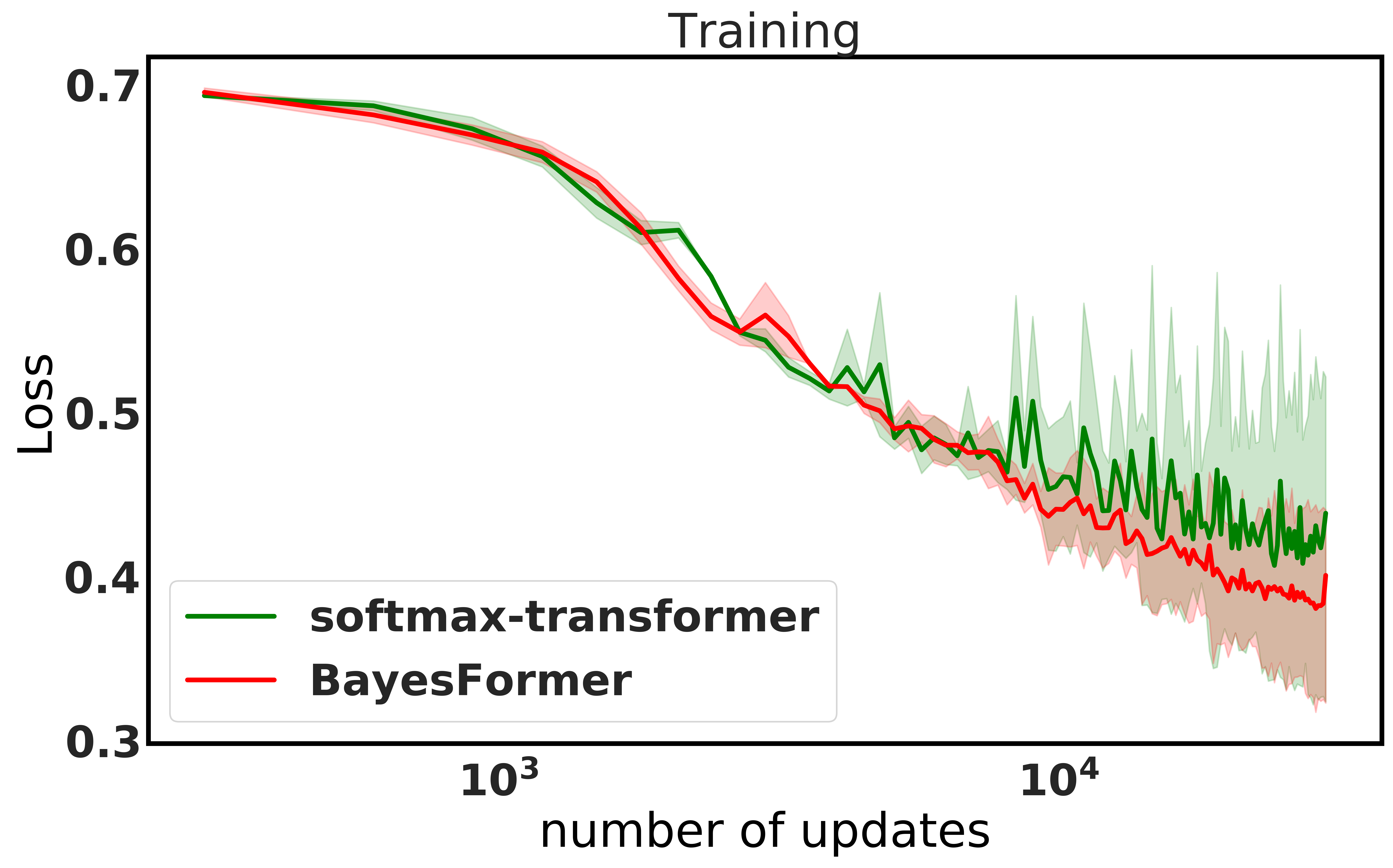
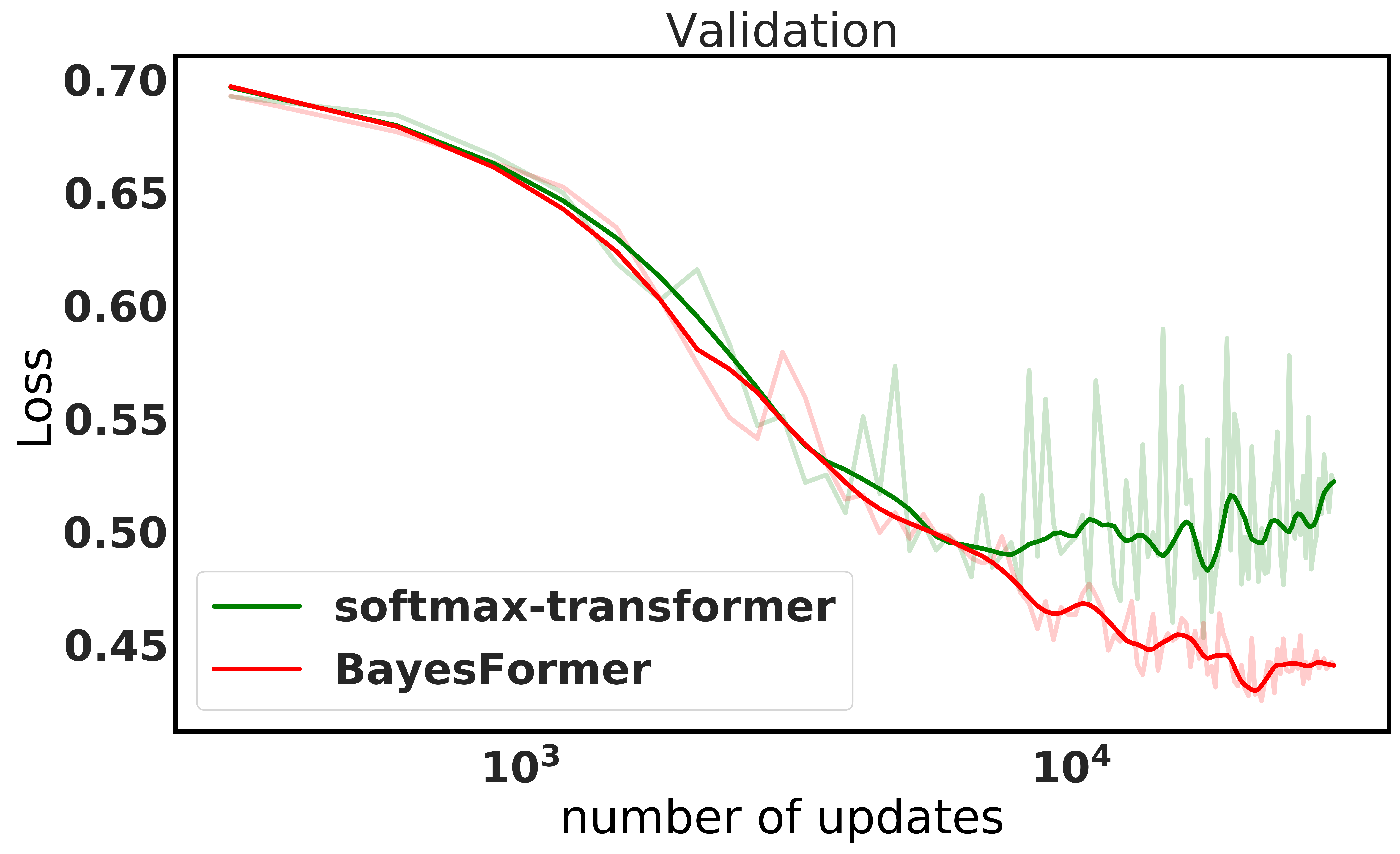
Figure 3: Loss v/s num. of updates on LRA retrieval dataset. Smoothed using lowess.

Model	Test accu.
Linear attention	17 (0.53)
BayesFormer - linear	19.1 (0.48)
Linformer	36.2 (0.17)
BayesFormer - linformer	36.6 (0.05)
Reformer	18 (0.78)
BayesFormer - reformer	18.1 (2.06)
Performer	19.4 (4.4)
BayesFormer - performer	23.4 (5.4)
Nystrom attention	34.6 (8.7)
BayesFormer - Nystrom	35.0 (0.75)

Table 2: Bayes dropout on various x-former attentions.

Results and discussion. Table 3 summarizes the results on the five LRA tasks. The results are median of five different runs. As we can see we consistently improve over the vanilla transformer showcasing the power of BayesFormer. We attribute these improvements to the ability to reduce over-fitting. To validate this, we plot the train and validation losses on the retrieval task as shown in Figure 3. We see that the softmax attention transformer start to overfit, as seen by the increasing validation loss with number of updates beyond a point, while the loss further continues to decrease in the validation set for BayesFormer. Surprisingly, we find that BayesFormer also is able to fit the training set better than vanilla transformer. This indicates that the new dropout method is also allowing for the transformer to connect contextual information in the input to a longer part of the sequence likely because the dropout forces the network to not rely on any single part of the input. Unlike the regular transformer, BayesFormer needs to depend on a lossy version of the key, query and value vectors while performing self-attention.

Further ablations. We further use the Listops dataset to evaluate the application of the new dropout on xformers to understand if this methodology is compatible with efficient transformer architectures. For each xformer, we use the base attention module that uses the dropout as described in the respective paper and compare against the dropout application as described by the above theory before and after the attention units. In particular, we do not modify the way dropout is applied within the attention units and treat all operations within the attention unit as a black-box. We consider linear attention [27], linformer [60], reformer [29], performer [7] and Nystrom attention [64] variants for the transformer architecture. All experiments were run using the code released by the Nystromformer paper authors.

Initial evidence indicates that the theoretically grounded version of dropout proposed in this paper can indeed improve architectures beyond those it was derived for. Thus, we recommend future SOTA models to test this methodology of dropout to improve the performance. Table 2 summarizes the results which is a median taken over 5 random runs.

Model	Listops	Image	Text	Retrieval	Pathfinder	Avg.
Transformer	36 (0.3)	38.6 (0.6)	64.8 (0.4)	78.4 (0.7)	69.8 (0.5)	57.5
BayesFormer	36.1 (0.4)	39.3 (0.6)	65.7 (0.2)	80.8 (0.1)	72.8 (0.5)	58.9

Table 3: Test set results (median of five runs) on LRA tasks.

4.3 Machine Translation

Machine translation is another important task in Natural language processing where the goal is to translate sentences in a source language to a sentence in the target language that preserves the meaning. This can naturally be modelled as a sequence-to-sequence task and transformer is typically used to achive SOTA results. To evaluate BayesFormer, we consider the IWSLT ’14 German to English translation task available in the fairseq repository [45]. We use the same scripts for preprocessing the data into train, validation and test splits. The dataset contains 160239 train examples, 7283 validation examples and 6750 test sentences.

Model	Val BLEU	Test BLEU
Transformer	35 (0.1)	34.5 (0.1)
BayesFormer	35.5 (0.1)	34.8 (0.1)

Table 4: IWSLT ’14 de $\rightarrow$ en test BLEU scores

We use the architecture transformer_iwslt_de_en available in fairseq repository as the baseline model and apply the proposed dropout methodology to this model. The number of parameters in this model is 34.5M. We do not modify any hyper-parameter apart from the dropout probability on the newly added dropout module which is set to 0.05. Thus, we do not change the dropout probabilities of those that are common to both the baseline and BayesFormer. Both the models are trained for 500k steps and the best checkpoint, as measured by the validation set BLEU score, is used to obtain BLEU scores on the test set. We apply label smoothing and use the LabelSmoothedCrossEntropyCriterion to train the model.

Results. Table 4 summarizes the BLEU score [46] on both the validation set and the test set. BayesFormer achieves a higher validation BLEU and consequently a higher test BLEU score over the baseline transformer variant.

4.4 Active learning

Active learning aims to smartly label a limited pool of samples that improves the classifier performance. Labelled data is typically costly to acquire and thus, active learning methods help with cutting down total labelled data needed for comparable performance [50]. Here we consider the pool-based setup where we can access any subset of data to obtain labels. Typical works (e.g.,  [51, 12]) in active learning consider the multi-round setting, where the active learning algorithm can obtain labels for a partial subset of data, retrain the classifiers and use that to acquire more data. However, these schemes are highly impractical for real-world systems. In most real-world systems, retraining classifiers is as costly, if not more, as obtaining the labels themselves. Hence, here we instead consider the harder single-round protocol of active learning where the sampling algorithm assigns scores to all the unlabelled data at once, and then labels are collected for the top-k data points based on this score.

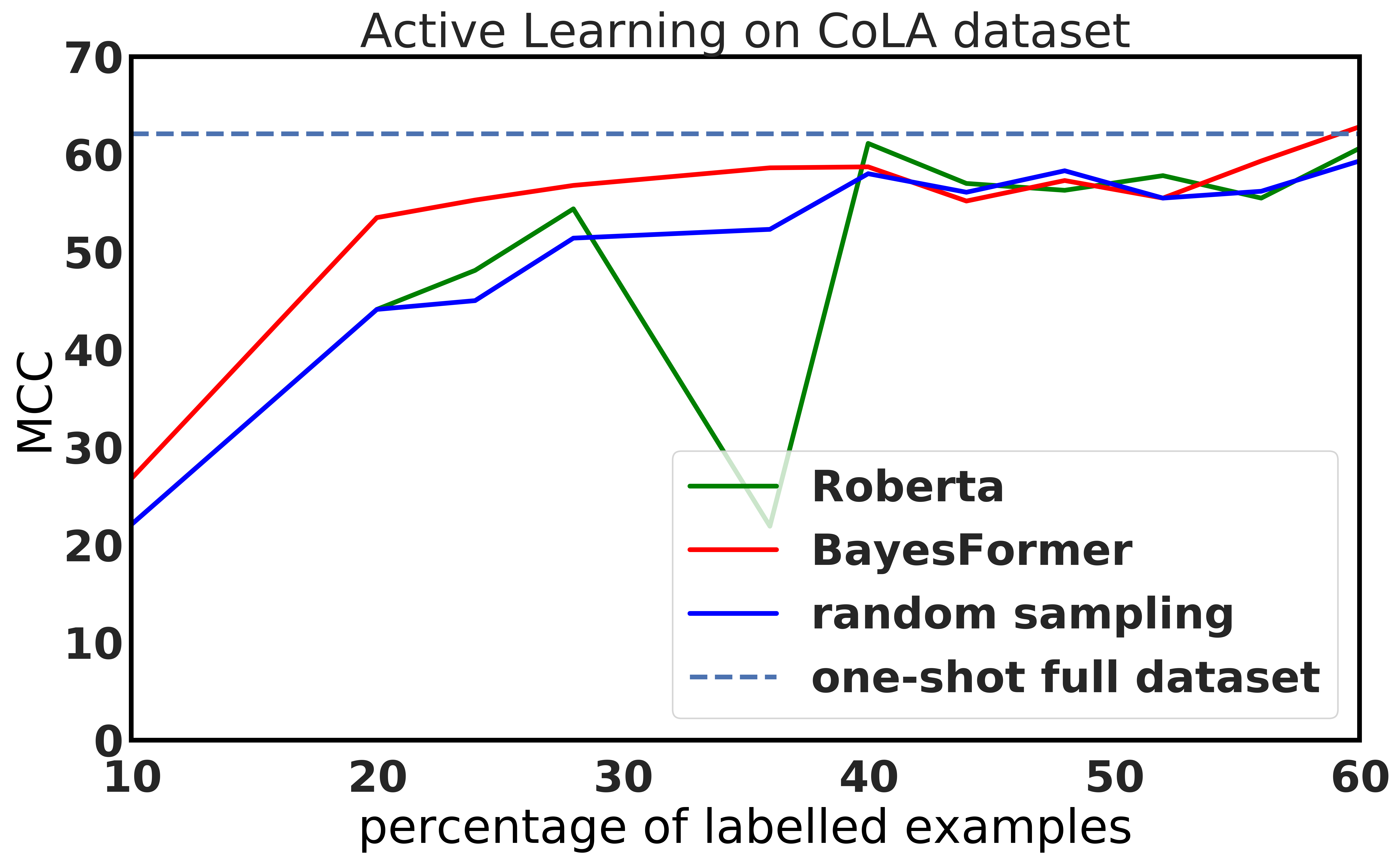
Figure 4: Active sampling during finetuning on CoLA dataset starting from the same pretrained checkpoint.

To test the effectiveness of the uncertainty estimates produced by the BayesFormer, we use the MCDropout [16] based BALD [18, 25] acquisition function (called MC-BALD) and compare it against two baselines: MC-BALD applied to the vanilla transformer model and random-sampling. The same pretrainined checkpoint of RoBERTa model is used as a starting point and active sampling is used to select examples for finetuning. We reuse the CoLA dataset from subsection 4.1. We warmstart by first finetuning the checkpoint on 10% of randomly chosen sentences. To obtain the MC-BALD scores for BayesFormer and RoBERTa, we perform 11 forward passes on each point. The remaining 90% of the CoLA dataset is scored using the three different strategies (i.e., MC-BALD for BayesFormer, RoBERTa and random score). We then finetune by choosing top-k based on these scores, for various values of $k$. Figure 4 shows the dev set MCC of the models, based on the percentage of labelled data used. We see that when the labelling budget is low, BayesFormer has a significantly higher MCC (by > 4 points) compared to RoBERTa and random sampling. And as the budget increases, the accuracy of all the three methods catch up as expected. This indicates that the estimates obtained by BayesFormer are more reliable compared to vanilla MCDropout application. A surprising side-effect of this experiment was that sometimes its better to throw away some labels to improve the dev set accuracy. Indeed, the best MCC for BayesFormer was 62.8 which outperformed the MCC of 59.6 obtained when trained on all data.

Model	CoLA (MCC)	SST2 (Acc)	MRPC (F1)	STSB (P/S)	MNLI m/mm (Acc)	QNLI (Acc)	RTE (Acc)
RoBERTabase	21.3	91.3	89.5	84.45/84.22	82.1/82.1	89.9	59.2
BayesFormer	32.1	91.5	90.9	85.58/85.26	83.3/83.3	91.3	65

Table 5: Dev set results (median of five runs). RoBERTa_base v/s BayesFormer: pretrained on English wikipedia corpus (small) and finetuned on the GLUE benchmark datasets.

5 Conclusion

In this paper, we extend the approximate variational inference lens of dropout to Transformer architectures. This helped us derive a new dropout structure with mathematical grounding. We verified the theory empirically on a wide variety of tasks. Based on the results of this paper, we suggest a few future directions. First, it would be interesting to understand the interplay of this dropout method with other techniques used to reduce over-fitting. In this paper, we briefly allude to it through ablation on dataset size, but we believe more work is needed. Second, we are also excited to understand its effect on other applications of large transformer models such as zero/few-shot learning and text generation. Third, we would like to understand model robustness and brittleness to adversarial examples for BayesFormer.

6 Acknowledgements

KAS is grateful to Darsh Shah for helping setup the fairseq environment.

Appendix A Appendix

Appendix B Extended Related Work

Our work falls at the intersection of Sequential decision making and Transformers. As such these areas of study are extensively explored independently.

Uncertainty estimates in sequential decision making. Uncertainty quantification can be primarily motivated in the context of sequential decision making, and in particular, the field of multi-armed bandits [52]. As illustrated in [16], neural networks with uncertainty estimates can be used to perform reinforcement learning [55]. They explore the Thompson sampling algorithm [49] and show that it outperforms the popular $\epsilon$-greedy algorithm [32]. Multi-armed bandits are the primary choice of techniques used for exploration in recommender systems [32, 35] due to its simplicity and effectiveness. Beyond recommender systems uncertainty based exploration is used in other applications such as advertising [1] and ride-share platforms [22]. Beyond multi-armed bandits, uncertainty estimates are also used for reinforcement learning algorithms such as [44, 40].

The other salient application of uncertainty in sequential decision making is in active learning [50]. Many classical active learning algorithms such as uncertainty sampling [33], Query-by-committee [41] and more recent ensemble approaches such as MCDropout [16], BALD [18], Bayes-by-backprop [3] and MAAL [14] all rely on either implicit or explicit uncertainty quantification of predictions of the current model to acquire the next batch of data.

Transformers. Following the initial breakthrough work of [58], Tranformer architectures have received a ton of attention. Some directions include efficient transformers [57] where the goal is to reduce the complexity of the costly self-attention computation while keeping the performance near parity. The survey above covers most of the innovations in this direction including benchmarks, models and applications. On the application side, transformer architecture has been used in computer vision [23], graphs [42] and natural language processing [37]. Recently, transformer architectures have also started to be deployed in practice [54, 47]. Tangentially related to our work is that of [63] where they explore many different positions dropout could be applied in a transformer architecture. Similar to our work, they notice the presence of over-fitting. However, different from our work, none of their dropout methods include the ones proposed in this paper. Another work that on the surface is related to our work is [65]. In this work, the authors propose to use MCDropout naively on existing application of dropout in the context of speech recognition. First, as we show in this paper for us to have formal guarantees on the posterior, we would need to modify the way dropout is applied. In that respect, the prior work is not truly Bayesian. Second, the goals of the two papers are different. Indeed, they are interested in improving speech recognition benchmarks, while we are interested in principled understanding irrespective of the application domain.

Appendix C Reproducibility details for experiments

In this section we specify how we chose the hyper-parameters for the baseline as well as BayesFormer in the various experiments.

Pretraining. For the pretraining of RoBERTa_base model, we used the same settings from [38]. For BayesFormer, we also chose the same set of hyper-paramters and settings. We did not do any hyper-paramter tuning at this step.

Finetuning. For finetuning on the various GLUE tasks, for both RoBERTa_base and Bayesformer, we tuned three hyper-parameters. Learning rate $\in\{1e-5,2e-5,3e-5,4e-5,5e-5,1e-4\}$, batch size in $\in\{16,32\}$ and the dropout probability $\in\{0.05,0.1,0.2\}$. We choose the best model based on the validation set metric.

LRA tasks. For LRA tasks, we did not change any hyper-parameter or settings. We cloned the code made available by authors of [64] and implemented our algorithm in it. We used the same settings as softmax-transformer for BayesFormer. For the ablation with xformers, we copied the corresponding settings from the respective xformer.

Machine Translation. For the machine translation task, we once again did not tune any hyper-parameter. We directly leveraged the scripts available as part of fairseq and ran it using the standard settings.

Active learning. For active learning, we picked the best model for CoLA dataset from above for both RoBERTa_base and Bayesformer and ran our experiments using that setting.

References

- Avadhanula et al. [2021] Vashist Avadhanula, Riccardo Colini Baldeschi, Stefano Leonardi, Karthik Abinav Sankararaman, and Okke Schrijvers. Stochastic bandits for multi-platform budget optimization in online advertising. In Proceedings of the Web Conference 2021, pages 2805–2817, 2021.
- Bentivogli et al. [2009] Luisa Bentivogli, Peter Clark, Ido Dagan, and Danilo Giampiccolo. The fifth pascal recognizing textual entailment challenge. In TAC, 2009.
- Blundell et al. [2015] Charles Blundell, Julien Cornebise, Koray Kavukcuoglu, and Daan Wierstra. Weight uncertainty in neural network. In International conference on machine learning, pages 1613–1622. PMLR, 2015.
- Cer et al. [2017] Daniel Cer, Mona Diab, Eneko Agirre, Inigo Lopez-Gazpio, and Lucia Specia. Semeval-2017 task 1: Semantic textual similarity-multilingual and cross-lingual focused evaluation. arXiv preprint arXiv:1708.00055, 2017.
- Chen et al. [2021] Lili Chen, Kevin Lu, Aravind Rajeswaran, Kimin Lee, Aditya Grover, Misha Laskin, Pieter Abbeel, Aravind Srinivas, and Igor Mordatch. Decision transformer: Reinforcement learning via sequence modeling. Advances in neural information processing systems, 34, 2021.
- Chen et al. [2018] Zihan Chen, Hongbo Zhang, Xiaoji Zhang, and Leqi Zhao. Quora question pairs. 2018.
- Choromanski et al. [2020] Krzysztof Choromanski, Valerii Likhosherstov, David Dohan, Xingyou Song, Andreea Gane, Tamas Sarlos, Peter Hawkins, Jared Davis, Afroz Mohiuddin, Lukasz Kaiser, et al. Rethinking attention with performers. arXiv preprint arXiv:2009.14794, 2020.
- Dearden et al. [1999] Richard Dearden, Nir Friedman, and David Andre. Model based bayesian exploration. UAI’99, page 150–159, San Francisco, CA, USA, 1999. Morgan Kaufmann Publishers Inc. ISBN 1558606149.
- Devlin et al. [2018] Jacob Devlin, Ming-Wei Chang, Kenton Lee, and Kristina Toutanova. Bert: Pre-training of deep bidirectional transformers for language understanding. arXiv preprint arXiv:1810.04805, 2018.
- Dolan and Brockett [2005] Bill Dolan and Chris Brockett. Automatically constructing a corpus of sentential paraphrases. In Third International Workshop on Paraphrasing (IWP2005), 2005.
- Dong et al. [2018] Linhao Dong, Shuang Xu, and Bo Xu. Speech-transformer: A no-recurrence sequence-to-sequence model for speech recognition. In 2018 IEEE International Conference on Acoustics, Speech and Signal Processing (ICASSP), pages 5884–5888, 2018. doi: 10.1109/ICASSP.2018.8462506.
- Dor et al. [2020] Liat Ein Dor, Alon Halfon, Ariel Gera, Eyal Shnarch, Lena Dankin, Leshem Choshen, Marina Danilevsky, Ranit Aharonov, Yoav Katz, and Noam Slonim. Active learning for bert: an empirical study. In Proceedings of the 2020 Conference on Empirical Methods in Natural Language Processing (EMNLP), pages 7949–7962, 2020.
- Dosovitskiy et al. [2020] Alexey Dosovitskiy, Lucas Beyer, Alexander Kolesnikov, Dirk Weissenborn, Xiaohua Zhai, Thomas Unterthiner, Mostafa Dehghani, Matthias Minderer, Georg Heigold, Sylvain Gelly, et al. An image is worth 16x16 words: Transformers for image recognition at scale. arXiv preprint arXiv:2010.11929, 2020.
- Ebrahimi et al. [2020] Sayna Ebrahimi, William Gan, Dian Chen, Giscard Biamby, Kamyar Salahi, Michael Laielli, Shizhan Zhu, and Trevor Darrell. Minimax active learning. arXiv preprint arXiv:2012.10467, 2020.
- Gal [2016] Yarin Gal. Uncertainty in deep learning. PhD Thesis, 2016.
- Gal and Ghahramani [2016a] Yarin Gal and Zoubin Ghahramani. Dropout as a bayesian approximation: Representing model uncertainty in deep learning. In international conference on machine learning, pages 1050–1059. PMLR, 2016a.
- Gal and Ghahramani [2016b] Yarin Gal and Zoubin Ghahramani. A theoretically grounded application of dropout in recurrent neural networks. Advances in neural information processing systems, 29, 2016b.
- Gal et al. [2017] Yarin Gal, Riashat Islam, and Zoubin Ghahramani. Deep bayesian active learning with image data. In International Conference on Machine Learning, pages 1183–1192. PMLR, 2017.
- Gleave and Irving [2022] Adam Gleave and Geoffrey Irving. Uncertainty estimation for language reward models. arXiv preprint arXiv:2203.07472, 2022.
- Graves [2011] Alex Graves. Practical variational inference for neural networks. Advances in neural information processing systems, 24, 2011.
- Guo et al. [2016] Jiafeng Guo, Yixing Fan, Qingyao Ai, and W Bruce Croft. A deep relevance matching model for ad-hoc retrieval. In Proceedings of the 25th ACM international on conference on information and knowledge management, pages 55–64, 2016.
- Han and Arndt [2021] Benjamin Han and Carl Arndt. Budget allocation as a multi-agent system of contextual & continuous bandits. In Proceedings of the 27th ACM SIGKDD Conference on Knowledge Discovery & Data Mining, pages 2937–2945, 2021.
- Han et al. [2022] Kai Han, Yunhe Wang, Hanting Chen, Xinghao Chen, Jianyuan Guo, Zhenhua Liu, Yehui Tang, An Xiao, Chunjing Xu, Yixing Xu, et al. A survey on vision transformer. IEEE transactions on pattern analysis and machine intelligence, 2022.
- Hendrycks and Dietterich [2019] Dan Hendrycks and Thomas Dietterich. Benchmarking neural network robustness to common corruptions and perturbations. arXiv preprint arXiv:1903.12261, 2019.
- Houlsby et al. [2011] Neil Houlsby, Ferenc Huszár, Zoubin Ghahramani, and Máté Lengyel. Bayesian active learning for classification and preference learning. arXiv preprint arXiv:1112.5745, 2011.
- Howard and Ruder [2018] Jeremy Howard and Sebastian Ruder. Universal language model fine-tuning for text classification. arXiv preprint arXiv:1801.06146, 2018.
- Katharopoulos et al. [2020] Angelos Katharopoulos, Apoorv Vyas, Nikolaos Pappas, and François Fleuret. Transformers are rnns: Fast autoregressive transformers with linear attention. In International Conference on Machine Learning, pages 5156–5165. PMLR, 2020.
- Kim et al. [2019] Junkyung Kim, Drew Linsley, Kalpit Thakkar, and Thomas Serre. Disentangling neural mechanisms for perceptual grouping. arXiv preprint arXiv:1906.01558, 2019.
- Kitaev et al. [2020] Nikita Kitaev, Łukasz Kaiser, and Anselm Levskaya. Reformer: The efficient transformer. arXiv preprint arXiv:2001.04451, 2020.
- Krizhevsky et al. [2009] Alex Krizhevsky, Geoffrey Hinton, et al. Learning multiple layers of features from tiny images. 2009.
- Lakshminarayanan et al. [2017] Balaji Lakshminarayanan, Alexander Pritzel, and Charles Blundell. Simple and scalable predictive uncertainty estimation using deep ensembles. Advances in neural information processing systems, 30, 2017.
- Langford and Zhang [2007] John Langford and Tong Zhang. The epoch-greedy algorithm for contextual multi-armed bandits. Advances in neural information processing systems, 20(1):96–1, 2007.
- Lewis and Catlett [1994] David D Lewis and Jason Catlett. Heterogeneous uncertainty sampling for supervised learning. In Machine learning proceedings 1994, pages 148–156. Elsevier, 1994.
- Lewis and Gale [1994] David D Lewis and William A Gale. A sequential algorithm for training text classifiers. In SIGIR’94, pages 3–12. Springer, 1994.
- Li et al. [2010] Lihong Li, Wei Chu, John Langford, and Robert E Schapire. A contextual-bandit approach to personalized news article recommendation. In Proceedings of the 19th international conference on World wide web, pages 661–670, 2010.
- Li et al. [2019] Shiyang Li, Xiaoyong Jin, Yao Xuan, Xiyou Zhou, Wenhu Chen, Yu-Xiang Wang, and Xifeng Yan. Enhancing the locality and breaking the memory bottleneck of transformer on time series forecasting. Advances in Neural Information Processing Systems, 32, 2019.
- Lin et al. [2021] Tianyang Lin, Yuxin Wang, Xiangyang Liu, and Xipeng Qiu. A survey of transformers. arXiv preprint arXiv:2106.04554, 2021.
- Liu et al. [2019] Yinhan Liu, Myle Ott, Naman Goyal, Jingfei Du, Mandar Joshi, Danqi Chen, Omer Levy, Mike Lewis, Luke Zettlemoyer, and Veselin Stoyanov. Roberta: A robustly optimized bert pretraining approach. arXiv preprint arXiv:1907.11692, 2019.
- Louizos and Welling [2016] Christos Louizos and Max Welling. Structured and efficient variational deep learning with matrix gaussian posteriors. In International conference on machine learning, pages 1708–1716. PMLR, 2016.
- Lowrey et al. [2018] Kendall Lowrey, Aravind Rajeswaran, Sham Kakade, Emanuel Todorov, and Igor Mordatch. Plan online, learn offline: Efficient learning and exploration via model-based control. arXiv preprint arXiv:1811.01848, 2018.
- Melville and Mooney [2004] Prem Melville and Raymond J Mooney. Diverse ensembles for active learning. In Proceedings of the twenty-first international conference on Machine learning, page 74, 2004.
- Min et al. [2022] Erxue Min, Runfa Chen, Yatao Bian, Tingyang Xu, Kangfei Zhao, Wenbing Huang, Peilin Zhao, Junzhou Huang, Sophia Ananiadou, and Yu Rong. Transformer for graphs: An overview from architecture perspective. arXiv preprint arXiv:2202.08455, 2022.
- Nangia and Bowman [2018] Nikita Nangia and Samuel R Bowman. Listops: A diagnostic dataset for latent tree learning. arXiv preprint arXiv:1804.06028, 2018.
- Osband et al. [2016] Ian Osband, Charles Blundell, Alexander Pritzel, and Benjamin Van Roy. Deep exploration via bootstrapped dqn. Advances in neural information processing systems, 29, 2016.
- Ott et al. [2019] Myle Ott, Sergey Edunov, Alexei Baevski, Angela Fan, Sam Gross, Nathan Ng, David Grangier, and Michael Auli. fairseq: A fast, extensible toolkit for sequence modeling. In Proceedings of NAACL-HLT 2019: Demonstrations, 2019.
- Papineni et al. [2002] Kishore Papineni, Salim Roukos, Todd Ward, and Wei-Jing Zhu. Bleu: a method for automatic evaluation of machine translation. In Proceedings of the 40th annual meeting of the Association for Computational Linguistics, pages 311–318, 2002.
- Pei et al. [2019] Changhua Pei, Yi Zhang, Yongfeng Zhang, Fei Sun, Xiao Lin, Hanxiao Sun, Jian Wu, Peng Jiang, Junfeng Ge, Wenwu Ou, et al. Personalized re-ranking for recommendation. In Proceedings of the 13th ACM conference on recommender systems, pages 3–11, 2019.
- Rajpurkar et al. [2016] Pranav Rajpurkar, Jian Zhang, Konstantin Lopyrev, and Percy Liang. Squad: 100,000+ questions for machine comprehension of text. arXiv preprint arXiv:1606.05250, 2016.
- Russo et al. [2018] Daniel J Russo, Benjamin Van Roy, Abbas Kazerouni, Ian Osband, Zheng Wen, et al. A tutorial on thompson sampling. Foundations and Trends® in Machine Learning, 11(1):1–96, 2018.
- Settles [2009] Burr Settles. Active learning literature survey. 2009.
- Siddhant and Lipton [2018] Aditya Siddhant and Zachary C Lipton. Deep bayesian active learning for natural language processing: Results of a large-scale empirical study. arXiv preprint arXiv:1808.05697, 2018.
- Slivkins [2019] Aleksandrs Slivkins. Introduction to multi-armed bandits. arXiv preprint arXiv:1904.07272, 2019.
- Socher et al. [2013] Richard Socher, Alex Perelygin, Jean Wu, Jason Chuang, Christopher D Manning, Andrew Y Ng, and Christopher Potts. Recursive deep models for semantic compositionality over a sentiment treebank. In Proceedings of the 2013 conference on empirical methods in natural language processing, pages 1631–1642, 2013.
- Sun et al. [2019] Fei Sun, Jun Liu, Jian Wu, Changhua Pei, Xiao Lin, Wenwu Ou, and Peng Jiang. Bert4rec: Sequential recommendation with bidirectional encoder representations from transformer. In Proceedings of the 28th ACM international conference on information and knowledge management, pages 1441–1450, 2019.
- Sutton and Barto [2018] Richard S Sutton and Andrew G Barto. Reinforcement learning: An introduction. MIT press, 2018.
- Tay et al. [2020a] Yi Tay, Mostafa Dehghani, Samira Abnar, Yikang Shen, Dara Bahri, Philip Pham, Jinfeng Rao, Liu Yang, Sebastian Ruder, and Donald Metzler. Long range arena: A benchmark for efficient transformers. arXiv preprint arXiv:2011.04006, 2020a.
- Tay et al. [2020b] Yi Tay, Mostafa Dehghani, Dara Bahri, and Donald Metzler. Efficient transformers: A survey. arXiv preprint arXiv:2009.06732, 2020b.
- Vaswani et al. [2017] Ashish Vaswani, Noam Shazeer, Niki Parmar, Jakob Uszkoreit, Llion Jones, Aidan N Gomez, Łukasz Kaiser, and Illia Polosukhin. Attention is all you need. Advances in neural information processing systems, 30, 2017.
- Wang et al. [2018] Alex Wang, Amanpreet Singh, Julian Michael, Felix Hill, Omer Levy, and Samuel R Bowman. Glue: A multi-task benchmark and analysis platform for natural language understanding. arXiv preprint arXiv:1804.07461, 2018.
- Wang et al. [2020] Sinong Wang, Belinda Z Li, Madian Khabsa, Han Fang, and Hao Ma. Linformer: Self-attention with linear complexity. arXiv preprint arXiv:2006.04768, 2020.
- Warstadt et al. [2018] Alex Warstadt, Amanpreet Singh, and Samuel R Bowman. Neural network acceptability judgments. arXiv preprint arXiv:1805.12471, 2018.
- Williams et al. [2018] Adina Williams, Nikita Nangia, and Samuel Bowman. A broad-coverage challenge corpus for sentence understanding through inference. In Proceedings of the 2018 Conference of the North American Chapter of the Association for Computational Linguistics: Human Language Technologies, Volume 1 (Long Papers), pages 1112–1122. Association for Computational Linguistics, 2018. URL http://aclweb.org/anthology/N18-1101.
- Wu et al. [2021] Zhen Wu, Lijun Wu, Qi Meng, Yingce Xia, Shufang Xie, Tao Qin, Xinyu Dai, and Tie-Yan Liu. Unidrop: A simple yet effective technique to improve transformer without extra cost. arXiv preprint arXiv:2104.04946, 2021.
- Xiong et al. [2021] Yunyang Xiong, Zhanpeng Zeng, Rudrasis Chakraborty, Mingxing Tan, Glenn Fung, Yin Li, and Vikas Singh. Nyströmformer: A nystöm-based algorithm for approximating self-attention. In Proceedings of the… AAAI Conference on Artificial Intelligence. AAAI Conference on Artificial Intelligence, volume 35, page 14138. NIH Public Access, 2021.
- Xue et al. [2021] Boyang Xue, Jianwei Yu, Junhao Xu, Shansong Liu, Shoukang Hu, Zi Ye, Mengzhe Geng, Xunying Liu, and Helen Meng. Bayesian transformer language models for speech recognition. In ICASSP 2021-2021 IEEE International Conference on Acoustics, Speech and Signal Processing (ICASSP), pages 7378–7382. IEEE, 2021.
- Zhu et al. [2015] Yukun Zhu, Ryan Kiros, Rich Zemel, Ruslan Salakhutdinov, Raquel Urtasun, Antonio Torralba, and Sanja Fidler. Aligning books and movies: Towards story-like visual explanations by watching movies and reading books. In Proceedings of the IEEE international conference on computer vision, pages 19–27, 2015.