Extremely Fast Convergence Rates for
Extremum Seeking Control with Polyak-Ruppert Averaging

Abstract

Stochastic approximation is a foundation for many algorithms found in machine learning and optimization. It is in general slow to converge: the mean square error vanishes as $O(n^{-1})$. A deterministic counterpart known as quasi-stochastic approximation (QSA) is a viable alternative in many applications, including gradient free optimization and reinforcement learning. It was assumed in recent prior research that the optimal achievable convergence rate is $O(n^{-2})$. It is shown in this paper that through design it is possible to obtain far faster convergence, of order $O(n^{-4+\delta})$, with $\delta>0$ arbitrary. Two acceleration techniques are introduced for the first time to achieve this rate of convergence. The theory is also specialized within the context of gradient-free optimization, and tested on standard benchmarks. The main results are based on a combination of recent results from number theory and techniques adapted from stochastic approximation theory.

Financial support from ARO award W911NF2010055 and National Science Foundation award EPCN 1935389 is gratefully acknowledged

1 Introduction

Stochastic approximation (SA) was introduced in the seminal work of Robbins and Monro [29]. The goal is to solve the root finding problem ${\widebar{f}}(\theta^{*})=0$, in which ${\widebar{f}}\colon\mathbb{R}^{d}\to\mathbb{R}^{d}$ is of the form

$${\widebar{f}}(\theta)\mathbin{:=}{\sf E}[f(\theta,\zeta)]$$ (1)

where $\zeta$ is a random vector taking values in $\mathbb{R}^{m}$. The basic algorithm is expressed as the $d$-dimensional recursion,

$$\theta_{n+1}=\theta_{n}+\alpha_{n+1}f(\theta_{n},\zeta_{n+1})\,,\qquad n\geq 0,$$ (2)

in which $\{\alpha_{n}\}$ is the non-negative step-size sequence, and $\zeta_{n+1}\buildrel\rm d\over{\longrightarrow}\zeta$ as $n\to\infty$.

The field has attracted a great deal of attention over the past twenty years, motivated in large part by applications to reinforcement learning and optimization [39, 16, 26, 14, 9].

Convergence theory is couched in the ODE Method in which trajectories of (2) are compared to solutions of the ODE $\dot{x}={\widebar{f}}(x)$. The major assumption required to ensure convergence to $\theta^{*}$, for each initial condition $\theta_{0}\in\mathbb{R}^{d}$, is that the ODE is globally asymptotically stable—see [9] for minimal assumptions on the “noise sequence” $\zeta$. Establishing sharp rates of convergence is a far greater challenge. There is however a rich theory available to achieve the optimal rate of convergence for the mean-square error (MSE), which is in general ${\sf E}[\|\theta_{n}-\theta^{*}\|^{2}]=O(n^{-1})$—see [8] for the most general assumptions to achieve such bounds.

There are many applications for which the designer of the algorithm also designs the noise. Notable examples include the introduction of exploration in reinforcement learning or gradient-free optimization. This motivates the use of quasi-stochastic approximation (QSA) in which the sequence $\zeta$ is deterministic (e.g. mixtures of sinusoids or pseudo-random numbers). The idea was introduced in [18, 19], but has a much longer history in the context of gradient-free optimization—see [38, 20] for a survey of extremum seeking control (ESC).

Theory supporting rates of convergence of QSA has appeared only recently [11, 24]. Analysis and algorithms are posed in a continuous time setting to simplify analysis, and because of the recent success stories justifying algorithm design in continuous time, followed by a careful translation to obtain a discrete time algorithm. See for example recent theory surrounding acceleration methods of Polyak and Nesterov [2, 36, 17]; it is argued in [41] that Runge-Kutta methods are sometimes valuable for an efficient translation.

The notation adopted in [24, Chap. 4] will be used here: the QSA ODE is defined as

$${\mathchoice{\genfrac{}{}{}{1}{d}{dt}}{\genfrac{}{}{}{1}{d}{dt}}{\genfrac{}{}{}{3}{d}{dt}}{\genfrac{}{}{}{3}{d}{dt}}}\Uptheta_{t}=a_{t}f(\Uptheta_{t},{\scalebox{1.1}{$\upxi$}}_{t})$$ (3)

The deterministic continuous time process $\bm{\upxi}$ will be called the probing signal, and plays the role of $\zeta$ in SA; $a$ is called the gain process. The motivation for QSA is two-fold:

• It will be seen that the rate of convergence is far faster than SA, subject to careful choice of algorithm architecture.

• In on-line applications the introduction of independent noise may not be realizable, or may impose unnecessary stress on equipment. In QSA design the components of the probing signal might be chosen to be sinusoidal signals of appropriate frequency and magnitude to ensure learning takes place without stress on physical devices.

What is the optimal rate of convergence for QSA? Consider the most basic one-dimensional problem in which $f(\Uptheta_{t},{\scalebox{1.1}{$\upxi$}}_{t})=-\Uptheta_{t}+{\scalebox{1.1}{$\upxi$}}_{t}$, with $\bm{\upxi}$ a zero-mean signal. The special case $a_{t}=1/(1+t)$ results in an approximate average:

$$\Uptheta_{T}=\frac{1}{1+T}\Uptheta_{0}+\frac{1}{1+T}\int_{0}^{T}{\scalebox{1.1}{$\upxi$}}_{t}\,dt$$

If for example ${\scalebox{1.1}{$\upxi$}}_{t}=\sin(\omega t)$ then the right hand side converges at rate $O(T^{-1})$, which translates to $O(T^{-2})$ for the “MSE”; this is far faster than the rate $O(T^{-1})$ expected for SA.

Figure 1: What is the optimal convergence rate for QSA?

The special case of pure averaging is illustrated at the top in Fig. 1. The bold question mark in the figure refers to a question posed in [24, § 4.9]: can we obtain the same rate of convergence for general non-linear QSA? The question is answered in the affirmative, achieved through the averaging technique of Polyak and Ruppert, but only under subtle conditions on the QSA ODE that cannot be verified a priori. A brief overview is provided in Thm. 2.2, with the main point presented here. It is first shown that the following approximation holds under mild assumptions:

$$\Uptheta_{t}=\theta^{*}+a_{t}[{\bar{Y}}+\Xi^{\text{\rm\tiny I}}_{t}]+o(a_{t})$$ (4)

in which $\{\Xi^{\text{\rm\tiny I}}_{t}\}$ is a zero-mean deterministic process, and ${\bar{Y}}\in\mathbb{R}^{d}$ is fixed. Based on this bound, it is shown that Polyak-Ruppert averaging results in the bound $\|\Uptheta_{t}-\theta^{*}\|^{2}=O(a_{t}^{2})$ whenever ${\bar{Y}}\neq 0$. This averaging technique always requires $a_{t}\gg 1/t$, so this rate of convergence is far from $O(t^{-2})$.

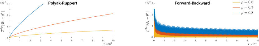
Figure 2: Rates of convergence for PR averaging and Forward-Backward algorithms.

This brings us to the main contributions of this paper:

• It is shown that the “ESC” block in Fig. 1 can be designed to obtain a QSA algorithm for which ${\bar{Y}}=0$, so that the bound $\|\Uptheta_{t}-\theta^{*}\|^{2}=O(t^{-2})$ is obtained.

• The presumption that the rate obtained in (i) is optimal is fallacy. It is shown here that for any $\delta>0$, an algorithm can be designed to achieve $\|\Uptheta_{t}-\theta^{*}\|^{2}=O(t^{-4+\delta})$.

Theory and algorithms are developed for general root finding problems. The theory is refined in the context of gradient free-optimization, and the general theory is illustrated through numerical examples in this setting.

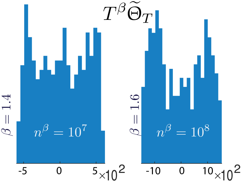
Figure 3: Quasi Monte Carlo using QSA with Polyak-Ruppert averaging. Histograms for $n=10\times T=10^{5}$.

While theory is developed in continuous time, simulation studies using Euler approximations are consistent with theory. The plots shown in Fig. 2 are based on a two-dimensional example, whose details can be found in Section 2.2. The change of notation is also explained there: $(2\rho)^{2}=4-\delta$, where $\rho$ is a design parameter subject to $\rho<1$. In this example ${\bar{Y}}\neq 0$ so that Polyak-Ruppert averaging fails (see (16)). The Forward-backward algorithm is a new algorithm introduced in this paper, that achieves the $O(t^{-4+\delta})$ convergence rate. The plots on the right hand side of Fig. 2 show that $n^{4-\delta}\|\theta_{n}-\theta^{*}\|^{2}$ is bounded in the three experiments shown, where $\theta_{n}$ denotes the Euler approximation at iteration $n$. Standard theory from Quasi-Monte Carlo (QMC) would predict a root mean square convergence rate of $O(\log(n)^{d}/n)$ for QSA in discrete time, since QMC is a special case (see [1, Section 9.3]). It is shown in the present paper that it is possible to obtain $O(n^{-1})$ convergence rate for QMC in discrete time—potentially $O(n^{-\sqrt{4-\delta}})$—subject to a smoothness condition on the function of $\bm{\upxi}$ and careful design of the probing signal. The main results of this paper hinge on these new bounds for QMC.

Fig. 3 illustrates how the techniques introduced in this paper specialize to QMC, based on two instances of the algorithm: one designed using $\beta=\sqrt{4-\delta}=1.4$, and the other with $\beta=1.6$; in the first case it is found empirically that $|\widetilde{\Uptheta}_{T}|\mathbin{:=}|\Uptheta_{T}-\theta^{*}|\leq 10^{3}T^{-1.4}$ for all $T$, provided $|\widetilde{\Uptheta}_{0}|\leq 25$. Details are found in the supplementary material.

Literature Review:  QMC remains an active area of research for applications to estimation and optimization [27]. In standard QMC methodology, a sequence $\{{\scalebox{1.1}{$\upxi$}}_{t}:t\geq 0\}\subset H$ (the $d$-dimensional hypercube $H=[0,1]^{d}$) is constructed so that sample path averages are convergent: $n^{-1}\sum_{1}^{n}f({\scalebox{1.1}{$\upxi$}}_{t})\to\langle f\rangle\mathbin{:=}\int f(x)\,dx$ as $n\to\infty$. The new bounds on the rate of convergence obtained here are based on recent refinements of Baker’s Theorem [22, 10].

QSA was first applied to finance within the context of QMC [18, 19]. Motivated by the successful application of QSA to RL and optimal control in [23], stability theory of general non-linear QSA was first studied in [31] and later advanced in [3, 4]. For one specific choice of gain process $a$, these articles also established convergence rates for the linear case with “additive noise”, of the form $f(\theta,{\scalebox{1.1}{$\upxi$}})=A\theta+B{\scalebox{1.1}{$\upxi$}}$ for matrices $A$ and $B$ of appropriate dimension [31, 4, 3]. The authors in [24, § 4.9] then extended these results significantly, by establishing convergence rates for general non-linear QSA for broader choices of gain processes. Additionally, they introduced acceleration by PR averaging to what was believed to be the optimal MSE rate of $O(T^{-2})$ for this deterministic setting.

Gradient-Free Optimization (GFO) concerns minimization of an objective function $\Upgamma:\mathbb{R}^{d}\to\mathbb{R}$ based solely on measurements of $\Upgamma(\theta)$ for selected values of $\theta\in\mathbb{R}^{d}$. This is motivated by problems in which access to gradient information is computationally intractable or not available (such as in model-free online optimization). The algorithms of Keifer and Wolfowitz are probably the first approaches of this kind [15, 1]. Many improvements followed, with much research led by Spall [32, 33, 34], such as the Simultaneous Perturbation Stochastic Approximation (1SPSA and 2SPSA) algorithms of the form (2) with

$$f^{1\text{SPSA}}(\theta_{n},\zeta_{n}) =\frac{1}{\varepsilon}\zeta_{n+1}\Upgamma(\theta_{n}+\varepsilon\zeta_{n+1})$$ (5)

$$f^{2\text{SPSA}}(\theta_{n},\zeta_{n}) =\frac{1}{2\varepsilon}\bigl{(}\zeta_{n+1}[\Upgamma(\theta_{n}+\varepsilon\zeta_{n+1})-\Upgamma(\theta_{n}-\varepsilon\zeta_{n+1})]\bigr{)}$$

where $\varepsilon>0$ and $\{\zeta_{n}\}$ is a zero-mean i.i.d. sequence. See also [7, 5, 13].

Deterministic versions of SPSA were analyzed in [6] without sharp rates of convergence. The present paper follows the approach of [24, § 4.9], in which the applications to gradient-free optimization result in algorithms that resemble simple versions of the ESC algorithms surveyed in [38, 20].

Notation  Throughout the paper we restrict to sinusoidal probing signals,

$${\scalebox{1.1}{$\upxi$}}_{t}=\sum_{i=1}^{K}v^{i}\cos(2\pi[\ \omega_{i}t+\phi_{i}])$$ (6)

for which $\{\phi_{i}\}$ are arbitrary, and assumptions on the frequencies $\{\omega_{i}\}$ will be imposed in the main results. The vectors $\{v^{i}:1\leq i\leq K\}$ are assumed to span $\mathbb{R}^{m}$.

Let $\Phi_{t}$ denote the function of time evolving on $\mathbb{C}^{K}$ with entries $\Phi_{t}^{i}=\exp(2\pi j[\omega_{i}t+\phi_{i}])$.

For two real-valued functions of time $h,g$ we denote

$$\langle h,g\rangle_{T}\mathbin{:=}\int_{0}^{T}h_{t}g_{t}\,dt\,,\quad\langle h\rangle\mathbin{:=}\lim_{T\to\infty}\frac{1}{T}\int_{0}^{T}h_{t}\,dt\,,\quad\tilde{h}=h-\langle h\rangle\,,\quad h^{\text{\rm\tiny I}}_{T}\mathbin{:=}\int^{T}_{0}\tilde{h}_{t}\,dt-\bar{h}^{\text{\rm\tiny I}}$$ (7)

where $\bar{h}^{\text{\rm\tiny I}}$ is a constant chosen so $\langle h^{\text{\rm\tiny I}}\rangle=0$. When $h$ is a function of time through the probing signal, $h_{t}\equiv h({\scalebox{1.1}{$\upxi$}}_{t})$, then we adopt the alternative notation ${\overline{h}}\mathbin{:=}\langle h({\scalebox{1.1}{$\upxi$}})\rangle$. The bracket notation is also used for vector or matrix valued functions. In particular, we denote $\Sigma_{\text{\tiny${\scalebox{1.1}{$\upxi$}}$}}\mathbin{:=}\langle{\scalebox{1.1}{$\upxi$}}{\scalebox{1.1}{$\upxi$}}^{\intercal}\rangle$, a $K\times K$ matrix. Thm. 2.1 provides conditions ensuring the existence of sample path averages and boundedness of $\{h^{\text{\rm\tiny I}}_{T}:T>0\}$.

For a scalar-valued function $\delta_{t}>0$, we use the notation $O(\delta_{t})$ to denote a vector-valued function of $t$; the notation indicates that there is a constant $B$ such that $\|O(\delta_{t})\|\leq B\delta_{t}$ for all $t$. That is, we are only asserting an upper bound. For example, if $\delta_{t}=1/(1+t)$ we are not claiming that $\|O(\delta_{t})\|\leq B\delta_{t}^{2}$ is not possible.

Organization:  Section 2 surveys recent work and summarizes the main contributions of the paper. Applications to GFO in Section 3 establish new bounds on both bias and convergence rate, along with numerical results illustrating the theory. Conclusions and directions for future research are summarized in Section 4. Technical proofs are postponed to the Appendices.

2 Towards Quartic Rates

2.1 Probing Design for QMC

Thm. 2.1 below justifies boundedness of the integral (7) and much more. Through careful design of the frequencies $\{\omega_{i}\}$ appearing in (6) we can apply refinements of Baker’s Theorem, as surveyed in the monograph [10]. While this theory provides many options, we restrict here to a special case:

$$\omega_{i}=\log(a_{i}/b_{i})>0\,,\ \ 1\leq i\leq K\,,\ \ \textit{where $\{a_{i},b_{i}\}$ are positive integers. }$$ (8)

$$\{\omega_{i}:1\leq i\leq K\}$$ are linearly independent over the field of rational numbers.

Under this assumption $\Sigma_{\text{\tiny${\scalebox{1.1}{$\upxi$}}$}}\mathbin{:=}\langle{\scalebox{1.1}{$\upxi$}}{\scalebox{1.1}{$\upxi$}}^{\intercal}\rangle={\mathchoice{\genfrac{}{}{}{1}{1}{2}}{\genfrac{}{}{}{1}{1}{2}}{\genfrac{}{}{}{3}{1}{2}}{\genfrac{}{}{}{3}{1}{2}}}\sum v^{i}{v^{i}}^{\intercal}$.

Theorem 2.1.

Suppose that the function $h\colon\mathbb{R}^{d}\to\mathbb{R}$ is analytic in a neighborhood of the unit hypercube $[-1,1]^{d}$, and that ${\scalebox{1.1}{$\upxi$}}_{t}$ in (6) satisfies (8). Then the limit defining $\langle h\rangle$ in (7) exists with $h_{t}=h({\scalebox{1.1}{$\upxi$}}_{t})$, and the following ergodic bounds hold for some constant $K_{f}$ independent of the phase values $\{\phi_{i}\}$:

$$\Bigl{|}\frac{1}{T}\int_{0}^{T}\tilde{h}({\scalebox{1.1}{$\upxi$}}_{t})\,dt\Bigr{|} \leq K_{f}\frac{1}{T}\,,\qquad T>0\qquad\textit{where $\tilde{h}=h-\langle h\rangle$. }$$ (9)

Moreover, there is a function ${\hat{h}}\colon\mathbb{C}^{d}\to\mathbb{C}^{d}$ that is analytic in a neighborhood of the domain $\Upomega\mathbin{:=}\{z\in\mathbb{C}^{d}:|z_{i}|=1\,,\ 1\leq i\leq d\}$ satisfying

$$\int_{0}^{T}\tilde{h}({\scalebox{1.1}{$\upxi$}}_{t})\,dt ={\hat{h}}(\Phi_{0})-{\hat{h}}(\Phi_{T})\,,\quad T\geq 0\,,\qquad\bar{h}^{\text{\rm\tiny I}}={\hat{h}}(\Phi_{0})$$ (10)

$$\textit{and}\quad\langle{\hat{h}}(\Phi)\rangle =\lim_{T\to\infty}\frac{1}{T}\int_{0}^{T}{\hat{h}}({\scalebox{1.1}{$\upxi$}}_{t})\,dt=0$$

The function ${\hat{h}}$ is known as a solution to Poisson’s equation with forcing function $\tilde{h}$.

The theorem provides conditions ensuring the existence of $\bar{h}^{\text{\rm\tiny I}}$ and boundedness of $\{h^{\text{\rm\tiny I}}_{T}:T>0\}$ as defined in (7). Since ${\hat{h}}$ is also analytic we are assured of multiple integrals that are also bounded in time. We will require both in the analysis supporting our main results:

$$h^{\text{\rm\tiny I}}_{T}=\int^{T}_{0}\tilde{h}({\scalebox{1.1}{$\upxi$}}_{t})\,dt-\bar{h}^{\text{\rm\tiny I}}=-{\hat{h}}(\Phi_{T})\,,\qquad h^{\text{\rm\tiny II}}_{T}=\int^{T}_{0}h^{\text{\rm\tiny I}}_{t}dt-\bar{h}^{\text{\rm\tiny II}}$$ (11)

The proof of Thm. 2.1 is contained in Appendix B. A few key ideas are presented here: The assumption that $h$ is analytic is imposed so that we can first restrict to complex exponentials, $H(\Phi_{t})=\exp(2\pi jt\omega t)$, whose integral is $H^{\text{\rm\tiny I}}_{t}=(2\pi j\omega)^{-1}H(\Phi_{t})$ when $\omega\neq 0$. In the proof of Thm. 2.1 we use $\omega=\sum_{i=1}^{d}n_{i}\omega_{i}$ with $\{n_{i}\}$ integers; they are not necessarily positive, but at least one $n_{i}$ is assumed non-zero. Extensions of Baker’s Theorem, as surveyed in [10], give a strict lower bound of the form $|\omega|\geq\delta n^{-c}$, where $n=3+\sum|n_{i}|$ and $\delta,c$ are non-negative constants that are independent of $n$—summarized in Thm. B.6. This combined with routine Taylor series bounds establishes the desired conclusions. There is unfortunate news when we search for bounds on $K_{f}$ as a function of dimension. This bound is a function of constants appearing in Thm. B.6, for which present upper bounds grow at least exponentially in $d$. This curse of dimensionality requires application of block descent strategies for applications to optimization in high dimension.

A version of (9) in discrete time is contained in Thm. B.9. This result is a big surprise, given that there is so much theory predicting $O(\log(T)^{d}/T)$ bounds. Much more surprising is that $O(1/T)$ is a very poor rate of convergence for the algorithms developed in this paper, as observed in Fig. 3. Contained in Section 2.4 are examples to show how the theory can be applied to obtain convergence rates of order $O(T^{-2+\delta})$ for specially designed QSA algorithms, and in particular new approaches to QMC.

2.2 Quasi-Stochastic Approximation

Before delving into the main contributions, we summarize the main convergence results for QSA from [24, § 4.9]. For all $\theta\in\mathbb{R}^{d}$, the averaged vector field ${\widebar{f}}$ is defined by the sample path average,

$${\widebar{f}}(\theta) \mathbin{:=}\lim_{T\to\infty}\frac{1}{T}\int^{T}_{0}f(\theta,{\scalebox{1.1}{$\upxi$}}_{t})\,dt$$ (12)

Similar to standard analysis of SA, convergence of the solution of (3) to $\theta^{*}$ is established by comparison with the ODE,

$${\mathchoice{\genfrac{}{}{}{1}{d}{dt}}{\genfrac{}{}{}{1}{d}{dt}}{\genfrac{}{}{}{3}{d}{dt}}{\genfrac{}{}{}{3}{d}{dt}}}\widebar{\Uptheta}_{t}=a_{t}{\widebar{f}}(\widebar{\Uptheta}_{t}),\quad\text{for $t\geq t_{0}$ and $\widebar{\Uptheta}_{t_{0}}=\Uptheta_{t_{0}}$.}$$ (13)

In SA theory the time $t_{0}$ is also a variable, while in QSA theory it is fixed but chosen suitably large for analysis of convergence rates.

The full list of assumptions (QSA1)–(QSA5) may be found in the supplementary material. We settle for a brief summary here: (QSA1) concerns the gain process. In the body of the paper we take $a_{t}=a_{0}(1+t)^{-\rho}$ for $\rho\in(1/2,1]$ and a constant $a_{0}>0$. (QSA2) imposes global Lipschitz bounds on $f$ and ${\widebar{f}}$. (QSA3): the ODE ${\mathchoice{\genfrac{}{}{}{1}{d}{dt}}{\genfrac{}{}{}{1}{d}{dt}}{\genfrac{}{}{}{3}{d}{dt}}{\genfrac{}{}{}{3}{d}{dt}}}\upvartheta_{t}={\widebar{f}}(\upvartheta_{t})$ is globally asymptotically stable. (QSA4): ${\widebar{f}}$ is continuously differentiable, $A(\theta)=\partial_{\theta}{\widebar{f}}\,(\theta)$ is bounded and Lipschitz continuous, and $A^{*}=A(\theta^{*})$ is Hurwitz. (QSA5) includes existence of functions ${\hat{f}}$ and $\widehat{A}$ that are Lipschitz continuous in $\theta$ solving for each $0\leq t_{0}\leq t_{1}$,

$${\hat{f}}(\theta,\Phi_{t_{0}}) =\int_{t_{0}}^{t_{1}}\tilde{f}(\theta,{\scalebox{1.1}{$\upxi$}}_{t})\,dt+{\hat{f}}(\theta,\Phi_{t_{1}})\qquad\widehat{A}(\theta,\Phi_{t_{0}})=\int_{t_{0}}^{t_{1}}\tilde{A}(\theta,{\scalebox{1.1}{$\upxi$}}_{t})\,dt+\widehat{A}(\theta,\Phi_{t_{1}})$$ (14)

where $\tilde{f}(\theta,{\scalebox{1.1}{$\upxi$}}_{t})=f(\theta,{\scalebox{1.1}{$\upxi$}}_{t})-{\widebar{f}}(\theta)$, $\tilde{A}(\theta,{\scalebox{1.1}{$\upxi$}}_{t})=A(\theta,{\scalebox{1.1}{$\upxi$}}_{t})-A(\theta)$ with $A(\theta,{\scalebox{1.1}{$\upxi$}})\mathbin{:=}\partial_{\theta}f\,(\theta,{\scalebox{1.1}{$\upxi$}})$.

A well known approach to acceleration is Polyak-Ruppert (PR) averaging [30, 28, 12, 26, 25]:

$$\Uptheta^{\text{\tiny\sf PR}}_{T}=\frac{1}{T-T_{0}}\int_{T_{0}}^{T}\Uptheta_{t}\,dt$$ (15)

where the interval $[0,T_{0}]$ is known as the burn-in period. This is viewed as a linear time-varying system, and we sometimes opt for the notation $\Uptheta^{\text{\tiny\sf PR}}_{T}=\langle\beta^{\text{\tiny\sf PR}}_{T,\,\cdot\,},\Uptheta\rangle_{T}$, with $\beta^{\text{\tiny\sf PR}}_{T,t}=1/(T-T_{0})$ on $[T_{0},T]$ and zero elsewhere.

General expressions for $\Uptheta_{t}$ and $\Uptheta^{\text{\tiny\sf PR}}_{T}$ obtained in [24, § 4.9] are summarized by the following:

Theorem 2.2.

Suppose that (QSA1)–(QSA5) hold and the following additional assumptions are imposed: $\{\Uptheta_{t}\}$ is obtained using $a_{t}=1/(1+t)^{\rho}$ with $\rho\in(1/2,1)$, and PR averaging is obtained using $T_{0}=(1-1/{\kappa})T$ with $\kappa>1$ fixed. Then there is a vector ${\bar{Y}}\in\mathbb{R}^{d}$ and a bounded zero-mean signal $\{\Xi^{\text{\rm\tiny I}}_{t}\}$ such that

$$\Uptheta_{t} =\theta^{*}+a_{t}[{\bar{Y}}+\Xi^{\text{\rm\tiny I}}_{t}]+o(a_{t})\,,\qquad\Uptheta^{\text{\tiny\sf PR}}_{T}=\theta^{*}+a_{T}c(\kappa,\rho){\bar{Y}}+\mathcal{B}_{T}/T$$ (16)

where $\{\mathcal{B}_{T}\}$ is a bounded process, and

$$c(\kappa,\rho)=\kappa[1-(1-1/\kappa)^{1-\rho}]/(1-\rho)\qquad\Xi^{\text{\rm\tiny I}}_{t}=\int^{t}_{0}f(\theta^{*},{\scalebox{1.1}{$\upxi$}}_{r})\,dr$$

It follows from Thm. 2.2 that $\|\Uptheta_{t}-\theta^{*}\|=O(a_{t})$, and $\|\Uptheta^{\text{\tiny\sf PR}}_{T}-\theta^{*}\|=O(T^{-1})$ if and only if ${\bar{Y}}=0$.

The mysterious vector ${\bar{Y}}$ is defined in terms of another sample path average:

$${\bar{Y}}=[A^{*}]^{-1}\widebar{\Upupsilon},\text{ where}\quad\widebar{\Upupsilon}=-\lim_{T\to\infty}\frac{1}{T}\int^{T}_{0}\bigg{\{}\int^{t}_{0}[A(\theta^{*},{\scalebox{1.1}{$\upxi$}}_{r})-A^{*}]\,dr\bigg{\}}\,f(\theta^{*},{\scalebox{1.1}{$\upxi$}}_{t})\,dt$$ (17)

Existence comes from (14) and (QSA5). Nothing like ${\bar{Y}}$ appears in standard SA theory.

If $A(\theta,{\scalebox{1.1}{$\upxi$}})=A(\theta)$ for all $\theta$ and $\upxi$ then ${\bar{Y}}=0$. This is a very restrictive special case, though it does hold for QMC for which $A(\theta,{\scalebox{1.1}{$\upxi$}})=-I$.

Numerical example:  We demonstrate in the next subsection that the assumptions on the probing signal imposed in Thm. 2.1 are also useful for QSA algorithm design. This would appear far stronger than needed: for one, the full rank condition for $\Sigma_{\text{\tiny${\scalebox{1.1}{$\upxi$}}$}}$ can be achieved under far weaker assumptions. In two dimensions, $\Sigma_{\text{\tiny${\scalebox{1.1}{$\upxi$}}$}}={\mathchoice{\genfrac{}{}{}{1}{1}{2}}{\genfrac{}{}{}{1}{1}{2}}{\genfrac{}{}{}{3}{1}{2}}{\genfrac{}{}{}{3}{1}{2}}}I$ for each of the following special cases: ${\scalebox{1.1}{$\upxi$}}_{t}=[\cos(t),\cos(2t)]^{\intercal}$ and ${\scalebox{1.1}{$\upxi$}}_{t}=[\cos(t),\sin(t)]^{\intercal}$. However, in each case we can construct a second order polynomial $h\colon\mathbb{R}^{2}\to\mathbb{R}$ such that $h({\scalebox{1.1}{$\upxi$}}_{t})=0$ for all $t$, so that the excitation implied by the full rank condition is lost through a simple nonlinearity. This is only the first sign of trouble.

We consider next a numerical example designed with four positive frequencies that are linearly independent over the rationals, denoted $[\omega_{1,1}\,,\,\omega_{2,1}\,,\,\omega_{1,2}\,,\,\omega_{2,2}]$. Consider the linear QSA ODE,

$${\mathchoice{\genfrac{}{}{}{1}{d}{dt}}{\genfrac{}{}{}{1}{d}{dt}}{\genfrac{}{}{}{3}{d}{dt}}{\genfrac{}{}{}{3}{d}{dt}}}\Uptheta_{t}=a_{t}f(\Uptheta_{t},{\scalebox{1.1}{$\upxi$}}_{t})=(1+t)^{-\rho}[(A^{*}+A^{\circ}_{t})\Uptheta_{t}+10b^{\circ}_{t}]$$

$$\textit{with}\quad A^{\circ}_{t}=\begin{bmatrix}4\sin(\omega_{1,1}t)&\sin(\omega_{2,1}t)\\ \sin(\omega_{1,2}t)&4\sin(\omega_{2,2}t)\\ \end{bmatrix}\qquad b^{\circ}_{t}=\begin{bmatrix}2\cos(\omega_{1,1}t)\\ \cos(\omega_{2,2}t)\\ \end{bmatrix}\qquad\textit{and $A^{*}$ Hurwitz. }$$

We have ${\widebar{f}}(\theta)=A^{*}\theta$ and hence $\theta^{*}=0$. To fit the notation above we must take ${\scalebox{1.1}{$\upxi$}}_{t}\in\mathbb{R}^{6}$, which can be chosen so that $\Sigma_{\text{\tiny${\scalebox{1.1}{$\upxi$}}$}}={\mathchoice{\genfrac{}{}{}{1}{1}{2}}{\genfrac{}{}{}{1}{1}{2}}{\genfrac{}{}{}{3}{1}{2}}{\genfrac{}{}{}{3}{1}{2}}}I$. The expression ${\bar{Y}}=-20[2/\omega_{1,1},1/\omega_{2,2}]^{\intercal}$ follows from (17).

The plots shown on the left in Fig. 2 were obtained using PR-averaging applied to this model using $A^{*}=-0.8I$ and frequencies $[\pi\,,\,\sqrt{3}\,,\,4\,,\,\sqrt{5}]/5$. The convergence rate is $O(a_{t})$ because ${\bar{Y}}\neq{\mathchoice{{\mathchoice{\mbox{\large\sf 0}}{\mbox{\large\sf 0}}{\mbox{\tiny\sf 0}}{\mbox{\tiny\sf 0}}}}{\mbox{\sf 0}}{\mbox{\tiny\sf 0}}{\mbox{\tiny\sf 0}}}$.

This bad news is easily avoided by following the guidelines in the next subsection.

2.3 Acceleration

Tighter bounds for PR averaging  Recall from Section 1 that the main contribution of this paper is the introduction of algorithms to achieve MSE bounds that are arbitrarily close to $O(T^{-4})$. The next result asserts that this can be obtained using standard averaging, but only under restrictive conditions.

Proposition 2.3.

Under the assumptions of Thm. 2.2,

$$\Uptheta^{\text{\tiny\sf PR}}_{T}=\theta^{*}+a_{T}[c(\kappa,\rho)+o(1)]{\bar{Y}}+O(T^{-2\rho})$$ (18)

where $c(\kappa,\rho)>0$ is defined below (16). Consequently, $\Uptheta^{\text{\tiny\sf PR}}_{T}$ converges to $\theta^{*}$ with rate $O(T^{-2\rho})$ if and only if ${\bar{Y}}=0$.

Overview of proof: The authors of [11, 24] believed that the best possible convergence rate of $\|\Uptheta^{\text{\tiny\sf PR}}_{T}-\theta^{*}\|$ was $1/T$, and for this simple goal it suffices to establish boundedness of the process $\{\mathcal{B}_{T}\}$ appearing in Thm. 2.2. The proof of (18) begins with the decomposition $\mathcal{B}_{T}=[A^{*}]^{-1}\{\varepsilon^{Y}_{T}-\varepsilon^{Z}_{T}+\varepsilon^{\Upupsilon}_{T}+\varepsilon^{a}_{T}\}$, and then lengthy computations establish that each term is bounded by $O(T^{1-2\rho}+\|{\bar{Y}}\|)$. Thm. 2.2 then completes the proof.     $\sqcap$$\sqcup$

Acceleration by probing design  It is possible to design the probing signal $\bm{\upxi}$ so that ${\bar{Y}}=0$ for general non-linear QSA and hence fast rates can always be achieved:

Theorem 2.4.

If the assumptions of Thm. 2.2 hold and $\bm{\upxi}$ defined in (6) satisfies (8), then ${\bar{Y}}=0$.

Overview of proof: From (17) it suffices to show that $\widebar{\Upupsilon}=0$. For this we combine (14) and (17) to obtain $\widebar{\Upupsilon}_{i}=\bar{z}_{i}$ for each $i$, where $z({\scalebox{1.1}{$\upxi$}})=\widehat{A}(\theta^{*},{\scalebox{1.1}{$\upxi$}})f(\theta^{*},{\scalebox{1.1}{$\upxi$}})\in\mathbb{R}^{d}$ for each ${\scalebox{1.1}{$\upxi$}}\in\mathbb{R}^{m}$. It is shown in Corollary B.5 that steady-state means of this form are always zero under the given assumptions.     $\sqcap$$\sqcup$

Forward-backward filtering  We present a technique to achieve a near quartic MSE convergence rate without imposing additional structure on the probing signal.

Forward-backward (FB) filtering is defined by a pair of QSA ODEs:

$${\mathchoice{\genfrac{}{}{}{1}{d}{dt}}{\genfrac{}{}{}{1}{d}{dt}}{\genfrac{}{}{}{3}{d}{dt}}{\genfrac{}{}{}{3}{d}{dt}}}\Uptheta^{-}_{t} =a_{t}f(\Uptheta^{-}_{t},{\scalebox{1.1}{$\upxi$}}^{-}_{t})\,,\quad\Uptheta^{\text{\tiny\sf PR}^{-}}_{T}=\langle\beta^{\text{\tiny\sf PR}}_{T,\,\cdot\,},\Uptheta^{-}\rangle_{T}$$ (19a)

$$\Uptheta^{\text{\tiny\sf FB}}_{T} ={\mathchoice{\genfrac{}{}{}{1}{1}{2}}{\genfrac{}{}{}{1}{1}{2}}{\genfrac{}{}{}{3}{1}{2}}{\genfrac{}{}{}{3}{1}{2}}}[\Uptheta^{\text{\tiny\sf PR}}_{T}+\Uptheta^{\text{\tiny\sf PR}^{-}}_{T}]$$ (19b)

where ${\scalebox{1.1}{$\upxi$}}^{-}_{t}\mathbin{:=}{\scalebox{1.1}{$\upxi$}}_{-t}$, and $\Uptheta^{\text{\tiny\sf PR}}_{T}$ is defined in (15).

Theorem 2.5.

If the assumptions of Thm. 2.2 hold, then, $\Uptheta^{\text{\tiny\sf FB}}_{T}=\theta^{*}+O(T^{-2\rho})$.

Overview of proof: We refer to ${\scalebox{1.1}{$\upxi$}}_{t}$ as the forward probing signal, and ${\scalebox{1.1}{$\upxi$}}^{-}_{t}$ as backward probing. The analogous vector ${\bar{Y}}$ for the QSA ODE (19a) is denoted ${\bar{Y}}^{-}$. The identity ${\bar{Y}}^{-}=-{\bar{Y}}$ is established through consideration of (17), and the desired bound is then obtained by combining (18) with the definition (19b).     $\sqcap$$\sqcup$

The conclusion of Thm. 2.5 is illustrated in Fig. 2. The plots were obtained using $\kappa=4$ and the three values $\rho\in\{0.6,0.7,0.8\}$. As predicted by Thm. 2.2, PR averaging fails to achieve the convergence rate of $O(T^{-2\rho})$, while FB filtering succeeds for each value of $\rho$ tested.

2.4 Quasi-Monte Carlo

Results from a simple experiment are provided here to illustrate two points: 1/ that Thm. 2.1 can be extended beyond sinusoidal signals, and 2/ in applications to QMC we can design algorithms to achieve convergence rates far faster than $O(\log(n)^{d}/n)$.

Suppose that $\bm{\upxi}$ is $d$-dimensional, with components equal to triangle waves: ${\scalebox{1.1}{$\upxi$}}_{t}^{i}=\bigtriangleup(\omega_{i}t+\phi_{i})$ for each $i$ and $t$, with $\bigtriangleup$ the unit sawtooth wave with unit period and range $\pm 1$:

$$\bigtriangleup(t)=1-4|{\mathchoice{\genfrac{}{}{}{1}{1}{2}}{\genfrac{}{}{}{1}{1}{2}}{\genfrac{}{}{}{3}{1}{2}}{\genfrac{}{}{}{3}{1}{2}}}-\text{frac}\{t+\tfrac{1}{4}\}|$$

Theorem 2.6.

Suppose that $h\colon\mathbb{C}^{d}\to\mathbb{C}$ is analytic in a neighborhood ${\cal N}$ of the hypercube $[-1,1]^{d}$, and suppose that the components of $\bm{\upxi}$ are sawtooth waves with frequencies $\{\omega_{i}\}$ satisfying (8). Then

$$h({\scalebox{1.1}{$\upxi$}}_{t})=h(0)+ \sum_{n=1}^{\infty}\sum_{|\alpha|=n}\frac{1}{\alpha!}h^{(\alpha)}(0){\scalebox{1.1}{$\upxi$}}_{t}^{\alpha}$$

$${\overline{h}}=h(0)+ \sum_{n=1}^{\infty}\sum_{|\alpha|=n}\frac{1}{\alpha!}z^{\alpha}h^{(\alpha)}(0)\widebar{{\scalebox{1.1}{$\upxi$}}^{\alpha}}$$

where

$$\widebar{{\scalebox{1.1}{$\upxi$}}^{\alpha}}=2^{-d}\int_{-1}^{1}\cdots\int_{-1}^{1}t_{1}^{\alpha_{1}}\dots t_{d}^{\alpha_{d}}\,dt_{1}\dots dt_{d}\,,$$

and the following is uniformly bounded in $T>0$:

$$\int_{0}^{T}\tilde{h}({\scalebox{1.1}{$\upxi$}}_{t})\,dt=\sum_{n=1}^{\infty}\sum_{|\alpha|=n}\frac{1}{\alpha!}h^{(\alpha)}(0)\int_{0}^{T}[{\scalebox{1.1}{$\upxi$}}_{t}^{\alpha}-\widebar{{\scalebox{1.1}{$\upxi$}}^{\alpha}}]\,dt$$

The proof is easier than the proof of Thm. 2.1 since we are not searching for conditions for multiple integrals or a solution to Poisson’s equation. The discrete-time counterpart is also straightforward. These results imply the $O(1/T)$ convergence rate for QMC when $h$ is smooth, and it is likely that the QSA theory can also be extended to these probing signals.

We present results from a simple experiment as illustration: Our goal is to estimate the mean of $g(Y)$ with $g\colon\mathbb{R}^{2}\to\mathbb{R}$ and $Y$ uniformly distributed on the rectangle $[-1,1]^{2}$. The probing signal is chosen to be two-dimensional, satisfying the assumptions of Thm. 2.6, so that a QSA algorithm to estimate ${\overline{h}}$ is obtained with $f(\theta,{\scalebox{1.1}{$\upxi$}})=-\theta+h({\scalebox{1.1}{$\upxi$}})$ for which ${\widebar{f}}(\theta)=-\theta+{\overline{h}}$:

$${\mathchoice{\genfrac{}{}{}{1}{d}{dt}}{\genfrac{}{}{}{1}{d}{dt}}{\genfrac{}{}{}{3}{d}{dt}}{\genfrac{}{}{}{3}{d}{dt}}}\Uptheta_{t}=a_{t}[-\Uptheta_{t}+h({\scalebox{1.1}{$\upxi$}}_{t})]$$ (20)

Based on the formula (17) we have ${\bar{Y}}=0$.

Consider the function $h(x_{1},x_{2})=\exp(\gamma x_{1})\sin(2\pi(x_{2}-x_{1}))$, for which ${\overline{h}}=0$ for any value $\gamma$. The frequencies $\{\omega_{1},\omega_{2}\}=\{\log(6),\log(2)\}\approx\{1.8,0.69\}$ were chosen, along with several values of $\rho$, and $\kappa=5$ in application of PR-averaging. The ODEs were approximated using an Euler approximation with sampling time $T_{s}=0.1$ sec., which is roughly 1/5 of the shortest period $1/\omega_{1}$.

The data displayed in LABEL:f:Hist_IID+QSA_p7 is based on four experiments, differentiated by two values $\gamma=1,4$, and choice of probing signal. The first column uses the triangle wave described above, while the second is based on $\{{\scalebox{1.1}{$\upxi$}}_{t_{n}}:n\geq 0\}$ i.i.d. and uniform on $[-1,1]^{2}$, where $\{t_{n}\}$ are the sampling times used in the Euler approximation for QSA. It is known that Polyak-Ruppert averaging shares the same CLT (asymptotic) variance as the usual sample path average when the probing signal is i.i.d.  [28]. The empirical variance using PR averaging was found to be similar to what was obtained using standard Monte Carlo.

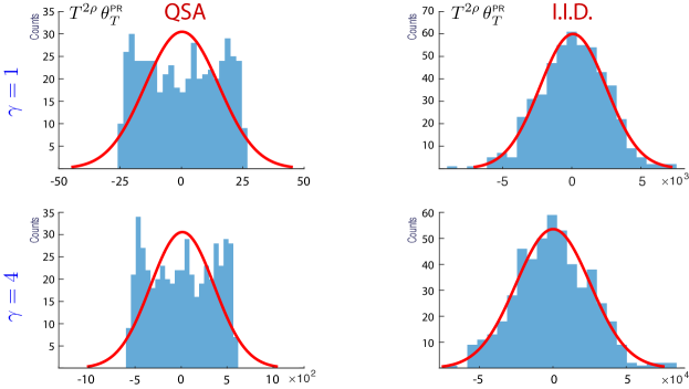
Figure 4: Comparison of Monte Carlo and Quasi-Monte Carlo with Polyak-Ruppert Averaging.

figure]f:Hist_IID+QSA_p7

Each histogram was created based on a runlength of $T=10^{4}$ (corresponding to $10^{5}$ samples, given $T_{s}=0.1$), and 500 independent runs in which the phases were sampled uniformly and independently on $[0,1]$, and the initial condition $\theta_{0}$ was sampled uniformly and independently on $[-25,25]$. The value $\rho=0.7$ was chosen, resulting in $T^{2\rho}\approx 4\times 10^{5}$. The MSE is roughly four orders of magnitude larger for the stochastic algorithm as compared to QSA.

The remaining experiments surveyed here are based on $\gamma=1$.

Fig. 3 shows histograms of the scaled estimation error for Quasi-Monte Carlo with averaging for two cases: $\rho=0.7\,(\beta=1.4)$ and $\rho=0.8\,(\beta=1.6)$. The scaled error exhibits more variability as $\rho$ is increased. In this experiment, the histogram obtained with $\rho=0.8$ is roughly two times wider than for $\rho=0.7$. In other words, the rate of convergence is bounded by a constant $B_{\rho}$ times $T^{-2\rho}$, and in these experiments we observe that the best constant $B_{\rho}$ is an increasing function of $\rho$.

LABEL:f:VerySorry shows sample paths of estimates for standard Monte Carlo and the stochastic PR algorithm, with $\{{\scalebox{1.1}{$\upxi$}}_{t_{n}}:n\geq 0\}$ i.i.d. and uniform.

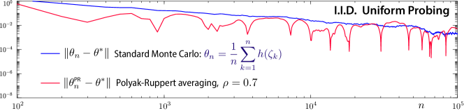
Figure 5: Slow convergence of Monte Carlo and Monte Carlo with Polyak-Ruppert Averaging.

figure]f:VerySorry

The next set of experiments illustrate that the rate of convergence observed in LABEL:f:VerySorry is far slower than observed in any of the deterministic algorithms.

Each row of LABEL:f:notSorry contains four plots: $|\Uptheta_{T}|$ obtained with (20) using the indicated value of $\rho$, $|\Uptheta^{\text{\tiny\sf PR}}_{T}|$ obtained using PR-averaging, and $T^{-\rho}$, $T^{-2\rho}$ as these are the convergence rate bounds for each case. The plots illustrate that the $O(T^{-2\rho})$ bound on the convergence rate using PR averaging is achieved for smaller values of $\rho>1/2$. With $\rho=0.9$ the results are not so clearly compatible with theory; recall that the theory requires $\rho<1$, so we expect numerical challenges when $\rho$ is close to $1$.

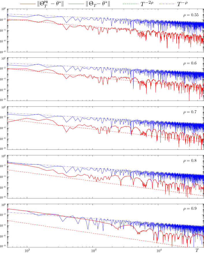
Figure 6: Quasi-Monte Carlo with Polyak-Ruppert Averaging.

figure]f:notSorry

3 Gradient-Free Optimization

3.1 Gradient-Free Optimization and QSA

We now turn to the application of the methods introduced by Section 2 to GFO. It is assumed that the function $\Upgamma$ is $C^{2}$ and that it has a unique minimizer denoted $\theta^{\text{\tiny\sf opt}}$. Two approaches are considered in the following: For $\varepsilon>0$, a $d\times d$ matrix $M>0$ and each $\Uptheta_{0}\in\mathbb{R}^{d}$,

$$\mathbf{1} f^{\text{\rm\tiny$1$Q}}(\Uptheta_{t},{\scalebox{1.1}{$\upxi$}}_{t})=-\frac{1}{\varepsilon}M{\scalebox{1.1}{$\upxi$}}_{t}\Upgamma(\Uptheta_{t}+\varepsilon{\scalebox{1.1}{$\upxi$}}_{t})$$qSGD: (21)

$$\mathbf{2} f^{\text{\rm\tiny$2$Q}}(\Uptheta_{t},{\scalebox{1.1}{$\upxi$}}_{t})=-\frac{1}{2\varepsilon}M{\scalebox{1.1}{$\upxi$}}_{t}[\Upgamma(\Uptheta_{t}+\varepsilon{\scalebox{1.1}{$\upxi$}}_{t})-\Upgamma(\Uptheta_{t}-\varepsilon{\scalebox{1.1}{$\upxi$}}_{t})]$$qSGD: (22)

where $K=m=d$ in (6). These are the natural analogs of Spall’s 1SPSA and 2SPSA algorithms.

The mean vector fields ${\widebar{f}}^{\,\text{1Q}},{\widebar{f}}^{\,\text{2Q}}$ are identical, provided the probing signal is symmetric:

Proposition 3.1.

Suppose (QSA1)-(QSA5) hold and that $\Upgamma$ is $C^{2}$ with unique minimizer $\theta^{\text{\tiny\sf opt}}$. Assume, moreover that $M=\Sigma_{\text{\tiny${\scalebox{1.1}{$\upxi$}}$}}=I$, and that the probing signal is of the form (6) with $\phi_{i}=1/4$ for each $i$. Then, the average vector fields for $1$qSGD and $2$qSGD are equal:

$${\widebar{f}}(\theta)=\langle f^{\text{\rm\tiny$1$Q}}(\theta,{\scalebox{1.1}{$\upxi$}})\rangle=\langle f^{\text{\rm\tiny$2$Q}}(\theta,{\scalebox{1.1}{$\upxi$}})\rangle=-M\Sigma_{\text{\tiny${\scalebox{1.1}{$\upxi$}}$}}\nabla\Upgamma(\theta)+O(\varepsilon^{2})$$ (23)

For notational convenience we set $M=I$ and assume $\Sigma_{\text{\tiny${\scalebox{1.1}{$\upxi$}}$}}=I$ in the subsequent analysis.

For the special case of a strongly convex objective $\Upgamma$, current literature provides bounds on the bias of $2$qSGD [35]. An application of Prop. 3.1 implies that the bias for $1$qSGD is identical:

Corollary 3.2.

Suppose the assumptions of Prop. 3.1 hold, and $\Upgamma$ is strongly convex.
Then, $\|\theta^{*}-\theta^{\text{\tiny\sf opt}}\|\leq O(\varepsilon^{2})$ for either $1$qSGD or $2$qSGD.

3.2 Numerical Examples

We survey results of numerical experiments, whose objective functions were selected from [37]. For a rectangular region $B_{0}\subseteq\mathbb{R}^{d}$, we will frequently use the expression “projection of sample-paths onto $B_{0}$”. This means we project $\Uptheta_{t}$ onto $B_{0}$ component-wise in any approximation of the QSA ODE. For the one-dimensional setting with $B_{0}=[-1,1]$, the projection is defined by $\max\{-1,\min\{1,\theta_{n}\}\}$ where $\theta_{n}$ is an approximation of $\Uptheta_{t_{n}}$ at sampling time $t_{n}$.

Projection is often necessary because Lipschitz continuity of $f$ is assumed in (QSA2). This requires $\Upgamma$ to be Lipschitz continuous when employing $1$qSGD (21) and $\nabla\Upgamma$ when using $2$qSGD (22) [11]. Restricting $\{\Uptheta_{t}\}$ to a closed and bounded set is a way to relax these requirements.

Each experiment contained the following common features:

• The gain process was $a_{t}=\min\{a_{0},(t+1)^{-\rho}\}$ with $1/2\leq\rho\leq 1$, and $a_{0}>0$.

• The QSA parameters $a_{0}$ and $\varepsilon$ were problem specific and chosen by trial and error.

• The ODE (21) was approximated by an Euler scheme with sampling time equal to $1$ sec. This crude approximation is justified via $(\text{i})$ by choosing $a_{0}>0$ sufficiently small.

• Averaging was performed with $\kappa=5$ (prior 20% of samples).

• A rectangular constraint region $B_{0}\subseteq\mathbb{R}^{d}$ was fixed. The selection of $B_{0}$ was based on conventions of the particular objective given in [37].

• For each objective and algorithm, the frequencies were held fixed in $M$ independent experiments: $\{\omega_{i}:1\leq i\leq d\}$ were uniformly sampled from $[0.05,0.5]^{d}$. The initial conditions and phases were not held constant: For $\{1\leq m\leq M\}$,

  • The phases $\{\phi_{i}^{m}:1\leq i\leq d\}$ were sampled uniformly on $[-\pi/2,\pi/2]^{d}$. That is, the probing signal respected $\eqref{e:qSGD_probe}$, and in the $m$th experiment the probing signal took the form

    $${\scalebox{1.1}{$\upxi$}}^{m}_{t}=2[\sin(\omega_{1}t+\phi_{1}^{m})\,,\cdots,\ \sin(\omega_{d}t+\phi_{d}^{m})]^{\intercal}$$

    giving $\Sigma_{\text{\tiny${\scalebox{1.1}{$\upxi$}}$}}=2I$.

  • The initial condition $\Uptheta^{m}_{0}$ were selected uniformly at random from $B_{0}$.

• The outputs were the sample paths $\{\Uptheta^{m}_{t}:t\geq 0\}$, $\{\Upgamma(\Uptheta^{m}_{t}):t\geq 0\}$ and the sample covariance obatined via

  $$\overline{\Sigma}_{T}=\frac{1}{M}\sum_{i=1}^{M}\Uptheta_{T}^{i}{\Uptheta_{T}^{i}}^{\intercal}-\widebar{\Uptheta}_{T}\widebar{\Uptheta}_{T}^{\intercal}\,,\qquad\widebar{\Uptheta}_{T}=\frac{1}{M}\sum_{i=1}^{M}\Uptheta_{T}^{i}$$ (24)

Theory predicts that root mean square error $T^{2\rho}\sqrt{\text{tr}(\overline{\Sigma}_{T})}$ will be bounded in $T$ subject to conditions on the algorithm and probing signal. It is found that the results remain consistent with theory for moderate dimension in each example tested.

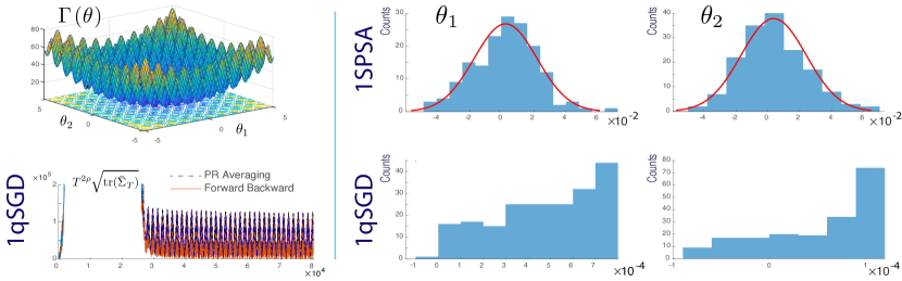
Figure 7: Rastrigin objective (top left), scaled trace of empirical covariance (bottom left), histograms of estimation error for $1$SPSA with PR averaging (top middle and top right), histograms of estimation error for $1$qSGD with PR averaging (bottom middle and bottom right).

Rastrigin:  The experiments illustrated in Figs. 7 and 8 are based on the Rastrigin objective for which $d=2$, and experiments used $T=8\times 10^{4}$, $M=200$ and $a_{0}=0.5$. The projection region was $B_{0}=[-5.12,5.12]^{d}$, following [37]. The two qSGD algorithms were compared in this standard benchmark [37], for which a plot of the objective can be found on the upper left in Fig. 7. In each case the values $\varepsilon=0.25$, $\kappa=5$ and $\rho=0.85$ were used. The stochastic counterparts were included in these experiments in which the exploration sequence $\{\zeta_{n}\}$ was chosen Gaussian and i.i.d., $\mathcal{N}(0,\Sigma)$. The covariance matrix of the stochastic algorithm was chosen so that $\Sigma=\Sigma_{\text{\tiny${\scalebox{1.1}{$\upxi$}}$}}$.

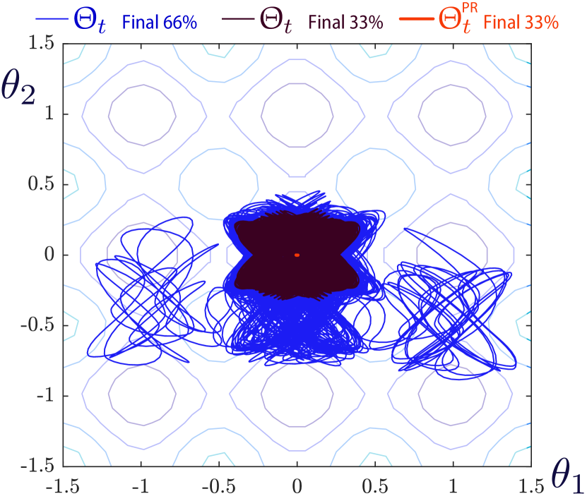
Figure 8: 1qSGD for the Rastrigin objective: $\{\Uptheta_{T}\}$ for the final $66\%$ of the run, and $\{\Uptheta^{\text{\tiny\sf PR}}_{T}\}$ for the final $33\%$.

As predicted by theory, the root-MSE $T^{2\rho}{\rm tr\,}(\widebar{\Sigma}_{T})^{\mathchoice{\genfrac{}{}{}{1}{1}{2}}{\genfrac{}{}{}{1}{1}{2}}{\genfrac{}{}{}{3}{1}{2}}{\genfrac{}{}{}{3}{1}{2}}}$ is bounded in $T$ when using FB filtering or PR averaging: see the plot on the lower left in Fig. 7. Apart from achieving near quartic convergence rates, the estimates of $\theta^{\text{\tiny\sf opt}}$ resulting from the deterministic algorithm had less variability than their stochastic counterpart. This reduction of variability was roughly two orders of magnitude. In both cases, the histograms show that the algorithms consistently overestimate $\theta^{\text{\tiny\sf opt}}$. This is most likely due to the bias that is inherent in these algorithms (recall Section 3.1).

Histograms are shown only for $1$qSGD and $1$SPSA using PR-averaging. The results obtained for $1$qSGD with FB filtering were similar. Results obtained using $2$qSGD and $2$SPSA were similar qualitatively. Outliers were identified with Matlab’s isoutlier function and excluded in these plots. Outliers were found in 20% of the independent runs for $1$SPSA, and none for $1$qSGD. Outliers for deterministic algorithms were observed in other experiments, but fewer than in their stochastic counterparts.

Fig. 8 shows part of the trajectory of $\{\Uptheta_{T}\}$ for a short run for better vizualization. We see that $\{\Uptheta_{T}\}$ oscillates between saddle points and local extrema before settling around the minimizer $\theta^{\text{\tiny\sf opt}}=0$ near the end of the run. The corresponding PR-estimates very closely approximate $\theta^{\text{\tiny\sf opt}}$ for the final 33% of the run.

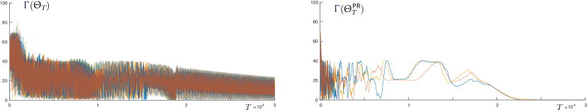
Figure 9: Evolution of $\Upgamma(\Uptheta_{T})$ (left) and $\Upgamma(\Uptheta^{\text{\tiny\sf PR}}_{T})$ (right) as functions of $T$ for the Rastrigin objective.

figure]fig:Rasta_Loss

The plots in LABEL:fig:Rasta_Loss show a comparison of both $\Upgamma(\Uptheta_{T})$ and $\Upgamma(\Uptheta^{\text{\tiny\sf PR}}_{T})$ for three distinct initial conditions $\Uptheta_{0}$. This plot illustrates the benefits of PR averaging as $\Upgamma(\Uptheta^{\text{\tiny\sf PR}}_{T})$ approaches $\Upgamma(\theta^{*})=0$ much quicker than $\Upgamma(\Uptheta_{T})$ for each initial condition.

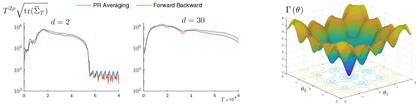
Figure 10: Scaled root-MSE for $d=2$ (left) and $d=30$ (middle). At right is the Ackley objective for $d=2$.

figure]f:Ackley

Ackley:  This is another standard benchmark [37], whose objective function is shown on the right in LABEL:f:Ackley in the special case $d=2$. We performed $M=50$ independent experiments of run length $T=8\times 10^{4}$ to minimize the Ackley objective with projection region equal to $B_{0}=[-32.768,32.768]^{d}$ [37]. Experiments only employed $1$qSGD and were performed for two sets of parameters:

• $\rho=0.85$, $a_{0}=0.02$ and $\varepsilon=0.01$.

• $\rho=0.7$, $a_{0}=0.07$ and $\varepsilon=0.1$.

For each set of parameters, the root mean square error $T^{2\rho}\sqrt{\text{tr}(\overline{\Sigma}_{T})}$ was obtained for $d=2$ and $d=30$. Results for case (i) are pictured in LABEL:f:Ackley and repeated in LABEL:f:Ackley_08507_cov along with results for case (ii). Both PR averaging and FB filtering are successful in achieving $O(T^{-2\rho})$ convergence rates.

However, we see that in case (i) ${\rm tr\,}(\widebar{\Sigma}_{T})^{\mathchoice{\genfrac{}{}{}{1}{1}{2}}{\genfrac{}{}{}{1}{1}{2}}{\genfrac{}{}{}{3}{1}{2}}{\genfrac{}{}{}{3}{1}{2}}}$ appears to approach a steady-state only for $d=2$, suggesting that the run length is not sufficiently large for $d=30$ with $\rho=0.85$. For case (ii), the empirical covariances appear to approach a steady-state value for both $d=2$ and $d=30$. As expected by the discussion on the curse of dimension for QSA after Thm. 2.1, the steady-state value of ${\rm tr\,}(\widebar{\Sigma}_{T})^{\mathchoice{\genfrac{}{}{}{1}{1}{2}}{\genfrac{}{}{}{1}{1}{2}}{\genfrac{}{}{}{3}{1}{2}}{\genfrac{}{}{}{3}{1}{2}}}$ grows with $d$.

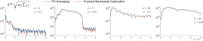
Figure 11: Comparison of scaled empirical covariances for Ackley objective.

figure]f:Ackley_08507_cov

Figure 12: Average of $\Upgamma(\Uptheta^{i}_{T})$ over $1\leq i\leq M$ independent runs for the three-hump camel objective.

figure]f:3humpObj

Three-Hump Camel:  This standard $d=2$ dimensional benchmark, plotted on the right in LABEL:f:3humpObj, uses $B_{0}=[-5,5]^{d}$ [37].

Results from the $1$qSGD algorithm are surveyed here, for the values $\rho=0.85$ and $\rho=0.7$; in each of these two cases the values $a_{0}=0.01$ and $\varepsilon=0.5$ were successful. Covariance estimates were obtained based on $M=50$ independent experiments with run length $T=8\times 10^{4}$.

The average loss plotted in LABEL:f:3humpObj was obtained via

$$\bar{\Upgamma}_{T}=\frac{1}{M}\sum^{M}_{m=1}\Upgamma(\Uptheta^{m}_{T})$$

with estimates $\{\Uptheta^{m}_{t}:t\geq 0\}$ obtained using PR-averaging. We find that the value $\Upgamma(\Uptheta^{\text{\tiny\sf PR}}_{t})$ converges rapidly towards its optimal value of zero. The results for this experiment agree with the previous observations: near quartic rates are achieved. The steady-state value of ${\rm tr\,}(\widebar{\Sigma}_{T})^{\mathchoice{\genfrac{}{}{}{1}{1}{2}}{\genfrac{}{}{}{1}{1}{2}}{\genfrac{}{}{}{3}{1}{2}}{\genfrac{}{}{}{3}{1}{2}}}$ appears to grow with $\rho$.

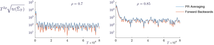
Figure 13: Scaled empirical covariances for $\rho=0.7$ (left) and $\rho=0.85$ (right) for three-hump camel objective.

figure]f:3Hump_2dim08507cov

4 Conclusions

While it is convenient to design exploration around i.i.d. signals, and this approach opens the doors to many powerful tools from probability theory, we have shown that deterministic “noise” has significant benefits. Convergence rates can be accelerated dramatically provided the algorithm and deterministic probing signals are chosen with care.

There are many avenues for future research:

$\triangle$  QSA algorithms appear to suffer from the curse of dimensionality that is well known in QMC [1]. We have found in experiments that the run length $T>0$ must be very large to see the benefit of the $O(T^{-2\rho})$ bound when $d$ is large, or $\rho>0.9$. Future refinements of these algorithms will be motivated by these shortcomings.

$\triangle$  The optimal convergence rate for QSA is still unknown. The rates obtained in this paper are only upper bounds. It is possible that the optimal convergence rate for QSA algorithms is actually faster than $O(T^{-2\rho})$; in fact, the rate $O(T^{-1-\rho})$ is conjectured based on recent analysis.

$\triangle$  It is not clear that the constraint $\rho>{\mathchoice{\genfrac{}{}{}{1}{1}{2}}{\genfrac{}{}{}{1}{1}{2}}{\genfrac{}{}{}{3}{1}{2}}{\genfrac{}{}{}{3}{1}{2}}}$ is required in this deterministic setting, and may be removed if we can improve the bounds in our analysis. We have found in some experiments that the use of PR averaging results in very fast convergence even when this constraint is violated.

$\triangle$  In stochastic optimization it is common to choose $\rho=0$ (a constant gain or step-size). Stability theory and convergence rate bounds with averaging is another topic of research. We conjecture that bounds may be simple when noise is purely additive, following [25, 26].

$\triangle$  Under what conditions is $\sqrt{\text{tr}(\overline{\Sigma}_{T})}$ strictly smaller using the FB algorithm as compared to PR averaging? We find in experiments that the FB algorithm usually outperforms the others, but we have yet to find tools to provide bounds that are rich enough to compare algorithms.

Appendix A Assumptions for QSA Theory

The assumptions imposed in [24, § 4.9] are listed below. The setting there is far more general than here, since the entries of the probing signal are not restricted to mixtures of sinusoids. In this prior work it is assumed that the probing signal is a function of a deterministic signal $\Phi$ of the form ${\scalebox{1.1}{$\upxi$}}_{t}=G(\Phi_{t})$, where $\Phi$ is the state process for a dynamical system,

$${\mathchoice{\genfrac{}{}{}{1}{d}{dt}}{\genfrac{}{}{}{1}{d}{dt}}{\genfrac{}{}{}{3}{d}{dt}}{\genfrac{}{}{}{3}{d}{dt}}}\Phi_{t}=\text{H}(\Phi_{t})$$ (25)

with $\text{H}\colon\Upomega\to\Upomega$ and $\Upomega$ is a compact subset of the Euclidean space. It is assumed that it has a unique invariant measure $\uppi$ on $\Upomega$.

For the special case treated here, with $\Phi_{t}^{i}=\exp(2\pi j[\omega_{i}t+\phi_{i}])$ for each $i$ and $t$, we have $\Upomega=S^{K}\subset\mathbb{C}$ with $S$ the unit circle in $\mathbb{C}$. The dynamics (25) and the function $G$ are linear:

$${\mathchoice{\genfrac{}{}{}{1}{d}{dt}}{\genfrac{}{}{}{1}{d}{dt}}{\genfrac{}{}{}{3}{d}{dt}}{\genfrac{}{}{}{3}{d}{dt}}}\Phi_{t} =W\Phi_{t}\qquad W\mathbin{:=}2\pi j\text{\rm diag}(\omega_{i})$$ (26)

$${\scalebox{1.1}{$\upxi$}}_{t} =G(\Phi_{t})\qquad G(z)\mathbin{:=}{\mathchoice{\genfrac{}{}{}{1}{1}{2}}{\genfrac{}{}{}{1}{1}{2}}{\genfrac{}{}{}{3}{1}{2}}{\genfrac{}{}{}{3}{1}{2}}}V(z+z^{-1})\,,\qquad z\in\mathbb{C}^{d}$$

where $V$ is the $d\times d$ matrix whose $i$th column is equal to the vector $v^{i}$ appearing in (6).

The following is assumed to streamline notation throughout the remainder of this document:

$$K=m=d$$   in the definition (6).

Recall that this is required for the algorithms introduced in Section 3.1.

The proof of Prop. B.1 below begins with a proof that $\uppi$ exists, with density $\uprho(z_{1},\dots,z_{d})=\prod_{i=1}^{d}u(z_{i})$, where $u$ denotes the uniform distribution on $S$. In particular, since ${\scalebox{1.1}{$\upxi$}}_{t}=G(\Phi_{t})$ for some function $G$, the function ${\widebar{f}}$ in (12) can be expressed,

$${\widebar{f}}(\theta)=\int_{\Upomega}f(\theta,G(z))\,\uppi(dz)$$ (27)

The remaining assumptions are listed below. The bound in (28b) and those in (QSA5) are partially justified by Thm. 2.1 subject to smoothness assumptions on $f$.

(QSA1)  The process $a$ is non-negative, monotonically decreasing, and

$$\lim_{t\to\infty}a_{t}=0,\qquad\int_{0}^{\infty}a_{r}\,dr=\infty.$$ (28a)

(QSA2)  The functions ${\widebar{f}}$ and $f$ are Lipschitz continuous: for a constant $L_{f}<\infty$,

$$\|{\widebar{f}}(\theta^{\prime})-{\widebar{f}}(\theta)\| \leq L_{f}\|\theta^{\prime}-\theta\|,$$

$$\|f(\theta^{\prime},{\scalebox{1.1}{$\upxi$}})-f(\theta,{\scalebox{1.1}{$\upxi$}})\| \leq L_{f}\|\theta^{\prime}-\theta\|,\quad\theta^{\prime},\,\theta\in\mathbb{R}^{d}\,,{\scalebox{1.1}{$\upxi$}}\in\mathbb{R}^{m}$$

There exists a Lipschitz continuous function $b_{0}\colon\mathbb{R}^{d}\to\mathbb{R}_{+}$, such that for all $\theta\in\mathbb{R}^{d}$,

$$\bigg{\|}\int_{t_{0}}^{t_{1}}\tilde{f}_{t}(\theta)\,dt\bigg{\|}\leq b_{0}(\theta)\,,\quad 0\leq t_{0}\leq t_{1}\,,\qquad\textit{where}\quad\tilde{f}_{t}(\theta)=f(\theta,{\scalebox{1.1}{$\upxi$}}_{t})-{\widebar{f}}(\theta)$$ (28b)

(QSA3)  The ODE ${\mathchoice{\genfrac{}{}{}{1}{d}{dt}}{\genfrac{}{}{}{1}{d}{dt}}{\genfrac{}{}{}{3}{d}{dt}}{\genfrac{}{}{}{3}{d}{dt}}}\upvartheta_{t}={\widebar{f}}(\upvartheta_{t})$ is globally asymptotically stable with unique equilibrium $\theta^{*}$.

(QSA4)  The vector field ${\widebar{f}}$ is differentiable, with derivative denoted

$$A(\theta)=\partial_{\theta}{\widebar{f}}\,(\theta)$$ (28c)

That is, $A(\theta)$ is a $d\times d$ matrix for each $\theta\in\mathbb{R}^{d}$, with $\displaystyle A_{i,j}(\theta)=\frac{\partial}{\partial\theta_{j}}{\widebar{f}}_{i}\,(\theta)$.

Moreover, the derivative $A$ is Lipschitz continuous, and $A^{*}=A(\theta^{*})$ is Hurwitz.

(QSA5)  $\Phi$ satisfies the following ergodic theorems for the functions of interest, for each initial condition $\Phi_{0}\in\Upomega$:

• For each $\theta$ there exists a solution ${\hat{f}}(\theta,\,\cdot\,)$ to Poisson’s equation with forcing function $\tilde{f}(\theta,\,\cdot\,)=f(\theta,\,\cdot\,)-{\widebar{f}}(\theta)$. That is,

  $${\hat{f}}(\theta,\Phi_{t_{0}})=\int_{t_{0}}^{t_{1}}\tilde{f}(\theta,{\scalebox{1.1}{$\upxi$}}_{t})\,dt+{\hat{f}}(\theta,\Phi_{t_{1}})\,,\qquad 0\leq t_{0}\leq t_{1}$$ (28d)

  with ${\widebar{f}}$ given in (27) and $\int_{\Upomega}{\hat{f}}(\theta,z)\,\,\uppi(dz)={\mathchoice{{\mathchoice{\mbox{\large\sf 0}}{\mbox{\large\sf 0}}{\mbox{\tiny\sf 0}}{\mbox{\tiny\sf 0}}}}{\mbox{\sf 0}}{\mbox{\tiny\sf 0}}{\mbox{\tiny\sf 0}}}$.

• The function ${\hat{f}}$, and derivatives $\partial_{\theta}{\widebar{f}}$ and $\partial_{\theta}f$ are Lipschitz continuous in $\theta$. In particular, ${\hat{f}}$ admits a derivative $\widehat{A}$, which is assumed to be $C^{1}$ and to satisfy

  $$\widehat{A}(\theta,\Phi_{t_{0}})=\int_{t_{0}}^{t_{1}}[A(\theta,{\scalebox{1.1}{$\upxi$}}_{t})-A(\theta)]\,dt+\widehat{A}(\theta,\Phi_{t_{1}})\,,\qquad 0\leq t_{0}\leq t_{1}$$ (28e)

  where $A(\theta,{\scalebox{1.1}{$\upxi$}})=\partial_{\theta}f(\theta,{\scalebox{1.1}{$\upxi$}})$, and $A(\theta)=\partial_{\theta}{\widebar{f}}\,(\theta)$ was defined in (28c). Lipschitz continuity is assumed uniform with respect to the probing signal: for $L_{f}<\infty$,

  $$\|{\hat{f}}(\theta^{\prime},\Phi)-{\hat{f}}(\theta,\Phi)\| \leq L_{f}\|\theta^{\prime}-\theta\|$$

  $$\|A(\theta^{\prime},{\scalebox{1.1}{$\upxi$}})-A(\theta,{\scalebox{1.1}{$\upxi$}})\| \leq L_{f}\|\theta^{\prime}-\theta\|$$

  $$\|\widehat{A}(\theta^{\prime},\Phi)-\widehat{A}(\theta,\Phi)\| \leq L_{f}\|\theta^{\prime}-\theta\|,\qquad\theta^{\prime},\,\theta\in\mathbb{R}^{d}\,\,,{\scalebox{1.1}{$\upxi$}}\in\mathbb{R}^{m},\ \Phi\in\Upomega$$

• $$\Xi^{\text{\rm\tiny I}}_{T}(\theta) \mathbin{:=}\int_{0}^{T}[f(\theta,{\scalebox{1.1}{$\upxi$}}_{t})-{\widebar{f}}(\theta)]\,dt={\hat{f}}(\theta,\Phi_{0})-{\hat{f}}(\theta,\Phi_{T})$$ (28f)

  $$\Upupsilon(\theta,\Phi_{t}) \mathbin{:=}[\widehat{A}(\theta,\Phi_{0})-\widehat{A}(\theta,\Phi_{t})]f(\theta,{\scalebox{1.1}{$\upxi$}}_{t})=\partial_{\theta}\Xi^{\text{\rm\tiny I}}_{t}\,(\theta)\cdot f(\theta,{\scalebox{1.1}{$\upxi$}}_{t})$$ (28g)

  with $\Xi^{\text{\rm\tiny I}}_{T}(\theta^{*})=\Xi^{\text{\rm\tiny I}}_{T}$ and $\Upupsilon(\theta^{*},\Phi_{t})=\Upupsilon_{t}$.

  The following limit exists:

  $$\widebar{\Upupsilon}\mathbin{:=}\langle\Upupsilon(\theta^{*},\Phi)\rangle=-\int_{\Upomega}\widehat{A}(\theta^{*},z)f(\theta^{*},G(z))\,\uppi(dz)$$ (28h)

  and the following integrals are bounded in $t$:

  $${\Upupsilon}^{\text{\rm\tiny I}}_{t}=\int_{0}^{t}[\Upupsilon_{r}-\widebar{\Upupsilon}]\,dr-\widebar{{\Upupsilon}^{\text{\rm\tiny I}}}_{t}\,,\qquad\Xi^{\text{\rm\tiny II}}_{t}=\int_{0}^{t}\Xi^{\text{\rm\tiny I}}_{r}\,dr-\widebar{\Xi^{\text{\rm\tiny II}}}_{t}$$ (28i)

Appendix B Technical Proofs

B.1 Tighter Bounds for Quasi-Monte Carlo

We begin with a characterization of ${\overline{h}}=\langle h\rangle$ with $h_{t}=h({\scalebox{1.1}{$\upxi$}}_{t})$, using the probing signal (6).

An Elementary Ergodic Theorem  The ergodic theorems presented here is based upon a stationary relaxation of the solution to the ODE ${\mathchoice{\genfrac{}{}{}{1}{d}{dt}}{\genfrac{}{}{}{1}{d}{dt}}{\genfrac{}{}{}{3}{d}{dt}}{\genfrac{}{}{}{3}{d}{dt}}}\Phi_{t}=W\Phi_{t}$ (recall (26)).

Suppose that the initial conditions $\{\Phi_{0}^{i}:1\leq i\leq d\}$ are chosen randomly with i.i.d. values uniform on the unit circle $S\subset\mathbb{C}$. It follows that $\{\Phi_{t}^{i}:1\leq i\leq d\}$ remain i.i.d.  with uniform distribution for each $t\in\mathbb{R}$, so that ${\mathchoice{\mbox{\boldmath$\Phi$}}{\mbox{\boldmath$\Phi$}}{\mbox{\boldmath$\scriptstyle\Phi$}}{\mbox{\boldmath$\scriptscriptstyle\Phi$}}}=\{\Phi_{t}:-\infty<t<\infty\}$ is a stationary Markov process. Stationarity implies the Law of Large Numbers: for any Borel measurable function $H\colon S^{d}\to\mathbb{C}$,

$$\lim_{T\to\infty}\frac{1}{T}\int_{0}^{T}H(\Phi_{t})\,dt=\lim_{T\to\infty}\frac{1}{T}\int_{0}^{T}H(\Phi_{-t})\,dt=\textrm{E}[H(\Phi_{0})]=\int_{S^{d}}H(z)\,dz\qquad a.s.$$ (29)

Conditioning on $\Phi_{0}=z^{0}$ we can extend this limit to a.e. initial condition $z^{0}\in S^{d}$.

Consider any real-valued function $h$ of the probing signal (6). We have $h({\scalebox{1.1}{$\upxi$}}_{t})=H(\Phi_{t})$ with $H\mathbin{:=}h\circ G$ from (26), which then implies a law of large numbers. An alternative characterization of the limit is found in terms of the $d\times d$ matrix $V$ defined below (26), and a $d$-dimensional random vector denoted $X$ whose entries are i.i.d. with the arcsine law on $[-\pi,\pi]$.

Proposition B.1.

Consider any Borel measurable function $h\colon\mathbb{R}^{d}\to\mathbb{R}$ satisfying ${\sf E}[|h(VX)|]<\infty$. The following limits then hold for a.e. set of phase angles $\{\phi_{i}\}$:

$$\lim_{T\to\infty}\frac{1}{T}\int_{0}^{T}h({\scalebox{1.1}{$\upxi$}}_{t})\,dt=\lim_{T\to\infty}\frac{1}{T}\int_{0}^{T}h({\scalebox{1.1}{$\upxi$}}_{-t})\,dt={\sf E}[h(VX)]$$ (30)

If in addition the function $h$ is continuous, then (30) holds for each initial condition, and convergence is uniform in the initial phase angles.

Proof.

The result (30) for a.e. initial condition $\Phi_{0}$ is immediate from (29).

If $h$ is continuous then we make explicit the dependency of the average on the initial condition as follows:

$$h_{t}(\Phi_{0})\mathbin{:=}h(G(e^{Wt}\Phi_{0}))=h({\scalebox{1.1}{$\upxi$}}_{t})\,,\qquad{\overline{h}}_{T}(\Phi_{0})\mathbin{:=}\frac{1}{T}\int_{0}^{T}h_{t}(\Phi_{0})\,dt$$

We show that $\{h_{t}:t>0\}$ and $\{{\overline{h}}_{t}:t>0\}$ are each equicontinuous families of functions on $\Upomega$. Since $e^{Wt}$ is an isometry on $\mathbb{C}^{d}$ for any $t$, there exists a $K_{v}<\infty$ such that:

$$\|G(e^{Wt}z)-G(e^{Wt}z^{\prime})\|<K_{v}\|z-z^{\prime}\|,\quad\text{for $z,z^{\prime}\in\mathbb{C}^{d}$ and $t>0$}$$ (31)

Now, $h$ is uniformly continuous on $\Upomega$ since this domain is compact: for each $\varepsilon>0$, there exists $\delta>0$ such that:

$$\|h(z)-h(z^{\prime})\|<\delta,\quad\text{if }\|z-z^{\prime}\|<\varepsilon$$

Thus, by (31),

$$\|h(z)-h(z^{\prime})\|<\delta,\quad\text{if }\|z-z^{\prime}\|<\varepsilon/K_{v}$$

Equicontinuity of $\{h_{t}:t>0\}$ and $\{{\overline{h}}_{t}:t>0\}$ on $\Upomega$ follows from these bounds. ${\overline{h}}_{T}$ converges pointwise to $\langle h\rangle$ for a.e. $\Phi_{0}\in\Upomega$ as $T\to\infty$. The combination of these results implies convergence from each initial condition, and also uniform convergence:

$$\lim_{T\to\infty}\max_{\Phi_{0}\in\Upomega}\|{\overline{h}}_{T}(\Phi_{0})-\langle h\rangle\|=0$$

$\sqcap$$\sqcup$

This proposition will be refined in the following.

If $h\colon\mathbb{R}^{d}\to\mathbb{R}$ is analytic in a neighborhood of $z\in\mathbb{R}^{d}$, we denote the mixed partials by

$$h^{(\alpha)}(z)=\frac{\partial^{\alpha_{1}}}{\partial z_{1}^{\alpha_{1}}}\cdots\frac{\partial^{\alpha_{d}}}{\partial z_{d}^{\alpha_{d}}}h\,(z)\,,\quad\alpha\in\mathbb{Z}_{+}^{d}\,.$$

Denote $z^{\alpha}=\prod_{i}z_{i}^{\alpha_{i}}$, and $\alpha!=\prod_{i}\alpha_{i}!$ for $\alpha\in\mathbb{Z}_{+}^{d}$ with $0!\mathbin{:=}1$. This notation is used to express the multivariate Taylor series formula in the following:

Lemma B.2.

Suppose that $h\colon\mathbb{C}^{d}\to\mathbb{R}$ is analytic in a neighborhood ${\cal N}$ of the hypercube $[-1,1]^{d}$. Then there is $r_{h}>1$ such that whenever $z\in[-1,1]^{d}$ and $0\leq r\leq r_{h}$ we have

$$h(rz)=h(0)+ \sum_{n=1}^{\infty}r^{n}\sum_{|\alpha|=n}\frac{1}{\alpha!}z^{\alpha}h^{(\alpha)}(0)$$ (32a)

where the sum converges absolutely: $$\sum_{n=1}^{\infty}r_{h}^{n}\sum_{|\alpha|=n}\frac{1}{\alpha!}|h^{(\alpha)}(0)|<\infty$$ (32b)

Lemma B.2 provides a representation of both $h({\scalebox{1.1}{$\upxi$}}_{t})$ and the integral $\tilde{h}({\scalebox{1.1}{$\upxi$}}_{t})=h({\scalebox{1.1}{$\upxi$}}_{t})-{\overline{h}}$. A useful representation requires more notation.

To further streamline notation we assume that $v^{i}=e^{i}$ for each $i$, so that $V$ is the identity matrix; this is without any loss of generality since we can replace $h(z)$ by $\check{h}(z)=h(V^{-1}z)$ under the standing assumption that $V$ is full rank. Under this convention it follows that

$$h({\scalebox{1.1}{$\upxi$}}_{t})=h({\scalebox{1.1}{$\upxi$}}_{t}^{1},\dots,{\scalebox{1.1}{$\upxi$}}_{t}^{d}\bigr{)}\,,\quad t\geq 0\,,\qquad\textit{ with \ \ ${\scalebox{1.1}{$\upxi$}}_{t}^{i}=\cos(2\pi[\omega_{i}t+\phi_{i}])$ \ \ for $1\leq i\leq d$. }$$

For $\alpha\in\mathbb{Z}_{+}^{d}$ we denote

$${\scalebox{1.1}{$\upxi$}}_{t}^{\alpha} =\prod_{i=1}^{d}\cos(2\pi[\omega_{i}t+\phi_{i}])^{\alpha_{i}}=2^{-|\alpha|}\prod_{i=1}^{d}({\scalebox{1.1}{$\upxi$}}_{t}^{i}+{{\scalebox{1.1}{$\upxi$}}_{t}^{i}}^{*})^{\alpha_{i}}$$ (33)

$$=\langle{\scalebox{1.1}{$\upxi$}}^{\alpha}\rangle\,,\qquad\widetilde{{\scalebox{1.1}{$\upxi$}}}_{t}^{\alpha}={\scalebox{1.1}{$\upxi$}}_{t}^{\alpha}-\widebar{{\scalebox{1.1}{$\upxi$}}^{\alpha}}$$

where $|\alpha|=\sum\alpha_{i}$ (the $\ell_{1}$-norm), and ${{\scalebox{1.1}{$\upxi$}}_{t}^{i}}^{*}$ denotes the complex conjugate. Let $B$ denote the set of all $d$-dimensional row vectors with entries in $\{-1,1\}$. For fixed $\alpha\in\mathbb{Z}_{+}^{d}$, $|\alpha|\neq 0$, we decompose $b\in B$ as follows: $b=(b^{1},b^{2},\dots,b^{d})$, where $b^{i}$ has length $\alpha_{i}$ for each $i$, and necessarily has entries in $\{-1,1\}$. These are used to define the frequency and phase variables

$$\omega_{\alpha,b}=\sum_{i=1}^{d}\alpha_{i}\omega_{i}\sum_{k}b^{i}_{k}\qquad\phi_{\alpha,b}=\sum_{i=1}^{d}\alpha_{i}\phi_{i}\sum_{k}b^{i}_{k}$$ (34)

Let $B_{0}^{\alpha}\subset B$ denote the set of vectors $b\in B$ for which $\omega_{\alpha,b}=0$. Under the assumption that the frequencies are linearly independent over the rationals, this is equivalent to the following requirement:

$$\alpha_{i}\sum_{k}b^{i}_{k}=0\,\quad\textit{for each $1\leq i\leq d$}$$

Lemma B.3.

The signal $\{{\scalebox{1.1}{$\upxi$}}^{\alpha}_{t}\}$, its mean, and its centered integral admit the representations,

$${\scalebox{1.1}{$\upxi$}}^{\alpha}_{t} =2^{-|\alpha|}\sum_{b\in B^{\alpha}}{\scalebox{1.1}{$\upxi$}}_{t}^{\alpha,b}\,,\qquad\qquad\widebar{{\scalebox{1.1}{$\upxi$}}^{\alpha}}=2^{-|\alpha|}\sum_{b\in B_{0}^{\alpha}}\exp(j\phi_{\alpha,b})$$ (35)

$${\scalebox{1.1}{$\upxi$}}^{\alpha\text{\rm\tiny I}}_{t} =2^{-|\alpha|}\sum_{b\not\in B_{0}^{\alpha}}\frac{1}{2\pi j\omega_{\alpha,b}}{\scalebox{1.1}{$\upxi$}}_{t}^{\alpha,b}\,,\qquad{\scalebox{1.1}{$\upxi$}}_{t}^{\alpha,b}=\exp(2\pi j[\omega_{\alpha,b}t+\phi_{\alpha,b}])$$

Proof.

The representation for ${\scalebox{1.1}{$\upxi$}}^{\alpha}_{t}$ is purely a change of notation. We have ${\scalebox{1.1}{$\upxi$}}_{t}^{\alpha,b}=\exp(j\phi_{\alpha,b})$ (independent of $t$) when $b\in B_{0}$, and $\langle{\scalebox{1.1}{$\upxi$}}^{\alpha,b}\rangle=0$ otherwise. Consequently,

$$=2^{-|\alpha|}\sum_{b\in B^{\alpha}}\langle{\scalebox{1.1}{$\upxi$}}^{\alpha,b}\rangle=2^{-|\alpha|}\sum_{b\in B_{0}^{\alpha}}\exp(j\phi_{\alpha,b})$$

$${\scalebox{1.1}{$\upxi$}}^{\alpha\text{\rm\tiny I}}_{t} =\int^{t}_{0}[{\scalebox{1.1}{$\upxi$}}^{\alpha}_{r}-\widebar{{\scalebox{1.1}{$\upxi$}}^{\alpha}}]\,dr-\bar{{\scalebox{1.1}{$\upxi$}}}^{\alpha\text{\rm\tiny I}}_{t}=2^{-|\alpha|}\sum_{b\not\in B_{0}^{\alpha}}\int^{t}_{0}{\scalebox{1.1}{$\upxi$}}_{r}^{\alpha,b}\,dr-\bar{{\scalebox{1.1}{$\upxi$}}}^{\alpha\text{\rm\tiny I}}_{t}=2^{-|\alpha|}\sum_{b\not\in B_{0}^{\alpha}}\frac{1}{2\pi j\omega_{\alpha,b}}{\scalebox{1.1}{$\upxi$}}_{t}^{\alpha,b}$$

$\sqcap$$\sqcup$

Before we can state the main result of this subsection we require a few more definitions. Let $B_{+}^{\alpha}\subset B$ denote the set of vectors $b\in B$ for which $\omega_{\alpha,b}>0$, and $B_{-}^{\alpha}=\{-b:b\in B_{+}^{\alpha}\}$. We also require the following extension of the notation in (35):

$$z^{\alpha,b}\mathbin{:=}z_{1}^{n^{\alpha,b}_{1}}\cdots z_{d}^{n^{\alpha,b}_{d}}\,,\qquad\textit{with }\ \ n^{\alpha,b}_{i}=\alpha_{i}\sum_{k=1}^{\alpha_{i}}b_{k}^{i}\,,\qquad z\in\mathbb{C}^{d}\setminus\{0\}$$

where the origin is avoided because $n^{\alpha,b}_{i}<0$ for some $(i,\alpha,b)$. The following properties will be useful:

$$z^{\alpha,-b}=1/z^{\alpha,b}\quad\textit{and hence}\quad z^{\alpha,-b}={z^{\alpha,b}}^{*}\quad\textit{whenever $z\in\Upomega$.}$$ (36)

where the star denotes complex conjugate.

Theorem B.4.

Suppose that the assumptions of Lemma B.2 hold for the function $h\colon\mathbb{C}^{d}\to\mathbb{C}$. Suppose that $h$ is real-valued on $\Upomega=S^{d}$, and suppose that $V=I$ for the $d$-dimensional probing signal (6) with frequencies satisfying (8). The following conclusions then hold:

$$\tilde{h}({\scalebox{1.1}{$\upxi$}}_{t})\mathbin{:=}h({\scalebox{1.1}{$\upxi$}}_{t})-{\overline{h}} =\sum_{n=1}^{\infty}\sum_{|\alpha|=n}\frac{1}{\alpha!}h^{(\alpha)}(0)2^{-|\alpha|}\sum_{b\in B^{\alpha}_{+}}2\cos(2\pi[\omega_{\alpha,b}t+\phi_{\alpha,b}])$$ (37a)

$$\int_{t_{0}}^{t_{1}}\tilde{h}({\scalebox{1.1}{$\upxi$}}_{t})\,dt ={\hat{h}}(\Phi_{t_{1}})-{\hat{h}}(\Phi_{t_{0}})\,,\qquad 0\leq t_{0}\leq t_{1}<\infty\,,$$ (37b)

$$\textit{where}\quad{\hat{h}}(z) =-\frac{1}{2\pi}\sum_{n=1}^{\infty}\sum_{|\alpha|=n}\frac{1}{\alpha!}h^{(\alpha)}(0)2^{-|\alpha|}\sum_{b\in B_{+}^{\alpha}}\frac{1}{j\omega_{\alpha,b}}[z^{\alpha,b}-z^{\alpha,-b}]$$ (37c)

Moreover, the function $${\hat{h}} \{z\in\mathbb{C}^{d}:0<\|z\|<r_{h}\} \Upomega$$ is analytic in the domain , and admits the following representation when restricted to :

$${\hat{h}}(\Phi_{t})=-\frac{1}{\pi}\sum_{n=1}^{\infty}\sum_{|\alpha|=n}\frac{1}{\alpha!}h^{(\alpha)}(0)2^{-|\alpha|}\sum_{b\in B_{+}^{\alpha}}\frac{1}{\omega_{\alpha,b}}\sin(2\pi[\omega_{\alpha,b}t+\phi_{\alpha,b}])$$ (37d)

The function ${\hat{h}}$ solving (37b) is known as the solution to Poisson’s equation with forcing function $\tilde{h}$. This terminology is standard in ergodic theory for Markov processes.

The following corollary will prove useful. Note that we relax the assumption of analyticity.

Corollary B.5.

Suppose that $g,h\colon\mathbb{R}^{d}\to\mathbb{R}$ are continuous functions satisfying ${\widebar{g}}={\overline{h}}=0$, and that there is a continuous function ${\hat{h}}\colon\mathbb{C}^{d}\to\mathbb{R}$ that solves (37b) for any $\Phi_{0}\in\Upomega$, and any $0\leq t_{0}\leq t_{1}<\infty$. Then $\langle g({\scalebox{1.1}{$\upxi$}}){\hat{h}}(\Phi)\rangle=0$.

The proof of the theorem and its corollary are postponed to the end of this subsection.

It is clear from (37c) that we require a lower bound on $|\omega_{\alpha,b}|$ for $b\in B_{+}^{\alpha}$ in order to justify that ${\hat{h}}$ is analytic in a neighborhood of $\Upomega$. Useful bounds are possible through application of extensions of Baker’s Theorem concerning linear independence of algebraic numbers [22, 10].

The assumption that the $\{\omega_{i}\}$ defined in (8) are linearly independent over the field of rational numbers is equivalent to the requirement that the rational numbers $\{r_{i}=a_{i}/b_{i}\}$ are multiplicatively independent. That is, for any integers $\{n_{i}:1\leq i\leq d\}\subset\mathbb{Z}$, the equation

$$r_{1}^{n_{1}}r_{2}^{n_{2}}\cdots r_{d}^{n_{d}}=1$$

implies that $n_{i}=0$ for each $i$. This is the language used in much of the literature surrounding Baker’s Theorem. The following follows from [10, Thm. 1.8]:

Theorem B.6.

Under the assumptions of Thm. 2.1 there is a constant $C>0$ depending only on $\{a_{i},b_{i}:1\leq i\leq d\}$ such that whenever $\omega_{\alpha,b}\neq 0$,

$$|\omega_{\alpha,b}|\geq\beta_{\alpha}^{-C}\,,\quad\beta_{\alpha}=\max\{3,\alpha_{1},\dots,\alpha_{d}\}$$

$\sqcap$$\sqcup$

Bounds on $C$ have been refined over many years. Unfortunately, current bounds on this constant grow rapidly with $d$, such as the doubly exponential bounds obtained in [21] and [22]. Many extensions are possible—we do not require that each frequency is the logarithm of a rational number—see [10] for the current state of the art.

Thm. 2.1 follows immediately from Thm. B.4, for which the proof is given next:

Proof of Thm. B.4.

The Taylor series expansion combined with Lemma B.3 gives

$$h({\scalebox{1.1}{$\upxi$}}_{t}) =h(0)+\sum_{n=1}^{\infty}\sum_{|\alpha|=n}\frac{1}{\alpha!}h^{(\alpha)}(0){\scalebox{1.1}{$\upxi$}}_{t}^{\alpha}$$ (38)

$$=h(0)+\sum_{n=1}^{\infty}\sum_{|\alpha|=n}\frac{1}{\alpha!}h^{(\alpha)}(0)2^{-|\alpha|}\sum_{b\in B^{\alpha}}{\scalebox{1.1}{$\upxi$}}_{t}^{\alpha,b}$$

Obtaining the mean of each side gives

$${\overline{h}}=h(0)+\sum_{n=1}^{\infty}\sum_{|\alpha|=n}\frac{1}{\alpha!}h^{(\alpha)}(0)2^{-|\alpha|}\sum_{b\in B^{\alpha}_{0}}{\scalebox{1.1}{$\upxi$}}_{t}^{\alpha,b}$$

where ${\scalebox{1.1}{$\upxi$}}_{t}^{\alpha,b}=\exp(2\pi j\phi_{\alpha,b})$ for $b\in B^{\alpha}_{0}$; similar arguments were used in the derivation of (35). Subtracting ${\overline{h}}$ from each side of (38) gives

$$\tilde{h}({\scalebox{1.1}{$\upxi$}}_{t}) =\sum_{n=1}^{\infty}\sum_{|\alpha|=n}\frac{1}{\alpha!}h^{(\alpha)}(0)2^{-|\alpha|}\sum_{b\not\in B^{\alpha}_{0}}{\scalebox{1.1}{$\upxi$}}_{t}^{\alpha,b}$$ (39)

The proof of (37a) is completed on observing that

$$\sum_{b\not\in B^{\alpha}_{0}}{\scalebox{1.1}{$\upxi$}}_{t}^{\alpha,b}=\sum_{b\in B^{\alpha}_{+}}{\scalebox{1.1}{$\upxi$}}_{t}^{\alpha,b}+\sum_{b\in B^{\alpha}_{-}}{\scalebox{1.1}{$\upxi$}}_{t}^{\alpha,b}=\sum_{b\in B^{\alpha}_{+}}[{\scalebox{1.1}{$\upxi$}}_{t}^{\alpha,b}+{\scalebox{1.1}{$\upxi$}}_{t}^{\alpha,-b}]=2\cos(2\pi[\omega_{\alpha,b}t+\phi_{\alpha,b}])$$

The representation (39) for $\tilde{h}$ motivates the following definition:

$${\hat{h}}(\Phi_{t})\mathbin{:=}-\sum_{n=1}^{\infty}\sum_{|\alpha|=n}\frac{1}{\alpha!}h^{(\alpha)}(0){\scalebox{1.1}{$\upxi$}}^{\alpha\text{\rm\tiny I}}_{t}$$ (40)

whose extension to $\mathbb{C}^{d}$ given in (37c) is duplicated here for convenience:

$${\hat{h}}(z)=-\frac{1}{2\pi}\sum_{n=1}^{\infty}\sum_{|\alpha|=n}\frac{1}{\alpha!}h^{(\alpha)}(0)2^{-|\alpha|}\sum_{b\in B_{+}^{\alpha}}\frac{1}{j\omega_{\alpha,b}}[z^{\alpha,b}-z^{\alpha,-b}]$$

The extension follows from the preceding arguments, using $\omega_{\alpha,-b}=-\omega_{\alpha,b}$.

The remainder of the proof consists of two parts: show that ${\hat{h}}$ is analytic in the region $\{z\in\mathbb{C}^{d}:0<\|z\|<r_{h}\}$, and then establish the desired properties when $z\in\Upomega$. Those desired properties are firstly ${\mathchoice{\genfrac{}{}{}{1}{d}{dt}}{\genfrac{}{}{}{1}{d}{dt}}{\genfrac{}{}{}{3}{d}{dt}}{\genfrac{}{}{}{3}{d}{dt}}}{\hat{h}}(\Phi_{t})=-\tilde{h}({\scalebox{1.1}{$\upxi$}}_{t})$, which follows from (37a) provided the sum in (40) converges absolutely. The final property is the representation (37d) in terms of sums of $\sin(2\pi[\omega_{\alpha,b}t+\phi_{\alpha,b}])$. This is also immediate since

$$\tfrac{1}{j}[z^{\alpha,b}-z^{\alpha,-b}]=2\sin(2\pi[\omega_{\alpha,b}t+\phi_{\alpha,b}])\quad\textit{when $z=\Phi_{t}$}$$

To complete the proof we establish that ${\hat{h}}$ is analytic in the given domain.

From (37c) it follows that ${\hat{h}}$ is a function of the $2d$-dimensional vector valued function $v(z)=(z_{1},\dots,z_{d},z_{1}^{-1},\dots,z_{d}^{-1})$. The mapping $z\mapsto v(z)$ is analytic in $\mathbb{C}^{d}\setminus\{0\}$, so it suffices to obtain the bound

$$B_{h}(r)\mathbin{:=}\sum_{n=1}^{\infty}\sum_{|\alpha|=n}\frac{1}{\alpha!}|h^{(\alpha)}(0)|2^{-|\alpha|}\sum_{b\in B_{+}^{\alpha}}\omega_{\alpha,b}^{-1}<\infty\,,\qquad\textit{ for all $r<r_{h}$. }$$

It will follow that ${\hat{h}}$ is analytic in the set $\{z\in\mathbb{C}^{d}:0<\|z\|<r_{h}\}$.

Thm. B.6 gives the bound $\omega_{\alpha,b}^{-1}\leq 3^{C}+n^{C}$ with $n=|\alpha|$. Consequently, for any $r>0$,

$$B_{h}(r) \leq\sum_{n=1}^{\infty}r^{n}[3^{C}+n^{C}]\sum_{|\alpha|=n}\frac{1}{\alpha!}|h^{(\alpha)}(0)|$$ (41)

The right hand side is finite for any $r<r_{h}$ due to the bound (32b).     $\sqcap$$\sqcup$

We turn next to the proof of Corollary B.5, which will follow from a sequence of lemmas.

Lemma B.7.

Suppose that the functions $g$ and $h$ are zero mean and satisfy the assumptions of Lemma B.2. Then $\langle g{\hat{h}}\rangle=0$.

Proof.

Given the representation (37d) it suffices to show that $\langle\gamma\zeta\rangle=0$ for the functions defined by $\gamma_{t}=\cos(2\pi[\omega_{\alpha,b}t+\phi_{\alpha,b}])$ and $\zeta_{t}=\sin(2\pi[\omega_{\alpha^{\prime},b^{\prime}}t+\phi_{\alpha^{\prime},b^{\prime}}])$, with $(\alpha,b)$, $(\alpha^{\prime},b^{\prime})$ arbitrary pairs appearing in the sum that represents ${\hat{h}}$.

If $\omega_{\alpha,b}\neq\omega_{\alpha^{\prime},b^{\prime}}$ then the conclusion $\langle\gamma\zeta\rangle=0$ is immediate.

If $\omega_{\alpha,b}=\omega_{\alpha^{\prime},b^{\prime}}$ it follows from the definition (34) that $\phi_{\alpha,b}=\phi_{\alpha^{\prime},b^{\prime}}$, and the conclusion $\langle\gamma\zeta\rangle=0$ follows from the double angle identity:

$$\gamma_{t}\zeta_{t}=\sin(4\pi[\omega_{\alpha,b}t+\phi_{\alpha,b}])/2$$

$\sqcap$$\sqcup$

The next result is required for approximating $h$ and ${\hat{h}}$ simultaneously by analytic functions. Denote for $\varepsilon>0$,

$${\hat{h}}^{\varepsilon}(z)=\int_{0}^{\infty}e^{-\varepsilon t}\tilde{h}(e^{Wt}z)\,dt\,,\qquad z\in\Upomega$$ (42)

Lemma B.8.

Under the assumptions of Corollary B.5 we have

$${\hat{h}}^{\varepsilon}(z)={\hat{h}}(z)-\varepsilon\int_{0}^{\infty}e^{-\varepsilon t}{\hat{h}}(e^{Wt}z)\,dt$$

$$\lim_{\varepsilon\downarrow 0}\max_{z\in\Upomega}|{\hat{h}}^{\varepsilon}(z)-{\hat{h}}(z)|=0$$

Proof.

The first limit follows from the differential representation of the solution to Poisson’s equation: ${\hat{h}}(e^{Wt}z)$ is absolutely continuous, with $d{\hat{h}}(e^{Wt}z)=-\tilde{h}(e^{Wt}z)dt$.

The second limit follows from the assumption that the mean of ${\hat{h}}$ is zero.     $\sqcap$$\sqcup$

Proof of Corollary B.5.

Lemma B.7 covers the special case in which $g,h$ are analytic.

Consider next the case in which $g$ is analytic, but $h$ and ${\hat{h}}$ are only assumed continuous. Let $\varepsilon>0$, $n\geq 1$ be arbitrary, and apply the Stone-Weierstrass Theorem to obtain a polynomial function $h_{n}$ satisfying $|h(x)-h_{n}(x)|\leq\varepsilon/n$ for all $x\in[-1,1]^{d}$. It follows from the definition (42) that $|{\hat{h}}^{\varepsilon}(z)-{\hat{h}}^{\varepsilon}_{n}(z)|\leq 1/n$ for all $z\in\Upomega$.

We then have

$$\langle g{\hat{h}}\rangle =\langle g{\hat{h}}^{\varepsilon}\rangle+o(1)$$

$$=\langle g{\hat{h}}_{n}^{\varepsilon}\rangle+o(1)+O(\|g\|_{\infty}/n)$$

$$=\langle g{\hat{h}}_{n}\rangle+o(1)+O(\|g\|_{\infty}/n)+o_{n}(1)$$

with $\|g\|_{\infty}$ the maximum of $|g(x)|$ over $x\in[-1,1]^{d}$ and ${\hat{h}}_{n}$ is a polynomial function defined by Thm. B.4 using $h_{n}$. In the final approximation, $o_{n}(1)\to 0$ as $\varepsilon\downarrow 0$ for each fixed $n$, but the convergence is not necessarily uniform in $n$. Letting $\varepsilon\downarrow 0$ gives,

$$\langle g{\hat{h}}\rangle=\langle g{\hat{h}}_{n}\rangle+O(\|g\|_{\infty}/n)=O(\|g\|_{\infty}/n)$$

where the second bound holds because $g$ and $h_{n}$ satisfy the assumptions of Lemma B.7. It follows that $\langle g{\hat{h}}\rangle=0$ since $n\geq 1$ is arbitrary.

The general case is similar but simpler: apply the Stone-Weierstrass Theorem to obtain a polynomial function $g_{n}$ satisfying $|g(x)-g_{n}(x)|\leq 1/n$ for all $x\in[-1,1]^{d}$. From the previous bound we have

$$\langle g{\hat{h}}\rangle=\langle g_{n}{\hat{h}}\rangle+O(1/n)=O(1/n)$$

This completes the proof, since $n\geq 1$ is arbitrary.     $\sqcap$$\sqcup$

B.2 Extensions to Discrete Time

The extension of Thm. 2.1 to the discrete time setting is essentially unchanged, though obtaining bounds on the constants is more challenging [40, 10].

Theorem B.9.

Suppose that the assumptions of Thm. 2.1 hold. Then there is a finite constant $K_{f}$ independent of the phase values $\{\phi_{i}\}$ such that

$$\Bigl{|}\frac{1}{N}\sum_{k=1}^{N}\tilde{h}({\scalebox{1.1}{$\upxi$}}_{k})\Bigr{|}\leq K_{f}\frac{1}{N}\,,\quad N\geq 1$$ (43)

$\sqcap$$\sqcup$

We will see in the proof that the discrete time case is more complex because we require a stronger condition on $\omega_{\alpha,b}$. A useful bound is obtained from [10, Thm. 2.1]:

Theorem B.10.

Under the assumptions of Thm. 2.1 there are constants $\delta,C>0$ depending only on $\{a_{i},b_{i}:1\leq i\leq d\}$ such that whenever $\omega_{\alpha,b}\neq 0$ and $n_{0}\in\mathbb{Z}$,

$$|n_{0}+\omega_{\alpha,b}|\geq\delta\beta_{\alpha}^{-C}\,,\quad\beta_{\alpha}=\max\{3,\alpha_{1},\dots,\alpha_{d}\}$$

$\sqcap$$\sqcup$

Proof of Thm. B.9.

Denote the partial sums,

$$S_{N}=\sum_{k=0}^{N}\tilde{h}({\scalebox{1.1}{$\upxi$}}_{k})$$

Motivated by the foregoing, to bound the sum we consider sums of the primitives obtained from the Taylor series expansion (32a):

$$S_{N}^{\alpha,b} \mathbin{:=}\sum_{k=0}^{N}\exp(2\pi j[\omega_{\alpha,b}k+\phi_{\alpha,b}])$$

$$S_{N}^{\alpha} \mathbin{:=}\sum_{b\not\in B_{0}^{\alpha}}S_{N}^{\alpha,b}$$

The expansion (32a) tells us that $S_{N}$ admits the representation

$$S_{N}=\sum_{n=1}^{\infty}\sum_{|\alpha|=n}\frac{1}{\alpha!}h^{(\alpha)}(0)S_{N}^{\alpha}$$

To prove the theorem, it suffices to establish a uniform bound over $N$ and $\{\phi_{i}\}$.

Consider any $\alpha$ and $b\not\in B_{0}^{\alpha}$. On denoting $w=\exp(2\pi j\omega_{\alpha,b})$ we obtain

$$S_{N}^{\alpha,b}=\exp(2\pi j\phi_{\alpha,b})\sum_{k=0}^{N}w^{k}=\exp(2\pi j\phi_{\alpha,b})\frac{w^{N+1}-1}{w-1}\,,\qquad|S_{N}^{\alpha,b}|\leq 2\frac{1}{|w-1|}$$

Given $|w-1|^{2}=|1-\cos(2\pi\omega_{\alpha,b})|^{2}+\sin(2\pi\omega_{\alpha,b})^{2}$ it is not enough to bound $|\omega_{\alpha,b}|$ from zero as in the continuous time case. Rather, we require a bound on $\inf_{n_{0}\in\mathbb{Z}}|n_{0}+\omega_{\alpha,b}|$. Thm. B.10 gives us the desired bound: for some $\delta_{0}>0$ and any $n_{0}\in\mathbb{Z}$,

$$\inf_{n_{0}\in\mathbb{Z}}|n_{0}+\omega_{\alpha,b}|\geq\delta_{0}\beta_{\alpha}^{-C}$$

The remainder of the proof that $\{S_{N}:N\geq 1\}$ is bounded is identical to the continuous time case (see arguments surrounding (41)).     $\sqcap$$\sqcup$

B.3 Acceleration

Tighter bounds for PR averaging   As explained in Section 2.2, convergence of the QSA ODE is established by the coupling of $\{\Uptheta_{t}\}$ and $\{\widebar{\Uptheta}_{t}\}$ for $t\geq t_{0}$, for some $t_{0}$ that depends on the stability properties of $\dot{x}={\widebar{f}}(x)$. This coupling is used to establish boundedness of the scaled error,

$$Z_{t}\mathbin{:=}\frac{\Uptheta_{t}-\widebar{\Uptheta}_{t}}{a_{t}},\quad t\geq t_{0}$$ (44)

Convergence of $\{\widebar{\Uptheta}_{t}\}$ to $\theta^{*}$ is typically very fast when $a_{t}=(1+t)^{-\rho}$ and $\rho<1$:

Lemma B.11.

Suppose (QSA1) – (QSA4) hold. If $a_{t}=(1+t)^{-\rho}$, with $0<\rho<1$, then

$$Z_{t}=\frac{\Uptheta_{t}-\theta^{*}}{a_{t}}+\varepsilon^{\widebar{\Uptheta}}_{t}$$

with $\varepsilon^{\widebar{\Uptheta}}_{t}=[\theta^{*}-\widebar{\Uptheta}_{t}]/a_{t}$ vanishing faster than $O(T^{-N})$ for any $N\geq 1$.     $\sqcap$$\sqcup$

This lemma is part of [24, Prop. 4.26]. Combined with (4) it gives

$$Z_{t}={\bar{Y}}+\Xi^{\text{\rm\tiny I}}_{t}+O(a_{t}),\quad t\geq t_{0}$$ (45)

The key step in the proof of Prop. 2.3 is to bound the process $\{\mathcal{B}_{T}\}$ in Thm. 2.2. It is expressed in Thm. $4.25$ of [24] as

$$\mathcal{B}_{T}=[A^{*}]^{-1}\{\varepsilon^{Y}_{T}-\varepsilon^{Z}_{T}+\varepsilon^{\Upupsilon}_{T}+\varepsilon^{a}_{T}\}$$ (46)

where for $Y_{t}\mathbin{:=}Z_{t}-\Xi^{\text{\rm\tiny I}}_{t}(\Uptheta_{t})$ (recall (28f)), $r_{t}=\rho/(1+t)$ and $\widetilde{\Upupsilon}_{t}=\Upupsilon_{t}-\widebar{\Upupsilon}$ (recall (28g) and (28h)),

$$\varepsilon^{Y}_{T}=Y_{T}-Y_{T0},\quad\varepsilon^{Z}_{T}=\int_{T_{0}}^{T}r_{t}Z_{t}\,dt,\quad\varepsilon^{\Upupsilon}_{T}=\int_{T_{0}}^{T}a_{t}\widetilde{\Upupsilon}_{t}\,dt,\quad\varepsilon^{a}_{T}=\int^{T}_{T_{0}}a_{t}O(\|\Uptheta_{t}-\theta^{*}\|)\,dt$$

We proceed to bound each term.

Lemma B.12.

Under the assumptions of Prop. 2.3, $\varepsilon^{Y}_{T}=O(a_{T})$.

Proof.

By substitution of (45) into the definition of $Y_{t}$,

$$Y_{t} ={\bar{Y}}+\Xi^{\text{\rm\tiny I}}_{t}-\Xi^{\text{\rm\tiny I}}_{t}(\Uptheta_{t})+O(a_{t})$$

$$={\bar{Y}}+O(\|\Uptheta_{t}-\theta^{*}\|)+O(a_{t})={\bar{Y}}+O(a_{t})$$

where the last equalities follow from Lipschitz continuity of $\Xi^{\text{\rm\tiny I}}_{t}(\Uptheta_{t})$ together with the fact that $\|\Uptheta_{t}-\theta^{*}\|=O(a_{t})$ from Thm. 2.2. Now, $a_{T_{0}}=O(a_{T})$ since $T_{0}=(1-1/\kappa)T$ and hence

$$\varepsilon^{Y}_{T}=Y_{T}-Y_{T0}=O(a_{T})$$

$\sqcap$$\sqcup$

Lemma B.13.

Under the assumptions of Prop. 2.3,

$$\varepsilon^{Z}_{T}=\varepsilon^{Z}_{\infty}+O(a_{T}),\quad\varepsilon^{Z}_{\infty}={\bar{Y}}\log(\kappa/(\kappa-1))\rho$$

Proof.

For $r_{t}$ as defined below (46) and $a_{t},T_{0}$ as defined by Thm. 2.2, we have the following:

$$\int_{T_{0}}^{T}r_{t}\,dt=\rho\log(\kappa/(\kappa-1)),\qquad\int_{T_{0}}^{T}r_{t}O(a_{t})\,dt=O(a_{T})$$

The above identities along with the representation of $Z_{t}$ in (45) imply

$$\varepsilon^{Z}_{T}=\int_{T_{0}}^{T}r_{t}[{\bar{Y}}+\Xi^{\text{\rm\tiny I}}_{t}+O(a_{t})]\,dt={\bar{Y}}\log(\kappa/(\kappa-1))\rho+\int_{T_{0}}^{T}r_{t}\Xi^{\text{\rm\tiny I}}_{t}\,dt+O(a_{T})$$ (47)

It remains to bound the last integral in the right side of (47). By integration by parts,

$$\int_{T_{0}}^{T}r_{t}\Xi^{\text{\rm\tiny I}}_{t}\,dt=\int_{T_{0}}^{T}r_{t}d\,\Xi^{\text{\rm\tiny II}}_{t}=r_{T}\Xi^{\text{\rm\tiny II}}_{T}-r_{T_{0}}\Xi^{\text{\rm\tiny II}}_{T_{0}}+\frac{1}{\rho}\int_{T_{0}}^{T}r^{2}_{t}\Xi^{\text{\rm\tiny II}}_{t}\,dt$$

Here, $\Xi^{\text{\rm\tiny II}}_{t}$ is bounded by assumption in (QSA5) so we have the bound

$$\int_{T_{0}}^{T}r^{2}_{t}\Xi^{\text{\rm\tiny II}}_{t}\,dt\leq\sup_{t}\|\Xi^{\text{\rm\tiny II}}_{t}\|\int_{T_{0}}^{T}r^{2}_{t}\,dt=O(r_{T})$$

Thus, $\int_{T_{0}}^{T}r_{t}\Xi^{\text{\rm\tiny I}}_{t}\,dt=O(r_{T})$. The result then follows from substitution of this bound into (47).     $\sqcap$$\sqcup$

Lemma B.14.

Under the assumptions of Prop. 2.3, $\varepsilon^{\Upupsilon}_{T}=O(a_{T})$.

Proof.

Again applying integration by parts,

$$\varepsilon^{\Upupsilon}_{T}=\int_{T_{0}}^{T}a_{t}d{\Upupsilon}^{\text{\rm\tiny I}}_{t}=a_{T}{\Upupsilon}^{\text{\rm\tiny I}}_{T}-a_{T_{0}}{\Upupsilon}^{\text{\rm\tiny I}}_{T_{0}}+\int_{T_{0}}^{T}r_{t}a_{t}{\Upupsilon}^{\text{\rm\tiny I}}_{t}\,dt$$ (48)

where ${\Upupsilon}^{\text{\rm\tiny I}}_{t}$ is as defined by (28i). We have that ${\Upupsilon}^{\text{\rm\tiny I}}_{t}$ is bounded by assumption in (QSA5) and we have the bound

$$\int_{T_{0}}^{T}r_{t}a_{t}{\Upupsilon}^{\text{\rm\tiny I}}_{t}\,dt\leq\sup_{t}\|{\Upupsilon}^{\text{\rm\tiny I}}_{t}\|\int_{T_{0}}^{T}r_{t}a_{t}\,dt=O(a_{T})$$

Then, we obtain the desired conclusion by substitution of the above bound into (48).     $\sqcap$$\sqcup$

Lemma B.15.

Under the assumptions of Prop. 2.3, $\varepsilon^{a}_{T}=O(T^{1-2\rho})$.

Proof.

From Thm. 2.2, $\|\Uptheta_{t}-\theta^{*}\|=O(a_{t})$. Thus,

$$\varepsilon^{a}_{T}=\int^{T}_{T_{0}}a_{t}O(\|\Uptheta_{t}-\theta^{*}\|)\,dt=\int^{T}_{T_{0}}O(a^{2}_{t})\,dt=O(T^{1-2\rho})$$

$\sqcap$$\sqcup$

Proof of Prop. 2.3.

Combining Lemmas B.12, B.13, B.14 and B.15:

$$\mathcal{B}_{T}=-[A^{*}]^{-1}{\bar{Y}}\log(\kappa/(\kappa-1))\rho+O(T^{1-2\rho})$$

Then, (18) follows from substitution of the above representation into (16).     $\sqcap$$\sqcup$

Acceleration by probing design  From (17) combined with (14) it follows that the vector ${\bar{Y}}$ admits the representation,

$${\bar{Y}}=[A^{*}]^{-1}\widebar{\Upupsilon}, \text{where}\ \ \widebar{\Upupsilon}=\langle\Upupsilon\rangle\$$ (49)

$$\text{with }\ \ \Upupsilon(\Phi)=-\widehat{A}(\theta^{*},\Phi)f(\theta^{*},{\scalebox{1.1}{$\upxi$}})$$

This requires the assumption that ${\widebar{f}}(\theta^{*})\mathbin{:=}\langle f(\theta^{*},{\scalebox{1.1}{$\upxi$}})\rangle=0$.

The proof of Thm. 2.4 requires that we establish ${\bar{Y}}=0$ under the stated assumptions. We first restrict ourselves to the one-dimensional case. Recalling (6), we want the identity $\langle g,{\hat{h}}\rangle=0$ to hold for any two continuous functions of $\upxi$ , denoted $g,h:\mathbb{R}\to\mathbb{R}$.

Proof of Thm. 2.4.

Under the assumptions of the Theorem, the proof follows directly from applying Corollary B.5 to each entry of the functions defining $\widebar{\Upupsilon}$ in (49): $g({\scalebox{1.1}{$\upxi$}})=f_{j}(\theta^{*},{\scalebox{1.1}{$\upxi$}})$ and $h({\scalebox{1.1}{$\upxi$}})=A_{i,j}(\theta^{*},{\scalebox{1.1}{$\upxi$}})$ for each $i,j$.     $\sqcap$$\sqcup$

Forward Backward filtering  Similarly to the backwards probing signal ${\scalebox{1.1}{$\upxi$}}^{-}_{t}$, we introduce the signal $\Phi^{-}_{t}\mathbin{:=}\Phi_{-t}$. The first step in establishing the identity ${\bar{Y}}^{-}=-{\bar{Y}}$ is to show that the solutions to Poisson’s Equation (28e) for the two QSA ODEs differ by a negative sign.

Lemma B.16.

Suppose that (QSA5) holds, and let $\widehat{A}^{\pm}$ denote the solutions to Poisson’s equation satisfying:

$$\widehat{A}^{+}(\Phi_{t_{0}}) =\int_{t_{0}}^{t_{1}}\tilde{A}(\theta^{*},{\scalebox{1.1}{$\upxi$}}_{t})\,dt+\widehat{A}^{+}(\Phi_{t_{1}})$$

$$\widehat{A}^{-}(\Phi_{t_{0}}^{-}) =\int_{t_{0}}^{t_{1}}\tilde{A}(\theta^{*},{\scalebox{1.1}{$\upxi$}}_{t}^{-})\,dt+\widehat{A}^{-}(\Phi_{t_{1}}^{-})\qquad\textit{any $0\leq t_{0}\leq t_{1}$,}$$

normalized so that $\langle\widehat{A}^{+}\rangle=\langle\widehat{A}^{-}\rangle=0$. We then have $\widehat{A}^{+}(z)=-\widehat{A}^{-}(z)$ for $z\in\Upomega$.

Proof.

Through a change of variables when $t_{0}=0$, $t_{1}=t$,

$$\widehat{A}^{-}(\Phi^{-}_{t})=\int^{-t}_{0}-\tilde{A}(\theta^{*},{\scalebox{1.1}{$\upxi$}}_{\tau})\,d\tau+\widehat{A}^{-}(\Phi^{-}_{0})$$

Differentiating each side gives

$${\mathchoice{\genfrac{}{}{}{1}{d}{dt}}{\genfrac{}{}{}{1}{d}{dt}}{\genfrac{}{}{}{3}{d}{dt}}{\genfrac{}{}{}{3}{d}{dt}}}\widehat{A}^{-}(\Phi^{-}_{t})=\tilde{A}(\theta^{*},{\scalebox{1.1}{$\upxi$}}_{t}^{-})=-{\mathchoice{\genfrac{}{}{}{1}{d}{dt}}{\genfrac{}{}{}{1}{d}{dt}}{\genfrac{}{}{}{3}{d}{dt}}{\genfrac{}{}{}{3}{d}{dt}}}\widehat{A}^{+}(\Phi^{-}_{t})$$

That is, $\widehat{A}^{+}(z)=-\widehat{A}^{-}(z)+K^{\circ}$ for a constant matrix $K^{\circ}\in\mathbb{R}^{d\times d}$. The conclusion $K^{\circ}=0$ follows from the assumed normalization on the mean of $\widehat{A}^{\pm}$.     $\sqcap$$\sqcup$

Recall from (17) that $\widebar{\Upupsilon}$ and its analogous quantity $\widebar{\Upupsilon}^{-}$ for the QSA ODE with backward probing (19a) can be expressed

$$=-\lim_{T\to\infty}\frac{1}{T}\int^{T}_{0}\widehat{A}^{+}(\Phi_{t})f(\theta^{*},{\scalebox{1.1}{$\upxi$}}_{t})\,dt$$ (50a)

$$\widebar{\Upupsilon}^{-} =-\lim_{T\to\infty}\frac{1}{T}\int^{T}_{0}\widehat{A}^{-}(\Phi^{-}_{t})f(\theta^{*},{\scalebox{1.1}{$\upxi$}}^{-}_{t})\,dt$$ (50b)

where $\widehat{A}^{\pm}$ are as defined by Lemma B.16. We now show that the application of Lemma B.16 and Prop. B.1 to (B.3) leads to the proof of Thm. 2.5.

Proof of Thm. 2.5.

From Prop. 2.3, the following holds for $\rho\in(1/2,1)$:

$$\Uptheta^{\text{\tiny\sf FB}}_{T} ={\mathchoice{\genfrac{}{}{}{1}{1}{2}}{\genfrac{}{}{}{1}{1}{2}}{\genfrac{}{}{}{3}{1}{2}}{\genfrac{}{}{}{3}{1}{2}}}[\Uptheta^{\text{\tiny\sf PR}}_{T}+\Uptheta^{\text{\tiny\sf PR}^{-}}_{T}]$$

$$=\theta^{*}+{\mathchoice{\genfrac{}{}{}{1}{1}{2}}{\genfrac{}{}{}{1}{1}{2}}{\genfrac{}{}{}{3}{1}{2}}{\genfrac{}{}{}{3}{1}{2}}}{a_{T}c(\kappa,\rho)}({\bar{Y}}+{\bar{Y}}^{-})+{\mathchoice{\genfrac{}{}{}{1}{1}{2}}{\genfrac{}{}{}{1}{1}{2}}{\genfrac{}{}{}{3}{1}{2}}{\genfrac{}{}{}{3}{1}{2}}}(\mathcal{B}_{T}+\mathcal{B}^{-}_{T})/T$$ (51)

An application of the backwards in time LLN in Prop. B.1 with $h({\scalebox{1.1}{$\upxi$}}_{t})=-\widehat{A}^{+}(\Phi_{t})f(\theta^{*},{\scalebox{1.1}{$\upxi$}}_{t})$ along with (50a) yields

$$\widebar{\Upupsilon}=-\lim_{T\to\infty}\frac{1}{T}\int^{T}_{0}\widehat{A}^{+}(\Phi^{-}_{t})f(\theta^{*},{\scalebox{1.1}{$\upxi$}}^{-}_{t})\,dt$$

Then, by Lemma B.16, we get that $\widehat{A}^{+}(\Phi^{-}_{t})f(\theta^{*},{\scalebox{1.1}{$\upxi$}}^{-}_{t})=-\widehat{A}^{-}(\Phi^{-}_{t})f(\theta^{*},{\scalebox{1.1}{$\upxi$}}^{-}_{t})$. Together with (50b) we obtain

$$\widebar{\Upupsilon}^{-}=-\lim_{T\to\infty}\frac{1}{T}\int^{T}_{0}\widehat{A}^{-}(\Phi^{-}_{t})f(\theta^{*},{\scalebox{1.1}{$\upxi$}}^{-}_{t})\,dt=\lim_{T\to\infty}\frac{1}{T}\int^{T}_{0}\widehat{A}^{+}(\Phi^{-}_{t})f(\theta^{*},{\scalebox{1.1}{$\upxi$}}^{-}_{t})\,dt=-\widebar{\Upupsilon}$$

which implies ${\bar{Y}}^{-}=-{\bar{Y}}$ via (17). Combining this result with (51) completes the proof.     $\sqcap$$\sqcup$

B.4 QSA applied to Gradient-Free Optimization

Recall that $\Upgamma:\mathbb{R}^{d}\to\mathbb{R}$ is strongly convex if there exists a constant $\delta_{0}>0$ such that:

$$\delta_{0}\|\theta-\theta^{0}\|^{2}\leq(\nabla\Upgamma(\theta)-\nabla\Upgamma(\theta^{0}))\cdot(\theta-\theta^{0})\,,\quad\forall\,\theta,\theta^{0}\in\mathbb{R}^{d}$$ (52)

The bias bound in Section 3.1 is a corollary of the fact that $1$qSGD and $2$qSGD have identical average vector fields under mild assumptions on $\bm{\upxi}$ . This follows from Lemma B.17 and Prop. 3.1.

Lemma B.17.

Suppose $\bm{\upxi}$ respects (6). For any constant matrix $M\in\mathbb{R}^{d\times d}$:

$$\langle{\scalebox{1.1}{$\upxi$}}{\scalebox{1.1}{$\upxi$}}^{\intercal}M{\scalebox{1.1}{$\upxi$}}\rangle=0$$

Proof.

We apply Prop. B.1: Since the arcsine law used in the proposition is odd, $\upxi$ and $-{\scalebox{1.1}{$\upxi$}}$ have the same distribution, giving $\langle{\scalebox{1.1}{$\upxi$}}{\scalebox{1.1}{$\upxi$}}^{\intercal}M{\scalebox{1.1}{$\upxi$}}\rangle=-\langle{\scalebox{1.1}{$\upxi$}}{\scalebox{1.1}{$\upxi$}}^{\intercal}M{\scalebox{1.1}{$\upxi$}}\rangle=0$.     $\sqcap$$\sqcup$

Proof of Prop. 3.1.

We take $M=I$ without loss of generality. From Lemma B.17 and Prop. B.1, we have

$$\langle f^{\text{\rm\tiny$1$Q}}(\theta,{\scalebox{1.1}{$\upxi$}})\rangle=-\frac{1}{\varepsilon}\langle{\scalebox{1.1}{$\upxi$}}\Upgamma(\theta+\varepsilon{\scalebox{1.1}{$\upxi$}})\rangle=\frac{1}{\varepsilon}\langle{\scalebox{1.1}{$\upxi$}}\Upgamma(\theta-\varepsilon{\scalebox{1.1}{$\upxi$}})\rangle=\langle f^{\text{\rm\tiny$1$Q}}(\theta,-{\scalebox{1.1}{$\upxi$}})\rangle$$

This implies equality of the average vector fields for $f^{\text{\rm\tiny$1$Q}}$ and $f^{\text{\rm\tiny$2$Q}}$:

$${\widebar{f}}(\theta)=\langle f^{\text{\rm\tiny$2$Q}}(\theta,{\scalebox{1.1}{$\upxi$}})\rangle =-\frac{1}{2\varepsilon}\langle{\scalebox{1.1}{$\upxi$}}\Upgamma(\theta+\varepsilon{\scalebox{1.1}{$\upxi$}})\rangle+\frac{1}{2\varepsilon}\langle{\scalebox{1.1}{$\upxi$}}\Upgamma(\theta-\varepsilon{\scalebox{1.1}{$\upxi$}})\rangle$$

$$=-\frac{2}{2\varepsilon}\langle{\scalebox{1.1}{$\upxi$}}\Upgamma(\theta+\varepsilon{\scalebox{1.1}{$\upxi$}})\rangle=\langle f^{\text{\rm\tiny$1$Q}}(\theta,{\scalebox{1.1}{$\upxi$}})\rangle$$

Now, by a second order Taylor series expansion of $f^{\text{\rm\tiny$1$Q}}(\theta,{\scalebox{1.1}{$\upxi$}}_{t})$ around $\theta$,

$$f^{\text{\rm\tiny$1$Q}}(\theta,{\scalebox{1.1}{$\upxi$}}_{t})=-\frac{1}{\varepsilon}{\scalebox{1.1}{$\upxi$}}_{t}\Upgamma(\theta)-{\scalebox{1.1}{$\upxi$}}_{t}{\scalebox{1.1}{$\upxi$}}_{t}^{\intercal}\nabla\Upgamma(\theta)-\frac{\varepsilon}{2}{\scalebox{1.1}{$\upxi$}}_{t}{\scalebox{1.1}{$\upxi$}}_{t}^{\intercal}\nabla^{2}\Upgamma(\theta){\scalebox{1.1}{$\upxi$}}_{t}+O(\varepsilon^{2})$$

Taking the mean of each side yields

$${\widebar{f}}(\theta)=-\Sigma_{\text{\tiny${\scalebox{1.1}{$\upxi$}}$}}\nabla\Upgamma(\theta)-\frac{\varepsilon}{2}\langle{\scalebox{1.1}{$\upxi$}}{\scalebox{1.1}{$\upxi$}}^{\intercal}\nabla^{2}\Upgamma(\theta){\scalebox{1.1}{$\upxi$}}\rangle+O(\varepsilon^{2})$$

We have $\langle{\scalebox{1.1}{$\upxi$}}{\scalebox{1.1}{$\upxi$}}^{\intercal}\nabla^{2}\Upgamma(\theta){\scalebox{1.1}{$\upxi$}}\rangle=0$ by Lemma B.17, which gives (23).     $\sqcap$$\sqcup$

The proof of Corollary 3.2 then follows from applying the results of Prop. 3.1 to (52).

Proof of Corollary 3.2.

Since $\Upgamma$ satisfies (52) and $\nabla\Upgamma(\theta^{\text{\tiny\sf opt}})=0$, we achieve the following for $\delta>0$:

$$\delta\|\theta^{*}-\theta^{\text{\tiny\sf opt}}\|^{2} \leq(\nabla\Upgamma(\theta^{*})-\nabla\Upgamma(\theta^{\text{\tiny\sf opt}}))\cdot(\theta^{*}-\theta^{\text{\tiny\sf opt}})$$

$$\delta\|\theta^{*}-\theta^{\text{\tiny\sf opt}}\|^{2} \leq\|\nabla\Upgamma(\theta^{*})\|\,\|\theta^{*}-\theta^{\text{\tiny\sf opt}}\|$$

We have that ${\widebar{f}}(\theta^{*})=0$ by (QSA3), which implies $\nabla\Upgamma(\theta^{*})=O(\varepsilon^{2})$ from (23) under the assumption that $\Sigma_{\text{\tiny${\scalebox{1.1}{$\upxi$}}$}}>0$. Thus,

$$\|\theta^{*}-\theta^{\text{\tiny\sf opt}}\|\leq O(\varepsilon^{2})$$

$\sqcap$$\sqcup$

References

- [1] S. Asmussen and P. W. Glynn. Stochastic Simulation: Algorithms and Analysis, volume 57 of Stochastic Modelling and Applied Probability. Springer-Verlag, New York, 2007.
- [2] H. Attouch, X. Goudou, and P. Redont. The heavy ball with friction method, I. the continuous dynamical system: global exploration of the local minima of a real-valued function by asymptotic analysis of a dissipative dynamical system. Communications in Contemporary Mathematics, 2(01):1–34, 2000.
- [3] A. Bernstein, Y. Chen, M. Colombino, E. Dall’Anese, P. Mehta, and S. Meyn. Optimal rate of convergence for quasi-stochastic approximation. arXiv:1903.07228, 2019.
- [4] A. Bernstein, Y. Chen, M. Colombino, E. Dall’Anese, P. Mehta, and S. Meyn. Quasi-stochastic approximation and off-policy reinforcement learning. In Proc. of the Conf. on Dec. and Control, pages 5244–5251, Mar 2019.
- [5] S. Bhatnagar and V. S. Borkar. Multiscale chaotic SPSA and smoothed functional algorithms for simulation optimization. Simulation, 79(10):568–580, 2003.
- [6] S. Bhatnagar, M. C. Fu, S. I. Marcus, and I.-J. Wang. Two-timescale simultaneous perturbation stochastic approximation using deterministic perturbation sequences. ACM Transactions on Modeling and Computer Simulation (TOMACS), 13(2):180–209, 2003.
- [7] S. Bhatnagar, H. Prasad, and L. Prashanth. Stochastic Recursive Algorithms for Optimization: Simultaneous Perturbation Methods. Lecture Notes in Control and Information Sciences. Springer, London, 2013.
- [8] V. Borkar, S. Chen, A. Devraj, I. Kontoyiannis, and S. Meyn. The ODE method for asymptotic statistics in stochastic approximation and reinforcement learning. arXiv e-prints:2110.14427, pages 1–50, 2021.
- [9] V. S. Borkar. Stochastic Approximation: A Dynamical Systems Viewpoint (2nd ed., to appear). Hindustan Book Agency and online https://tinyurl.com/yebenpn4, Delhi, India and Cambridge, UK, 2020.
- [10] Y. Bugeaud. Linear forms in logarithms and applications, volume 28 of IRMA Lectures in Mathematics and Theoretical Physics. EMS Press, 2018.
- [11] S. Chen, A. Devraj, A. Berstein, and S. Meyn. Revisiting the ODE method for recursive algorithms: Fast convergence using quasi stochastic approximation. Journal of Systems Science and Complexity, 34(5):1681–1702, 2021.
- [12] A. Fradkov and B. T. Polyak. Adaptive and robust control in the USSR. IFAC–PapersOnLine, 53(2):1373–1378, 2020. 21th IFAC World Congress.
- [13] A. Gosavi. Simulation-based optimization. Springer, Berlin, 2015.
- [14] P. Karmakar and S. Bhatnagar. Two time-scale stochastic approximation with controlled Markov noise and off-policy temporal-difference learning. Math. Oper. Res., 43(1):130–151, 2018.
- [15] J. Kiefer and J. Wolfowitz. Stochastic estimation of the maximum of a regression function. Ann. Math. Statist., 23(3):462–466, September 1952.
- [16] V. R. Konda and J. N. Tsitsiklis. Convergence rate of linear two-time-scale stochastic approximation. Ann. Appl. Probab., 14(2):796–819, 2004.
- [17] N. B. Kovachki and A. M. Stuart. Continuous time analysis of momentum methods. J. of Machine Learning Research, 22(17):1–40, 2021.
- [18] B. Lapeybe, G. Pages, and K. Sab. Sequences with low discrepancy generalisation and application to Robbins-Monro algorithm. Statistics, 21(2):251–272, 1990.
- [19] S. Laruelle and G. Pagès. Stochastic approximation with averaging innovation applied to finance. Monte Carlo Methods and Applications, 18(1):1–51, 2012.
- [20] S. Liu and M. Krstic. Introduction to extremum seeking. In Stochastic Averaging and Stochastic Extremum Seeking, Communications and Control Engineering. Springer, London, 2012.
- [21] E. M. Matveev. An explicit lower bound for a homogeneous rational linear form in logarithms of algebraic numbers. Izvestiya: Mathematics, 62(4):723–772, aug 1998.
- [22] E. M. Matveev. An explicit lower bound for a homogeneous rational linear form in the logarithms of algebraic numbers. ii. Izvestiya: Mathematics, 64(6):1217, 2000.
- [23] P. G. Mehta and S. P. Meyn. Q-learning and Pontryagin’s minimum principle. In Proc. of the Conf. on Dec. and Control, pages 3598–3605, Dec. 2009.
- [24] S. Meyn. Control Systems and Reinforcement Learning. Cambridge University Press (to appear)., Cambridge, 2021.
- [25] W. Mou, C. Junchi Li, M. J. Wainwright, P. L. Bartlett, and M. I. Jordan. On linear stochastic approximation: Fine-grained Polyak-Ruppert and non-asymptotic concentration. arXiv e-prints, page arXiv:2004.04719, Apr. 2020.
- [26] E. Moulines and F. R. Bach. Non-asymptotic analysis of stochastic approximation algorithms for machine learning. In Advances in Neural Information Processing Systems 24, pages 451–459, 2011.
- [27] A. B. Owen and P. W. Glynn. Monte Carlo and Quasi-Monte Carlo Methods. Springer, 2016.
- [28] B. T. Polyak and A. B. Juditsky. Acceleration of stochastic approximation by averaging. SIAM J. Control Optim., 30(4):838–855, 1992.
- [29] H. Robbins and S. Monro. A stochastic approximation method. Annals of Mathematical Statistics, 22:400–407, 1951.
- [30] D. Ruppert. Efficient estimators from a slowly convergent Robbins-Monro processes. Technical Report Tech. Rept. No. 781, Cornell University, School of Operations Research and Industrial Engineering, Ithaca, NY, 1988.
- [31] S. Shirodkar and S. Meyn. Quasi stochastic approximation. In Proc. of the American Control Conf., pages 2429–2435, July 2011.
- [32] J. C. Spall. A stochastic approximation technique for generating maximum likelihood parameter estimates. In Proc. of the American Control Conf., pages 1161–1167. IEEE, 1987.
- [33] J. C. Spall. Multivariate stochastic approximation using a simultaneous perturbation gradient approximation. IEEE transactions on automatic control, 37(3):332–341, 1992.
- [34] J. C. Spall. A one-measurement form of simultaneous perturbation stochastic approximation. Automatica, 33(1):109–112, 1997.
- [35] J. C. Spall. Introduction to stochastic search and optimization: estimation, simulation, and control. John Wiley & Sons, 2003.
- [36] W. Su, S. Boyd, and E. Candes. A differential equation for modeling nesterov’s accelerated gradient method: Theory and insights. In Proc. Advances in Neural Information Processing Systems, pages 2510–2518, 2014.
- [37] S. Surjanovic and D. Bingham. Virtual library of simulation experiments: Test functions and datasets. Retrieved May 16, 2022, from http://www.sfu.ca/~ssurjano.
- [38] Y. Tan, W. H. Moase, C. Manzie, D. Nešić, and I. Mareels. Extremum seeking from 1922 to 2010. In Proc. of the 29th Chinese control conference, pages 14–26. IEEE, 2010.
- [39] J. Tsitsiklis. Asynchronous stochastic approximation and -learning. Machine Learning, 16:185–202, 1994.
- [40] G. Wüstholz, editor. A Panorama of Number Theory–Or–The View from Baker’s Garden. Cambridge University Press, 2002.
- [41] J. Zhang, A. Mokhtari, S. Sra, and A. Jadbabaie. Direct Runge-Kutta discretization achieves acceleration. In Proc. of the Intl. Conference on Neural Information Processing Systems, pages 3904–3913, 2018.