Sequential Bayesian Neural Subnetwork Ensembles

Abstract

Deep neural network ensembles that appeal to model diversity have been used successfully to improve predictive performance and model robustness in several applications. Whereas, it has recently been shown that sparse subnetworks of dense models can match the performance of their dense counterparts and increase their robustness while effectively decreasing the model complexity. However, most ensembling techniques require multiple parallel and costly evaluations and have been proposed primarily with deterministic models, whereas sparsity induction has been mostly done through ad-hoc pruning. We propose sequential ensembling of dynamic Bayesian neural subnetworks that systematically reduce model complexity through sparsity-inducing priors and generate diverse ensembles in a single forward pass of the model. The ensembling strategy consists of an exploration phase that finds high-performing regions of the parameter space and multiple exploitation phases that effectively exploit the compactness of the sparse model to quickly converge to different minima in the energy landscape corresponding to high-performing subnetworks yielding diverse ensembles. We empirically demonstrate that our proposed approach surpasses the baselines of the dense frequentist and Bayesian ensemble models in prediction accuracy, uncertainty estimation, and out-of-distribution (OoD) robustness on CIFAR10, CIFAR100 datasets, and their out-of-distribution variants: CIFAR10-C, CIFAR100-C induced by corruptions. Furthermore, we found that our approach produced the most diverse ensembles compared to the approaches with a single forward pass and even compared to the approaches with multiple forward passes in some cases.

1 Introduction

Deep learning has been the engine that powers state-of-the-art performance in a wide array of machine learning tasks [1]. However, deep learning models still suffer from many fundamental issues from the perspective of statistical modeling, which are crucial for fields such as autonomous driving, healthcare, and science [2]. One of the major challenges is their ability to reliably model uncertainty while capturing complex data dependencies and being computationally tractable. Probabilistic machine learning and, especially, the Bayesian framework provides an exciting avenue to address these challenges. In addition to superior uncertainty quantification, Bayesian models have also been shown to have improved robustness to noise and adversarial perturbations [3] due to probabilistic prediction capabilities. Bayesian neural networks (BNNs) have pushed the envelope of probabilistic machine learning through the combination of deep neural network architecture and Bayesian inference. However, due to the enormous number of parameters, BNNs adopt approximate inference techniques such as variational inference with a fully factorized approximating family [4]. Although this approximation is crucial for computational tractability, they could lead to under-utilization of BNN’s true potential [5].

Recently, ensemble of neural networks [6] has been proposed to account for the parameter/model uncertainty, which has been shown to be analogous to the Bayesian model averaging and sampling from the parameter posteriors in the Bayesian context to estimate the posterior predictive distribution [7]. In this spirit, the diversity of the ensemble has been shown to be a key to improving the predictions, uncertainty, and robustness of the model. To this end, diverse ensembles can mitigate some of the shortcomings introduced by approximate Bayesian inference techniques without compromising computational tractability. Several different diversity-inducing techniques have been explored in the literature. The approaches range from using a specific learning rate schedule [8], to introducing kernalized repulsion terms among the ensembles in the loss function at train time [9], mixture of approximate posteriors to capture multiple posterior modes [10], appealing to sparsity (albeit ad-hoc) as a mechanism for diversity [11, 12] and finally appealing to diversity in model architectures through neural architecture and hyperparameter searches [13, 14].

However, most approaches prescribe parallel ensembles, with each individual model part of an ensemble starting with a different initialization, which can be expensive in terms of computation as each of the ensembles has to train longer to reach the high-performing neighborhood of the parameter space. Although the aspect of ensemble diversity has taken center stage, the cost of training these ensembles has not received much attention. However, given that the size of models is only growing as we advance in deep learning, it is crucial to reduce the training cost of multiple individual models forming an ensemble in addition to increasing their diversity.

To this end, sequential ensembling techniques offer an elegant solution to reduce the cost of obtaining multiple ensembles, whose origin can be traced all the way back to [15, 16], wherein ensembles are created by combining epochs in the learning trajectory. [17, 18] use intermediate stages of model training to obtain the ensembles. [19] used boosting to generate ensembles. In contrast, recent works by [8, 20, 12] force the model to visit multiple local minima by cyclic learning rate annealing and collect ensembles only when the model reaches a local minimum. Notably, the aforementioned sequential ensembling techniques in the literature have been proposed in the context of deterministic machine learning models. Extending the sequential ensembling technique to Bayesian neural networks is attractive because we can potentially get high-performing ensembles without the need to train from scratch, analogous to sampling with a Markov chain Monte Carlo sampler that extracts samples from the posterior distribution. Furthermore, sequential ensembling is complementary to the parallel ensembling strategy, where, if the models and computational resources permit, each parallel ensemble can generate multiple sequential ensembles, leading to an overall increase in the total number of diverse models in an ensemble.

A new frontier to improve the computational tractability and robustness of neural networks is sparsity [21]. Famously, the lottery ticket hypothesis [22] established the existence of sparse subnetworks that can match the performance of the dense model. Studies also showed that such subnetworks tend to be inherently diverse as they correspond to different neural connectivity [11, 12]. However, most sparsity-inducing techniques proposed have been in the context of deterministic networks and use ad-hoc and post-hoc pruning to achieve sparsity [23, 24]. Moreover, the weight pruning methods have been shown to provide inefficient computational gains owing to the unstructured sparse subnetworks [25]. In Bayesian learning, the prior distribution provides a systematic approach to incorporate inductive bias and expert knowledge directly into the modeling framework [26]. First, the automatic data-driven sparsity learning in Bayesian neural networks is achieved using sparsity-inducing priors [27]. Second, the use of group sparsity priors [28, 29, 30] provides structural sparsity in Bayesian neural networks leading to significant computational gains. We leverage the automated structural sparsity learning using spike-and-slab priors similar to [30] in our approach to sequentially generate multiple Bayesian neural subnetworks with varying sparse connectivities which when combined yields highly diverse ensemble.

To this end, we propose Sequential Bayesian Neural Subnetwork Ensembles (SeBayS) with the following major contributions:

• We propose a sequential ensembling strategy for Bayesian neural networks (BNNs) which learns multiple subnetworks in a single forward-pass. The approach involves a single exploration phase with a large (constant) learning rate to find high-performing sparse network connectivity yielding structurally compact network. This is followed by multiple exploitation phases with sequential perturbation of variational mean parameters using corresponding variational standard deviations together with piecewise-constant cyclic learning rates.

• We combine the strengths of the automated sparsity-inducing spike-and-slab prior that allows dynamic pruning during training, which produces structurally sparse BNNs, and the proposed sequential ensembling strategy to efficiently generate diverse and sparse Bayesian neural networks, which we refer to as Bayesian neural subnetworks.

2 Related Work

Ensembles of neural networks: Ensembling techniques in the context of neural networks are increasingly being adopted in the literature due to their potential to improve accuracy, robustness, and quantify uncertainty. The most simple and widely used approach is Monte Carlo dropout, which is based on Bernoulli noise [31] and deactivates certain units during training and testing. This, along with techniques such as DropConnect [32], Swapout [33] are referred to as“implicit" ensembles as model ensembling is happening internally in a single model. Although they are efficient, the gain in accuracy and robustness is limited and they are mainly used in the context of deterministic models. Although most recent approaches have targeted parallel ensembling techniques, few approaches such as BatchEnsemble [34] appealed to parameter efficiency by decomposing ensemble members into a product of a shared matrix and a rank-one matrix, and using the latter for ensembling and MIMO [11] which discovers subnetworks from a larger network via multi-input multi-output configuration. In the context of Bayesian neural network ensembles, [10] proposed a rank-1 parameterization of BNNs, where each weight matrix involves only a distribution on a rank-1 subspace and uses mixture approximate posteriors to capture multiple modes.

Sequential ensembling techniques offer an elegant solution to ensemble training but have not received much attention recently due to a wider focus of the community on diversity of ensembles and less on the computational cost. Notable sequential ensembling techniques are  [8, 20, 12] that enable the model to visit multiple local minima through cyclic learning rate annealing and collect ensembles only when the model reaches a local minimum. The difference is that  [8] adopts cyclic cosine annealing,  [20] uses a piecewise linear cyclic learning rate schedule that is inspired by geometric insights. Finally,  [12] adopts a piecewise-constant cyclic learning rate schedule. We also note that all of these approaches have been primarily in the context of deterministic neural networks.

Our proposed approach (i) introduces sequential ensembling into Bayesian neural networks, (ii) combines it with dynamic sparsity through sparsity-inducing Bayesian priors to generate Bayesian neural subnetworks, and subsequently (iii) produces diverse model ensembles efficiently. It is also complementary to other parallel ensembling as well as efficient ensembling techniques.

3 Sequential Bayesian Neural Subnetwork Ensembles

3.1 Preliminaries

Bayesian Neural Networks. Let $\mathcal{D}=\{(\bm{x}_{i},y_{i})\}_{i=1,\cdots,N}$ denote a training dataset of $N$ i.i.d. observations where $\bm{x}$ represents input samples and $y$ denotes corresponding outputs. In Bayesian framework, instead of optimizing over a single probabilistic model, $p(y|\bm{x},\bm{\theta})$, we discover all likely models via posterior inference over model parameters. The Bayes’ rule provides the posterior distribution: $p(\bm{\theta}|\mathcal{D})\propto p(\mathcal{D}|\bm{\theta})p(\bm{\theta})$, where $p(\mathcal{D}|\bm{\theta})$ denotes the likelihood of $\mathcal{D}$ given the model parameters $\bm{\theta}$ and $p(\bm{\theta})$ is the prior distribution over the parameters. Given $p(\bm{\theta}|\mathcal{D})$ we predict the label corresponding to new example $x_{\text{new}}$ by Bayesian model averaging:

$$p(y_{\text{new}}|x_{\text{new}},\mathcal{D})=\int p(y_{\text{new}}|x_{\text{new}},\bm{\theta})p(\bm{\theta}|\mathcal{D})d\bm{\theta}$$

Variational Inference. Although, Markov chain Monte Carlo (MCMC) sampling is the gold standard for inference in Bayesian models, it is computationally inefficient [5]. As an alternative, variational inference tends to be faster and scales well on complex Bayesian learning tasks with large datasets [35]. Variational learning infers the parameters of a distribution on the model parameters $q(\bm{\theta})$ that minimises the Kullback-Leibler (KL) distance from the true Bayesian posterior $p(\bm{\theta}|\mathcal{D})$:

$$\widehat{q}(\bm{\theta})=\underset{q(\bm{\theta})\in\mathcal{Q}}{\text{argmin}}\>\>d_{\rm KL}(q(\bm{\theta}),p(\bm{\theta}|\mathcal{D}))$$

where $\mathcal{Q}$ denotes variational family of distributions. The above optimization problem is equivalent to minimizing the negative ELBO, which is defined as

$$\mathcal{L}=-\mathbb{E}_{q(\bm{\theta})}[\log p(\mathcal{D}|\bm{\theta})]+d_{\rm KL}(q(\bm{\theta}),p(\bm{\theta})),$$ (1)

where the first term is the data-dependent cost widely known as the negative log-likelihood (NLL), and the second term is prior-dependent and serves as regularization. Since, the direct optimization of (1) is computationally prohibitive, gradient descent methods are used [36].

Prior Choice. Zero-mean Gaussian distribution is a widely popular choice of prior for the model parameters $(\bm{\theta})$ [5, 28, 37, 38, 39]. In our sequential ensemble of dense BNNs, we adopt the zero-mean Gaussian prior similar to [39] in each individual BNN model part of an ensemble. The prior and corresponding fully factorized variational family is given by

$$p(\theta_{ljk})=N(0,\sigma_{0}^{2}),\qquad q(\theta_{ljk})=N(\mu_{ljk},\sigma^{2}_{ljk})$$

where $\theta_{ljk}$ is the $k^{\rm th}$ weight incident onto the $j^{th}$ node (in multi-layer perceptron) or output channel (in convolutional neural networks) in the $l^{\rm th}$ layer. $N(.,.)$ represents the Gaussian distribution. $\sigma_{0}^{2}$ is the constant prior Gaussian variance and is chosen through hyperparameter search. $\mu_{ljk}$ and $\sigma^{2}_{ljk}$ are the variational mean and standard deviation parameters of $q(\theta_{ljk})$.

Dynamic sparsity learning for our sequential ensemble of sparse BNNs is achieved via spike-and-slab prior: a Dirac spike ($\delta_{0}$) at 0 and a uniform slab distribution elsewhere [40]. We adopt the sparse BNN model of [30] to achieve the structural sparsity in Bayesian neural networks. Specifically a common indicator variable $\bm{z}$ is used for all the weights incident on a node which helps to prune away the given node while training. The slab part consists of a zero-mean Gaussian distributed random variable. The prior is given by,

$$p(\bm{\theta}_{lj}|z_{lj})=(1-z_{lj})\bm{\delta}_{0}+z_{lj}N(0,\sigma_{0}^{2}\mathbb{I}),\quad p(z_{lj})={\rm Bernoulli}(\lambda)$$

where $\bm{\theta}_{lj}$ denotes the vector of weights incident onto the the $j^{th}$ node or output channel in the $l^{\rm th}$ layer and $z_{lj}$ is the corresponding common indicator variable. $\bm{\delta}_{0}$ is a Dirac spike vector of zeros with size same as $\bm{\theta}_{lj}$. $\mathbb{I}$ is the identity matrix. $\lambda$ is the common prior inclusion probability for all the nodes or output channels in a network. The variational family has similar structure as the prior to allow for sparsity in variational approximation. The variational family is,

$$q(\bm{\theta}_{lj}|z_{lj})=(1-z_{lj})\bm{\delta}_{0}+z_{lj}N(\bm{\mu}_{lj},\text{diag}(\bm{\sigma}^{2}_{lj})),\quad q(z_{lj})={\rm Bernoulli}(\gamma_{lj})$$

where $\bm{\mu}_{lj}$ and $\bm{\sigma}^{2}_{lj}$ denote the vector of variational mean and standard deviation parameters of the slab component of $q(\bm{\theta}_{lj}|z_{lj})$. $\text{diag}(\bm{\sigma}^{2}_{lj})$ is the diagonal matrix with $\sigma^{2}_{ljk}$ being the $k^{\rm th}$ diagonal entry. $\gamma_{lj}$ denotes the variational inclusion probability parameter of $q(z_{lj})$.

3.2 Sequential Ensembling and Bayesian Neural Subnetworks

We propose a sequential ensembling procedure to obtain the base learners (individual models part of an ensemble) $\{\bm{\theta}^{1},\bm{\theta}^{2},\cdots,\bm{\theta}^{M}\}$ that are collected in a single training run and used to construct the ensemble. The ensemble predictions are calculated using the uniform average of the predictions obtained from each base learner. Specifically, if $y^{j}_{\rm new}$ represents the outcome of the $m^{\rm th}$ base learner, then the ensemble prediction of M base learners (for continuous outcomes) is $y_{\rm new}=\frac{1}{M}\sum_{m=1}^{M}y^{m}_{\rm new}$.

Sequential Perturbations. Our ensembling strategy produces diverse set of base learners from a single end-to-end training process. It consists of an exploration phase followed by $M$ exploitation phases. The exploration phase is carried out with a large constant learning rate for $t_{0}$ time. This allows us to explore high-performing regions of the parameter space. At the conclusion of the exploration phase, the variational posterior approximation for the model parameters reaches a good region on the posterior density surface. Next, during each equally spaced exploitation phase $({\rm time}=t_{\rm ex})$ of the ensemble training, we first use moderately large learning rate for $t_{\rm ex}/2$ time followed by small learning rate for remaining $t_{\rm ex}/2$ time. After the first model convergence step $({\rm time}=t_{0}+t_{\rm ex})$, we perturb the mean parameters of the variational posterior distributions of the model weights using their corresponding standard deviations. The initial values of these mean variational parameters at each subsequent exploitation phase become $\mu^{\prime}_{ljk}=\mu_{ljk}\pm\rho*\sigma_{ljk}$, where $\rho$ is a perturbation factor. This perturbation and subsequent model learning strategy is repeated a total of $M-1$ times, generating $M$ base learners (either dense or sparse BNNs) creating our sequential ensemble.

Sequential Bayesian Neural Subnetwork Ensemble (SeBayS). In this ensembling procedure we use a large (and constant) learning rate (e.g., 0.1) in the exploration phase to find high-performing sparse network connectivity in addition to exploring a wide range of model parameter variations. The use of large learning rate facilitates pruning of excessive nodes or output channels, leading to a compact Bayesian neural subnetwork. This structural compactness of the Bayesian neural subnetwork further helps us after each sequential perturbation step by quickly converging to different local minima potentially corresponding to the different modes of the true Bayesian posterior distribution of the model parameters.

Algorithm 1 Sequential Bayesian Neural Subnetwork Ensembles (SeBayS)

1:  Inputs: training data $\mathcal{D}=\{(\bm{x}_{i},y_{i})\}_{i=1}^{N}$, network architecture $\eta_{\bm{\theta}}$, ensemble size $M$, perturbation factor $\rho$, exploration phase training time $t_{0}$, training time of each exploitation phase $t_{\rm ex}$.   Model inputs: prior hyperparameters for $\bm{\theta}$, $\bm{z}$ (for sparse models).

2:  Output: Variational parameter estimates of network weights and sparsity.

3:  Method: Set initial values of variational parameters: $\bm{\mu}_{\rm init},\bm{\sigma}_{\rm init},\bm{\gamma}_{\rm init}$. # Exploration Phase

4:  for $t=1,2,\dots,t_{0}$ do

5:     Update $\bm{\mu}_{lj}^{0},\bm{\sigma}_{lj}^{0}$, and $\gamma_{lj}^{0}$ (for sparse models) $\leftarrow$ SGD($\mathcal{L}$).

6:  end for

7:  Fix the sparsity variational parameters, $\gamma_{lj}$, for freeze sparse models # M Sequential Exploitation Phases

8:  for $m=1,2,\dots,M$ do

9:     for $t=1,2,\dots,t_{\rm ex}$ do

10:        Update $\bm{\mu}_{lj}^{m},\bm{\sigma}_{lj}^{m}$, and $\gamma_{lj}^{m}$ (for no freeze sparse models) $\leftarrow$ SGD($\mathcal{L}$).

11:     end for

12:     Save variational parameters of converged base learner $\eta_{\bm{\theta}}^{m}$.

13:     Perturb variational mean parameters using standard deviations: $\mu^{m+1}_{\rm init}=\mu^{m}\pm\rho*\sigma^{m}$.

14:     Set variational standard deviations to a small value: $\sigma^{m+1}_{\rm init}=10^{-6}$.

15:  end for

Freeze vs No Freeze Sparsity. In our SeBayS ensemble, we propose to evaluate two different strategies during the exploitation phases: (1) SeBayS-Freeze: freezing the sparse connectivity after the exploration phase, and (2) SeBayS-No Freeze: letting the sparsity parameters learn after the exploration phase. The first approach fixes the sparse connectivity leading to lower computational complexity during the exploitation phase training. The diversity in the SeBayS-Freeze ensemble is achieved via sequential perturbations of the mean parameters of the variational distribution of the active model parameters in the subnetwork. The second approach lets the sparsity learn beyond the exploration phase, leading to highly diverse subnetworks at the expense of more computational complexity compared to the SeBayS-Freeze approach.

We found that the use of sequential perturbations and dynamic sparsity leads to high-performant subnetworks with different sparse connectivities. Compared to parallel ensembles, we achieve higher ensemble diversity in single forward pass. The use of a spike-and-slab prior allows us to dynamically learn the sparsity during training, while the Bayesian framework provides uncertainty estimates of the model and sparsity parameters associated with the network. Our approach is the first one in the literature that performs sequential ensembling of dynamic sparse neural networks, and more so in the context of Bayesian neural networks.

Initialization Strategy. We initialize the variational mean parameters, $\bm{\mu}$, using Kaiming He initialization [41] while variational standard deviations, $\bm{\sigma}$, are initialized to a value close to 0. For dynamic sparsity learning, we initialize the variational inclusion probability parameters associated with the sparsity, $\gamma_{lj}$, to be close to 1, which ensures that the training starts from a densely connected network. Moreover, it allows our spike-and-slab framework to explore potentially different sparse connectivities before the sparsity parameters are converged after the initial exploration phase. After initialization, the variational parameters are optimized using the stochastic gradient descent with momentum algorithm [42].

Algorithm. We provide the pseudocode for our sequential ensembling approaches: (i) BNN sequential ensemble, (ii) SeBayS-Freeze ensemble, (iii) SeBayS-No Freeze ensemble in Algorithm 1.

4 Experiments: Results and Analysis

In this section, we demonstrate the performance of our proposed SeBayS approach on network architectures and techniques used in practice. We consider ResNet-32 on CIFAR10 [43], and ResNet-56 on CIFAR100. These networks are trained with batch normalization, stepwise (piecewise constant) decreasing learning rate schedules, and augmented training data. We provide the source code, all the details related to fairness, uniformity, and consistency in training and evaluation of these approaches and reproducibility considerations for SeBayS and other baseline models in the Appendix B.

Baselines. Our baselines include the frequentist model of a deterministic deep neural network (trained with SGD), BNN [39], spike-and-slab BNN for node sparsity [30], single forward pass ensemble models including rank-1 BNN Gaussian ensemble [10], MIMO [11], and EDST ensemble [12], multiple forward pass ensemble methods: DST ensemble [12] and Dense ensemble of deterministic neural networks. For fair comparison, we keep the training hardware, environment, data augmentation, and training schedules of all the models same. We adopted and modified the open source code provided by the authors of [12] and [44] to implement the baselines and train them. Extra details about model implementation and learning parameters are provided in the Appendix B.

Metrics. We quantify predictive accuracy and robustness focusing on the accuracy and negative log-likelihood (NLL) of the i.i.d. test data (CIFAR-10 and CIFAR-100) and corrupted test data (CIFAR-10-C and CIFAR-100-C) involving 19 types of corruption (e.g., added blur, compression artifacts, frost effects) [45]. More details on the evaluation metrics are given in the Appendix B.

Results. The results for CIFAR10 and CIFAR100 experiments are presented in Tables 1 and 2, respectively. For all ensemble baselines, we keep the number of base models $M=3$ similar to [12]. We report the results for sparse models in the upper half and dense models in the lower half of Tables 1 and 2. In our models, we choose the perturbation factor ($\rho$) to be 3. See the Appendix F for additional results on the effect of perturbation factor.

We observe that our BNN sequential ensemble consistently outperforms single sparse and dense models, as well as sequential ensemble models in both CIFAR10 and CIFAR100 experiments. Whereas compared to models with 3 parallel runs, our BNN sequential ensemble outperforms the DST ensemble while being comparable to the dense ensemble in simpler CIFAR10 experiments. Next, our SeBayS-Freeze and SeBayS-No Freeze ensembles outperforms single-BNN and SSBNN models, as well as MIMO in CIFAR10. Whereas, in CIFAR10-C they outperform SSBNN, MIMO, single deterministic, rank-1 BNN models. Additionally, SeBayS-Freeze ensemble outperforms EDST ensemble in CIFAR10-C. In ResNet-32/CIFAR10 case, we dynamically pruned off close to  50% of the parameters in SeBayS approach.

Table 1: ResNet-32/CIFAR10 experiment results: we mark the best results out of single-pass sparse models in bold and single-pass dense models in blue.

Methods	Acc ($\uparrow$)	NLL ($\downarrow$)		cAcc ($\uparrow$)	cNLL ($\downarrow$)		# Forward passes ($\downarrow$)
SSBNN	91.2	0.320		67.5	1.479		1
MIMO (M=3)	89.1	0.333		65.9	1.118		1
EDST Ensemble (M = 3)	93.1	0.214		69.8	1.236		1
SeBayS-Freeze Ensemble (M = 3)	92.5	0.273		70.4	1.344		1
SeBayS-No Freeze Ensemble (M = 3)	92.4	0.274		69.8	1.356		1
DST Ensemble (M = 3)	93.3	0.206		71.9	1.018		3
Deterministic	92.8	0.376		69.6	2.387		1
BNN	91.9	0.353		71.3	1.422		1
Rank-1 BNN (M=3)	92.7	0.235		67.9	1.374		1
BNN Sequential Ensemble (M = 3)	93.8	0.265		73.3	1.341		1
Dense Ensemble (M=3)	93.8	0.216		72.8	1.403		3

In more complex ResNet56/CIFAR100 experiment, our SeBayS-Freeze ensemble outperforms SSBNN in both CIFAR100 and CIFAR100-C, while it outperforms MIMO in CIFAR100 and single deterministic model in CIFAR100-C. Next our SeBayS-No Freeze ensemble outperforms SSBNN in both CIFAR100 and CIFAR100-C while it outperforms MIMO in CIFAR100 case. Given the complexity of the CIFAR100, our SeBayS approach was able to dynamically prune off close to  18% of the ResNet56 model parameters.

Table 2: ResNet-56/CIFAR100 experiment results: we mark the best results out of single-pass sparse models in bold and single-pass dense models in blue.

Methods	Acc ($\uparrow$)	NLL ($\downarrow$)		cAcc ($\uparrow$)	cNLL ($\downarrow$)		# Forward passes ($\downarrow$)
SSBNN	67.9	1.511		38.9	4.527		1
MIMO (M=3)	69.2	1.671		44.5	2.584		1
EDST Ensemble (M = 3)	71.9	0.997		44.3	2.787		1
SeBayS-Freeze Ensemble (M = 3)	69.4	1.393		42.4	3.855		1
SeBayS-No Freeze Ensemble (M = 3)	69.4	1.403		41.7	3.906		1
DST Ensemble (M = 3)	74.0	0.914		46.7	2.529		3
Deterministic	70.3	1.813		42.3	5.619		1
BNN	70.4	1.335		43.2	3.774		1
Rank-1 BNN (M=3)	70.1	1.068		43.7	2.675		1
BNN Sequential Ensemble (M = 3)	72.2	1.250		44.9	3.537		1
Dense Ensemble (M=3)	74.4	1.213		46.3	4.038		3

5 Sequential BNN Ensemble Analysis

5.1 Function Space Analysis

Quantitative Metrics. We measure the diversity of the base learners in our sequential ensembles by quantifying the pairwise similarity of the base learner’s predictions on the test data. The average pairwise similarity is given by $\mathcal{D}_{d}=\mathbb{E}\left[d(\mathcal{P}_{1}(y|x_{1},\cdots,x_{N}),\mathcal{P}_{2}(y|x_{1},\cdots,x_{N}))\right]$ where $d(.,.)$ is a distance metric between the predictive distributions and $\{(\bm{x}_{i},y_{i})\}_{i=1,\cdots,N}$ are the test data. We consider two distance metrics:

(1) Disagreement: the fraction of the predictions on the test data on which the base learners disagree: $d_{\rm dis}(\mathcal{P}_{1},\mathcal{P}_{2})=\frac{1}{N}\sum_{i=1}^{N}\mathbb{I}(\text{arg max}_{\hat{y_{i}}}\mathcal{P}_{1}(\hat{y_{i}})\neq\text{arg max}_{\hat{y_{i}}}\mathcal{P}_{2}(\hat{y_{i}}))$.
(2) Kullback-Leibler (KL) divergence: $d_{\rm KL}(\mathcal{P}_{1},\mathcal{P}_{2})=\mathbb{E}\left[\log\mathcal{P}_{1}(y)-\log\mathcal{P}_{2}(y)\right]$.

When given two models have the same predictions for all the test data, then both disagreement and KL divergence are zero.

Table 3: Diversity metrics: prediction disagreement $(d_{\rm dis})$ and KL divergence $(d_{\rm KL})$. We mark the best results out of single-pass models in bold.

	ResNet-32/CIFAR10			ResNet-56/CIFAR100
Methods	$(d_{\rm dis})$ ($\uparrow$)	$d_{\rm KL}$ ($\uparrow$)	Acc ($\uparrow$)	$(d_{\rm dis})$ ($\uparrow$)	$d_{\rm KL}$ ($\uparrow$)	Acc ($\uparrow$)
EDST Ensemble	0.058	0.106	93.1	0.209	0.335	71.9
BNN Sequential Ensemble	0.061	0.201	93.8	0.208	0.493	72.2
SeBayS-Freeze Ensemble	0.060	0.138	92.5	0.212	0.452	69.4
SeBayS-No Freeze Ensemble	0.106	0.346	92.4	0.241	0.597	69.4
DST Ensemble	0.085	0.205	93.3	0.292	0.729	74.0

We report the results of the diversity analysis of the base learners that make up our sequential ensembles in Table 3 and compare them with the DST and EDST ensembles. We observe that for simpler CIFAR10 case, our sequential perturbation strategy helps in generating diverse base learners compared to EDST ensemble. Specifically, the SeBayS-No Freeze ensembles have significantly high prediction disagreement and KL divergence among all the methods, especially surpassing DST ensembles which involve multiple parallel runs. In a more complex setup of CIFAR100, we observe that SeBayS-No Freeze ensemble has the highest diversity metrics among single-pass ensemble learners. This highlights the importance of dynamic sparsity learning during each exploitation phase.

Training Trajectory. We use t-SNE [46] to visualize the training trajectories of the base learners obtained using our sequential ensembling strategy in functional space. In the ResNet32-CIFAR10 experiment, we periodically save the checkpoints during each exploitation training phase and collect the predictions on the test dataset at each checkpoint. After training, we use t-SNE plots to project the collected predictions into the 2D space. In Figure 1, the local optima reached by individual base learners using sequential ensembling in all three models is fairly different. The distance between the optima can be explained by the fact that the perturbed variational parameters in each exploitation phase try to reach nearby local optima.

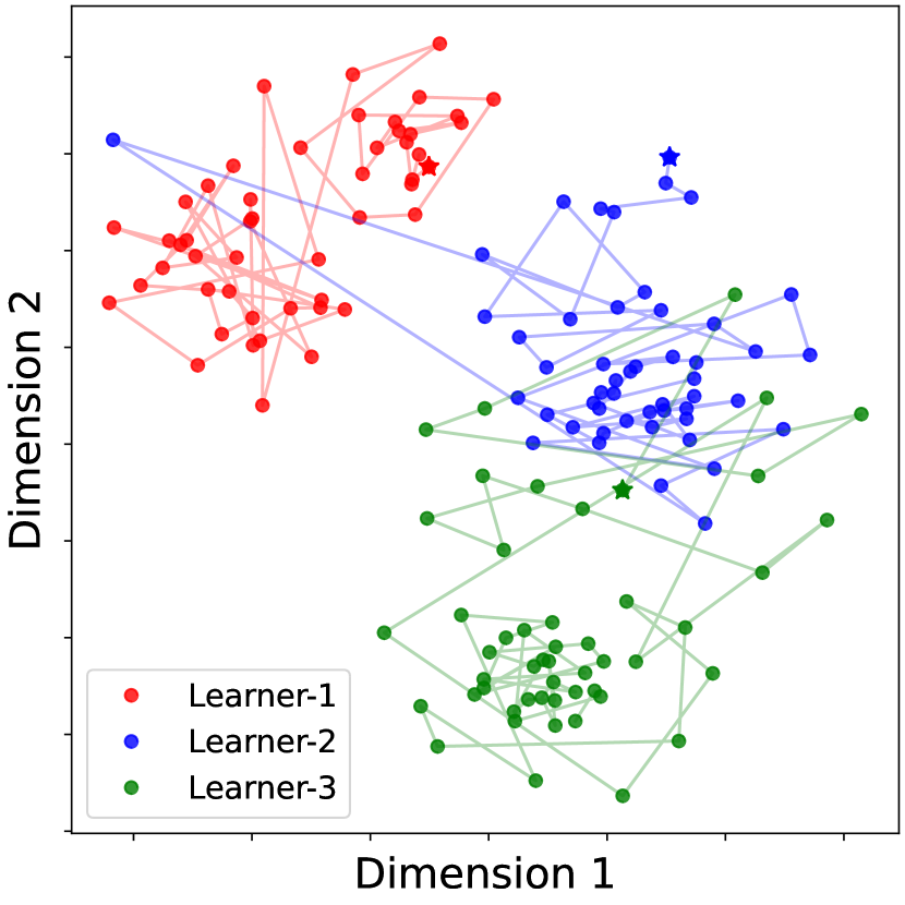
(a) BNN Sequential Ensemble

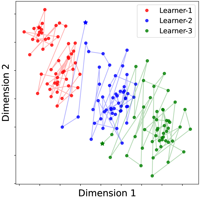
(b) SeBayS-Freeze Ensemble

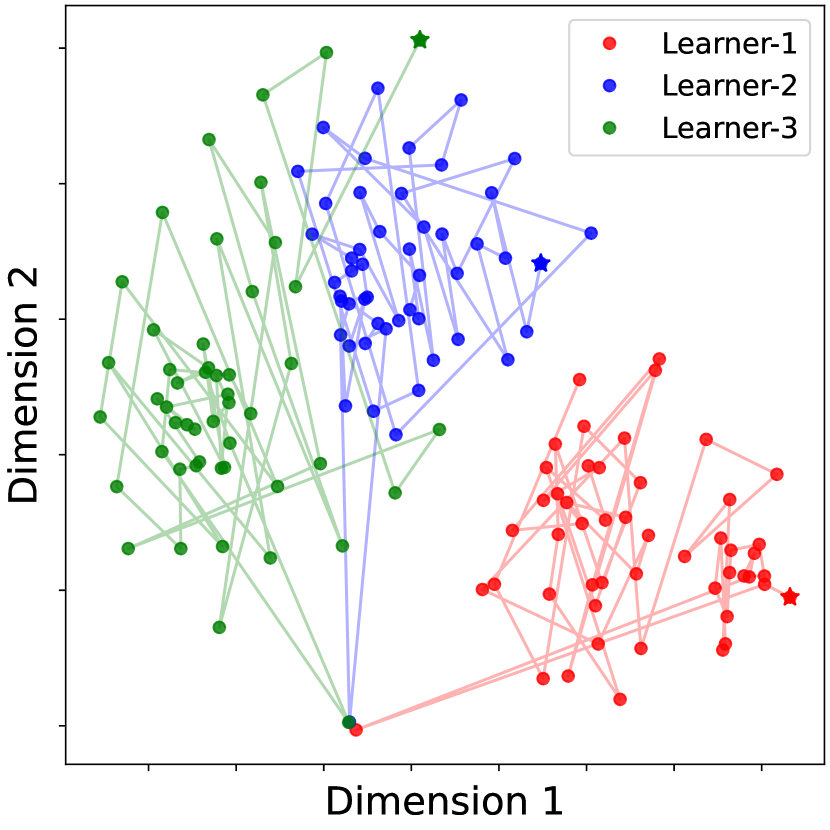
(c) SeBayS-No Freeze Ensemble

Figure 1: Training trajectories of base learners obtained by sequential ensembling of dense BNNs, SeBayS-Freeze Ensemble, and SeBayS-No Freeze Ensemble for ResNet32 on CIFAR10.

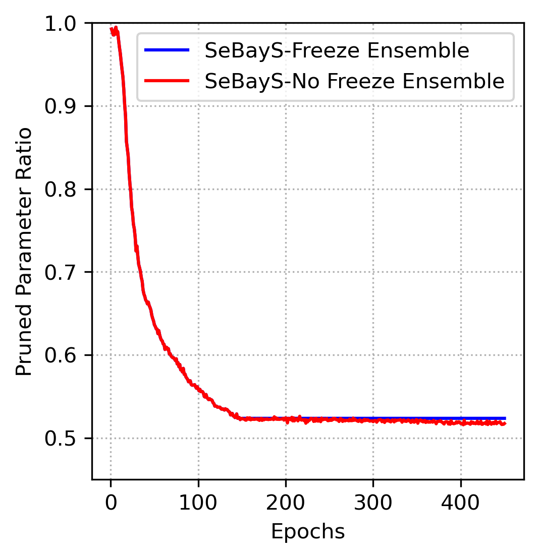
(a) Pruned Parameter Ratio

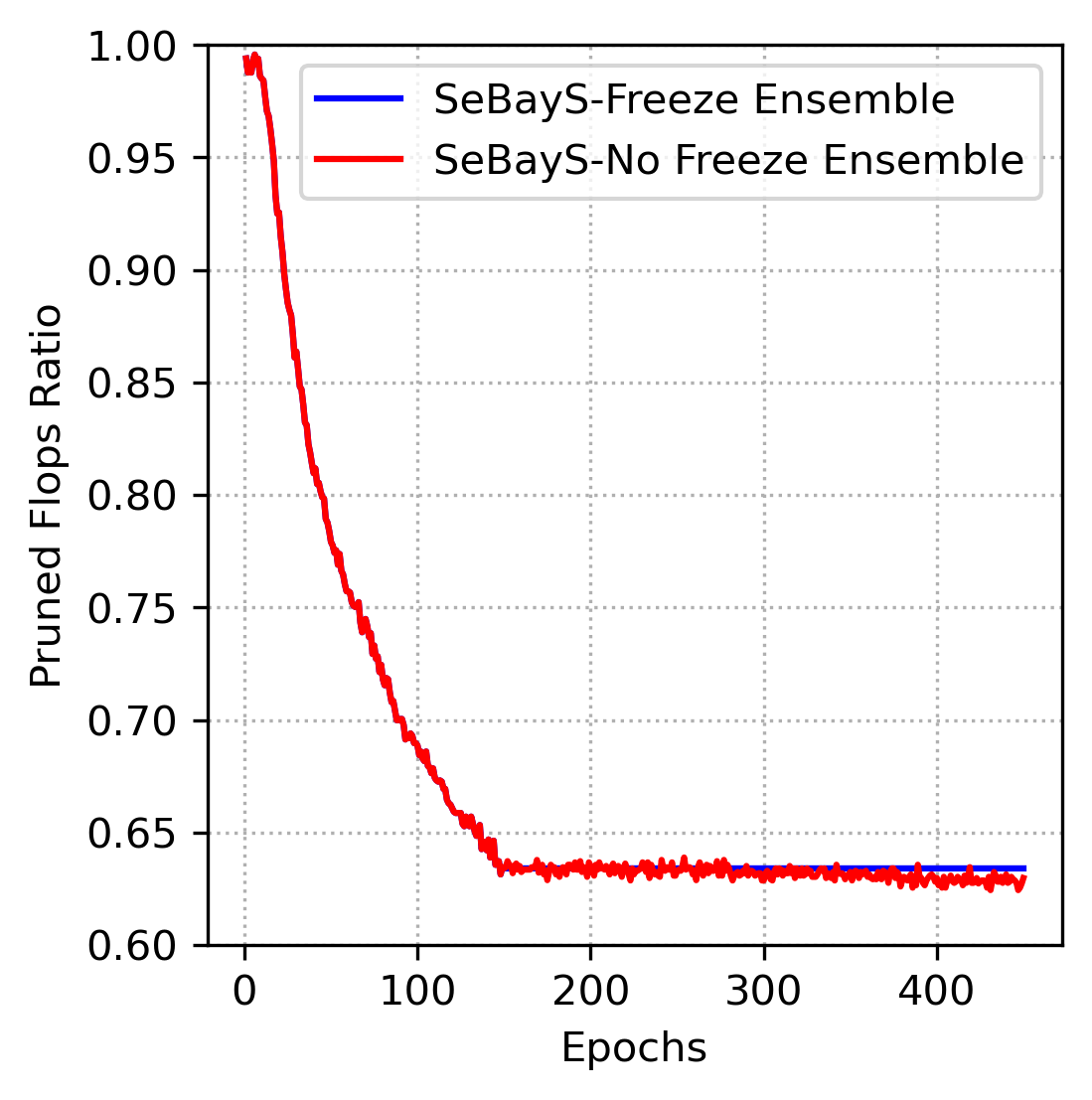
(b) Pruned Flops Ratio

Figure 2: Dynamic sparsity and FLOPs curves showing ratio of remaining parameters and FLOPs in the model for our SeBayS-Freeze and SeBayS-No Freeze ensembles in ResNet32-CIFAR10.

5.2 Dynamic Sparsity Learning

In this section, we highlight the dynamic sparsity training in our SeBayS ensemble methods. We focus on ResNet-32/CIFAR10 experiment and consider $M=3$ exploitation phases. In particular, we plot the ratios of remaining parameters and floating point operations (FLOPs) in the SeBayS sparse base learners. In Figure 2, We observe that during exploration phase, SeBayS prunes off  $50\%$ of the network parameters and more than $35\%$ of the FLOPs compared to its dense counterpart.

5.3 Effect of Ensemble size

In this section, we explore the effect of the ensemble size $M$ in ResNet-32/CIFAR10 experiment. According to the ensembling literature [47, 48], increasing number of diverse base learners in the ensemble improves predictive performance, although with a diminishing impact. In our ensembles, we generate models and aggregate performance sequentially with increasing $M$, the number of base learners in the ensemble.

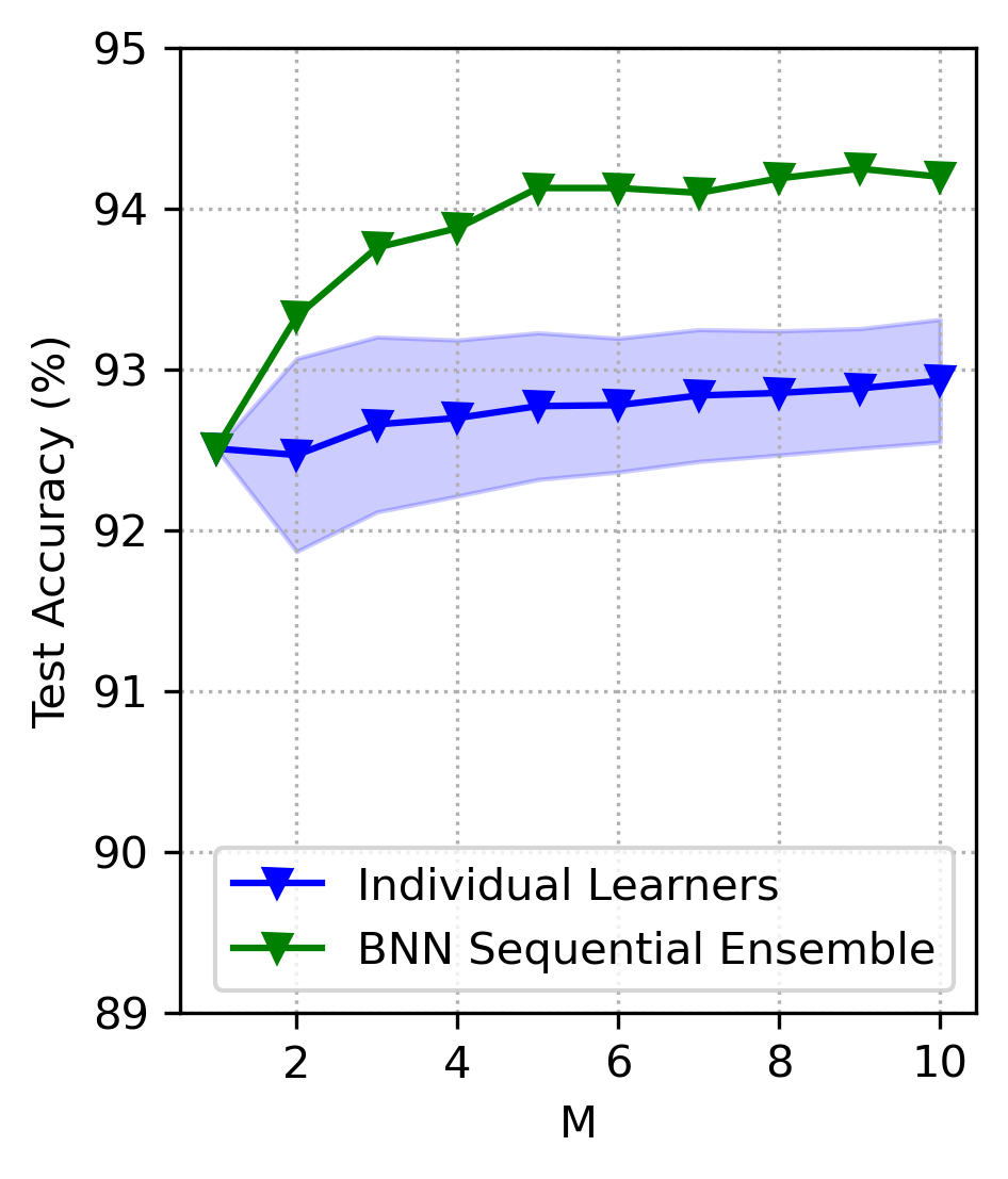
(a) BNN Sequential Ensemble

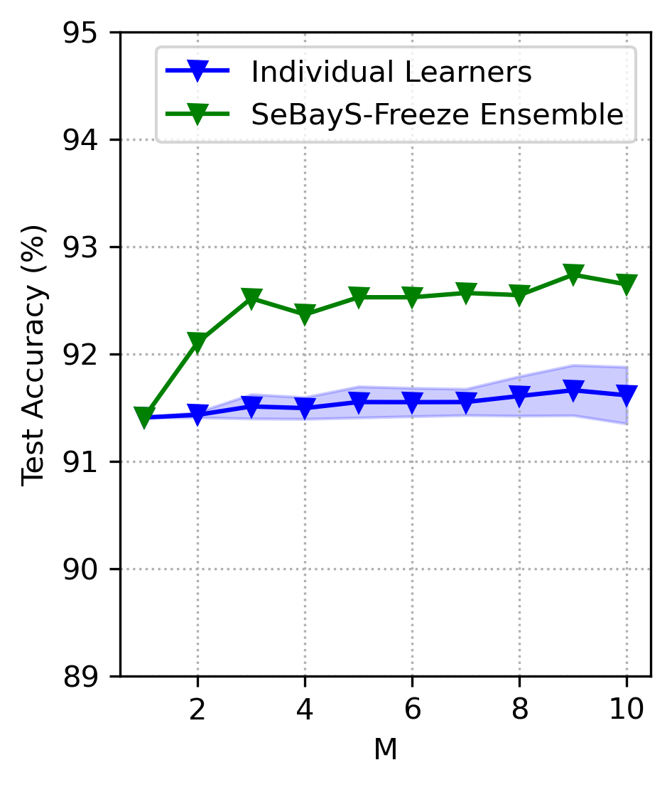
(b) SeBayS-Freeze Ensemble

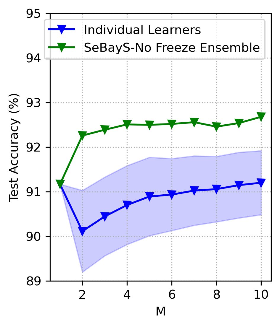
(c) SeBayS-No Freeze Ensemble

Figure 3: Predictive performance of the base learners and the sequential ensembles as the ensemble size M varies for ResNet32 on CIFAR10 experiment.

In Figure 3, we plot the performance of the individual base learners, as well as the sequential ensemble as $M$ varies. For individual learners, we provide the mean test accuracy with corresponding one standard deviation spread. When $M=1$, the ensemble and individual model refer to a single base learner and hence their performance is matched. As $M$ grows, we observe significant increase in the performance of our ensemble models with diminishing improvement for higher $M$s. The high performance of our sequential ensembles compared to their individual base models further underscores the benefits of ensembling in sequential manner.

6 Conclusion and Discussion

In this work, we propose SeBayS ensemble, which is an approach to generate sequential Bayesian neural subnetwork ensembles through a combination of novel sequential ensembling approach for BNNs and dynamic sparsity with sparsity-inducing Bayesian prior that provides a simple and effective approach to improve the predictive performance and model robustness. The highly diverse Bayesian neural subnetworks converge to different optima in function space and, when combined, form an ensemble which demonstrates improving performance with increasing ensemble size. Our simple yet highly effective sequential perturbation strategy enables a dense BNN ensemble to outperform deterministic dense ensemble. Whereas, the Bayesian neural subnetworks obtained using spike-and-slab node pruning prior produce ensembles that are highly diverse, especially the SeBays-No Freeze ensembles compared to EDST in both CIFAR10/100 experiments and DST ensemble in our simpler CIFAR10 experiment. Future work will explore the combination of parallel ensembling of our sequential ensembles leading to a multilevel ensembling model. In particular, we will leverage the exploration phase to reach highly sparse network and next perturb more than once and learn each subnetwork in parallel while performing sequential exploitation phases on each subnetwork. We expect this strategy would lead to highly diverse base learners with potentially significant improvements in model performance and robustness.

Broader Impacts. As deep learning gets harnessed by big industrial corporations in recent years to improve their products, the demand for models with both high predictive and uncertainty estimation performance is rising. Our efficient sequential ensembles provide a compelling approach to yield efficient models with low computational overhead. The Bayesian framework estimates the posterior of model parameters allowing for uncertainty quantification around the parameter estimates which can be vital in medical diagnostics. For example, many of the brain imaging data could be processed through our model yielding a decision regarding certain medical condition with added benefit of quantified confidence associated with that decision. To this end, we do not anticipate any potential negative societal impacts resulting from our work. Moreover, we do not believe there are any ethical concerns applicable to our work.

Appendix A Spike-and-Slab Implementation

The Evidence Lower Bound (ELBO) is represented as

$$\mathcal{L}=-\mathbb{E}_{q(\bm{\theta})}[\log p(\mathcal{D}|\bm{\theta})]+d_{\rm KL}(q(\bm{\theta}),p(\bm{\theta})),$$

where $\mathcal{L}$ in the case of SSBNN [30], which are base learners in our SeBayS ensembles, consists of KL of discrete variables leading to a non-differentiable loss and thus creates a challenge in practical implementation. Instead, [30] apply continuous relaxation, i.e., to approximate discrete random variables by a continuous distribution. Specifically, the continuous relaxation approximation is achieved through Gumbel-softmax (GS) distribution [49], [50], that is $q(z_{lj})\sim{\rm Bernoulli}(\gamma_{lj})$ is approximated by $q(\tilde{z}_{lj})\sim{\rm GS}(\gamma_{lj},\tau)$, where

$$\tilde{z}_{lj}=(1+\exp(-\eta_{lj}/\tau))^{-1},\quad\eta_{lj}=\log(\gamma_{lj}/(1-\gamma_{lj}))+\log(u_{lj}/(1-u_{lj})),\quad u_{lj}\sim{\rm Uniform}(0,1)$$

where $\tau$ is the temperature. We fix the $\tau=0.5$ for all the experiments, similar to [30]. $\tilde{z}_{lj}$ is used in the backward pass for easier gradient calculation, while $z_{lj}$ is used for the exact sparsity in the forward pass.

Appendix B Reproducibility Considerations

B.1 Hyperparameters

Hyperparameters for single and parallel ensemble models. For the ResNet/CIFAR models, we use minibatch size of 128 uniformly across all the methods. We train each single model (Deterministic, BNN, SSBNN) as well as each member of Dense and DST ensemble for 250 epochs with a learning rate of 0.1 which is decayed by a factor of 0.1 at 150 and 200 epochs. For frequentist methods, we use weight decay of $5e-4$ whereas for Bayesian models the weight decay is $0$ (since the KL term in the loss acts as a regularizer). For the DST ensemble, we take the sparsity $S=0.8$, the update interval $\Delta T=1000$, and the exploration rate $p=0.5$, the same as [12].

Hyperparameters for sequential ensemble models. For the ResNet/CIFAR models, the minibatch size is 128 for all the methods compared. We train each sequential model with $M=3$ for 450 epochs. In the BNN and SeBayS ensembles, the exploration phase is run for $t_{0}=150$ epochs and each exploitation phase is run for $t_{\rm ex}=100$ epochs. We fix the perturbation factor to be $3$. During the exploration phase, we take a high learning rate of 0.1. Whereas, for each exploitation phase, we use learning rate of 0.01 for first $t_{\rm ex}/2=50$ epochs and 0.001 for remaining $t_{\rm ex}/2=50$ epochs. For the EDST ensemble, we take an exploration time ($t_{\rm ex}$) of 150 epochs, each refinement phase time ($t_{\rm re}$) of 100 epochs, sparsity $S=0.8$, and exploration rate $q=0.8$, the same as [12].

B.2 Data Augmentation

For CIFAR10 and CIFAR100 training dataset, we first pad the train images using 4 pixels of value 0 on all borders and then crop the padded image at a random location generating train images of the same size as the original train images. Next, with a probability of 0.5, we horizontally flip a given cropped image. Finally, we normalize the images using ${\rm\texttt{mean}}=(0.4914,0.4822,0.4465)$ and ${\rm\texttt{standard deviation}}=(0.2470,0.2435,0.2616)$ for CIFAR10. However, we use ${\rm\texttt{mean}}=(0.5071,0.4865,0.4409)$ and ${\rm\texttt{standard deviation}}=(0.2673,0.2564,0.2762)$ for CIFAR100. Next, we split the train data of size 50000 images into a TRAIN/VALIDATION split of 45000/5000 transformed images. For CIFAR10/100 test data, we normalize the 10000 test images in each data case using the corresponding mean and standard deviation of their respective training data.

B.3 Evaluation Metrics

We quantify the predictive performance of each method using the accuracy of the test (Acc). For a measure of robustness or predictive uncertainty, we use negative log-likelihood (NLL) calculated on the test dataset. Moreover, we adopt {cAcc, cNLL} to denote the corresponding metrics on corrupted test datasets. We also use VALIDATION data to determine the best epoch in each model which is later used for TEST data evaluation.

In the case of Deterministic and each member of Dense, MIMO, and DST ensemble, we use a single prediction for each test data element and calculate the corresponding evaluation metrics for each individual model. In case of all the Bayesian models, we use one Monte Carlo sample to generate the network parameters and correspondingly generate a single prediction for each single model, which is used to calculate the evaluation metrics in those individual models. For all the ensemble models, we generate a single prediction from each base model present in the ensemble. Next, we evaluate the ensemble prediction using a simple average of $M$ predictions generated from $M$ base models and use this averaged prediction to calculate the evaluation metrics mentioned above for the ensemble models.

B.4 Hardware and Software

The Deterministic, MIMO, Rank-1 BNN and Dense Ensemble models are run using the Uncertainty Baselines [44] repository, but with the data, model and hyperparmeter settings described above. Moreover, we consistently run all the experiments on a single NVIDIA A100 GPU for all the approaches evaluated in this work.

Appendix C OOD Experiment Results

In Table 4, we present the AU-ROC results for out-of-distribution (OoD) detection for the ResNet-32/CIFAR10 models. In this case, the out-of-distribution data was taken to be CIFAR100. The results show that our SebayS-Freeze Ensemble perform better than the single SSBNN and MIMO model. whereas, SebayS-No Freeze Ensemble performss better than SSBNN. Next, our BNN sequential ensemble performs better than deterministic and BNN models.

Table 4: ResNet-32/CIFAR10 experiment results For OoD Detection: we mark the best results out of single-pass sparse models in bold and single-pass dense models in blue.

Methods	AUROC ($\uparrow$)	# Forward passes ($\downarrow$)
SSBNN	0.806	1
MIMO (M=3)	0.842	1
EDST Ensemble (M = 3)	0.872	1
SeBayS-Freeze Ensemble (M = 3)	0.864	1
SeBayS-No Freeze Ensemble (M = 3)	0.842	1
DST Ensemble (M = 3)	0.879	3
Deterministic	0.848	1
BNN	0.841	1
Rank-1 BNN (M=3)	0.866	1
BNN Sequential Ensemble (M = 3)	0.863	1
Dense Ensemble (M=3)	0.878	3

Appendix D Effect of the Ensemble Size

In Section 5.3, we have explored the effect of the ensemble size $M$ in ResNet-32/CIFAR10 experiment through comparison of mean individual learner test accuracies compared to ensemble accuracies in uncorrupted test dataset. In this Appendix, we provide the results on both CIFAR10 and CIFAR10-C datasets for our sequential ensembles with an increasing number of base learners $M=3,5,10$. We also provide BNN and SSBNN baselines to compare against BNN sequential ensemble and SeBayS ensembles, respectively. We observe that our BNN sequential ensemble and SeBayS ensembles of any size significantly outperform single BNN and SSBNN models, respectively. With an increasing number of base learners ($M=3,5,10$) within each of our sequential ensembles, we observe a monotonically increasing predictive performance. The NLLs for BNN sequential ensemble decrease as $M$ increases. The NLLs for the SeBayS ensembles are either similar or increasing as $M$ increases, which suggests the influence of the KL divergence term in ELBO optimization in variational inference.

Table 5: ResNet-32/CIFAR10 experiment results: we mark the best results out of the sparse models in bold and the dense models in blue.

Methods	Acc ($\uparrow$)	NLL ($\downarrow$)		cAcc ($\uparrow$)	cNLL ($\downarrow$)		# Forward passes ($\downarrow$)
SSBNN	91.2	0.320		67.5	1.479		1
SeBayS-Freeze Ensemble (M = 3)	92.5	0.273		70.4	1.344		1
SeBayS-Freeze Ensemble (M = 5)	92.5	0.273		70.9	1.359		1
SeBayS-Freeze Ensemble (M = 10)	92.7	0.275		71.0	1.386		1
SeBayS-No Freeze Ensemble (M = 3)	92.4	0.274		69.8	1.356		1
SeBayS-No Freeze Ensemble (M = 5)	92.5	0.271		70.2	1.375		1
SeBayS-No Freeze Ensemble (M = 10)	92.7	0.272		70.8	1.375		1
BNN	91.9	0.353		71.3	1.422		1
BNN Sequential Ensemble (M = 3)	93.8	0.265		73.3	1.341		1
BNN Sequential Ensemble (M = 5)	94.1	0.253		73.7	1.318		1
BNN Sequential Ensemble (M = 10)	94.2	0.244		73.9	1.300		1

Appendix E Effect of the Monte Carlo Sample Size

In variational inference during evaluation phase, model prediction is calculated using the average of the predictions from ensemble of networks where the weights of each network represent one sample from the posterior distributions of the weights. The number of such networks used to build ensemble prediction is called the Monte Carlo ($MC$) sample. In Table 6, we present our sequential ensemble models as well as BNN and SSBNN baselines in the ResNet-32 / CIFAR10 experiment. Here, we take $MC=1$ which is used in the main paper and compare it with $MC=5$ for each method. In single BNN and SSBNN models, we observe significant improvement in model performance when using $MC=5$ instead of $1$. However, when we compare the SebayS ensembles using $MC=1$ or $5$ with SSBNN using $MC=5$, we observe that their performance is similar, indicating that $MC=1$ is sufficient for our SebayS ensembles. On the other hand, sequential BNN ensembles using $MC=1$ has better performance compared to BNN with $MC=5$. Whereas, sequential BNN ensemble using $MC=1$ and $5$ have similar performance. This highlights the importance of sequential perturbation strategy, which leads to more diverse ensembles compared to mere Monte Carlo sampling.

Table 6: ResNet-32/CIFAR10 experiment results: we mark the best results out of the sparse models in bold and dense models in blue. $MC$ is the Monte Carlo sample size

Methods	$MC$	Acc ($\uparrow$)	NLL ($\downarrow$)
SSBNN	1	91.2	0.320
SSBNN	5	92.3	0.270
SeBayS-Freeze Ensemble (M=3)	1	92.5	0.273
SeBayS-Freeze Ensemble (M=3)	5	92.5	0.270
SeBayS-No Freeze Ensemble (M=3)	1	92.4	0.274
SeBayS-No Freeze Ensemble (M=3)	5	92.6	0.268
BNN	1	91.9	0.353
BNN	5	93.2	0.271
BNN Sequential Ensemble (M=3)	1	93.8	0.265
BNN Sequential Ensemble (M=3)	5	93.9	0.254

Appendix F Effect of the Perturbation Factor

In this Appendix, we explore the influence of the perturbation factor on our sequential ensemble models through the ResNet-32/CIFAR10 experiment. In Table 7, we report the results for our three sequential approaches for three perturbation factors, $\rho=2,3,5$. For our SeBayS-Freeze and No Freeze ensembles, the lower perturbations with $\rho=2$ lead to higher test accuracies and NLLs over $\rho=3,5$ in both the CIFAR10 and CIFAR10-C test datasets. This means that higher perturbations $\rho=3,5$ might need a higher number of epochs to reach the convergence in each exploitation phase. However, in the BNN sequential ensemble $\rho=3$ has an overall higher performance compared to $\rho=2,5$. This points to the fact that the lower perturbation, $\rho=2$, may not lead to the best ensemble model. In Table 8, we present the prediction disagreement and KL divergence metrics for the experiments described in this Appendix. In the BNN sequential ensemble, the $\rho=5$ perturbation model has the best diversity metrics, whereas the $\rho=3$ perturbation model has the best accuracy. In the SeBayS approach, the perturbation of $\rho=3$ leads to the best diversity metrics nonetheless at the expense of slightly lower predictive performance. This highlights the fact that the $\rho=3$ SeBayS approaches lead to the best ensembles given the training budget constraint. Hence, we use $\rho=3$ for our three sequential models in all the experiments presented in the main paper.

Table 7: ResNet-32/CIFAR10 experiment results: we mark the best results out of different perturbation models under a given method in bold. Ensemble size is fixed at $M=3$. $\rho$ is the perturbation factor.

Methods	$\rho$	Acc ($\uparrow$)	NLL ($\downarrow$)		cAcc ($\uparrow$)	cNLL ($\downarrow$)
SeBayS-Freeze Ensemble	2	92.7	0.264		70.6	1.303
SeBayS-Freeze Ensemble	3	92.5	0.273		70.4	1.344
SeBayS-Freeze Ensemble	5	92.5	0.267		70.6	1.314
SeBayS-No Freeze Ensemble	2	92.7	0.268		70.4	1.331
SeBayS-No Freeze Ensemble	3	92.4	0.274		69.8	1.356
SeBayS-No Freeze Ensemble	5	92.4	0.272		70.1	1.353
BNN Sequential Ensemble	2	93.6	0.269		73.3	1.361
BNN Sequential Ensemble	3	93.8	0.265		73.3	1.341
BNN Sequential Ensemble	5	93.6	0.262		73.0	1.366

Table 8: Diversity metrics: prediction disagreement $(d_{\rm dis})$ and KL divergence $(d_{\rm KL})$. We mark the best results out of different perturbation models under a given method in bold. Ensemble size is fixed at $M=3$. $\rho$ is the perturbation factor.

		ResNet-32/CIFAR10
Methods	$\rho$	$(d_{\rm dis})$ ($\uparrow$)	$d_{\rm KL}$ ($\uparrow$)	Acc ($\uparrow$)
BNN Sequential Ensemble	2	0.062	0.205	93.6
BNN Sequential Ensemble	3	0.061	0.201	93.8
BNN Sequential Ensemble	5	0.063	0.211	93.6
SeBayS-Freeze Ensemble	2	0.058	0.135	92.7
SeBayS-Freeze Ensemble	3	0.060	0.138	92.5
SeBayS-Freeze Ensemble	5	0.059	0.137	92.5
SeBayS-No Freeze Ensemble	2	0.082	0.222	92.7
SeBayS-No Freeze Ensemble	3	0.106	0.346	92.4
SeBayS-No Freeze Ensemble	5	0.083	0.228	92.4

Appendix G Effect of the Cyclic Learning Rate Schedule

In this Appendix, we provide the effect of different cyclic learning rate strategies during exploitation phases in our three sequential ensemble methods. We explore the stepwise (our approach), cosine [8], linear-fge [20], and linear-1 cyclic learning rate schedules.

Cosine. The cyclic cosine learning rate schedule reduces the higher learning rate of 0.01 to a lower learning rate of 0.001 using the shifted cosine function [8] in each exploitation phase.

Linear-fge. In the cyclic linear-fge learning rate schedule, we first drop the high learning rate of 0.1 used in the exploration phase to 0.01 linearly in ${\rm t_{ex}}/2$ epochs and then further drop the learning rate to 0.001 linearly for the remaining ${\rm t_{ex}}/2$ epochs during the first exploitation phase. Afterwards, in each exploitation phase, we linearly increase the learning rate from 0.001 to 0.01 for ${\rm t_{ex}}/2$ and then linearly decrease it back to 0.001 for the next ${\rm t_{ex}}/2$ similar to [20].

Linear-1. In the linear-1 cyclic learning rate schedule, we linearly decrease the learning rate from 0.01 to 0.001 for ${\rm t_{ex}}$ epochs in each exploitation phase and then suddenly increase the learning to 0.01 after each sequential perturbation step.

In Figure 4, we present the plots of the cyclic learning rate schedules considered in this Appendix.

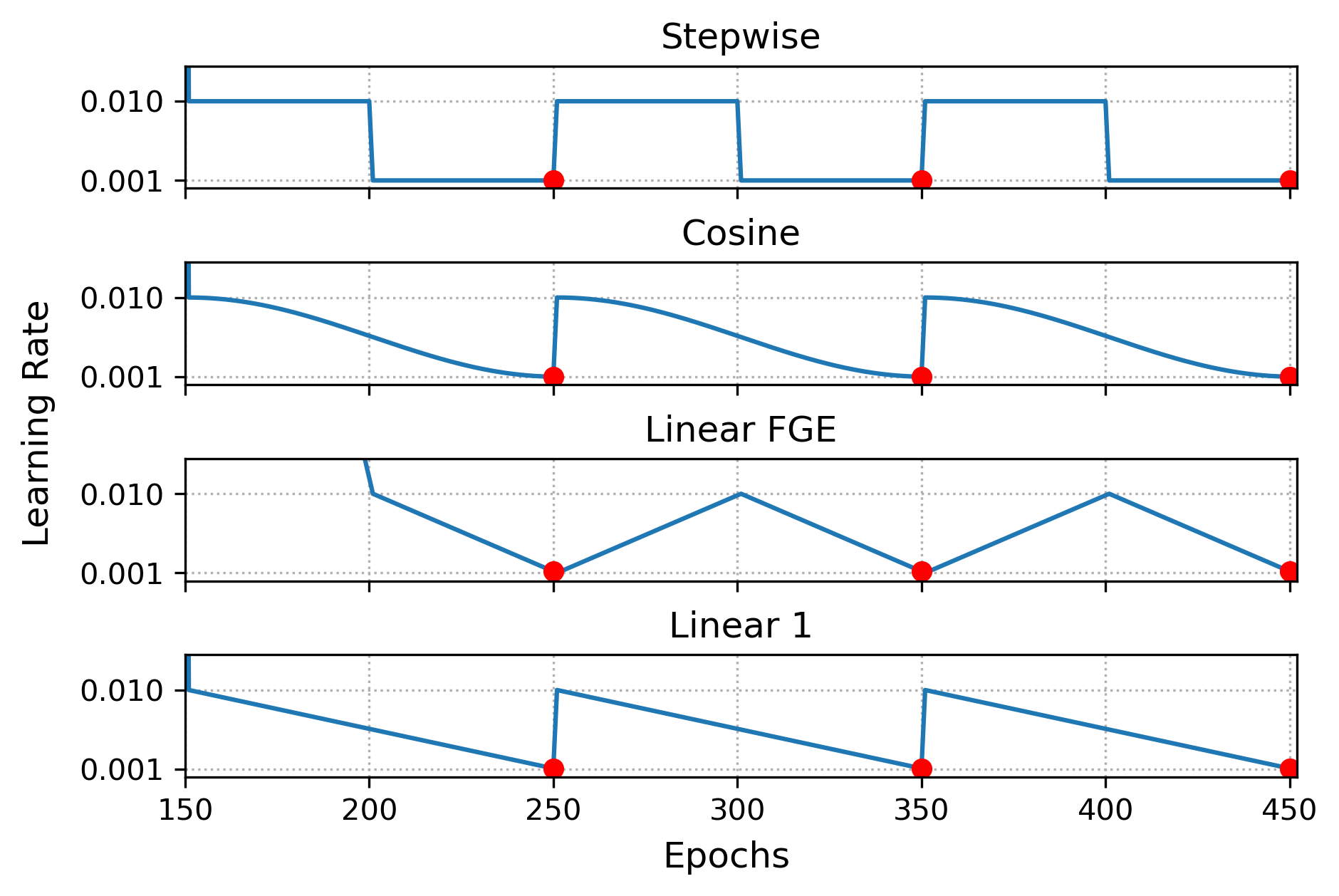
Figure 4: Cyclic Learning Rate Schedules. The red dots represent the converged models after each exploitation phase used in our final sequential ensemble.

In Table 9, we present the results for our three sequential ensemble methods under the four cyclic learning rate schedules mentioned above. We observe that, in all three sequential ensembles, the cyclic stepwise learning rate schedule yields the best performance in almost all criteria compared to the rest of the learning rate schedules in each sequential ensemble method. In Table 10, we present the prediction disagreement and KL divergence metrics for the experiments described in this Appendix. We observe that, in SeBayS-No Freeze ensemble, cyclic stepwise schedule generates highly diverse subnetworks, which also leads to high predictive performance. Whereas, in the BNN sequential and SeBayS-Freeze ensemble, we observe lower diversity metrics for the cyclic stepwise learning rate schedule compared to the rest of the learning rate schedules.

Table 9: ResNet-32/CIFAR10 experiment results: we mark the best results out of different learning rate (LR) schedules under a given method in bold. Ensemble size is fixed at $M=3$.

Methods	LR Schedule	Acc ($\uparrow$)	NLL ($\downarrow$)		cAcc ($\uparrow$)	cNLL ($\downarrow$)
SeBayS-Freeze Ensemble	stepwise	92.5	0.273		70.4	1.344
SeBayS-Freeze Ensemble	cosine	92.3	0.301		69.8	1.462
SeBayS-Freeze Ensemble	linear-fge	92.5	0.270		70.1	1.363
SeBayS-Freeze Ensemble	linear-1	92.1	0.310		69.8	1.454
SeBayS-No Freeze Ensemble	stepwise	92.4	0.274		69.8	1.356
SeBayS-No Freeze Ensemble	cosine	92.2	0.294		69.9	1.403
SeBayS-No Freeze Ensemble	linear-fge	92.4	0.276		70.0	1.379
SeBayS-No Freeze Ensemble	linear-1	92.2	0.296		69.7	1.412
BNN Sequential Ensemble	stepwise	93.8	0.265		73.3	1.341
BNN Sequential Ensemble	cosine	93.7	0.279		72.7	1.440
BNN Sequential Ensemble	linear-fge	93.5	0.270		73.1	1.342
BNN Sequential Ensemble	linear-1	93.4	0.287		72.2	1.430

Table 10: Diversity metrics: prediction disagreement $(d_{\rm dis})$ and KL divergence $(d_{\rm KL})$. We mark the best results out of different learning rate (LR) schedules under a given method in bold. Ensemble size is fixed at $M=3$.

		ResNet-32/CIFAR10
Methods	LR Schedule	$(d_{\rm dis})$ ($\uparrow$)	$d_{\rm KL}$ ($\uparrow$)	Acc ($\uparrow$)
BNN Sequential Ensemble	stepwise	0.061	0.201	93.8
BNN Sequential Ensemble	cosine	0.068	0.256	93.7
BNN Sequential Ensemble	linear-fge	0.070	0.249	93.5
BNN Sequential Ensemble	linear-1	0.071	0.275	93.4
SeBayS-Freeze Ensemble	stepwise	0.060	0.138	92.5
SeBayS-Freeze Ensemble	cosine	0.072	0.204	92.3
SeBayS-Freeze Ensemble	linear-fge	0.076	0.215	92.5
SeBayS-Freeze Ensemble	linear-1	0.074	0.209	92.1
SeBayS-No Freeze Ensemble	stepwise	0.106	0.346	92.4
SeBayS-No Freeze Ensemble	cosine	0.078	0.222	92.2
SeBayS-No Freeze Ensemble	linear-fge	0.074	0.199	92.4
SeBayS-No Freeze Ensemble	linear-1	0.077	0.217	92.2

References

- LeCun et al. [2015] LeCun, Y., Bengio, Y., and Hinton, G. (2015), “Deep learning,” Nature, 521, 436–444.
- Bartlett et al. [2021] Bartlett, P. L., Montanari, A., and Rakhlin, A. (2021), “Deep learning: a statistical viewpoint,” Acta Numerica, 30, 87–201.
- Wicker et al. [2021] Wicker, M., Laurenti, L., Patane, A., Chen, Z., Zhang, Z., and Kwiatkowska, M. (2021), “Bayesian inference with certifiable adversarial robustness,” in International Conference on Artificial Intelligence and Statistics, pp. 2431–2439, PMLR.
- Jordan et al. [1999] Jordan, M. I., Ghahramani, Z., Jaakkola, T. S., and Sau, L. K. (1999), “An Introduction to Variational Methods for Graphical Models,” Machine Learning, 37, 183–233.
- Izmailov et al. [2021] Izmailov, P., Vikram, S., Hoffman, M. D., and Wilson, A. G. G. (2021), “What Are Bayesian Neural Network Posteriors Really Like?” in Proceedings of the 38th International Conference on Machine Learning (ICML-2021), pp. 4629–4640.
- Lakshminarayanan et al. [2017] Lakshminarayanan, B., Pritzel, A., and Blundell, C. (2017), “Simple and scalable predictive uncertainty estimation using deep ensembles,” Advances in neural information processing systems, 30.
- Wilson and Izmailov [2020] Wilson, A. G. and Izmailov, P. (2020), “Bayesian deep learning and a probabilistic perspective of generalization,” Advances in neural information processing systems, 33, 4697–4708.
- Huang et al. [2017] Huang, G., Li, Y., Pleiss, G., Liu, Z., Hopcroft, J. E., and Weinberger, K. Q. (2017), “Snapshot ensembles: Train 1, get m for free,” in International Conference on Learning Representations (ICLR 2017).
- D’Angelo and Fortuin [2021] D’Angelo, F. and Fortuin, V. (2021), “Repulsive deep ensembles are Bayesian,” Advances in Neural Information Processing Systems, 34.
- Dusenberry et al. [2020] Dusenberry, M., Jerfel, G., Wen, Y., Ma, Y., Snoek, J., Heller, K., Lakshminarayanan, B., and Tran, D. (2020), “Efficient and Scalable Bayesian Neural Nets with Rank-1 Factors,” in Proceedings of the 37th International Conference on Machine Learning (ICML-2020).
- Havasi et al. [2021] Havasi, M., Jenatton, R., Fort, S., Liu, J. Z., Snoek, J., Lakshminarayanan, B., Dai, A. M., and Tran, D. (2021), “Training independent subnetworks for robust prediction,” in 9th International Conference on Learning Representations (ICLR-2021).
- Liu et al. [2022] Liu, S., Chen, T., Atashgahi, Z., Chen, X., Sokar, G., Mocanu, E., Pechenizkiy, M., Wang, Z., and Mocanu, D. C. (2022), “Deep Ensembling with No Overhead for either Training or Testing: The All-Round Blessings of Dynamic Sparsity,” in 10th International Conference on Learning Representations (ICLR-2022).
- Egele et al. [2021] Egele, R., Maulik, R., Raghavan, K., Balaprakash, P., and Lusch, B. (2021), “AutoDEUQ: Automated Deep Ensemble with Uncertainty Quantification,” arXiv preprint arXiv:2110.13511.
- Wenzel et al. [2020] Wenzel, F., Snoek, J., Tran, D., and Jenatton, R. (2020), “Hyperparameter ensembles for robustness and uncertainty quantification,” Advances in Neural Information Processing Systems, 33, 6514–6527.
- Swann and Allinson [1998] Swann, A. and Allinson, N. (1998), “Fast committee learning: Preliminary results,” Electronics Letters, 34, 1408–1410.
- Xie et al. [2013] Xie, J., Xu, B., and Chuang, Z. (2013), “Horizontal and vertical ensemble with deep representation for classification,” arXiv preprint arXiv:1306.2759.
- Jean et al. [2015] Jean, S., Cho, K., Memisevic, R., and Bengio, Y. (2015), “On using very large target vocabulary for neural machine translation,” in Proceedings of the 53rd Annual Meeting of the Association for Computational Linguistics and the 7th International Joint Conference on Natural Language Processing (Volume 1: Long Papers), pp. 1–10.
- Sennrich et al. [2016] Sennrich, R., Haddow, B., and Birch, A. (2016), “Edinburgh neural machine translation systems for WMT 16,” arXiv preprint arXiv:1606.02891.
- Moghimi et al. [2016] Moghimi, M., Belongie, S. J., Saberian, M. J., Yang, J., Vasconcelos, N., and Li, L.-J. (2016), “Boosted convolutional neural networks,” in BMVC, vol. 5, p. 6.
- Garipov et al. [2018] Garipov, T., Izmailov, P., Podoprikhin, D., Vetrov, D. P., and Wilson, A. G. (2018), “Loss Surfaces, Mode Connectivity, and Fast Ensembling of DNNs,” in Advances in Neural Information Processing Systems (NeurIPS-2018), vol. 31.
- Hoefler et al. [2021] Hoefler, T., Alistarh, D., Ben-Nun, T., Dryden, N., and Peste, A. (2021), “Sparsity in Deep Learning: Pruning and growth for efficient inference and training in neural networks,” Journal of Machine Learning Research, 22, 1–124.
- Frankle and Carbin [2019] Frankle, J. and Carbin, M. (2019), “The Lottery Ticket Hypothesis: Finding Sparse, Trainable Neural Networks,” in International Conference on Learning Representations (ICLR 2019), New Orleans, USA.
- Han et al. [2016] Han, S., Mao, H., and Dally, W. J. (2016), “Deep Compression: Compressing Deep Neural Network with Pruning, Trained Quantization and Huffman Coding,” in 4th International Conference on Learning Representations (ICLR-2016), San Juan, Puerto Rico.
- Molchanov et al. [2017] Molchanov, D., Ashukha, A., and Vetrov, D. (2017), “Variational Dropout Sparsifies Deep Neural Networks,” in Proceedings of the 34th International Conference on Machine Learning (ICML-2027), vol. 70, p. 2498–2507, Sydney, NSW, Australia.
- Wen et al. [2016] Wen, W., Wu, C., Wang, Y., Chen, Y., and Li, H. (2016), “Learning Structured Sparsity in Deep Neural Networks,” in Proceedings of the 29th Advances in Neural Information Processing Systems (NIPS 2016), Barcelona, Spain.
- Robert et al. [2007] Robert, C. P. et al. (2007), The Bayesian choice: from decision-theoretic foundations to computational implementation, vol. 2, Springer.
- Bai et al. [2020] Bai, J., Song, Q., and Cheng, G. (2020), “Efficient Variational Inference for Sparse Deep Learning with Theoretical Guarantee,” in Proceedings of the 34th Advances in Neural Information Processing Systems (NeurIPS 2020), pp. 466–476, Vancouver, Canada.
- Louizos et al. [2017] Louizos, C., Ullrich, K., and Welling, M. (2017), “Bayesian Compression for Deep Learning,” in Proceedings of the 30th Advances in Neural Information Processing Systems (NIPS 2020), pp. 3288–3298, Long Beach, CA, USA.
- Ghosh et al. [2019] Ghosh, S., Yao, J., and Doshi-Velez, F. (2019), “Model Selection in Bayesian Neural Networks via Horseshoe Priors,” Journal of Machine Learning Research, pp. 1–46.
- Jantre et al. [2022] Jantre, S., Bhattacharya, S., and Maiti, T. (2022), “Layer Adaptive Node Selection in Bayesian Neural Networks: Statistical Guarantees and Implementation Details,” arXiv:2108.11000.
- Gal and Ghahramani [2016] Gal, Y. and Ghahramani, Z. (2016), “Dropout as a bayesian approximation: Representing model uncertainty in deep learning,” in international conference on machine learning, pp. 1050–1059, PMLR.
- Wan et al. [2013] Wan, L., Zeiler, M., Zhang, S., Le Cun, Y., and Fergus, R. (2013), “Regularization of neural networks using dropconnect,” in International conference on machine learning, pp. 1058–1066, PMLR.
- Singh et al. [2016] Singh, S., Hoiem, D., and Forsyth, D. (2016), “Swapout: Learning an ensemble of deep architectures,” Advances in neural information processing systems, 29.
- Wen et al. [2020] Wen, Y., Tran, D., and Ba, J. (2020), “Batchensemble: an alternative approach to efficient ensemble and lifelong learning,” arXiv preprint arXiv:2002.06715.
- Blei et al. [2017] Blei, D. M., Kucukelbir, A., and McAuliffe, J. D. (2017), “Variational Inference: A Review for Statisticians,” Journal of the American Statistical Association, 112, 859–877.
- Kingma and Welling [2014] Kingma, D. and Welling, M. (2014), “Auto-Encoding Variational Bayes,” arXiv:1312.6114.
- Mackay [1992] Mackay, D. J. C. (1992), “A practical Bayesian framework for backpropagation networks,” Neural Computation, 4, 448–472.
- Neal [1996] Neal, R. M. (1996), Bayesian Learning for Neural Networks, New York: Springer Verlag.
- Blundell et al. [2015] Blundell, C., Cornebise, J., Kavukcuoglu, K., and Wierstra, D. (2015), “Weight Uncertainty in Neural Network,” in Proceedings of Machine Learning Research, vol. 37, pp. 1613–1622, PMLR.
- Mitchell and Beauchamp [1988] Mitchell, T. J. and Beauchamp, J. J. (1988), “Bayesian Variable Selection in Linear Regression,” Journal of the American Statistical Association, 83, 1023–1032.
- He et al. [2015] He, K., Zhang, X., Ren, S., and Sun, J. (2015), “Delving Deep into Rectifiers: Surpassing Human-Level Performance on ImageNet Classification,” in IEEE International Conference on Computer Vision (ICCV-2015), pp. 1026–1034.
- Sutskever et al. [2013] Sutskever, I., Martens, J., Dahl, G., and Hinton, G. (2013), “On the importance of initialization and momentum in deep learning,” in Proceedings of the 30th International Conference on Machine Learning (ICML-2013), vol. 28, pp. 1139–1147.
- He et al. [2016] He, K., Zhang, X., Ren, S., and Sun, J. (2016), “Deep Residual Learning for Image Recognition,” in IEEE Conference on Computer Vision and Pattern Recognition (CVPR-2016), pp. 770–778.
- Nado et al. [2021] Nado, Z., Band, N., Collier, M., Djolonga, J., Dusenberry, M., Farquhar, S., Filos, A., Havasi, M., Jenatton, R., Jerfel, G., Liu, J., Mariet, Z., Nixon, J., Padhy, S., Ren, J., Rudner, T., Wen, Y., Wenzel, F., Murphy, K., Sculley, D., Lakshminarayanan, B., Snoek, J., Gal, Y., and Tran, D. (2021), “Uncertainty Baselines: Benchmarks for Uncertainty & Robustness in Deep Learning,” arXiv preprint arXiv:2106.04015.
- Hendrycks and Dietterich [2019] Hendrycks, D. and Dietterich, T. (2019), “Benchmarking neural network robustness to common corruptions and perturbations,” in 7th International Conference on Learning Representations (ICLR-2019).
- Van der Maaten and Hinton [2008] Van der Maaten, L. and Hinton, G. (2008), “Visualizing Data using t-SNE,” Journal of Machine Learning Research, 9, 2579–2605.
- Hansen and Salamon [1990] Hansen, L. and Salamon, P. (1990), “Neural network ensembles,” IEEE Transactions on Pattern Analysis and Machine Intelligence, 12, 993–1001.
- Ovadia et al. [2019] Ovadia, Y., Fertig, E., Ren, J., Nado, Z., Sculley, D., Dillon, J. V., Lakshminarayanan, B., and Snoek, J. (2019), “Can you trust your model’s uncertainty? Evaluating predictive uncertainty under dataset shift,” in 32th Advances in Neural Information Processing Systems (NeurIPS-2019), pp. 13969–13980.
- Jang et al. [2017] Jang, E., Gu, S., and Poole, B. (2017), “Categorical Reparameterization with Gumbel-Softmax,” in 5th International Conference on Learning Representations (ICLR 2017), Toulon, France.
- Maddison et al. [2017] Maddison, C. J., Mnih, A., and Teh, Y. W. (2017), “The Concrete Distribution: A Continuous Relaxation of Discrete Random Variables,” in 5th International Conference on Learning Representations (ICLR 2017), Toulon, France.