Efficient Self-supervised Vision Pretraining with Local Masked Reconstruction

Abstract

Self-supervised learning for computer vision has achieved tremendous progress and improved many downstream vision tasks such as image classification, semantic segmentation, and object detection. Among these, generative self-supervised vision learning approaches such as MAE and BEiT show promising performance. However, their global masked reconstruction mechanism is computationally demanding. To address this issue, we propose local masked reconstruction (LoMaR), a simple yet effective approach that performs masked reconstruction within a small window of 7$\times$7 patches on a simple Transformer encoder, improving the trade-off between efficiency and accuracy compared to global masked reconstruction over the entire image. Extensive experiments show that LoMaR reaches 84.1% top-1 accuracy on ImageNet-1K classification, outperforming MAE by 0.5%. After finetuning the pretrained LoMaR on 384$\times$384 images, it can reach 85.4% top-1 accuracy, surpassing MAE by 0.6%. On MS COCO, LoMaR outperforms MAE by 0.5 $\text{AP}^{\text{box}}$ on object detection and 0.5 $\text{AP}^{\text{mask}}$ on instance segmentation. LoMaR is especially more computation-efficient on pretraining high-resolution images, e.g., it is 3.1$\times$ faster than MAE with 0.2% higher classification accuracy on pretraining 448$\times$448 images. This local masked reconstruction learning mechanism can be easily integrated into any other generative self-supervised learning approach. Our code is publicly available in https://github.com/junchen14/LoMaR.

1 Introduction

Recently, self-supervised learning approaches [14, 7, 2, 24, 9, 1, 56, 41, 28] have achieved enormous success in learning representations conducive to downstream applications, such as image classification and object detection. Among these, several generative self-supervised learning methods such as Masked Autoencoder (MAE) [24] and Bidirectional Encoder Representation from Image Transformers (BEiT) [2], which reconstruct the input image from a small portion of image patches, have demonstrated excellent performance.

However, a major bottleneck of current generative self-supervised learning aproaches like MAE and BEiT is their high demand for compute, as they have global masked reconstruction and operate on a large number of image patches. For example, pretraining a MAE-Huge [24] on the 1.2 million images of ImageNet under 224 $\times$ 224 resolution takes 34.5 hours on 128 TPU-v3 GPUs. BEiT[2] training is slower due to the cost associated with the discrete variational autoencoder. High-resolution images further exacerbate this issue. For example, pretraining MAE on 384$\times$384 images consumes 4.7 times the compute time of 224$\times$224 counterpart. However, high-resolution images are essential in many tasks, such as object detection. Thus, improving the efficiency of pretraining holds the promise to unleash additional performance gains under pretraining with a much larger dataset or higher-resolution images.

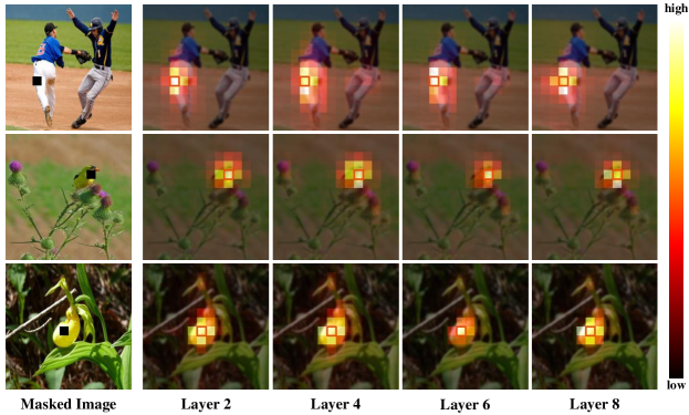
Figure 1: We visualize the attention patterns employed by $\text{MAE}_{\text{Large}}$ [24] in the reconstruction of a random target patch, indicated by orange. Patches that are important for prediction are usually close to the target patch. We selected the images randomly from the ImageNet-1K [16] Val set.

In the Transformer model, the global self-attention mechanism attends to all $n$ image patches, incurring $\mathcal{O}(n^{2})$ time complexity. But the benefits of attending to far-away patches in reconstruction remain unclear. In Fig. 1, we visualize the attention weights when reconstructing a masked image patch (shown in black). From a pretrained $\text{MAE}_{\text{Large}}$ model, we extract the attention weights from the decoder layers 2, 4, 6, and 8 and use white to indicate high attention. The model mostly attends to patches close to the target patch, which motivates us to limit the range of attention used in the reconstruction. Hence we propose a new model, dubbed as Local Masked Reconstruction or LoMaR. The model restricts the attention region to a small window, such as 7$\times$7 image patches, which is sufficient for reconstruction. Similar approaches [15, 51, 58] have been seen in many NLP domains for those who need to operate on a long sequence. The small windows have also been explored in vision domains for higher training and inference speed [35, 57]. But unlike the previous vision transformers, such as Swin Transformer [35], which creates the shifting windows with the fixed coordinates for each image. We instead sample several windows with random locations, which can better capture the objects in different spatial areas.

In Figure 2, we compare LoMaR and MAE and note two major differences: a) We sample a region with k$\times$k patches to perform masked reconstruction instead of from the full number of patches. Instead of reconstructing the masked patches from the 25% visible patches globally located in the image, we find that it is sufficient to recover the missing information with only some local visual clues. b) We replace the heavy-weight decoder in MAE with a lightweight MLP head. We feed all image patches directly into the encoder, including masked and visible patches. In comparison, in MAE, only the visible patches are fed to the encoder. Experiments show that these architectural changes bring more performance gain to the local masked reconstruction in small windows.

After conducting extensive experiments, we found that 1) LoMaR can achieve 84.1 top-1 acc on ImageNet-1K [16] dataset, outperforming MAE by 0.5 acc. Moreover, LoMaR’s performance can be further improved to 84.3 acc with only pretraining 400 epochs on a ViT B/8 [19] backbone, which does not introduce extra pretraining cost compared to ViT B/16. Once finetuning the pretrained model on images with the resolution of 384$\times$384, LoMaR can reach 85.4 acc, higher than MAE by 0.6 acc. 2) LoMaR is more efficient than other baselines in pretraining high-resolution images since its computation cost is invariant to the different image resolutions. However, other approaches have computational cost quadratic to the image resolution increase, which leads to much expensive pretraining. e.g., for pretraining on 448$\times$448 images, LoMaR is 3.1$\times$ faster than MAE and achieves higher classification performance. 3) LoMaR is efficient and can be easily integrated into any other generative self-supervised learning approaches. Equipping our local masked reconstruction learning mechanism into BEiT can improve its ImageNet-1K classification performance from 83.2 to 83.4 Top-1 accuracy, costing only 35.8% of its original pretraining time. 4) LoMaR also has a strong generalization ability on other tasks such as object detection. It outperforms MAE by 0.5 $\text{AP}^{\text{box}}$ under ViTDet [33] framework for object detection.

2 Related Work

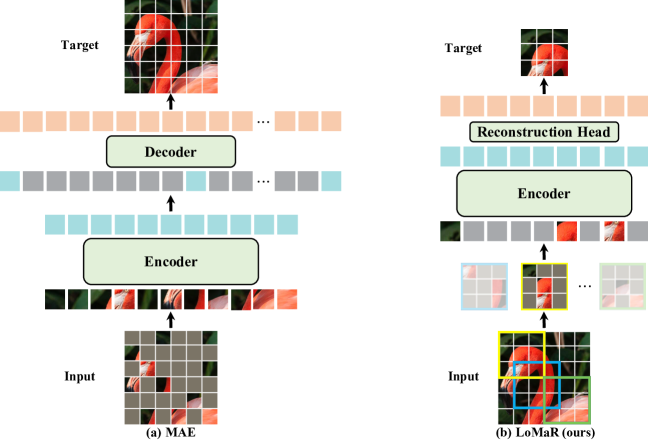
Figure 2: The illustration of our model. During the pretraining, it randomly samples several windows, and masks a random subset of patches from each window, e.g. 80%, for reconstruction. All the masked and visible patches from the sampled region are input into the encoder. Finally, we recover the missing patches with a simple reconstruction head (a MLP layer).

Self-supervised Learning For Images. The past few years have witnessed the boom of self-supervised learning. Existing techniques can be roughly categorized as discriminative [3, 42, 21] and generative. The prominent discriminative approach, instance discrimination, distinguishes different views of the same data instance from other instances [56, 41, 25, 10, 22, 13]. The most representative works include BYOL [22] , MOCO [12, 14, 25], and SimCLR [10, 11]. The generative approach includes autoregressive prediction [23, 9] and autoencoders, which we discuss next.

Autoencoders for Representation Learning. An autoencoder, which aims to learn a representation from which the original input can be reconstructed, has been a popular choice for representation learning since the dawn of deep learning [27, 5, 4]. The autoencoding problem is inherently ill-posed due to the existence of a trivial solution: a network entirely composed of identity mappings. Hence, it is necessary to apply some form of regularization, such as sparsity [48], input corruption [54], probability priors [31, 49], or adversarial discriminators [38].

In particular, denoising autoencoder [54], which attempts to recover the original input from a corrupted version, has received significant research attention. Variations include solving jigsaw puzzles [40], color restoration [61, 32], spatial relation recovery [17], inpainting [43], and so on. Recently, BEiT [2] proposes to encode image patches as a dictionary using dVAE [47] and predict the encoding of missing patches. PeCo [18] further improves BEiT with enforcing perceptual similarity from dVAE. MAE [24] reconstructs directly the missing pixels. CiM [20] replaces image patches with plausible alternatives and learns to recover the original and predict which patches are replaced.

3 Approach

LoMaR relies on a stack of Transformer [53] blocks to pretrain a large amount of unlabeled images by recovering the missing patches from corrupted images similar to MAE [24], but LoMaR differentiates from MAE in several key places. Fig. 2 compares the two side by side. In this section, we first revisit the MAE model and then describe the differences between LoMaR and MAE.

3.1 Background: Masked Autoencoder

The Masked Autoencoder (MAE) model [24], shown on the left side of Fig. 2, employs an asymmetric encoder-decoder architecture. The encoder takes in a subset of patches from an image and outputs latent representations for the patches. From those, the decoder reconstructs the missing patches. For an input image with resolution $h$ $\times$ $w$, MAE first divides it into a sequence of non-overlapping patches. Then, MAE randomly masks out a large proportion (e.g., 75%) of image patches. The positional encodings are added to each patch to indicate their spatial location. MAE first encodes the remaining patches into the latent representation space, and then feeds the latent representations together with placeholders for the masked patches into the decoder, which carries out the reconstruction. For each reconstructed image, MAE uses the mean squared error (MSE) with the original image in the pixel space as the loss function.

3.2 Local Masked Reconstruction (LoMaR)

We describe LoMaR by contrasting it with MAE from the following perspectives.

Local vs. Global Masked Reconstruction. MAE reconstructs each missing patch with patches sampled from the entire image. However, as indicated by Fig 1, usually only the patches in the proximity of the target patch contribute significantly to the reconstruction, suggesting that local information is sufficient for reconstruction. Therefore, we perform the masking and reconstruction on patches within a small region. Experiments find that a region size of 7$\times$7 patches leads to the best trade-off between accuracy and efficiency. On the other hand, similar to convolutional networks [26, 50], LoMaR has the translation invariance property due to the usage of small windows sampled in random spatial locations each iteration.

From the complexity perspective, the local masking and reconstruction are more computationally efficient than the global masking and reconstruction of MAE due to fewer tokens for operation. Suppose that each image can be divided into $h\times w$ patches. The time complexity for computing the self-attention is $\mathcal{O}(h^{2}w^{2})$. The complexity is quadratic to the number of patches and hard to scale up with large $hw$. However, for our local masked reconstruction, we sample $n$ windows where each contains $m\times m$ patches; Its computational complexity is $\mathcal{O}(hw+nm^{4})$, which has linear time complexity if we fix $m\times m$ as a constant window size. It can reduce the computational cost significantly if $nm^{4}\ll h^{2}w^{2}$.

Architecture. Instead of the asymmetric encoder-decoder of MAE, LoMaR applies a simple Transformer encoder architecture. We input all the visible and masked patches under a sampled region into the encoder. Although feeding the masked patches into the encoder can be deemed a less efficient operation than MAE that only inputs masked patches into the decoder, we find that inputting the masks in the early stages can enhance the visual representation and make it more robust to the smaller window sizes. It might be because the encoder can convert the masked patches back to their original RGB representation after multiple encoder layers’ interaction with the other visible patches. Those recovered masks in the hidden layers can implicitly contribute to the image representation. Therefore, we preserve the mask patches as the encoder input in LoMaR.

Relative positional encoding. LoMaR applies the relative positional encoding (RPE) instead of the absolute positional encoding in MAE. We apply the contextual RPE from [55], in which it introduces a learnable vector $r_{ij}$ for each query $i$ and key $j$ when computing the self-attention.

Implementation. Given an image, we first divide it into several non-overlapping patches. Each patch is linearly projected into an embedding. We randomly sample several square-shaped windows of $K\times K$ patches at different spatial locations. We then zero out a fixed percentage of patches within each window. After that, we feed all the patches, including visible and masked ones, from each window to the encoder in raster order. Following [55], the encoder applies learnable relative positional encoding in the self-attention layer. We convert the latent representations from the encoder output back to their original feature dimension with a simple MLP head, and then compute the mean squared error with the normalized ground-truth image.

4 Experiments

Methods	Pretraining Data	Epochs	Finetuning Resolution	Pretraining Time (h)	Top-1 Acc
No Pretraining	-	-	224$\times$224	-	82.3
DINO [7]	IN1K	300	224$\times$224	-	82.8
MoCov3 [14]	IN1K	600	224$\times$224	-	83.2
BEiT [2]	IN1K+DALLE [47]	800	224$\times$224	$\sim$285	83.2
MAE [24]	IN1K	400	224$\times$224	$\sim$58	83.1
MAE	IN1K	800	224$\times$224	$\sim$116	83.3
MAE	IN1K	1600	224$\times$224	$\sim$232	83.6
LoMaR (Ours)	IN1K	300	224$\times$224	$\sim$49	83.3
LoMaR (Ours)	IN1K	400	224$\times$224	$\sim$66	83.6
LoMaR (Ours)	IN1K	800	224$\times$224	$\sim$132	83.8
LoMaR (Ours)	IN1K	1600	224$\times$224	$\sim$264	84.1
$\text{LoMaR}_{8\times 8}$ (Ours)	IN1K	400	224$\times$224	$\sim$66	84.3
$\text{BEiT}_{\text{384}}$ [2]	IN1K+DALLE	800	384$\times$384	$\sim$285	84.6
$\text{MAE}_{\text{384}}$ [24]	IN1K	1600	384$\times$384	$\sim$232	$\text{84.8}^{*}$
$\text{LoMaR}_{\text{384}}$ (Ours)	IN1K	800	384$\times$384	$\sim$132	85.2
$\text{LoMaR}_{\text{384}}$ (Ours)	IN1K	1600	384$\times$384	$\sim$264	85.4

Table 1: Image classification results on the ImageNet-1K (IN1K) dataset [16]. All baselines excluding $\text{LoMaR}_{8\times 8}$ adopt the ViT B/16 model [19] and are pretrained on 224$\times$224 images. $\text{LoMaR}_{8\times 8}$ applies ViT B/8 as the backbone. * denotes our reproduced results based on the officially released code and pretrained models. The pretraining time are all computed on 4 NVIDIA A100 GPUs.

We examine the performance of LoMaR by pretraining and finetuning on ImageNet-1K [16] dataset with the following procedure. First, we perform the self-supervised pretraining on the ImageNet-1K training dataset without label information. Then, we finetune the pretrained model on ImageNet-1K with supervision from the labels. During finetuning, we feed all the image patches to the model and take the average of their features as the final representation for classification. We follow the same experimental settings as MAE [24]; detailed hyperparameters can be found in the supplementary material.

4.1 Comparison with Other Self-supervised Approaches

Table 1 summarizes the results of different self-supervised learning approaches. All models are pretrained self-supervisedly on ImageNet-1K [16] under the 224$\times$224 resolution and finetuned on labeled ImageNet-1K. LoMaR reaches the best result of MAE, 83.6%, after only 400 epochs of pretraining. When pretrained for 1,600 epochs, its performance further improves to 84.1%. When finetuned under the 384$\times$384 resolution, LoMaR reaches an accuracy of 85.4%, 0.6% higher than the best baseline. Overall, LoMaR outperforms strong baselines with less pretraining time.

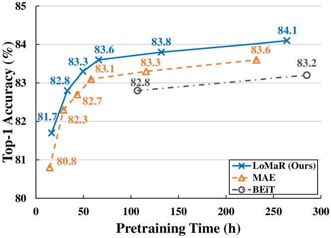
Figure 3: Computational efficiency evaluation: We compute their ImageNet-1K top-1 accuracy per pretraining time.

Efficiency analysis. The Fig. 3 and Table 1 show the comparison of the computational efficiency among LoMaR, MAE [24] and BEiT [2]. We carefully tuned all models to achieve the best load balancing between the GPU and the CPU and the maximal image throughput during training. We do this by adjusting ghost batch size [29] while keeping the total batch size constant for all models. We observe that, compared to baselines, LoMaR consistently achieves the same or higher accuracy in less pretraining time. Specifically, pretraining MAE with 1,600 epochs achieves 83.6% accuracy but takes about 232 hours. LoMaR reaches the same accuracy within $\sim$66 hours of pretraining, which is 3.5$\times$ faster. BEiT requires $285$ pretraining hours to get 83.2% accuracy. In contrast, LoMaR obtains a similar result within $\sim$49 hours, which translates to 5.8$\times$ time savings.

Pretraining on small patches. We also evaluate our model on smaller patches with 8$\times$8 pixels instead of the usual 16$\times$16 pixels. We employ ViT B/8 [19] as a backbone in Table 1. We pretrain LoMaR with 7$\times$7 windows (4 views per image) on 224$\times$224 images for 400 epochs. It is worth noting that this incurs the same amount of computation time (about 66 hours) as 16$\times$16 patches. The model accuracy after finetuning increases from 83.6% to 84.3% compared to 16$\times$16 patches. However, similar experiments are costly for MAE and BEiT, as smaller patches substantially increase the number of patches for operation and lead to the high cost of self-attention. In our experiments, the pretraining of MAE with their official code under 8$\times$8 patches crashes due to numerical issues.

Efficiency on high-resolution images. To evaluate the efficiency of self-supervised learning behaviors over higher-resolution images, we pretrain LoMaR, MAE, and BEiT over the image size of 384 and 448 on the ImageNet-1K dataset. We show their pretraining efficiency and accuracy in Fig. 4. For MAE, we follow their default settings during pretraining; Sample 75% patches as masks. For LoMaR, we set the number of views to 6 and 9 for resolutions of 384 and 448 to cover more visible patches per image. We pretrain all the models with 300 epochs and finetune them under the same image resolution. The results demonstrate that LoMaR consistently outperforms other models within substantially less pretraining time. , which scales linearly with the window numbers. In contrast, the pretraining time of MAE and BEiT scales quadratically as the resolution increases. As a result, LoMaR is 2.5$\times$ faster than MAE (accuracy +0.2%) and 5.0$\times$ faster than BEiT (accuracy +0.8%) on 384$\times$384 images, and for the resolution of 448$\times$448, it is 3.1$\times$ faster than MAE (accuracy +0.2%) and 5.3$\times$ faster than BEiT (accuracy +0.6%).

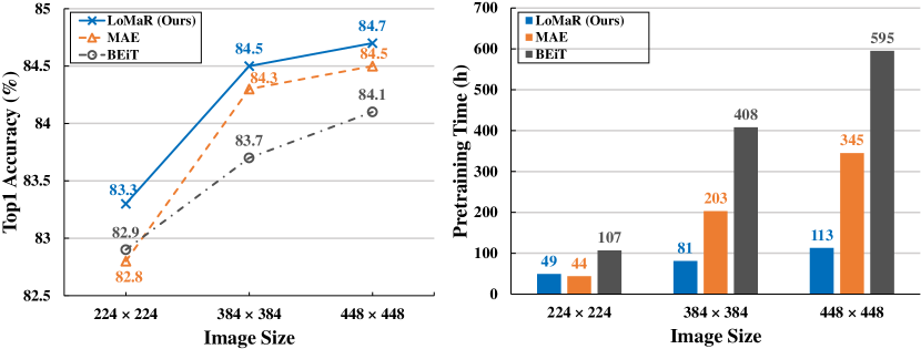
Figure 4: High-resolution image pretraining. All the models are pretrained for 300 epochs on 4 A100 GPUs. We report their pretraining time and top-1 accuracy on ImageNet-1K val dataset. For LoMaR, we sample 6 and 9 windows per image for the resolution of 384 and 448, respectively.

Object detection and instance segmentation. We finetune our model end-to-end on MS COCO [34] for the object detection and instance segmentation tasks. We replace the ViT backbone with our pretrained LoMaR model in the ViTDet [33] and ViTAE [60] frameworks. We report object detection results in $\text{AP}^{\text{box}}$ and instance segmentation results in $\text{AP}^{\text{mask}}$.

We provide the results in Table 2. It shows the consistent improvement of LoMaR on COCO object detection benchmark. Under ViTDet, LoMaR surpasses MAE by 0.3 $\text{AP}^{\text{box}}$ and 0.3 $\text{AP}^{\text{mask}}$. When applying the LoMaR pretrained for 1,600 epochs under the 384$\times$384 resolution, it further improves to 51.6 $\text{AP}^{\text{box}}$ and 45.9 $\text{AP}^{\text{mask}}$. In the ViTAE framework, LoMaR improves over MAE by 0.4 $\text{AP}^{\text{box}}$ and 0.4 $\text{AP}^{\text{mask}}$, respectively.

Backbone	ViTDet*[33]		ViTAE [60]
	$\text{AP}^{\text{box}}$	$\text{AP}^{\text{mask}}$	$\text{AP}^{\text{box}}$	$\text{AP}^{\text{mask}}$
MAE	$\text{51.1}^{*}$	$\text{45.4}^{*}$	51.6	45.8
LoMaR	51.4	45.7	51.8	46.0
$\text{LoMaR}_{\text{384}}$	51.6	45.9	52.0	46.2

Table 2: Object detection and instance segmentation results on MS COCO under two ViT frameworks. * denotes reproduced results with the code from [60]. $\text{LoMaR}_{\text{384}}$ denotes the model pretrained on 384$\times$384 images. Other models are pretrained on 224$\times$224 images.

4.2 Integration to BEiT

Our core idea, local masked reconstruction, can be easily integrated into other generative self-supervised learning methods. To examine its effectiveness in a different paradigm, we integrate it to BEiT [2]. Specifically, we randomly sample four 7$\times$7 windows and feed them into the BEiT model, and pretrain for 300 epochs, while retaining all other experimental settings as the original BEiT. Results in Table 3 show that this strategy improves the accuracy from 82.8% to 83.4%, which is higher than the original BEiT pretrained for 800 epochs.

Method	Epochs	Pretraining Time (h)	Top-1 Acc
BEiT [2]	300	$\sim$107	82.8
BEiT	800	$\sim$285	83.2
BEiT + Our approach	300	$\sim$102	83.4

Table 3: The results of applying our method on BEiT approach

4.3 Ablative Experiments

We conducted many ablation experiments to explore properties such as the window size, masking ratio, and architecture design, and share our findings in this section. We performed all the ablation experiments under 4 NVIDIA A100 GPUs with the same setting for fair comparisons.

Window Size	5$\times$5	7$\times$7	9$\times$9	11$\times$11	14$\times$14
Views	8	4	3	2	1

Table 4: The ratio between window size and number of views per image, as utilized by LoMaR.

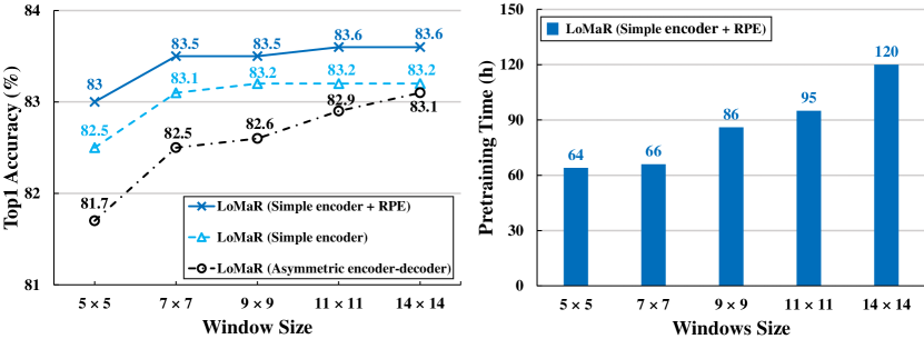
Figure 5: Left: accuracy of LoMaR under different architectures and window sizes. Right: pretraining time in hours vs. different window size for LoMaR with relative positional encoding (RPE).

Architecture. Fig. 5 compares different architectures, including a simple encoder (with both visible and masked patches as input) and an asymmetric encoder-decoder architecture, as employed by MAE. Initially, we sample 75% patches as the masks following the guidance of MAE. We use the absolute positional encoding (APE) for both architectures by default. We ablate these two architectures with different masked reconstruction windows, and it shows that a simple encoder can always outperform the asymmetric encoder-decoder. Moreover, the performance gap is further magnified when we decrease the window size from 14 to 7, suggesting that a simple encoder is more robust to smaller window sizes than MAE-like architecture.

We also compare the version of LoMaR with relative positional encoding (Simple encoder + RPE) and absolute positional encoding (Simple encoder). The results show an average improvement of 0.3 acc across different window sizes, demonstrating the benefit of RPE.

Window size. We create versions LoMaR (Simple encoder + RPE) with multiple different window sizes such as 5$\times$5, 7$\times$7, 9$\times$9, 11$\times$11 and 14$\times$14. One caveat is that the smaller window covers much fewer visible patches than the larger ones, which creates unfair comparisons. To encourage fairness, we assign different numbers of views for each window size, shown in Table 4, so that all conditions have similar number of visible patches in training.

The results in Fig 5 indicate that MAE performance remains stable while we decrease the window size from 14 to 7, but exhibits a sharp when the window size is reduced to 5. On the other hand, a larger window size usually results in higher computational cost, as shown in Fig 5 (right); the 14$\times$14 window incurs almost twice the pretraining time of the 7$\times$7 window. Therefore, from both the efficiency and accuracy perspective, window size 7$\times$7 can be deemed an optimal trade-off for local masked reconstruction.

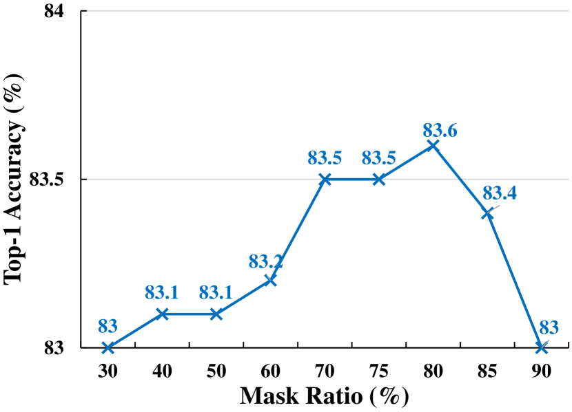
Figure 6: Mask ratio ablations: We pretrain LoMaR with different mask ratios for 400 epochs

Mask ratio. We also explore the best mask ratio under the local masked reconstruction scenario (see Fig. 6). We train our previous best setting (Simple encoder + window size 7$\times$7 + RPE) on different mask ratios, ranging from 30% to 90%. The results show that too low (30%) or too high (90%) mask ratio are not optimal since they over-simplify or complicate the training task. We found that the 80% mask ratio can result in the best performance, differentiating from the 60% mask ratio observed in MAE for best finetuning performance. With this motivation, we employ the 80% mask ratio in our experiments.

4.4 Visualization of Reconstructed Images

We qualitatively show the reconstruction performance of our pretrained model in Fig. 7. We randomly sample several images from ImageNet-1K [16] and MS COCO[34]. After that, we sample a region containing 7$\times$7 patches in every image and zero out 80% patches in the window for reconstruction. It can be seen that LoMaR is capable of generating plausible images, which also confirms our initial conjecture that the missing patches can be recovered from the local surrounding patches alone.

We show the reconstruction performance under different masking ratios in Fig. 8. For each image, we sample a window and randomly mask 60%, 70%, 80%, and 90% patches for reconstruction. We found that LoMaR can plausibly recover the corrupted image in various masking scales; It can still successfully reconstruct the images even with only 5 visible patches as the clues (90% masking). This indicates that LoMaR has learned high-capacity models and can infer complex reconstructions.

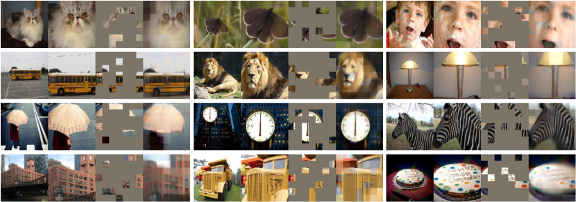
Figure 7: Example results on ImageNet (upper two rows) and COCO (lower two rows) validation images. We mask 80% patches out and reconstruct them with our pretrained model. For each image reconstruction figure, we split them into 4 parts: 1) the left-most is the original image. 2) the second-left is the sampled window (7$\times$7 patches). 3) The second-right is the masked image. 4) The right-most is our reconstructed image.

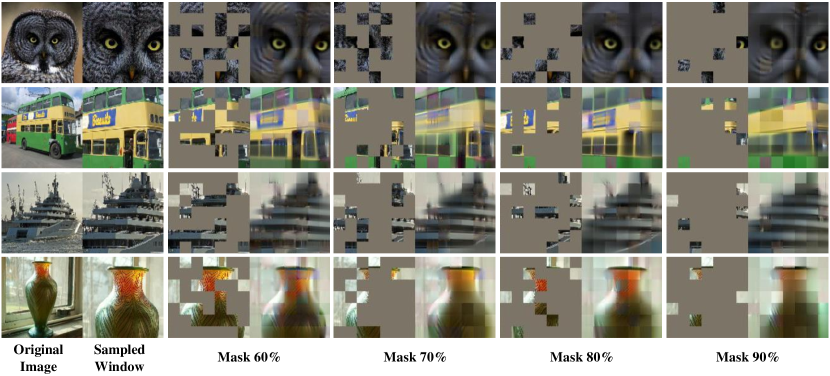
Figure 8: Reconstruction examples of sampled ImageNet (upper two rows) and COCO (lower two rows) validation images under different masking ratios ranging from 60% to 90%.

5 Discussion and Limitations

Self-supervised learning (SSL) can benefit from training with massive amount of unlabeled data, which has brought many promising results [30, 45, 46, 6, 24, 2, 14, 8]. However, their high computational demands remain a significant concern under large-scale pretraining. In our study, we observe that the local masked reconstruction (LoMaR) for generative SSL is more efficient than the global version used by the influential works of MAE [24] and BEiT [2]. LoMaR demonstrates good generalization in image classification, instance segmentation and object detection; it can be easily incorporated into both MAE and BEiT. LoMaR holds the promise to scale up SSL to even bigger datasets and higher resolution [44, 52] as well as more computation-intensive datasets such as videos [39].

Another advantage of LoMaR lies in efficiency gain when the number of image patches increases, such as for the high-resolution images or small patches of 8$\times$8. The primary reason is that LoMaR restricts the self-attention within a local window, and its computational complexity grows linearly with the number of sampled windows per image. This characteristic enables efficient pretraining under high image resolution, which would be prohibitively expensive for other SSL methods. It can benefit many vision tasks such as object detection or instance segmentation, which require dense prediction at the pixel level.

Despite the high pretraininig efficiency gain of LoMaR over other baselines for high-resolution images, LoMaR’s efficiency improvement over lower-resolution images is somewhat limited compared to MAE [24]. While training the same number of epochs on 224$\times$224 images, LoMaR is 2.2$\times$ faster than BEiT [2] which also has masked patches as the encoder input, but it consumes around 10% extra pretraining time than MAE. This phenomenon is mainly due to two reasons: 1) The MAE encoder takes as input only the visible patches, but the LoMaR encoder takes the masked patches in addition, which results in a similar number of patches under low resolution. 2) LoMaR also adopts a contextual-aware relative positional encoding [55], which introduces additional computation. However, its efficiency can be further improved by either under-sampling the windows or moving the masked patches into the later encoder layers. We hope the local masked reconstruction idea can be adapted into a more efficient model architecture in future work.

6 Supplementary

6.1 ImageNet Experiments

We follow the MAE [24] settings to launch our experiments. The major implementation difference is the model implementation and positional encoding. We apply a 12-layer ViT [19] as a backbone. On top of the ViT, LoMaR adds an MLP layer for the linear projection. We also employ the relative positional encoding [55] in our LoMaR to model the relative positional relation among the patches within the sampled local window.

Pretraining. We apply the batch size 4096 by default during the pretraining. We do not perform any data augmentation strategies. The base learning rate is 1.5e-4. We use AdamW [37] to optimize the model parameters with weight decay 0.05. The cosine decay [36] is applied to schedule the learning rate changes. We only apply the RandomResizedCrop augmentation strategy. The warm-up epoch is 40 for pretraining 1,600 epochs, 20 for pretraining 800 epochs, and 10 for pretraining 400 epochs.

Finetuning. During the finetuning stage, we directly use the pretrained visual encoder and add another classification head. The base learning rate is 1e-3. We apply the adamW [37] optimizer and cosine decay [36] learning rate scheduler in our implementation. We finetune the models for 100 epochs, same as MAE. The batch size is 1024. The warm-up epoch is 5. The mixup [59] rate is 0.8. We also aggregate the features from all the image patches to generate the whole image representation through average pooling.

6.2 COCO Object Detection Experiments

We follow ViTDet [33] and ViTAE [60] experimental settings and replace the original MAE model with our pretrained LoMaR. We also integrate our relative positional encoding into their model. For the image resolution of 224$\times$224, we apply our pretrained LoMaR (4 sampled windows per image + 1,600 pretraining epochs). For the image resolution of 384$\times$384, we apply our pretrained LoMaR (9 sampled windows per image + 1,600 pretraining epochs). The image patch size is 16$\times$16. We train 25 epochs with the batch size of 64. The input image size is 1024$\times$1024.

7 More reconstruction results

We sample more images from ImageNet [16] and MS COCO [34] and perform our local masked reconstruction. The visualization results are shown in the Fig. 9 and 10.

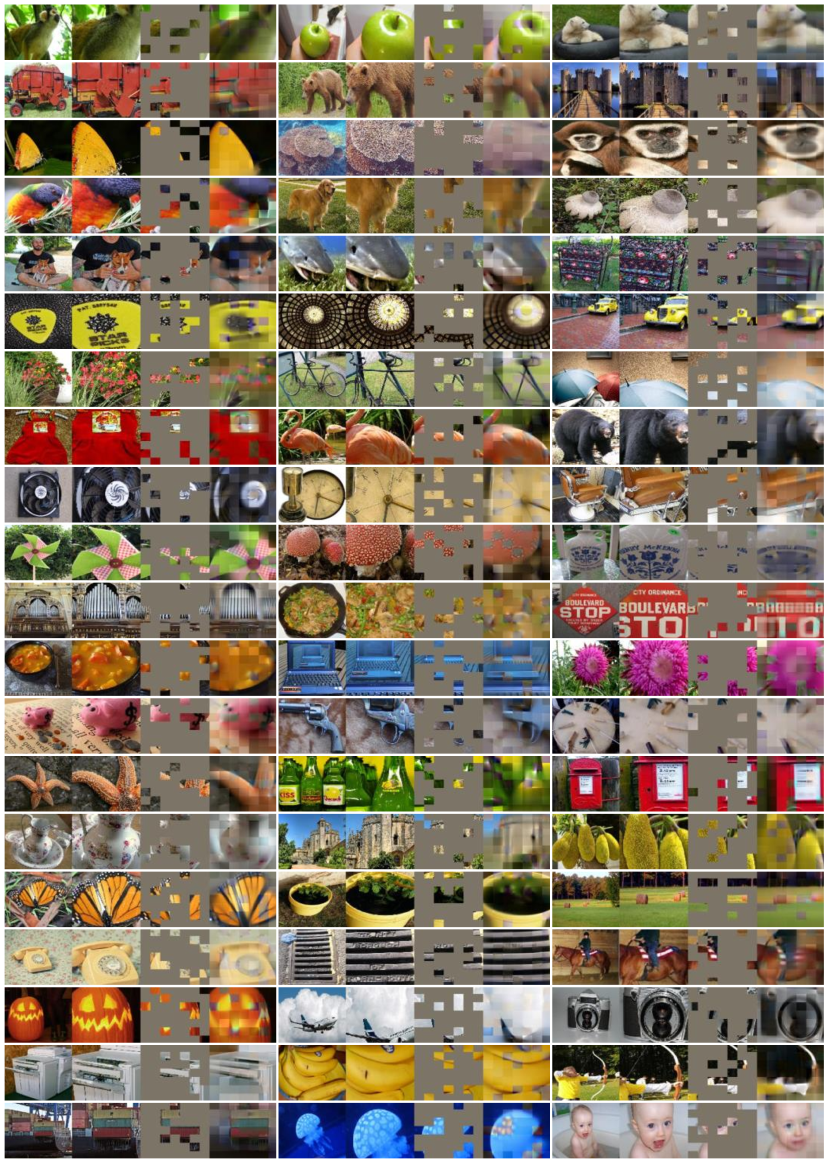
Figure 9: More reconstruction examples of our pretrained model on ImageNet validation images. The masking ratio is 80%. For each image reconstruction figure, we split them into 4 parts: 1) the left-most is the original image. 2) the second-left is the sampled window (7×7 patches). 3) The second-right is the masked image. 4) The right-most is our reconstructed image

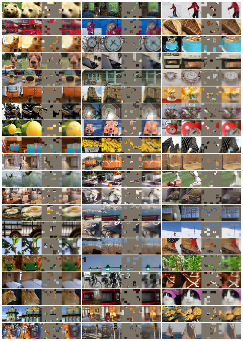
Figure 10: More reconstruction examples of our pretrained model on COCO validation images. The masking ratio is 80%. For each image reconstruction figure, we split them into 4 parts: 1) the left-most is the original image. 2) the second-left is the sampled window (7×7 patches). 3) The second-right is the masked image. 4) The right-most is our reconstructed image

References

- [1] P. Bachman, R. D. Hjelm, and W. Buchwalter. Learning representations by maximizing mutual information across views. Advances in neural information processing systems, 32, 2019.
- [2] H. Bao, L. Dong, S. Piao, and F. Wei. BEit: BERT pre-training of image transformers. In International Conference on Learning Representations, 2022.
- [3] S. Becker and G. E. Hinton. Self-organizing neural network that discovers surfaces in random-dot stereograms. Nature, 355(6356):161–163, 1992.
- [4] Y. Bengio, A. Courville, and P. Vincent. Representation learning: A review and new perspectives. IEEE transactions on pattern analysis and machine intelligence, 35(8):1798–1828, 2013.
- [5] Y. Bengio, P. Lamblin, D. Popovici, and H. Larochelle. Greedy layer-wise training of deep networks. In Proceedings of the 19th International Conference on Neural Information Processing Systems, NeurIPS’06, page 153–160, Cambridge, MA, USA, 2006. MIT Press.
- [6] T. Brown, B. Mann, N. Ryder, M. Subbiah, J. D. Kaplan, P. Dhariwal, A. Neelakantan, P. Shyam, G. Sastry, A. Askell, et al. Language models are few-shot learners. Advances in neural information processing systems, 33:1877–1901, 2020.
- [7] M. Caron, H. Touvron, I. Misra, H. Jégou, J. Mairal, P. Bojanowski, and A. Joulin. Emerging properties in self-supervised vision transformers. In Proceedings of the IEEE/CVF International Conference on Computer Vision, pages 9650–9660, 2021.
- [8] J. Chen, H. Guo, K. Yi, B. Li, and M. Elhoseiny. Visualgpt: Data-efficient adaptation of pretrained language models for image captioning. arXiv preprint arXiv:2102.10407, 2021.
- [9] M. Chen, A. Radford, R. Child, J. Wu, H. Jun, D. Luan, and I. Sutskever. Generative pretraining from pixels. In International Conference on Machine Learning, pages 1691–1703. PMLR, 2020.
- [10] T. Chen, S. Kornblith, M. Norouzi, and G. Hinton. A simple framework for contrastive learning of visual representations. In International conference on machine learning, pages 1597–1607. PMLR, 2020.
- [11] T. Chen, S. Kornblith, K. Swersky, M. Norouzi, and G. E. Hinton. Big self-supervised models are strong semi-supervised learners. Advances in neural information processing systems, 33:22243–22255, 2020.
- [12] X. Chen, H. Fan, R. Girshick, and K. He. Improved baselines with momentum contrastive learning. arXiv preprint arXiv:2003.04297, 2020.
- [13] X. Chen and K. He. Exploring simple siamese representation learning. In Proceedings of the IEEE/CVF Conference on Computer Vision and Pattern Recognition, pages 15750–15758, 2021.
- [14] X. Chen, S. Xie, and K. He. An empirical study of training self-supervised vision transformers. In Proceedings of the IEEE/CVF International Conference on Computer Vision, pages 9640–9649, 2021.
- [15] R. Child, S. Gray, A. Radford, and I. Sutskever. Generating long sequences with sparse transformers. URL https://openai.com/blog/sparse-transformers, 2019.
- [16] J. Deng, W. Dong, R. Socher, L.-J. Li, K. Li, and L. Fei-Fei. Imagenet: A large-scale hierarchical image database. In 2009 IEEE Conference on Computer Vision and Pattern Recognition.
- [17] C. Doersch, A. Gupta, and A. A. Efros. Unsupervised visual representation learning by context prediction. In Proceedings of the IEEE international conference on computer vision, pages 1422–1430, 2015.
- [18] X. Dong, J. Bao, T. Zhang, D. Chen, W. Zhang, L. Yuan, D. Chen, F. Wen, and N. Yu. Peco: Perceptual codebook for bert pre-training of vision transformers. arXiv preprint arXiv:2111.12710, 2021.
- [19] A. Dosovitskiy, L. Beyer, A. Kolesnikov, D. Weissenborn, X. Zhai, T. Unterthiner, M. Dehghani, M. Minderer, G. Heigold, S. Gelly, et al. An image is worth 16x16 words: Transformers for image recognition at scale. arXiv preprint arXiv:2010.11929, 2020.
- [20] Y. Fang, L. Dong, H. Bao, X. Wang, and F. Wei. Corrupted image modeling for self-supervised visual pre-training. arXiv preprint arXiv:2202.03382, 2022.
- [21] S. Gidaris, P. Singh, and N. Komodakis. Unsupervised representation learning by predicting image rotations. In International Conference on Learning Representations, 2018.
- [22] J.-B. Grill, F. Strub, F. Altché, C. Tallec, P. Richemond, E. Buchatskaya, C. Doersch, B. Avila Pires, Z. Guo, M. Gheshlaghi Azar, et al. Bootstrap your own latent-a new approach to self-supervised learning. Advances in Neural Information Processing Systems, 33:21271–21284, 2020.
- [23] T. Han, W. Xie, and A. Zisserman. Video representation learning by dense predictive coding. In Proceedings of the IEEE/CVF International Conference on Computer Vision Workshops, pages 0–0, 2019.
- [24] K. He, X. Chen, S. Xie, Y. Li, P. Dollár, and R. Girshick. Masked autoencoders are scalable vision learners. arXiv preprint arXiv:2111.06377, 2021.
- [25] K. He, H. Fan, Y. Wu, S. Xie, and R. Girshick. Momentum contrast for unsupervised visual representation learning. In Proceedings of the IEEE/CVF conference on computer vision and pattern recognition, pages 9729–9738, 2020.
- [26] K. He, X. Zhang, S. Ren, and J. Sun. Deep residual learning for image recognition. In Proceedings of the IEEE conference on computer vision and pattern recognition, pages 770–778, 2016.
- [27] G. E. Hinton and R. R. Salakhutdinov. Reducing the dimensionality of data with neural networks. Science, 313(5786):504–507, 2006.
- [28] R. D. Hjelm, A. Fedorov, S. Lavoie-Marchildon, K. Grewal, P. Bachman, A. Trischler, and Y. Bengio. Learning deep representations by mutual information estimation and maximization. In International Conference on Learning Representations, 2018.
- [29] E. Hoffer, I. Hubara, and D. Soudry. Train longer, generalize better: Closing the generalization gap in large batch training of neural networks. In Proceedings of the 31st International Conference on Neural Information Processing Systems, NIPS’17, page 1729–1739, Red Hook, NY, USA, 2017. Curran Associates Inc.
- [30] J. D. M.-W. C. Kenton and L. K. Toutanova. Bert: Pre-training of deep bidirectional transformers for language understanding. In Proceedings of NAACL-HLT, pages 4171–4186, 2019.
- [31] D. P. Kingma and M. Welling. Auto-encoding variational bayes. arXiv preprint arXiv:1312.6114, 2013.
- [32] G. Larsson, M. Maire, and G. Shakhnarovich. Learning representations for automatic colorization. In European conference on computer vision, pages 577–593. Springer, 2016.
- [33] Y. Li, H. Mao, R. Girshick, and K. He. Exploring plain vision transformer backbones for object detection. arXiv preprint arXiv:2203.16527, 2022.
- [34] T.-Y. Lin, M. Maire, S. Belongie, J. Hays, P. Perona, D. Ramanan, P. Dollár, and C. L. Zitnick. Microsoft coco: Common objects in context. In European conference on computer vision, pages 740–755. Springer, 2014.
- [35] Z. Liu, Y. Lin, Y. Cao, H. Hu, Y. Wei, Z. Zhang, S. Lin, and B. Guo. Swin transformer: Hierarchical vision transformer using shifted windows. In Proceedings of the IEEE/CVF International Conference on Computer Vision, pages 10012–10022, 2021.
- [36] I. Loshchilov and F. Hutter. Sgdr: Stochastic gradient descent with warm restarts. 2016.
- [37] I. Loshchilov and F. Hutter. Decoupled weight decay regularization. In International Conference on Learning Representations, 2018.
- [38] A. Makhzani, J. Shlens, N. Jaitly, I. Goodfellow, and B. Frey. Adversarial autoencoders. arXiv preprint arXiv:1511.05644, 2015.
- [39] A. Miech, D. Zhukov, J.-B. Alayrac, M. Tapaswi, I. Laptev, and J. Sivic. Howto100m: Learning a text-video embedding by watching hundred million narrated video clips. In Proceedings of the IEEE/CVF International Conference on Computer Vision, pages 2630–2640, 2019.
- [40] M. Noroozi and P. Favaro. Unsupervised learning of visual representations by solving jigsaw puzzles. In European conference on computer vision, pages 69–84. Springer, 2016.
- [41] A. v. d. Oord, Y. Li, and O. Vinyals. Representation learning with contrastive predictive coding. arXiv preprint arXiv:1807.03748, 2018.
- [42] D. Pathak, R. Girshick, P. Dollár, T. Darrell, and B. Hariharan. Learning features by watching objects move. In Proceedings of the IEEE conference on computer vision and pattern recognition, pages 2701–2710, 2017.
- [43] D. Pathak, P. Krahenbuhl, J. Donahue, T. Darrell, and A. A. Efros. Context encoders: Feature learning by inpainting. In Proceedings of the IEEE conference on computer vision and pattern recognition, pages 2536–2544, 2016.
- [44] A. Radford, J. W. Kim, C. Hallacy, A. Ramesh, G. Goh, S. Agarwal, G. Sastry, A. Askell, P. Mishkin, J. Clark, et al. Learning transferable visual models from natural language supervision. In International Conference on Machine Learning, pages 8748–8763. PMLR, 2021.
- [45] A. Radford, K. Narasimhan, T. Salimans, and I. Sutskever. Improving language understanding by generative pre-training. 2018.
- [46] A. Radford, J. Wu, R. Child, D. Luan, D. Amodei, I. Sutskever, et al. Language models are unsupervised multitask learners. OpenAI blog, 1(8):9, 2019.
- [47] A. Ramesh, M. Pavlov, G. Goh, S. Gray, C. Voss, A. Radford, M. Chen, and I. Sutskever. Zero-shot text-to-image generation. In International Conference on Machine Learning, pages 8821–8831. PMLR, 2021.
- [48] M. Ranzato, C. Poultney, S. Chopra, and Y. LeCun. Efficient learning of sparse representations with an energy-based model. In Advances in Neural Information Processing Systems, volume 19, 2006.
- [49] D. J. Rezende, S. Mohamed, and D. Wierstra. Stochastic backpropagation and approximate inference in deep generative models. In E. P. Xing and T. Jebara, editors, Proceedings of the 31st International Conference on Machine Learning, volume 32 of Proceedings of Machine Learning Research, pages 1278–1286, Bejing, China, 22–24 Jun 2014. PMLR.
- [50] K. Simonyan and A. Zisserman. Very deep convolutional networks for large-scale image recognition. arXiv preprint arXiv:1409.1556, 2014.
- [51] S. Sukhbaatar, É. Grave, P. Bojanowski, and A. Joulin. Adaptive attention span in transformers. In Proceedings of the 57th Annual Meeting of the Association for Computational Linguistics, pages 331–335, 2019.
- [52] C. Sun, A. Shrivastava, S. Singh, and A. Gupta. Revisiting unreasonable effectiveness of data in deep learning era. In Proceedings of the IEEE international conference on computer vision, pages 843–852, 2017.
- [53] A. Vaswani, N. Shazeer, N. Parmar, J. Uszkoreit, L. Jones, A. N. Gomez, Ł. Kaiser, and I. Polosukhin. Attention is all you need. Advances in neural information processing systems, 30, 2017.
- [54] P. Vincent, H. Larochelle, Y. Bengio, and P.-A. Manzagol. Extracting and composing robust features with denoising autoencoders. In Proceedings of the 25th International Conference on Machine Learning, ICML ’08, page 1096–1103, New York, NY, USA, 2008. Association for Computing Machinery.
- [55] K. Wu, H. Peng, M. Chen, J. Fu, and H. Chao. Rethinking and improving relative position encoding for vision transformer. In Proceedings of the IEEE/CVF International Conference on Computer Vision, pages 10033–10041, 2021.
- [56] Z. Wu, Y. Xiong, S. X. Yu, and D. Lin. Unsupervised feature learning via non-parametric instance discrimination. In Proceedings of the IEEE conference on computer vision and pattern recognition, pages 3733–3742, 2018.
- [57] J. Yang, C. Li, P. Zhang, X. Dai, B. Xiao, L. Yuan, and J. Gao. Focal self-attention for local-global interactions in vision transformers. arXiv preprint arXiv:2107.00641, 2021.
- [58] M. Zaheer, G. Guruganesh, K. A. Dubey, J. Ainslie, C. Alberti, S. Ontanon, P. Pham, A. Ravula, Q. Wang, L. Yang, et al. Big bird: Transformers for longer sequences. Advances in Neural Information Processing Systems, 33:17283–17297, 2020.
- [59] H. Zhang, M. Cisse, Y. N. Dauphin, and D. Lopez-Paz. mixup: Beyond empirical risk minimization. In International Conference on Learning Representations, 2018.
- [60] Q. Zhang, Y. Xu, J. Zhang, and D. Tao. Vitaev2: Vision transformer advanced by exploring inductive bias for image recognition and beyond. arXiv preprint arXiv:2202.10108, 2022.
- [61] R. Zhang, P. Isola, and A. A. Efros. Colorful image colorization. In European conference on computer vision, pages 649–666. Springer, 2016.