Formal Interpretability with Merlin-Arthur Classifiers

Abstract

We propose a new type of multi-agent interactive classifier that provides provable interpretability guarantees even for complex agents such as neural networks. These guarantees consist of bounds on the mutual information of the features selected by this classifier. Our results are inspired by the Merlin-Arthur protocol from Interactive Proof Systems and express these bounds in terms of measurable metrics such as soundness and completeness. Compared to existing interactive setups we do not rely on optimal agents or on the assumption that features are distributed independently. Instead, we use the relative strength of the agents as well as the new concept of Asymmetric Feature Correlation which captures the precise kind of correlations that make interpretability guarantees difficult. We test our results through numerical experiments on two small-scale datasets where high mutual information can be verified explicitly.

1 Introduction

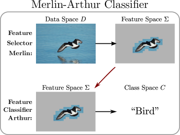
Figure 1: The Merlin-Arthur classifier consists of two interactive agents that communicate over an exchanged feature. This feature serves as an interpretation of the classification.

Safe deployment of Neural Network (NN) based AI systems in high-stakes applications requires that their reasoning be subject to human scrutiny. The field of Explainable AI (XAI) has thus put forth a number of interpretability approaches, among them saliency maps (Mohseni et al., 2021), mechanistic interpretability (Olah et al., 2018) and self-explaining networks (Alvarez Melis & Jaakkola, 2018). These have had some successes, such as detecting biases in established datasets (Lapuschkin et al., 2019). However, these approaches are motivated primarily by heuristics and come without any theoretical guarantees. Thus, their success cannot be verified. It has also been demonstrated for numerous XAI-methods that they can be manipulated by a clever design of the NNs (Slack et al., 2021, 2020; Anders et al., 2020; Dimanov et al., 2020). On the other hand, formal approaches to interpretability run into complexity barriers when applied to NNs and require an exponential amount of time to guarantee useful properties (Macdonald et al., 2020; Ignatiev et al., 2019). This makes any “right to explanation,” as codified in the EU’s GDPR (Goodman & Flaxman, 2017), unenforceable.

In this work, we design a classifier that guarantees feature-based interpretability under reasonable assumptions. For this, we connect classification to the Merlin-Arthur protocol (Arora & Barak, 2009) from Interactive Proof Systems (IPS), see Figure 1. Our setup consists of a classifer called Arthur (verifier) and 2 feature selectors referred to Merlin and Morgana (provers). Merlin and Morgana choose features from the input image and send them to Arthur. Merlin aims to send features that cause Arthur to correctly classify the underlying data point. Morgana instead selects features to convince Arthur of the wrong class. Arthur does not know who sent the feature and is allowed to say “Don’t know!” if he cannot discern the class. In this context, we can then translate the concepts of completeness and soundness from IPS to our setting. Completeness describes the probability that Arthur classifies correctly based on features from Merlin. Soundness is the probability that Arthur does not get fooled by Morgana, thus either giving the correct class or answering “Don’t know!”. These two quantities can be measured on a test dataset and are used to lower bound the information contained in features selected by Merlin.

1.1 Related Work

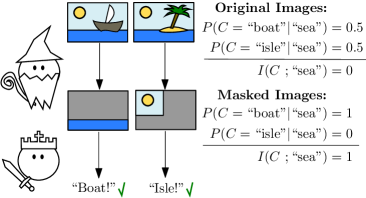
Figure 2: Illustration of “cheating” behaviour. In the original dataset, the features “sea” and “sky” appear equally in both classes “boat” and “island”. In the new set of images that Merlin creates by masking features of the original image, the “sea” feature is visible only in the images labelled “boat” and the “sky” feature is visible only in the images labelled “island”. Thus, these features now strongly indicate the class of the image. This allows Merlin to communicate the correct class with uninformative features — in contrast to our concept of an interpretable classifier.

Formal approaches to interpretability, such as mutual information (Chen et al., 2018) or Shapley values Frye et al. (2020), generally make use of partial inputs to the classifier. These partial inputs are realised by considering distributions over inputs conditioned on the given information. However, modelling these distributions is difficult for non-synthetic data. This has been pursued practically by training a generative model as in Chattopadhyay et al. (2022). But as of yet there is no approach that provides a bound on the quality of these models. We discuss these approaches and their challenges in greater detail in Section A.2.

Interactive classification in form of a prover-verifier setting has emerged as a way to design inherently interpretable classifiers (Lei et al., 2016; Bastings et al., 2019). In this setup, the feature selector chooses a feature from a data point and presents it to the classifier who decides the class, see Figure 2. The classification accuracy is meant to guarantee the informativeness of the exchanged features. However, it was noted by Yu et al. that the selector and the classifier can cooperate to achieve high accuracy while communicating over uninformative features, see Figure 2 for an illustration of this “cheating”. Thus, one cannot hope to bound the information content of features via accuracy alone. Chang et al. include an adversarial selector to prevent the cheating. The reasoning is that any “cheating” strategy can be exploited by the adversary to fool the classifier into stating the wrong class, see Figure 3 for an illustration. Anil et al. investigate scenarios in which the three-player setup converges to an equilibrium of perfect completeness and soundness. However, this work assumes that a perfect strategy exists and can be reached through training. For many classification problems, such as the ones we explore in our experimental section, no strategies are perfectly sound and complete when the size of the certificate is limited.

Alternative adversarial setups have been proposed in Yu et al. (2019) and Irving et al. (2018), but no information bounds were formulated for them. We discuss these ideas and their challenges in detail in Section A.4.

An additional theoretical focus has been the learnability of interpretations Goldwasser et al. (2021); Yadav et al. (2022). In this work, we do not focus on the question of learnability. We instead propose to evaluate soundness and completeness directly on the test dataset, as state-of-the-art models are to complex to guarantee generalisation from a realistic number of training samples.

The closest work is the framework proposed by Chang et al.. The setup is basically the same, except that for choices that matter only for numerical implementation, see Section A.3 for an in-depth discussion. The authors show that the best strategy for the provers is to select features with high mutual information wrt to the class. However, these results have three restriction that we resolve in this work: (i) The features are assumed to be independently distributed. This is an unrealistic assumption for most datasets where features are generally correlated. In this regime simply modelling the data distribution directly is possible. (ii) The provers can only select one feature at a time without context. This strategy is unlikely to yield useful rationalisations for most types of data where the importance of a feature strongly depends on the features surrounding it, like images and text. The authors do not impose this restriction for their numerical investigation. (iii) The result is non-quantitative. Since we cannot expect the agents to play optimally on complicated data we need measures on how well they play and how that relates to the mutual information of the features.

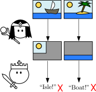
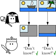
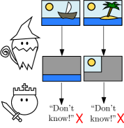
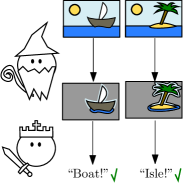
a)	b)	c)	d)

Figure 3: Strategy evolution with Morgana. a) Due to the “cheating” strategy from Figure 2, Arthur expects the “sea” feature for boats and the “sky” for islands. Morgana can exploit this and send the “sky” feature to trick Arthur into classifying a “boat” image as an “island” (and vice versa with “sea”). b) To not be fooled into the wrong class when represented with an ambiguous feature, Arthur refrains from giving a concrete classification. c) Since Arthur does not know who sends the features, he now cannot leverage the uninformative features sent by Merlin. d) Merlin adapts his strategy to only send unambiguous features that cannot be used by Morgana to fool Arthur.

1.2 Contribution

We provide, what we believe, the first quantitative lower bound on the information content of the features in an interpretive setup without the need to trust a model of the data distribution. Additionally, we improve existing analyses in the following ways:

1. We do not assume our agents to be optimal. In 2.8 Merlin is allowed to have an arbitrary strategy and in 2.12 all three players can play suboptimally. We rather rely on the relative strength of Merlin and Morgana for our bound. We also allow our provers to select the features with the context of the full datapoint.

2. We do not make the assumption that features are independently distributed. Instead, we introduce the notion of Asymmetric Feature Correlation (AFC) that captures which correlations make an information bound difficult. In 2.8 we circumvent the issue by reducing the dataset, and in 2.12 we incorporate the AFC explicitly. In Section 4 we discuss why the AFC also matters for other interactive settings.

2 Theoretical Framework

In this section we develop the theoretical framework for the Merlin-Arthur classifier. A key aspect is the notion of a feature. What reasonably constitutes a feature strongly depends on the context and prior work often considered subsets of the input as features. W.l.o.g we will stay with this convention for ease of notation. But nothing in our framework relies on these specifics and our theoretical results can be extended to more abstract queries Chen et al. (2018); Ribeiro et al. (2018).

Given a vector $\mathbf{x}$ of dimension $d$, we use $\mathbf{x}_{S}$ to represent a vector made of the components of $\mathbf{x}$ indexed by the set $S\subseteq\{1,\dots,d\}$.

Definition 2.1.

Given a dataset $D\subset[0,1]^{d}$, we define the corresponding partial dataset $D_{p}$ as

$$D_{p}=\bigcup_{\mathbf{x}\in D}\bigcup_{S\subset[d]}\mathbf{x}_{S}.$$

The set $D$ is possibly infinite, e.g. the set of all images of hand-written digits. $\mathcal{D}$ is a distribution on this set. The finite training and test sets, e.g. MNIST, for our algorithms are assumed to be faithful samples from this distribution.

Every vector $\mathbf{x}\in D\subset[0,1]^{d}$ can be uniquely represented as a set $\mathopen{}\left\{(1,x_{1}),(2,x_{2}),\dots,(d,x_{d})\right\}\mathclose{}$. A partial vector $\mathbf{z}\in D_{p}$ can then be a subset of $\mathbf{x}$. Thus, $\mathbf{z}\subseteq\mathbf{x}$ indicates that $\mathbf{x}$ contains the feature $\mathbf{z}$. The set $D_{p}$ might be further restricted to include only connected sets (for image or text data) or only sets of a certain size as in our numerical investigation.

We now define a data space. In our theoretical investigation we restrict ourselves to two classes and assume the existence of unique class for every data point. These are restrictions that we hope to relax in further research.

Definition 2.2 (Two-class Data Space).

We consider the tuple $\mathfrak{D}=(D,\mathcal{D},c)$ a two-class data space consisting of the dataset $D\subseteq[0,1]^{d}$, a probability distribution $\mathcal{D}$ along with the ground truth class map $c:D\rightarrow\mathopen{}\left\{-1,1\right\}\mathclose{}$. The class imbalance $B$ of a two-class data space is $\max_{l\in\mathopen{}\left\{-1,1\right\}\mathclose{}}{{\mathbb{P}_{\mathbf{x}\sim\mathcal{D}}\mathopen{}\left[c(\mathbf{x})=l\right]\mathclose{}}/{\mathbb{P}_{\mathbf{x}\sim\mathcal{D}}\mathopen{}\left[c(\mathbf{x})=-l\right]\mathclose{}}}.$

Note that our assumption on the ground truth class map requires there to be a unique class for any datapoint. This may not necessarily be true for many data sets that are described by a common distribution of data and label.

Remark 2.3.

We will oftentimes make use of restrictions of the set $D$ and measure $\mathcal{D}$ to a certain class, e.g., $D_{l}=\mathopen{}\left\{\mathbf{x}\in D\,|\,c(\mathbf{x})=l\right\}\mathclose{}$ and $\mathcal{D}_{l}=\mathcal{D}|_{D_{l}}$.

We now introduce the notion of a feature selector (as prover) and feature classifier (as verifier).

Definition 2.4 (Feature Selector).

For a given dataset $D$, we define a feature selector as a map $M:D\rightarrow D_{p}$ such that for all $\mathbf{x}\in D$ we have $M(\mathbf{x})\subseteq\mathbf{x}$. This means that for every data point $\mathbf{x}\in D$ the feature selector $M$ chooses a feature that is present in $\mathbf{x}$. We call $\mathcal{M}(D)$ the space of all feature selectors for a dataset $D$.

Definition 2.5 (Feature Classifier).

We define a feature classifier for a dataset $D$ as a function $A:D_{p}\rightarrow\mathopen{}\left\{-1,0,1\right\}\mathclose{}$. Here, $0$ corresponds to the situation where the classifier is unable to identify a correct class. We call the space of all feature classifiers $\mathcal{A}$.

2.1 Mutual Information, Entropy and Precision

We consider a feature to carry class information if it has high mutual information with the class. For a given feature $\mathbf{z}\in D_{p}$ and a data point $\mathbf{y}\sim\mathcal{D}$ the mutual information is

$$I_{\mathbf{y}\sim\mathcal{D}}(c(\mathbf{y});\mathbf{z}\subseteq\mathbf{y}):=H_{\mathbf{y}\sim\mathcal{D}}(c(\mathbf{y}))-H_{\mathbf{y}\sim\mathcal{D}}(c(\mathbf{y})\,|\,\mathbf{z}\subseteq\mathbf{y}).$$

When the conditional entropy $H_{\mathbf{y}\sim\mathcal{D}}(c(\mathbf{y})\,|\,\mathbf{z}\subseteq\mathbf{y})$ goes to zero, the mutual information becomes maximal and reaches the pure class entropy $H_{\mathbf{y}\sim\mathcal{D}}(c(\mathbf{y}))$ which measures how uncertain we are about the class a priori. A closely related concept is precision. Given a data point $\mathbf{x}$ with feature $\mathbf{z}$, precision is defined as $\text{Pr}(\mathbf{z}):=\mathbb{P}_{\mathbf{y}\sim\mathcal{D}}\mathopen{}\left[c(\mathbf{y})=c(\mathbf{x})\,|\,\mathbf{z}\subseteq\mathbf{y}\right]\mathclose{}$ and was introduced in the context of interpretability by Ribeiro et al. (2018) and Narodytska et al. (2019). We extend this definition to a feature selector.

Definition 2.6 (Average Precision).

For a given two-class data space $\mathfrak{D}$ and a feature selector $M\in\mathcal{M}(D)$, we define the average precision of $M$ with respect to $\mathcal{D}$ as

$$Q_{\mathcal{D}}(M):=\mathbb{E}_{\mathbf{x}\sim\mathcal{D}}\mathopen{}\left[\mathbb{P}_{\mathbf{y}\sim\mathcal{D}}\mathopen{}\left[c(\mathbf{y})=c(\mathbf{x})\,|\,M(\mathbf{x})\subseteq\mathbf{y}\right]\mathclose{}\right]\mathclose{}.$$

The average precision $Q_{\mathcal{D}}(M)$ can be used to bound the average conditional entropy of Merlin’s features, defined as

$$H_{\mathbf{x},\mathbf{y}\sim\mathcal{D}}(c(\mathbf{y})\,|\,M(\mathbf{x})\subseteq\mathbf{y}):=\mathbb{E}_{\mathbf{x}\sim\mathcal{D}}\mathopen{}\left[H_{\mathbf{y}\sim\mathcal{D}}(c(\mathbf{y})\,|\,M(\mathbf{x})\subseteq\mathbf{y})\right]\mathclose{},$$ (1)

and accordingly the average mutual information. For greater detail, see Appendix B. We can lower-bound the mutual information as follows,

(2)

When the precision goes to 1, the binary entropy $H_{b}(p)$ goes to 0 and the mutual information becomes maximal. Our results are easier to state in terms of $Q_{\mathcal{D}}(M)$, because of the infinite slope of the binary entropy.

We can connect $Q_{\mathcal{D}}(M)$ back to the precision of any feature selected by $M$ in the following way.

Lemma 2.7.

Given $\mathfrak{D}=(D,\mathcal{D},c)$ , a feature selector $M\in\mathcal{M}(D)$ and $\delta\in[0,1]$. Let $\mathbf{x}\sim\mathcal{D}$, then with probability $1-\delta^{-1}\mathopen{}\left(1-Q_{\mathcal{D}}(M)\right)\mathclose{}$, $M(\mathbf{x})$ is a feature s.t.

$$\mathbb{P}_{\mathbf{y}\sim\mathcal{D}}\mathopen{}\left[c(\mathbf{y})=c(\mathbf{x})\,|\,M(\mathbf{x})\subseteq\mathbf{y}\right]\mathclose{}\geq 1-\delta.$$

The proof follows directly from Markov’s inequality, see Appendix B. We will now introduce a new framework that will allow us to prove bounds on $Q_{\mathcal{D}}(M)$ and thus assure feature quality. For $I$ and $H$, we will leave the dependence on the distribution implicit when it is clear from context.

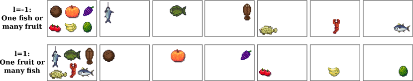
Figure 4: Example of a dataset an AFC $\kappa=6$. The “fruit” features are concentrated in one image for class $l=-1$ but spread out over six images for $l=1$ (vice versa for the “fish” features). Each individual feature is not indicative of the class as it appears exactly once in each class. Nevertheless, Arthur and Merlin can exchange “fruits” to indicate “$l=1$” and “fish” for “$l=-1$”. The images where this strategy fails or can be exploited by Morgana are the two images on the left. Applying 2.8, we get $\epsilon_{M}=\frac{1}{7}$ and the set $D^{\prime}$ corresponds to all images with a single feature. Restricted to $D^{\prime}$, the features determine the class completely.

2.2 Merlin-Arthur Classification

For a feature classifier $A$ (Arthur) and two feature selectors $M$ (Merlin) and $\widehat{M}$ (Morgana) we define

$$E_{M,\widehat{M},A}:=\mathopen{}\left\{x\in D\,\middle|\,A\mathopen{}\left(M(\mathbf{x})\right)\mathclose{}\neq c(\mathbf{x})~{}\vee A\mathopen{}\left(\widehat{M}(\mathbf{x})\right)\mathclose{}=-c(\mathbf{x})\right\}\mathclose{}$$ (3)

as the set of data points for which Merlin fails to convince Arthur of the correct class or Morgana is able to trick him into returning the wrong class, in short, the set of points where Arthur fails. We can now state the following theorem connecting the competitive game between Arthur, Merlin and Morgana to the class conditional entropy.

Theorem 2.8.

[Min-Max] Let $M\in\mathcal{M}(D)$ be a feature selector and let

$$\epsilon_{M}=\min_{A\in\mathcal{A}}\max_{\widehat{M}\in\mathcal{M}}\,\mathbb{P}_{\mathbf{x}\sim\mathcal{D}}\mathopen{}\left[\mathbf{x}\in E_{M,\widehat{M},A}\right]\mathclose{}.$$

Then a set $D^{\prime}\subset D$ with $\mathbb{P}_{\mathbf{x}\sim\mathcal{D}}\mathopen{}\left[\mathbf{x}\in D^{\prime}\right]\mathclose{}\geq 1-\epsilon_{M}$ exists such that for $\mathcal{D}^{\prime}=\mathcal{D}|_{D^{\prime}}$ we have

$$Q_{\mathcal{D}^{\prime}}(M)=1,\quad\text{thus}\quad H_{\mathbf{x},\mathbf{y}\sim\mathcal{D}^{\prime}}(c(\mathbf{y})\;|\;\mathbf{y}\in M(\mathbf{x}))=0.$$

The proof is in Appendix B. This theorem states that if Merlin’s strategy allows Arthur to classify almost perfectly, i.e., small $\epsilon_{M}$, then there exists a set that covers almost the entire original dataset and on which the class entropy conditioned on the selected features is zero. Note that these guarantees are for the set $D^{\prime}$ and not the original set $D$. A bound for the set $D$, such as $Q_{\mathcal{D}}(M)\geq 1-\epsilon_{M},$ is complicated by a factor we call asymmetric feature correlation (AFC).

2.3 Asymmetric Feature Correlation:

AFC describes a possible quirk of datasets, where a set of features is strongly concentrated in a few data points in one class and spread out over almost all data points in another. We give an illustrative example in Figure 4. If a data space $\mathfrak{D}$ has a large AFC $\kappa$, Merlin can use features that individually appear equally in both classes (low precision) to indicate the class where they are spread over almost all points. Morgana can only fool Arthur in the other class where these features are highly concentrated, thus only in a few data points. This ensures a small $\epsilon_{M}$ even with uninformative features.

For a set of features $F\subset D_{p}$ we define

$$F^{\ast}:=\mathopen{}\left\{\mathbf{x}\in D~{}|~{}\exists~{}\mathbf{z}\in F:\mathbf{z}\subseteq\mathbf{x}\right\}\mathclose{},$$

the set of all datapoints that contain a feature from $F$.

Definition 2.9 (Asymmetric feature correlation).

Let $(D,\mathcal{D},c)$ be a two-class data space, then the asymmetric feature correlation $\kappa$ is defined as

$$\kappa=\max_{l\in\mathopen{}\left\{-1,1\right\}\mathclose{}}\max_{F\subset D_{p}}\mathbb{E}_{\mathbf{y}\sim\mathcal{D}_{l}|_{F^{*}}}\mathopen{}\left[\max_{\begin{subarray}{c}\mathbf{z}\in F\\ \text{s.t. }\mathbf{y}\in\mathbf{z}\end{subarray}}\kappa_{l}(\mathbf{z},F)\right]\mathclose{}$$

with

$$\kappa_{l}(\mathbf{z},F)=\frac{\mathbb{P}_{\mathbf{x}\sim\mathcal{D}_{-l}}\mathopen{}\left[\mathbf{z}\subseteq\mathbf{x}\,\middle|\,\mathbf{x}\in F^{*}\right]\mathclose{}}{\mathbb{P}_{\mathbf{x}\sim\mathcal{D}_{l}}\mathopen{}\left[\mathbf{z}\subseteq\mathbf{x}\,\middle|\,\mathbf{x}\in F^{*}\right]\mathclose{}}.$$

We derive this expression in more detail in Section B.3, but give an intuition here. The probability $\mathbb{P}_{\mathbf{x}\sim\mathcal{D}_{l}}\mathopen{}\left[\mathbf{z}\subseteq\mathbf{x}\,\middle|\,\mathbf{x}\in F^{*}\right]\mathclose{}$ for $\mathbf{z}\in F$ is a measure of how correlated the features are. If all features appear in the same datapoints this quantity takes a maximal value of 1 for each $\mathbf{z}$. If no features share the same datapoint the value is minimally $\frac{1}{\mathopen{}\left|F\right|\mathclose{}}$ for the average $\mathbf{z}$. The $\kappa_{l}(\mathbf{z},F)$ thus measures the difference in correlation between the two classes. In the example in Figure 4 the worst-case $F$ for $l=-1$ correspond to the “fish” features and $\kappa_{l}(\mathbf{z},F)=6$ for each feature. To take an expectation over the features $\mathbf{z}$ requires a distribution, so we take the distribution of datapoints that have a feature from $F$, i.e. $\mathbf{y}\sim\mathcal{D}_{l}|_{F^{*}}$, and select the worst-case feature from each datapoint. Then we maximise over class and the possible feature sets $F$. Since in Figure 4, the “fish” and “fruit” features are the worst case for each class respectively, we arrive at an AFC of 6.

Though it is difficult to calculate the AFC for complex datasets, we show that it can be bounded above by the maximum number of features per data point in $D$.

Lemma 2.10.

Let $\mathfrak{D}$ be a two-class data space with AFC of $\kappa$. Let $K=\max_{\mathbf{x}\in D}\,\mathopen{}\left|\mathopen{}\left\{\mathbf{z}\in D_{p}\,|\,\mathbf{z}\subseteq\mathbf{x}\right\}\mathclose{}\right|\mathclose{}$ be the maximum number of features per data point. Then $\kappa\leq K.$

We prove this in Appendix B. The number $K$ depends on the type of features one considers, e.g. for image data a rectangular cutout of given size, then $K\sim d$, when any subset of pixels is allow then $K\sim 2^{d}$. See also Appendix B for an example dataset with an exponentially bad AFC.

2.4 Realistic Algorithms and Relative Success Rate

In 2.8, we make use of a perfect Morgana. For complex classifiers this implies exhaustive search, which is indeed possible for low-dimensional data often used in recruitment and criminal justice, where interpretability is crucial. Consider the UCI Census Income dataset Dua & Graff (2017) with 14 dimensions. When restricting features to a maximal size of seven, the search space is at most $\binom{14}{7}=3432$, within range for exhaustive search. Contrary to this, modelling the UCI data distribution explicitly is still an involved task, and when done incorrectly, leads to incorrect explanations Frye et al. (2020).

However, we also aim to apply our setup to high-dimensional datasets, where exhaustive search is not possible. It turns out we can relax the requirement for Morgana to play optimally in two important ways: (i) She only has to find the features that can also be found by Merlin (ii) She only has to do so with a success rate comparable to Merlin.

Definition 2.11 (Relative Success Rate).

Let $\mathfrak{D}=(D,\mathcal{D},c)$ be a two-class data space. Let $A\in\mathcal{A}$ and $M,\widehat{M}\in\mathcal{M}(D)$. Then the relative success rate $\alpha$ of $\widehat{M}$ with respect to $A,M$ and $\mathfrak{D}$ is defined as

$$\alpha:=\min_{l\in\mathopen{}\left\{-1,1\right\}\mathclose{}}\frac{\mathbb{P}_{\mathbf{x}\sim\mathcal{D}_{-l}}\mathopen{}\left[A(\widehat{M}(\mathbf{x}))=l\,|\,\mathbf{x}\in F_{l}^{\ast}\right]\mathclose{}}{\mathbb{P}_{\mathbf{x}\sim\mathcal{D}_{l}}\mathopen{}\left[A(M(\mathbf{x}))=l\,|\,\mathbf{x}\in F_{l}^{\ast}\right]\mathclose{}},$$

where $F_{l}:=\mathopen{}\left\{\mathbf{z}\in D_{p}\,|\,\mathbf{z}\in M(D_{l}),A(\mathbf{z})=l\right\}\mathclose{}$.

The set $F_{l}$ is the set of all features that Merlin uses in class $l$ to successfully convince Arthur. Thus we only evaluate Morgana’s performancy on datapoints where she can in principle find one of Merlin’s features. The question is then how the context of the other features makes this computationally easier or harder. We discuss this idea in more depth in Appendix B and give a worst-case example in Figure 13. We argue that realistically, we can assume a large $\alpha$ when using an algorithm for Morgana that is at least as powerful as the one for Merlin. Together with the AFC, this allows us to state the following theorem.

Theorem 2.12.

Let $\mathfrak{D}=(D,\mathcal{D},c)$ be a two-class data space with AFC of $\kappa$ and class imbalance $B$. Let $A\in\mathcal{A}$, and $M,\widehat{M}\in\mathcal{M}(D)$ such that $\widehat{M}$ has a relative success rate of $\alpha$ with respect to $A,M$ and $\mathfrak{D}$. Define

1. Completeness:

$$\min\limits_{l\in\mathopen{}\left\{-1,1\right\}\mathclose{}}\mathbb{P}_{\mathbf{x}\sim\mathcal{D}_{l}}\mathopen{}\left[A\mathopen{}\left(M(\mathbf{x})\right)\mathclose{}=c(\mathbf{x})\right]\mathclose{}\geq 1-\epsilon_{c},$$

2. Soundness

$$\max\limits_{l\in\mathopen{}\left\{-1,1\right\}\mathclose{}}\mathbb{P}_{\mathbf{x}\sim\mathcal{D}_{l}}\mathopen{}\left[A\mathopen{}\left(\widehat{M}(\mathbf{x})\right)\mathclose{}=-c(\mathbf{x})\right]\mathclose{}\leq\epsilon_{s}.$$

Then it follows that

$$Q_{\mathcal{D}}(M)\geq 1-\epsilon_{c}-\frac{\kappa\alpha^{-1}\epsilon_{s}}{1-\epsilon_{c}+\kappa\alpha^{-1}B^{-1}\epsilon_{s}}.$$

The proof is provided in Appendix B. The core assumption we make when comparing our lower bound with the measured average precision in Section 3 is the following:

Assumption 2.13.

The AFC $\kappa$ of $\mathfrak{D}$ and the relative success rate $\alpha$ of $\widehat{M}$ w.r.t. A, M, $\mathfrak{D}$ are $\mathcal{O}(1)$.

As of yet, we cannot confirm whether a dataset has small AFC. But we conjecture that even if it contains a feature set that realises large AFC, finding it is a computationally hard task for Merlin. We leave this open for further research.

Finitely Sampled and Biased Dataset

We usually have access to only finitely many samples of a dataset. Additionally, the observed samples can be biased as compared to the true distribution. We prove bounds for both cases in Section B.5. We show that any exchanged feature is either informative, or it is incorrectly represented in the dataset—thus highlighting the bias!

In conclusion, the theoretical results presented show that (i) For optimal feature selectors and classifiers, we can guarantee highly informative features without the need to model the data distribution, see 2.8. (ii) For suboptimal agents we can still assure informative features as long as the success probability of Morgana is comparable to the one of Merlin, see 2.12. (iii) We can certify feature quality with measurable quantities soundness and completeness.

3 Numerical Implementation

We illustrate the merit of our framework with experiments on the UCI Census Income dataset and on the MNIST handwritten digits dataset (LeCun et al., 1998).

First, we describe how to train the agents Arthur, Merlin, and Morgana in a general $n$-class interactive learning setting for image data of dimension $d$, where $n,d\in\mathbb{N}$. We explain in Section A.3 why we chose a multi-class neural network for Arthur and compare with the approaches of Chang et al. (2019) and Anil et al. (2021). The training process for tabular data, like the Census dataset, is equivalent and a detailed overview is provided in the appendix.

Arthur is modelled by a feed-forward neural network. He returns a probability distribution over his possible answers, so let $A:[0,1]^{d}\rightarrow[0,1]^{(n+1)}$, corresponding to the probabilities of stating a class or “I don’t know”. The provers select a set $S$ of at most $k$ pixels from the image via a mask $\mathbf{s}\in B_{k}^{d}$, where $B_{k}^{d}$ is the space of $k$-sparse binary vectors of dimension $d$. A masked image $\mathbf{s}\cdot\mathbf{x}$ has all its pixels outside of $S$ set to a baseline or a random value. We define the Merlin-loss $L_{M}$ as the cross-entropy loss with regard to the correct class, whereas the Morgana-loss $L_{\widehat{M}}$ considers the total probability of either answering the correct class or the “I don’t know” option, so

$$L_{M}(A,\mathbf{x},\mathbf{s})=-\log\mathopen{}\left(A(\mathbf{s}\cdot\mathbf{x})_{c(\mathbf{x})}\right)\mathclose{}\quad\text{and}\quad L_{\widehat{M}}(A,\mathbf{x},\mathbf{s})=-\log\mathopen{}\left(A(\mathbf{s}\cdot\mathbf{x}))_{0}+A(\mathbf{s}\cdot\mathbf{x})_{c(\mathbf{x})}\right)\mathclose{}.$$

The total loss for Arthur is then

$$L=\mathbb{E}_{\mathbf{x}\sim\mathcal{D}}[L(\mathbf{x})]\quad\text{where}\quad L(\mathbf{x})=(1-\gamma)L_{M}(A,\mathbf{x},M(\mathbf{x}))+\gamma L_{\widehat{M}}(A,\mathbf{x},\widehat{M}(\mathbf{x})),$$

and $\gamma\in[0,1]$ is a tunable parameter. In our experiments, we choose $\gamma>0.5$ since we always want to ensure good soundness. We compare different $\gamma$ in Appendix C. Note that Merlin wants to minimise $L_{M}$, whereas Morgana aims to maximise $L_{\widehat{M}}$. In an ideal world, they would solve

$$M(\mathbf{x})=\operatorname*{arg\,min}_{\mathbf{s}\in B_{k}^{d}}L_{M}(A,\mathbf{x},\mathbf{s})\quad\text{and}\quad\widehat{M}(\mathbf{x})=\operatorname*{arg\,max}_{\mathbf{s}\in B_{k}^{d}}L_{\widehat{M}}(A,\mathbf{x},\mathbf{s}).$$ (4)

The above solutions can be obtained either by solving the optimisation problem (Frank-Wolfe solver (Macdonald et al., 2022)) or by using NNs to predict the solutions (UNet architecture). We kept our training routine simple by looping over the three agents and describe the details of the training algorithm and architectures in Appendix C.

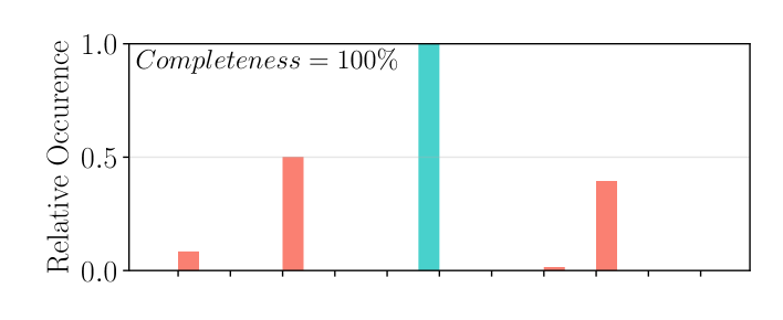
1a) $\beta=0$ $\gamma=0$	1b) $\beta=3.5$ $\gamma=0$
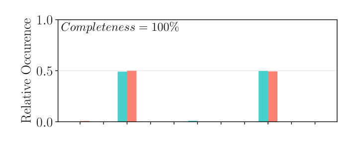
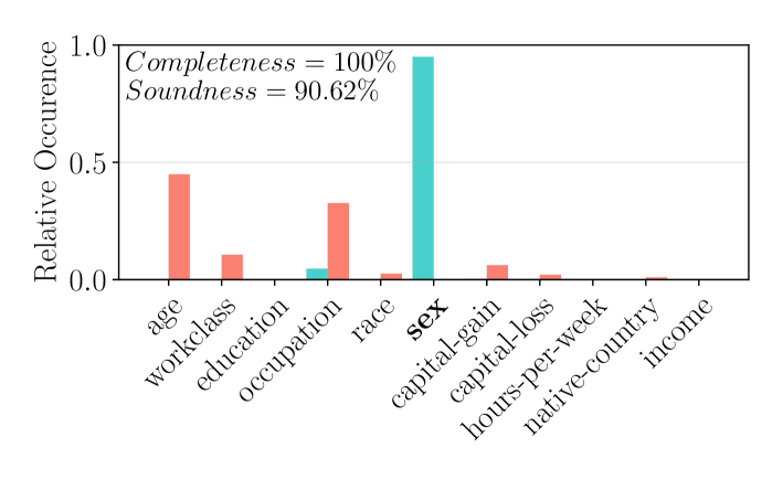
2a) $\beta=3.5$ $\gamma=0.67$	2b) $\beta=10$ $\gamma=0.67$

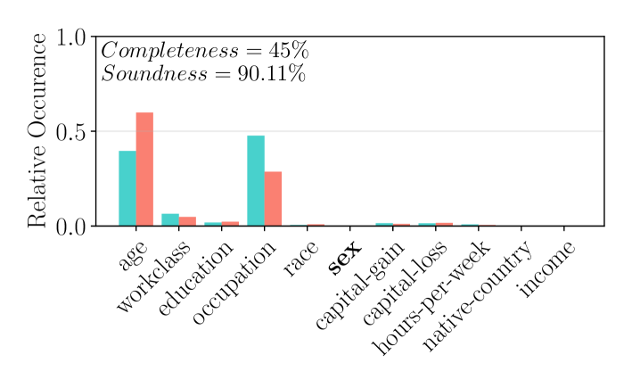
Figure 5: Hiring only men while hiding “sex” as the explanation. 1. No soundness is required ($\gamma=0$). a) Merlin has no punishment for showing “sex” ($\beta=0$). He sends Arthur the “sex” feature and they discriminate successfully (high completeness). b) Merlin is incentivised not to use “sex” ($\beta>0$). He successfully communicates the “sex” to Arthur via different features, here “hours per week” and “education”. Morgana can exploit this strategy with the same features switched. 2. High soundness is now required ($\gamma=0.67$). Merlin either a) shows the “sex” feature despite the punishment ($\beta=3.5$) and achieves high completeness, or b) hides the “sex” feature ($\beta=10$) and reduces completeness below 50%, which corresponds to no discrimination.

3.1 Preventing Manipulation

Since existing XAI algorithms have no guarantees, they cannot exclude the possibility for manipulation. Indeed, arbitrarily changing the interpretation by slightly modifying the classifier has been demonstrated for many XAI approaches.

Slack et al. fool LIME and ShAP by making use of the fact that these methods sample off-manifold evaluations of the classifier. We are robust against this approach, since the Merlin-Arthur classifier only takes on-manifold inputs.

Dimanov et al., Heo et al. and Anders et al. optimise manipulated classifier networks to give the desired explanations by penalising any deviation. The equivalent for our setup is to put a penalty on Merlin to hide the true (potentially biased) explanations in the exchanged features. This scheme is unsuccessful for a Merlin-Arthur classifier as we show numerically that either: (i) The bias becomes visible, (ii) Morgana can exploit the setup, i.e., soundness is low or (iii) the completeness, i.e., prediction accuracy, drops.

We demonstrate this on a modified UCI Census Income dataset. We train a classifier to discriminate by “sex”—one of the remaining 12 features. We change the Merlin-loss to

$$L^{\prime}_{M}(A,\mathbf{x},\mathbf{s}):=L_{M}(A,\mathbf{x},\mathbf{s})+\beta\mathopen{}\left\|\mathbf{s}_{\text{sex}}\right\|\mathclose{},$$

where $\beta>0$, to train Merlin to hide the sensitive “sex” feature. We then train the Merlin-Arthur classifier to accept only men and set $k=1$ to only send one feature. We compare a setup where soundness is ignored to one where we choose $\gamma$ such that a soundness of at least 90% is achieved.

The results are illustrated in Figure 5. When soundness is ignored ($\gamma=0$), setting $\beta=3.5$ causes Merlin to hide the “sex” feature and communicate “sex” via selecting “education” for men, “working hours” for women. When soundness is required ($\gamma=0.67$), Merlin starts to reveal the “sex” feature again. Increasing the penalty to $\beta=10$, causes him to hide “sex”, but now the prediction accuracy reduces to $0.45$, i.e., close to chance and thus ceasing the discrimination. When high soundness is required, Merlin is unable to both discriminate and hide his bias.

3.2 Evaluation of Theoretical Bounds

Low-dimensional datasets can be used to evaluate the mutual information bounds since for small features there are multiple datapoints that contains them and the ground truth information of the feature can be estimated.

We evaluate our framework on the MNIST dataset restricted to two classes. We use 2.12 and 2.13 to calculate a lower bound on the average precision $Q_{\mathcal{D}}(M)$ for two different pairs of classes. We compare three different setups of feature selectors, one with Frank-Wolfe optimisers (Opt), one where Merlin is a UNet and Morgana an optimiser (Hybrid), and one where we use UNets for both (Net). We show the comparison between our theoretical prediction and the empirical estimate of average precision in Figure 6 and find good agreement. Our lower bound is always below the empirical estimatate, which is evidence that 2.13 is correct.

In Figure 6, we see that the lower bound is tight for larger masks, but drops off when $k$ is small. One reason is that for small masks, Arthur tends to give up on one of the classes, while keeping the completeness in the other class high. Since the bound considers the minimum over both classes, it becomes pessimistic. Regularising Arthur to maintain equal completeness is a potential solution, but this requires global information that for a single batch can only be roughly estimated.

When Merlin and Morgana are realised by the same method (both optimisers or NNs), the bound is the tightest. In our hybrid approach, Merlin is at a disadvantage, since he needs to learn a general rule on the training set to select good features, whereas Morgana can optimise directly on the test set during evaluation. In Appendix C Figure 15, we show error bars sampled over 10 training runs. The training results have greater variance for small masks. This is because there is no perfect strategy for Arthur, who cycles between good completeness and soundness.

compat=1.15

		Opt	Hybrid	Net	Example Features
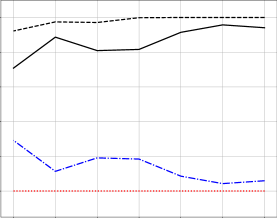
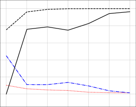
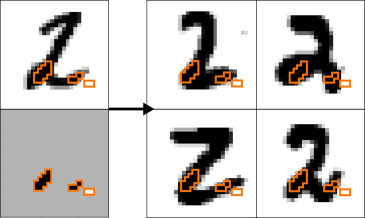
“2” vs “4”						$\#$Images/Feature
“6” vs “9”
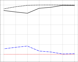
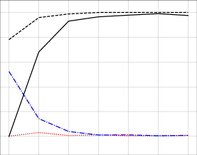
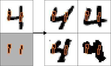
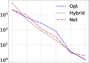
		$k$	$k$	$k$		$k$

Figure 6: Left: For four different setups of Merlin and Morgana, we compare the lower bound on $Q_{\mathcal{D}}(M)$ with the experimental results on the MNIST dataset. The top row is for the labels $\mathopen{}\left\{\text{``2''},\text{``4''}\right\}\mathclose{}$, and the bottom row for $\mathopen{}\left\{\text{``6''},\text{``9''}\right\}\mathclose{}$. The bound is tight for large masks, but loosens sharply for very small mask sizes $k$. Middle: Examples of the features selected by Merlin for two images. For the “4” feature, there are 13 images in MNIST that share it, all of them of class “4” (we show four here). For the “2” there are 16 images, all of them in “2”. Right: The average number of images found for a feature selected by Merlin. These images were used to estimate $Q_{\mathcal{D}}(M)$.

4 Discussion

It has been shown in Macdonald et al. (2020) that finding informative features for NN classifiers is $\mathsf{NP}$-hard. Thus, any efficient algorithm is a heuristic. Training a Merlin-Arthur classifier is a heuristic as well, as we are not guaranteed to converge to an equilibrium with informative features. However, the framework allows us to verify whether we succeeded by evaluating completeness and soundness on the test dataset. Without it, even just confirming that a given feature is informative is typically an involved task and requires a provably good model of the data distribution Frye et al. (2020); Aas et al. (2021); Wäldchen et al. (2022). An interactive classification setup circumvents these problems. We comment further on this topic in Appendix A.

We can draw a connection between training Arthur against Morgana and Adversarial Robustness (Goodfellow et al., 2014). Consider the generation of adversarial examples : $\bm{\delta}^{\ast}=\operatorname*{arg\,min}_{\mathopen{}\left\|\bm{\delta}\right\|\mathclose{}\leq\epsilon}L(\mathbf{x}+\bm{\delta}),$ a perturbation that changes the classification but is imperceptible to humans. The intuition behind adversarial robustness is that minuscule changes should not change the classifier decision. Likewise, the intuition behind soundness, i.e., robustness with respect to Morgana, is that hiding parts of an object should not convince the classifier of a different class. At most, one could hide the whole object, which is reflected in the “Don’t know!” option. In this sense, soundness is a natural counterpart to adversarial robustness and should be expected of classifiers that generalise to partially hidden objects.

AFC seems to be more generally relevant to interactive interpretability. In Yu et al. (2019) a prover sends part of an image to a cooperative verifier and the left-over to an adversarial classifier. The goal is to allow correct classification for the cooperator and prevent it for the adversary. However, as in our example in Figure 4, the prover can use completely uninformative features (“fish” and “fruit”) and the adversary is unable to exploit this except for a small number of image, proportional to the AFC. We explain this in more detail in Section A.4.2.

5 Impact & Limitations

High completeness and soundness can be mandated for commercial classifiers, e.g., in the context of hiring decisions with past decisions by the Merlin-Arthur classifier as ground truth. An auditor should use their own Morgana to verify sufficient soundness. If so, the features by Merlin are verifiably the basis of the hiring decisions can be inspected for protected attributes, e.g., race, sex or attributes that strongly correlate with them (Mehrabi et al., 2021).

However, simply identifying features with high mutual information does not necessarily point to causal mechanisms, since they can include spurious correlations. For our experiments on the UCI dataset the removed features “marital status” and “relationship” are correlated with sex and thus can be used by Merlin to communicate “sex” to Arthur when included, see Section C.4. It is up to society to determine whether the exchanged features constitute discrimination. This is a problem shared by most interpretability tools, however, there has been progress to adapt interactive classification to find causal features Chang et al. (2020).

Our theoretical results are so far only formulated for two classes. We expect them to be extendable to a $n$-class setting, but leave this to further research. It remains to be seen whether our proposed training setup can be extended to more involved datasets while retaining stability. So far, we have kept the training routine straightforward and simple. Similar to GAN-training, which is notoriously difficult (Roth et al., 2017; Wiatrak et al., 2019), there is potential for further sophistication.

6 Conclusion

We extend the framework of adversarial interactive classifiers to provide quantitative bounds on the mutual information of the selected features. These bounds are in terms of the average precision and ultimately in terms of measurable criteria such as completeness and soundness. We also extend our method beyond the assumption of feature independence that is common in such settings by introducing the notion of Asymmetric Feature Correlation that captures the necessary aspect of the dependence among the features. Finally, we evaluate our results on the UCI Census Income and MNIST datasets and show that the Merlin-Arthur classifier can prevent manipulation that has been demonstrated for other XAI methods and that our theory matches well with our numerical results.

Appendix A Conceptual Overview

Formal interpretability faces two hurdles: a complexity barrier, as well as a modelling problem. Here, we further explain these challenges and how we overcome them. Furthermore, we show for two alternative interactive classification setups with an adversary, the debate setup (Irving et al., 2018) and the adversarial classifier setup Yu et al. (2019); Dabkowski & Gal (2017), that they cannot be used to derive bounds with the same generality as in our work. Instead, it would require stronger assumptions on either the classifier or the data space to exclude our counterexamples. We also compare our architecture in detail with that proposed in  Chang et al. (2019) and Anil et al. (2021) and provide an explanation for the differences.

A.1 Computational Complexity

Prime Implicant Explanations (Shih et al., 2018), a concept from logical abduction, can be efficiently computed for simple classifiers like decision trees (Izza et al., 2020) and monotonic functions (Marques-Silva et al., 2021). This concept has been extended to NNs (Ignatiev et al., 2019) in the form of probabilistic prime implicants, which correspond to features with high precision. However, it has been shown that even approximating small implicants within any non-trivial factor is $\mathsf{NP}$-hard (Waeldchen et al., 2021) for networks of two layers or more. In Blanc et al. (2021), the authors construct an algorithm that circumvents these hardness results by further relaxation of the problem. While this is a noteworthy theoretical breakthrough, the polynomial bound on the feature size grows so quickly with the dimension of the data space that the algorithm does not guarantee useful features for real-world data. For reasonably sized images, one would get guarantees only for features that cover the whole image.

We circumvent the hardness of this problem using a method that is very typical of Deep Learning: Use a heuristic and verify success afterwards! Our approach can be put alongside the regular training of classifiers, which is a theoretically hard problem as well. A heuristic like Stochastic Gradient Descent is not a priori guaranteed to produce a capable classifier. However, we can check the success of the procedure by evaluating the accuracy on a test dataset. In our case, training the Merlin-Arthur classifier is not guaranteed to converge to an equilibrium with informative features. But we can check whether this is the case via the test dataset, where soundness and completeness take the role of the accuracy.

A.2 Modelling the True Data Distribution

We introduce Merlin-Arthur classification as it provides us a way to measure the feature quality via the completeness and soundness values over a test dataset. This would not be necessary if we could directly measure the feature quality over the dataset (though it would still be faster than measuring every individual feature). The reason we need the Merlin-Arthur setup is that for general datasets the conditional entropy

$$H_{\mathbf{y}\sim\mathcal{D}}(c(\mathbf{y})\,|\,\mathbf{z}\subseteq\mathbf{y})=H_{\mathbf{y}\sim\mathcal{D}|_{\mathbf{z}\subseteq\mathbf{y}}}(c(\mathbf{y})),$$

is difficult to measure, since we do not generally know the conditional distribution $\mathcal{D}|_{\mathbf{z}\subseteq\mathbf{y}}$. This measurement is possible for MNIST for small features since the dataset is very simple. However, for more complex data, a feature which is large enough to be indicative of the class will in all likelihood not appear more than once in the same dataset. We will now discuss some existing approaches that aim to approximate the conditional data distribution and what problems they face.

Modelling the conditional data distribution has been pursued in the context of calculating Shapley values. These are a different interpretability method based on characteristic functions from cooperative game theory that assign a value to every subset of a number of features (Shapley, 2016). We will shortly discuss the approach proposed in Lundberg & Lee (2017), where features correspond to partial vectors supported on sets.

Let $f:[0,1]^{d}\rightarrow\mathopen{}\left\{-1,1\right\}\mathclose{}$ be a classifier function. Then we can naturally define a characteristic function $\nu_{f,\mathbf{x}}:\mathcal{P}([d])\rightarrow[-1,1]$ as

$$\nu_{f,\mathbf{x}}(S)=\mathbb{E}_{\mathbf{y}\sim\mathcal{D}}\mathopen{}\left[f(\mathbf{y})\,|\,\mathbf{y}_{S}=\mathbf{x}_{S}\right]\mathclose{}=\int f(\mathbf{y}_{S},\mathbf{x}_{S^{c}})d\mathbb{P}_{\mathbf{y}\sim\mathcal{D}}(\mathbf{y}_{S^{c}}~{}|~{}\mathbf{y}_{S}=\mathbf{x}_{S}).$$

The Shapley value for the input component $x_{i}$ is then defined as

$$\text{Shapley Value}(x_{i})=\frac{1}{d}\sum_{S\subseteq[d]\setminus\mathopen{}\left\{i\right\}\mathclose{}}\begin{pmatrix}d-1\\ \mathopen{}\left|S\right|\mathclose{}\end{pmatrix}^{-1}(\nu_{f,\mathbf{x}}(S\cup\mathopen{}\left\{i\right\}\mathclose{})-\nu_{f,\mathbf{x}}(S)).$$

In Macdonald et al. (2022), the characteristic function is instead used to define a feature selection method as

$$\mathbf{x}_{S^{*}}\quad\text{where}\quad S^{*}=\operatorname*{arg\,min}_{\mathopen{}\left|S\right|\mathclose{}\leq k}\,\operatorname*{dist}(\nu([d]),\nu(S)),$$

where $k\in[d]$ is a cap on the set size and $\operatorname*{dist}$ is an appropriate distance measure.

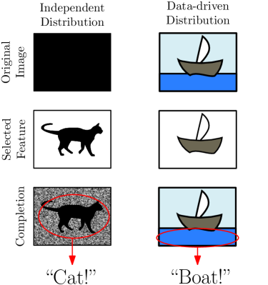
Figure 7: Different failure modes of unrepresentative distributions. Left: Independent, random inpainting, similar to Macdonald et al. (2019). From a black image, the shape of a cat is selected, and the rest is filled with uniform noise. The shape of a cat is detected by a classifier. Right: Data-driven inpainting, similar to Agarwal & Nguyen (2020). The image of a ship is given and the ship-feature is selected. The data driven distribution inpaints the water back into the image, since in the dataset, ships are always on water. The faulty classifier that relies on the water feature is undetected, as the ship-feature indirectly leads to the correct classification.

As in our setup, the problem is that these approaches depend on how well the conditional probability $\mathbb{P}_{\mathbf{y}\sim\mathcal{D}}(\mathbf{y}_{S^{c}}~{}|~{}\mathbf{y}_{S}=\mathbf{x}_{S})$ is modelled. Modelling the data distribution incorrectly makes it possible to manipulate many existing XAI-methods. This is done by changing the classifier in such a way that it gives the same value on-manifold, but arbitrary values off-manifold. To get feature-based explanations independent of the off-manifold behaviour, one needs to model the data manifold very precisely (Aas et al., 2021; Dombrowski et al., 2019). The authors of Anders et al. (2020); Heo et al. (2019) and Dombrowski et al. (2019) demonstrate this effect for existing techniques, such as sensitivity analysis, LRP, Grad-Cam, IntegratedGradients and Guided Backprop. They are able to manipulate relevance scores at will and demonstrate how this can be used to obfuscate discrimination inside a model. LIME and SHAP can be manipulated as well (Slack et al., 2020) by using a classifier that behaves differently outside off-distribution if the wrong distribution for the explanation. For RDE (Macdonald et al., 2019) it is assumed that features are independent and normally distributed, and it was demonstrated that the off-manifold optimisation can create new features that weren’t in the original image (Wäldchen et al., 2022).

We now discuss two approaches proposed to model the data distribution and why each leads to a different problem by under- or over-representing correlation in the data respectively.

Independent distribution:

Which means that the conditional probability is modelled as

$$\mathbb{P}_{\mathbf{y}\sim\mathcal{D}}(\mathbf{y}_{S^{c}}~{}|~{}\mathbf{y}_{S}=\mathbf{x}_{S})=\prod_{i\in S^{c}}p(y_{i}),$$

where $p(y_{i})$ are suitable probability densities on the individual input components. This approach has been used in Fong & Vedaldi (2017) and Macdonald et al. (2022), where optimisers are employed to find small features that maximise the classifier score. In fact, Macdonald et al. (2022) has to make a new approximation of the data distribution in every layer and it has been shown that for neural networks one cannot do much better than applying either this or sampling Macdonald & Wäldchen (2022). It was highlighted in Wäldchen et al. (2022) how this approach, when modelling the data distribution incorrectly, will create artificial new features that were not present in the original image. Employing an optimisation method with this distribution can result in masks that generate new features that were not present in the original image. We illustrate this problem in Figure 7. Cutting a specific shape out of a monochrome background will with high likelihood result in an image where this shape is visible. If the distribution was true, a monochrome shape would likely lead to an inpainting that is monochrome in the same colour, destroying the artificial feature. But an independent distribution under-represents these reasonable correlations.

Taking a data-determined distribution via generative model:

Which means that the conditional probability is modelled as

$$\mathbb{P}_{\mathbf{y}\sim\mathcal{D}}(\mathbf{y}_{S^{c}}~{}|~{}\mathbf{y}_{S}=\mathbf{x}_{S})=G(\mathbf{y}_{S^{c}};\mathbf{x}_{S}),$$

where $G$ is a suitable generative model. Generative models as a means to approximate the data distribution in the context of explainability have been proposed in a series of publications (Agarwal & Nguyen, 2020; Chang et al., 2018; Liu et al., 2019; Mertes et al., 2020). This setup introduces a problem. If the network and the generator were trained on the same dataset, the biases learned by the classifier will appear might be learned by the generator as well (see Figure 7 for an illustration)! The important cases will be exactly the kind of cases that we will not be able to detect. If the generator has learned that horses and image source tags are highly correlated, it will inpaint an image source tag when a horse is present. This allows the network to classify correctly, even when the network only looks for the tag and has no idea about horses. The faulty distribution over-represents correlations that are not present in the real-world data distribution.

A.3 Design of the Three-Way Game

The basic setup for a prover-verifier game for classification was proposed by Chang et al. with a verifier, a cooperative prover and an adversarial prover for one specific class. The verifier either accepts the evidence for the class or rejects it. Both provers try to convince the verifier, the cooperative prover operates on data from the class, the adversary on data from outside the class. The authors suggest that the way to scale to multiple classes is to have three agents for every class.

In our work, we combine the agents over all classes, to have a single verifier (Arthur), cooperator (Merlin), and adversary (Morgana). The verifier rejecting all the classes in their paper corresponds to our “Don’t know!” option. In our design in Section 3, we make the implicit assumption that the class of the datapoint is unique. Combining the verifiers gives us a numerical advantage for two reasons. First, since a lot of lower-level concepts (e.g. edges and corners for image data) are shared over classes, the lower levels of the neural network benefit by being trained on more and more diverse data. Second, we can leverage the knowledge that the class is unique by outputting a distribution over classes (and “Don’t know!”). Both lines of reasoning are standard for deep learning Bridle (1989).

Anil et al. further combine Merlin and Morgana into a single prover that probabilistically produces a certificate for a random class. This has the advantage that it allows for further weight-sharing among the provers. However, the probabilistic nature of the certificate is also a disadvantage. The probability of generating the certificate for the correct class is the inverse of the total number of classes. When applied after training, one only occasionally gets a valid classification. In our case, we can always use Merlin together with Arthur to obtain the correct class together with an interpretable feature

A.4 Alternative setups

Here we discuss alternatives to the Merlin-Arthur setup. Both these alternatives present an interactive classification setup as well. However, we show that they cannot prove bounds with the same generality as we have proven.

A.4.1 Debate Model

The debate setting introduced in Irving et al. (2018) is an intriguing alternative to our proposed setup. However, we are now going to present an example data space on which, in debate mode, Arthur and Merlin can cooperate perfectly without using informative features. For this, we use the fact that in the debate setting, Arthur receives features from both Merlin and Morgana for each classification. Our example illustrates that the debate setting would need stronger requirements on either the data space or Arthur to produce results similar to ours.

Consider the following example of a data space $\mathfrak{D^{\text{ex}}}$, illustrated in Figure 8.

Example A.1.

Given $n\in\mathbb{N},n\geq 4$, we define the data space $\mathfrak{D^{\text{ex}}}=(D,\mathcal{D},c)$ with

• $D=D_{-1}\cup D_{1}\quad\text{where}\quad D_{s}=\bigcup^{n}_{k=1}[2k+s,2k]$

• for $T\in\mathcal{P}(D):\mathcal{D}(T)=\frac{\mathopen{}\left|T\right|\mathclose{}}{N}$,

• $c(\mathbf{x})=\begin{cases}-1&\mathbf{x}\in D_{-1}\\ 1&\mathbf{x}\in D_{1}.\end{cases}$

None of the features in $D_{p}$ are informative of the class and the mutual information $I(c(x);\mathbf{z}\in\mathbf{x})$ for any $\mathbf{z}\in D_{p}$ is zero. Nevertheless, in a debate setting, Arthur can use the following strategy after receiving a total of two features from Merlin and Morgana

$$A(\mathopen{}\left\{\mathbf{z}_{1},\mathbf{z}_{2}\right\}\mathclose{})=\begin{cases}c(\mathbf{x}^{*})&\text{where}~{}\mathbf{x}^{*}=\operatorname*{arg\,max}_{\mathbf{x}\in D}\mathopen{}\left\|\mathbf{x}\right\|\mathclose{}_{1}~{}\text{s.t.}~{}\mathbf{z}_{1}\subseteq\mathbf{x},\mathbf{z}_{2}\subseteq\mathbf{x},\\ 0&\text{if}\not\exists\mathbf{x}\in D:\mathbf{z}_{1}\subseteq\mathbf{x},\mathbf{z}_{2}\subseteq\mathbf{x}.\end{cases}$$

This means he returns the class of the data point with the largest 1-norm that fits the presented features. But now Merlin can use the strategy

$$M(\mathbf{x})=\operatorname*{arg\,min}\limits_{\mathbf{z}}\mathopen{}\left\|\mathbf{z}\right\|\mathclose{}_{1}\,\text{s.t.}\,\mathbf{z}\subseteq\mathbf{x},$$

which returns the feature with the smaller 1-norm. It is easy to verify that no matter what Morgana puts forward, a feature with smaller or larger entry, nothing can convince Arthur of the wrong class. If she gives the same feature as Merlin, the data point will be correctly determined by Arthur. If she gives the other feature, the true data point is the unique one that has both features. Arthur’s strategy works as long as someone gives him the smaller feature.

a)	b)

Figure 8: Schematic of $\mathfrak{D^{\text{ex}}}$ as defined in A.1. a) The data space forms a bipartite graph, where every data point shares exactly one feature each with two data points from the opposite class. b) Classification on data point $[3,4]$. Merlin chooses the feature with the smallest 1-norm from this data point, so $[3,*]$. Arthur chooses the class of the data point with the highest 1-norm compatible with the presented features, so correctly $[3,4]$. Morgana can choose $\varnothing$, $[*,2]$ or $[3,*]$, but in all cases Arthur can correctly identify the original data point and return class $l=-1$.

In a setting where Arthur has to evaluate every feature individually, the best strategy that Arthur and Merlin can use achieves $\epsilon_{c}=\epsilon_{s}=\frac{1}{3}$, by making use of the asymmetric feature concentration. The AFC for $\mathfrak{D^{\text{ex}}}$ is $\kappa=2$, as can be easily verified by taking $F=\mathopen{}\left\{[*,2],[3,*],[*,6],[7,*]\right\}\mathclose{}$ in the definition of the AFC, see 2.9, and observing that they cover 4 data points in class $l=-1$ and only two in class $l=1$. But since the AFC-constant appears in the bound, the lower bound for $Q_{\mathcal{D}}(M)$ is $\frac{1}{6}$, well below the actual average precision of $\frac{1}{2}$.

This example demonstrates that Arthur and Merlin can successfully cooperate even with uninformative features, as long as Arthur does not have to classify on features by Morgana alone. This implies that to produce similar bounds as in our setup, the debate mode needs stronger restrictions on either the allowed strategies of Arthur or the structure of the data space, such that this example is excluded.

A.4.2 Adversarial Classifier

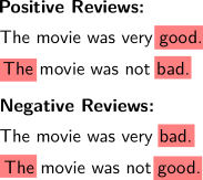
a)	b)

Figure 9: a) Illustration of the adversarial classification setup. Here, the prover selects a feature from the datapoint and sends it the cooperative verifier that decides the class. The datapoint without the feature is send to an adversary that also aims to decide the class. b) An example dataset that illustrates why this setup might fail to select for informative features. All selected features appear once in each class, thus have zero mutual information. Nevertheless, it is possible to classify perfectly with the selection, but not better than chance with the leftover.

An alternative interactive setup has been proposed in Yu et al. (2019); Dabkowski & Gal (2017), see Figure 9 a) for an illustration. In this setup a single prover selects a feature from the datapoint and sends it to a cooperative classifier that decides the class. The rest of the datapoint is sent to an adversarial classifier that also tries to classify correctly. The aim of the prover is to maximise the probability that the cooperator classifies correctly and that the adversary cannot perform much better than chance. This setup prevents cheating (in the sense illustrated in Figure 2), because selecting uninformative features would leave the informative features for the adversary. The optimal selections thus captures all the features that are sufficient to decide the class, whereas our Merlin-Arthur setup captures just the features that are necessary to decide the class. We should expect the latter set to be contained in the former.

Asymmetric Feature Correlation

We can analogously define completeness and soundness values corresponding to the classification accuracy of the cooperator and adversary respectively. But our argument laid out in Figure 4 still holds. Merlin can use the uninformative “fish” and “fruit” features to communicate the class to the cooperator. This works for all images except the two on the left with the many features. These are also the only images where the adversary can then still decide the class. Thus completeness and soundness can be made arbitrarily good even with uninformative features as long as the AFC can be made arbitrarily large. This implies that the AFC constant of the dataset plays a role for this setup as well.

But even when accounting for the AFC, more care is needed to state bounds. This is illustrated by a counterexample in Figure 9 b). Here, four reviews of a movie are classified as positive or negative. Merlin can use the highlighted sections as features that are sent to the cooperative classifier. Three things are true for this strategy:

1. The mutual information between the features and the class is zero. Every feature appears once in each class.

2. It is possible to classify perfectly with the features since Merlin’s selection is unique for each class.

3. It is impossible to classify the leftover text better than chance. Each leftover appears once in each class.

The trick here is of course that Merlin uses the word “The” to indicate negation to his cooperator. This trick works as long as there is a a XOR-like relationship in the data that flips the meaning of another feature, in this case the “good” and “bad”. These XOR-like features are especially likely in text, but can exist in images as well. Even though the mutual information of the features is zero, they still have a significant overlap with features that actually have high mutual information. So this issue might be resolved by a careful reformulation of the objective of the interactive setup. We also do not claim that this will very likely happen in real-world applications, but it must be dealt with to derive theoretical bounds.

Appendix B Theoretical Details

We now give further explanations to our theoretical investigation in the main part as well as provide definitions and proofs for the previously stated theorems and lemmas.

B.1 Conditional entropy and Average Precision

We restate the definition of the average precision and average class conditional entropy to show how one can be bound by the other. The average precision of a feature selector $M$ is defined as

$$Q_{\mathcal{D}}(M):=\mathbb{E}_{\mathbf{x}\sim\mathcal{D}}\mathopen{}\left[\mathbb{P}_{\mathbf{y}\sim\mathcal{D}}\mathopen{}\left[c(\mathbf{y})=c(\mathbf{x})\,|\,M(\mathbf{x})\subseteq\mathbf{y}\right]\mathclose{}\right]\mathclose{}.$$

The average class conditional entropy with respect to a feature selector is defined as

$$H_{\mathbf{x},\mathbf{y}\sim\mathcal{D}}(c(\mathbf{y})\,|\,M(\mathbf{x})\subseteq\mathbf{y}):=\mathbb{E}_{\mathbf{x}\sim\mathcal{D}}\mathopen{}\left[H_{\mathbf{y}\sim\mathcal{D}}(c(\mathbf{y})\,|\,M(\mathbf{x})\subseteq\mathbf{y})\right]\mathclose{}.$$

We can expand the latter and reorder that expression in the following way:

$$H_{\mathbf{x},\mathbf{y}\sim\mathcal{D}}(c(\mathbf{y})\,|\,M(\mathbf{x})\subseteq\mathbf{y}) =-\mathbb{E}_{\mathbf{x}\sim\mathcal{D}}\mathopen{}\left[\sum_{l\in\mathopen{}\left\{-1,1\right\}\mathclose{}}P(c(\mathbf{y})=l\,|\,M(\mathbf{x})\subseteq\mathbf{y})\log\mathopen{}\left(P_{\mathbf{y}\sim\mathcal{D}}(c(\mathbf{y})=l\,|\,M(\mathbf{x})\subseteq\mathbf{y})\right)\mathclose{}\right]\mathclose{}$$

$$=-\mathbb{E}_{\mathbf{x}\sim\mathcal{D}}\mathopen{}\left[\sum_{l\in\mathopen{}\left\{c(\mathbf{x}),-c(\mathbf{x})\right\}\mathclose{}}P(c(\mathbf{y})=l\,|\,M(\mathbf{x})\subseteq\mathbf{y})\log\mathopen{}\left(P_{\mathbf{y}\sim\mathcal{D}}(c(\mathbf{y})=l\,|\,M(\mathbf{x})\subseteq\mathbf{y})\right)\mathclose{}\right]\mathclose{}$$

$$=\mathbb{E}_{\mathbf{x}\sim\mathcal{D}}\mathopen{}\left[H_{b}(P_{\mathbf{y}\sim\mathcal{D}}(c(\mathbf{y})=c(\mathbf{x})\,|\,M(\mathbf{x})\subseteq\mathbf{y})\right]\mathclose{},$$

where $H_{b}(p)=-p\log(p)-(1-p)\log(1-p)$ is the binary entropy function. Since $H_{b}$ is a concave function, we can use Jensen’s inequality and arrive at the bound

$$H_{\mathbf{x},\mathbf{y}\sim\mathcal{D}}(c(\mathbf{y})\,|\,M(\mathbf{x})\subseteq\mathbf{y})\leq H_{b}(Q_{\mathcal{D}}(M)).$$

We now give a short proof for 2.7.

See 2.7

Proof.

The proof follows directly from Markov’s inequality, which states that for a non-negative random variable $Z$ and $\delta>0$

$$\mathbb{P}\mathopen{}\left[Z\geq\delta\right]\mathclose{}\leq\frac{\mathbb{E}\mathopen{}\left[Z\right]\mathclose{}}{\delta}.$$

Choosing $Z=1-\mathbb{P}_{\mathbf{y}\sim\mathcal{D}}\mathopen{}\left[c(\mathbf{y})=c(\mathbf{x})\,|\,M(\mathbf{x})\subseteq\mathbf{y}\right]\mathclose{}$ with $\mathbf{x}\sim\mathcal{D}$ leads to the result. ∎

B.2 Min-Max Theorem

We now present the proof for 2.8 which we restate here. See 2.8

Proof.

From the definition of $\epsilon_{M}$ it follows that there exists a not necessarily unique $A^{\sharp}\in\mathcal{A}$ such that

$$\max_{\widehat{M}\in\mathcal{M}}\,\mathbb{P}_{\mathbf{x}\sim\mathcal{D}}\mathopen{}\left[\mathbf{x}\in E_{M,\widehat{M},A^{\sharp}}\right]\mathclose{}=\epsilon_{M}.$$ (5)

Given $A^{\sharp}$, an optimal strategy by Morgana is certainly

$$\widehat{M}^{\sharp}(\mathbf{x})=\begin{cases}\mathbf{z}\;\text{s.t.}\;A(\mathbf{z})=-c(\mathbf{x})&\text{if possible},\\ \varnothing&\text{otherwise},\end{cases}$$

and every optimal strategy differs only on a set of measure zero. Thus, we can define

$$D^{\prime}=D\setminus E_{M,\widehat{M}^{\sharp},A^{\sharp}},$$

and have $\mathbb{P}_{\mathbf{x}\sim\mathcal{D}}\mathopen{}\left[\mathbf{x}\in D^{\prime}\right]\mathclose{}\geq 1-\epsilon_{M}$. We know that $A(M(\mathbf{x}))\neq 0$ when $\mathbf{x}\in D^{\prime}$ and thus can finally assert that

$$\forall\mathbf{x},\mathbf{y}\in D^{\prime}:\mathbf{y}\in M(\mathbf{x})\Rightarrow c(\mathbf{y})=c(\mathbf{x}).$$

Otherwise there would be at least one $\mathbf{y}\in D^{\prime}$ that would also be in $E_{M,\widehat{M}^{\sharp},A^{\sharp}}$. Thus, we conclude $Q_{\mathcal{D}^{\prime}}(M)=1$, and from

$$0\leq H_{\mathbf{x},\mathbf{y}\sim\mathcal{D}^{\prime}}(c(\mathbf{y})\;|\;\mathbf{y}\in M(\mathbf{x}))\leq H_{b}(Q_{\mathcal{D}^{\prime}}(M))=0,$$

it follows that $H_{\mathbf{x},\mathbf{y}\sim\mathcal{D}^{\prime}}(c(\mathbf{y})\;|\;\mathbf{y}\in M(\mathbf{x}))=0$. ∎

This theorem states that if Merlin uses a strategy that allows Arthur to classify almost always correctly, thus small $\epsilon_{M}$, then there exists a dataset that covers almost the entire original dataset and on which the class entropy conditioned on the features selected by Merlin is zero.

This statement with a new set $D^{\prime}$ appears convoluted at first, and we would prefer a simple bound, such as

$$Q_{\mathcal{D}}(M)\geq 1-\epsilon_{M},$$

where we take the average precision over the whole dataset. This is, however, not straightforwardly possible due to a principle we call asymmetric feature correlation and which we introduce in the next section.

B.3 Asymmetric Feature Correlation

Asymmetric feature correlation (AFC) is a concept that will allow us to state our main result. It measures if there is a set of features that are concentrated in a few data points in one class, but spread out over almost all data points in the other class. This represents a possible quirk of datasets that can result in a scenario where Arthur and Merlin cooperate successfully with high probability, Morgana is unable to fool Arthur except with low probability– and yet the features exchanged by Arthur and Merlin are uninformative for the class. An illustration of such an unusual dataset is given in Figure 10.

a)
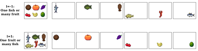
b)

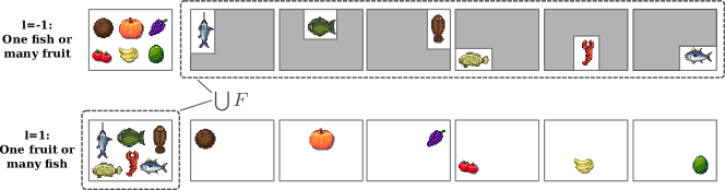
Figure 10: Illustration of a data space with strong asymmetric feature correlation. a): A dataset with fish and fruit features. The features are asymmetrically correlated, because all the fruit features are maximally correlated in class $-1$ (they are all in the same image) and maximally uncorrelated in $1$ (no two fruits share the same image). The reverse is true for the fruits. See Figure 11 for a strategy for Merlin that ensures strong completeness and soundness with uninformative features.
b): Asymmetric feature correlation for a specific feature selection. For the class $-1$, we select the set $F$ of all “fish” features. Each individual fish feature in $F$ covers a fraction of $\frac{1}{6}$ of $(F^{\ast})\cap D_{-1}$ and all images (one) in $(F^{\ast})\cap D_{1}$. The expected value in Equation 6 thus evaluates to $k=6$. This is also the maximum AFC for the entire dataset as no different feature selection gives a higher value.

For an illustration of the asymmetric feature correlation, consider two-class data space $\mathfrak{D}=\mathopen{}\left\{D,\mathcal{D},c\right\}\mathclose{}$, e.g. the “fish and fruit” data depicted in Figure 10. Let us choose $F\subset D_{p}$ to be all the “fish” features. We see that these features are strongly anti-concentrated in class $l=-1$ (none of them share an image) and strongly concentrated in class $l=1$ (all of them are in the same image).

For now, let us assume $F$ is finite and let $\mathcal{F}=\mathcal{U}(F)$, the uniform measure over $F$. We have strong AFC if the class-wise ratio of what each feature covers individually is much larger than what the features cover as a whole:

$$\mathbb{E}_{\mathbf{z}\sim\mathcal{F}}\mathopen{}\left[\frac{\mathbb{P}_{\mathbf{x}\sim\mathcal{D}_{-l}}\mathopen{}\left[\mathbf{z}\subseteq\mathbf{x}\right]\mathclose{}}{\mathbb{P}_{\mathbf{x}\sim\mathcal{D}_{l}}\mathopen{}\left[\mathbf{z}\subseteq\mathbf{x}\right]\mathclose{}}\right]\mathclose{}\gg\frac{\mathbb{P}_{\mathbf{x}\sim\mathcal{D}_{-l}}\mathopen{}\left[\mathbf{x}\in F^{\ast}\right]\mathclose{}}{\mathbb{P}_{\mathbf{x}\sim\mathcal{D}_{l}}\mathopen{}\left[\mathbf{x}\in F^{\ast}\right]\mathclose{}}.$$

In our example, every individual “fish” feature covers one image in each class, so the left side is equal to 1. As a feature set, they cover 6 images in class $-1$ and one in class $1$, so the right side is $\frac{1}{6}$. Using

$$\frac{\mathbb{P}\mathopen{}\left[\mathbf{z}\subseteq\mathbf{x}\right]\mathclose{}}{\mathbb{P}\mathopen{}\left[\mathbf{x}\in F^{\ast}\right]\mathclose{}}=\mathbb{P}\mathopen{}\left[\mathbf{z}\subseteq\mathbf{x}\,|\,\mathbf{x}\in F^{\ast}\right]\mathclose{},$$

we can restate this expression as

$$\mathbb{E}_{\mathbf{z}\sim\mathcal{F}}\mathopen{}\left[\kappa_{l}(\mathbf{z},F)\right]\mathclose{}\gg 1,$$ (6)

where

$$\kappa_{l}(\mathbf{z},F)=\frac{\mathbb{P}_{\mathbf{x}\sim\mathcal{D}_{-l}}\mathopen{}\left[\mathbf{z}\subseteq\mathbf{x}\,|\,\mathbf{x}\in F^{\ast}\right]\mathclose{}}{\mathbb{P}_{\mathbf{x}\sim\mathcal{D}_{l}}\mathopen{}\left[\mathbf{z}\subseteq\mathbf{x}\,|\,\mathbf{x}\in F^{\ast}\right]\mathclose{}}.$$

For our “fish” features we have $\kappa_{-1}(\mathbf{z},F)=6$ for every feature $\mathbf{z}\in F$. Considering an infinite set $F$, we need a way to get a reasonable measure $\mathcal{F}$, where we don’t want to “overemphasise” features that appear only in very few data points. We thus define a feature selector $f_{F}\in\mathcal{M}(F^{\ast})$ as

$$f_{F}(\mathbf{x})=\operatorname*{arg\,max}_{\begin{subarray}{c}\mathbf{z}\in F\\ \text{s.t. }\mathbf{z}\subseteq\mathbf{x}\end{subarray}}\kappa(\mathbf{z},F),$$ (7)

and we can define the push-forward measure $\mathcal{F}=f_{F*}\mathcal{D}_{l}|_{F^{\ast}}$. For our fish and fruit example, where $F$ is the set of all fish features, $f_{F*}$ would select a fish feature for every image in class $-1$ that is in $F^{\ast}$. Putting everything together, we get the following definition.

Definition B.1 (Asymmetric feature correlation).

Let $(D,\mathcal{D},c)$ be a two-class data space, then the asymmetric feature correlation $\kappa$ is defined as

$$\kappa=\max_{l\in\mathopen{}\left\{-1,1\right\}\mathclose{}}\max_{F\subset D_{p}}\,\mathbb{E}_{\mathbf{y}\sim\mathcal{D}_{l}|_{F^{\ast}}}\mathopen{}\left[\max_{\begin{subarray}{c}\mathbf{z}\in F\\ \text{s.t. }\mathbf{z}\subseteq\mathbf{y}\end{subarray}}\frac{\mathbb{P}_{\mathbf{x}\sim\mathcal{D}_{-l}}\mathopen{}\left[\mathbf{z}\subseteq\mathbf{x}\,\middle|\,\mathbf{x}\in F^{\ast}\right]\mathclose{}}{\mathbb{P}_{\mathbf{x}\sim\mathcal{D}_{l}}\mathopen{}\left[\mathbf{z}\subseteq\mathbf{x}\,\middle|\,\mathbf{x}\in F^{\ast}\right]\mathclose{}}\right]\mathclose{}.$$

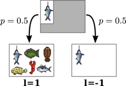
Figure 11: In the dataset presented in Figure 10, Merlin can use the strategy to always select the fish features for class $l=-1$ and the fruit features for class $l=1$ if they exist and choose something arbitrary otherwise. Arthur can then guess $l=1$ if he gets a fish and $l=-1$ for a fruit. This strategy fails only for the images containing all fruits or fish, and can only be exploited by Morgana for those same two images out of 14. The completeness and soundness constants in this case are both $\frac{1}{7}$. But as illustrated here, each “fish” feature is completely uninformative of the class. Conditioned on the selected fish, it could either be the image from class $l=-1$ or from $l=1$.

As we have seen in the “fish and fruit” example, the AFC can be made arbitrarily large, as long as one can fit many individual features into a single image. We can prove that the maximum amount of features per data point indeed also gives an upper bound on the AFC. We now come back to 2.10 and prove it. See 2.10

Proof.

Let $l\in\mathopen{}\left\{-1,1\right\}\mathclose{}$ and let $F\subset D_{p}$. We define $f_{F}\in\mathcal{M}(F^{\ast})$ as in Equation 7 as well as $\mathcal{F}=f_{F*}\mathcal{D}_{l}|_{F^{\ast}}$. We can assert that

$$\mathbb{P}_{\mathbf{x}\sim\mathcal{D}_{l}}\mathopen{}\left[\mathbf{z}\subseteq\mathbf{x}\,|\,\mathbf{x}\in F^{\ast}\right]\mathclose{}\geq\mathbb{P}_{\mathbf{x}\sim\mathcal{D}_{l}}\mathopen{}\left[f(\mathbf{x})=\mathbf{z}\,|\,\mathbf{x}\in F^{\ast}\right]\mathclose{}=\mathcal{F}(\mathbf{z}).$$ (8)

We then switch the order of taking the expectation value in the definition of the AFC:

$$\kappa_{l}(F) =\mathbb{E}_{\mathbf{z}\sim\mathcal{F}}\mathopen{}\left[\frac{\mathbb{P}_{\mathbf{x}\sim\mathcal{D}_{-l}}\mathopen{}\left[\mathbf{x}\in F\,|\,\mathbf{x}\in F^{\ast}\right]\mathclose{}}{\mathbb{P}_{\mathbf{y}\sim\mathcal{D}_{l}}\mathopen{}\left[\mathbf{z}\subseteq\mathbf{y}\,|\,\mathbf{y}\in F^{\ast}\right]\mathclose{}}\right]\mathclose{}$$

$$=\mathbb{E}_{\mathbf{z}\sim\mathcal{F}}\mathopen{}\left[\frac{\mathbb{E}_{\mathbf{x}\sim\mathcal{D}_{-l}}\mathopen{}\left[\mathbbm{1}\mathopen{}\left(\mathbf{z}\subseteq\mathbf{x}\right)\mathclose{}\,|\,\mathbf{x}\in F^{\ast}\right]\mathclose{}}{\mathbb{P}_{\mathbf{y}\sim\mathcal{D}_{l}}\mathopen{}\left[\mathbf{z}\subseteq\mathbf{y}\,|\,\mathbf{y}\in F^{\ast}\right]\mathclose{}}\right]\mathclose{}$$

$$=\mathbb{E}_{\mathbf{x}\sim\mathcal{D}_{-l}}\mathopen{}\left[\mathbb{E}_{\mathbf{z}\sim\mathcal{F}}\mathopen{}\left[\frac{\mathbbm{1}\mathopen{}\left(\mathbf{z}\subseteq\mathbf{x}\right)\mathclose{}}{\mathbb{P}_{\mathbf{y}\sim\mathcal{D}_{l}}\mathopen{}\left[\mathbf{z}\subseteq\mathbf{y}\,|\,\mathbf{y}\in F^{\ast}\right]\mathclose{}}\right]\mathclose{}\,\middle|\,\mathbf{x}\in F^{\ast}\right]\mathclose{}.$$

Since there are only finitely many features in a data point we can express the expectation value over a countable sum weighted by the probability of each feature:

$$\kappa_{l}(F) =\mathbb{E}_{\mathbf{x}\sim\mathcal{D}_{-l}}\mathopen{}\left[\sum_{\mathbf{z}\in F:\,\mathbf{x}\in F}\mathopen{}\left[\frac{\mathcal{F}(\mathbf{z})}{\mathbb{P}_{\mathbf{y}\sim\mathcal{D}_{l}}\mathopen{}\left[\mathbf{z}\subseteq\mathbf{y}\,|\,\mathbf{y}\in F^{\ast}\right]\mathclose{}}\right]\mathclose{}\,\middle|\,\mathbf{x}\in F^{\ast}\right]\mathclose{}$$

$$\leq\mathbb{E}_{\mathbf{x}\sim\mathcal{D}_{-l}}\mathopen{}\left[\sum_{\mathbf{z}\in F:\,\mathbf{x}\in F}1\,\middle|\,\mathbf{x}\in F^{\ast}\right]\mathclose{}$$

$$\leq\mathbb{E}_{\mathbf{x}\sim\mathcal{D}_{-l}}\mathopen{}\left[K\,\middle|\,\mathbf{x}\in F^{\ast}\right]\mathclose{}$$

$$=K,$$

where in the first step we used Equation 8 and the definition of $K$ in the second. Then we see that

$$\kappa=\max_{l\in\mathopen{}\left\{-1,1\right\}\mathclose{}}\max_{F\subset D_{p}}~{}\kappa_{l}(F)\leq K.$$

∎

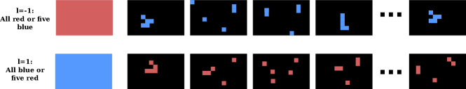
Figure 12: An example of a dataset with very high asymmetric feature correlation. The completely red image shares a feature with each of the $m$-red-pixel images (here $m=5$), of which there are $\binom{d}{m}$ many. In the worst case $m=\frac{d}{2}$, resulting in $k=\binom{d}{d/2}$ thus exponential growth in $d$.

The number of features per data point is dependent on which kinds of features we consider. Without limitations, this number can be $2^{d}$, i.e., exponentially high. See Figure 12 for an example of exponentially large AFC parameters. If we consider only features of a fixed size and shape, such as in image data, the number of features per data point drops to $\approx d$.

We now prove an intermediate lemma that will later allow us to prove 2.12.

Lemma B.2.

Let $(D,\mathcal{D},c)$ be a two-class data space with asymmetric feature correlation of $\kappa$ and class imbalance $B$. Let $A:[0,1]^{d}\rightarrow\mathopen{}\left\{-1,0,1\right\}\mathclose{}$ be a feature classifier and $M\in\mathcal{M}(D)$ a feature selector for $D$. From

1. Completeness:
   

   $$\min_{l\in\mathopen{}\left\{-1,1\right\}\mathclose{}}\mathbb{P}_{\mathbf{x}\sim\mathcal{D}_{l}}\mathopen{}\left[A\mathopen{}\left(M(\mathbf{x})\right)\mathclose{}=l\right]\mathclose{}\geq 1-\epsilon_{c},$$

2. Soundness:
   

   $$\max\limits_{\widehat{M}\in\mathcal{M}(D)}\max\limits_{l\in\mathopen{}\left\{-1,1\right\}\mathclose{}}\mathbb{P}_{\mathbf{x}\sim\mathcal{D}_{l}}\mathopen{}\left[A\mathopen{}\left(\widehat{M}(\mathbf{x})\right)\mathclose{}=-l\right]\mathclose{}\leq\epsilon_{s},$$

follows

$$Q_{\mathcal{D}}(M)\geq 1-\epsilon_{c}-\frac{\kappa\epsilon_{s}}{1-\epsilon_{c}+\kappa\epsilon_{s}B^{-1}}.$$

This lemma gives a bound on the probability that data points with features selected by Merlin will also belong to the same class. This probability is large as long as we have a bound on the AFC of the dataset.

Proof.

The proof of our lemma is fairly intuitive, although the notation can appear cumbersome. Here we give a quick overview over the proof steps.

1. In the definition of the AFC, we maximise over all possible features sets. We will choose as a special case (for each class $l\in\mathopen{}\left\{-1,1\right\}\mathclose{}$) the features that Merlin selects for data points that Arthur classifies correctly.

2. These feature sets cover the origin class at least up to $1-\epsilon_{c}$, and the other class at most up to $\epsilon_{s}$, which is required by the completeness and soundness criteria, respectively. This gives us a high precision for the whole feature set.

3. The AFC upper bounds the quotient of the precision of the whole feature set and expected precision of the individual features, which finally allows us to state our result.

Let us define a partition of $D$ according to the true class and the class assigned by Arthur. From now on, let $l\in\mathopen{}\left\{-1,1\right\}\mathclose{}$ and $m\in\mathopen{}\left\{-1,0,1\right\}\mathclose{}$. We introduce the datasets

$$D_{l,m}=\mathopen{}\left\{\mathbf{x}\in D_{l}\,|\,A(M(\mathbf{x}))=m\right\}\mathclose{},$$

which means that $D_{l,l}$ are the data points that Arthur classifies correctly, and furthermore

$$F_{l}=M(D_{l,l}).$$

To use the AFC bound we need a feature selector $f:D_{l}|_{F^{\ast}}\rightarrow F$. Merlin itself maps to features outside $F$ when applied to data points in $D_{l}|_{F^{\ast}_{l}}\setminus D_{l,l}$. Let us thus define $\sigma:D_{F}\setminus D_{l,l}\rightarrow F$ which selects an arbitrary feature from $F$ (in case one is concerned whether such a representative can always be chosen, consider a discretised version of the data space which allows for an ordering). Then we can define

$$f(\mathbf{x})=\begin{cases}M(\mathbf{x})&\mathbf{x}\in D_{l,l},\\ \sigma(\mathbf{x})&\mathbf{x}\in D_{l}|_{F^{\ast}_{l}}\setminus D_{l,l},\end{cases}\quad\text{and}\quad\mathcal{F}_{l}=f_{\ast}D_{l}|_{F^{\ast}_{l}}.$$

This feature selector will allow us to use the AFC bound. We now abbreviate

$$p(\mathbf{x},f)=\mathbb{P}_{\mathbf{y}\sim\mathcal{D}}\mathopen{}\left[c(\mathbf{y})\neq c(\mathbf{x})\,|\,\mathbf{y}\in f(\mathbf{x})\right]\mathclose{}\quad\text{and}\quad P_{l}=\mathbb{P}_{\mathbf{x}\sim\mathcal{D}}\mathopen{}\left[\mathbf{x}\in D_{l}\right]\mathclose{}.$$

Then

$$1-Q_{\mathcal{D}}(M)=\mathbb{E}_{\mathbf{x}\sim\mathcal{D}}\mathopen{}\left[p(\mathbf{x},M)\right]\mathclose{}=\sum_{l\in\mathopen{}\left\{-1,1\right\}\mathclose{}}\mathbb{E}_{\mathbf{x}\sim\mathcal{D}_{l}}\mathopen{}\left[p(\mathbf{x},M)\right]\mathclose{}P_{l}.$$ (9)

Using the completeness criterion and the fact that $p(\mathbf{x},M)\leq 1$ we can bound

$$\mathbb{E}_{\mathbf{x}\sim\mathcal{D}_{l}}\mathopen{}\left[p(\mathbf{x},M)\right]\mathclose{} =\mathbb{E}_{\mathbf{x}\sim\mathcal{D}_{l}}\mathopen{}\left[p(\mathbf{x},M)\mathbbm{1}\mathopen{}\left(\mathbf{x}\in D_{l,l}\right)\mathclose{}\right]\mathclose{}+\mathbb{E}_{\mathbf{x}\sim\mathcal{D}_{l}}\mathopen{}\left[p(\mathbf{x},M)\mathbbm{1}\mathopen{}\left(\mathbf{x}\notin D_{l,l}\right)\mathclose{}\right]\mathclose{}$$

$$\leq\mathbb{E}_{\mathbf{x}\sim\mathcal{D}_{l}}\mathopen{}\left[p(\mathbf{x},M)\mathbbm{1}\mathopen{}\left(\mathbf{x}\in D_{l,l}\right)\mathclose{}\right]\mathclose{}+\epsilon_{c}$$

$$\leq\mathbb{E}_{\mathbf{x}\sim\mathcal{D}_{l}}\mathopen{}\left[p(\mathbf{x},M)\mathbbm{1}\mathopen{}\left(\mathbf{x}\in D_{l,l}\right)\mathclose{}\right]\mathclose{}+\epsilon_{c}+\mathbb{E}_{\mathbf{x}\sim\mathcal{D}_{l}}\mathopen{}\left[p(\mathbf{x},\sigma)\mathbbm{1}\mathopen{}\left(\mathbf{x}\in D_{l}|_{F^{\ast}_{l}}\setminus D_{l,l}\right)\mathclose{}\right]\mathclose{}$$

$$\leq\frac{\mathbb{E}_{\mathbf{x}\sim\mathcal{D}_{l}}\mathopen{}\left[p(\mathbf{x},M)\mathbbm{1}\mathopen{}\left(\mathbf{x}\in D_{l,l}\right)\mathclose{}+p(\mathbf{x},\sigma)\mathbbm{1}\mathopen{}\left(\mathbf{x}\in D_{l}|_{F^{\ast}_{l}}\setminus D_{l,l}\right)\mathclose{}\right]\mathclose{}}{\mathbb{P}_{\mathbf{x}\sim\mathcal{D}_{l}}\mathopen{}\left[\mathbf{x}\in D_{l}|_{F^{\ast}_{l}}\right]\mathclose{}}+\epsilon_{c}$$

$$=\mathbb{E}_{\mathbf{x}\sim\mathcal{D}_{l}|_{F^{\ast}_{l}}}\mathopen{}\left[p(\mathbf{x},f)\right]\mathclose{}+\epsilon_{c}$$

$$=\mathbb{E}_{\mathbf{z}\sim\mathcal{F}_{l}}\mathopen{}\left[\mathbb{P}_{\mathbf{y}\sim\mathcal{D}}\mathopen{}\left[c(\mathbf{y})=-l\,|\,\mathbf{z}\subseteq\mathbf{y}\right]\mathclose{}\right]\mathclose{}+\epsilon_{c}.$$

We can expand the expression in the expectation using Bayes’ Theorem:

$$\mathbb{P}_{\mathbf{y}\sim\mathcal{D}}\mathopen{}\left[c(\mathbf{y})=-l\,|\,\mathbf{y}\in\mathbf{z}\right]\mathclose{} =\frac{\mathbb{P}_{\mathbf{y}\sim\mathcal{D}_{-l}}\mathopen{}\left[\mathbf{z}\subseteq\mathbf{y}\right]\mathclose{}\mathbb{P}_{-l}}{\mathbb{P}_{\mathbf{y}\sim\mathcal{D}_{-l}}\mathopen{}\left[\mathbf{z}\subseteq\mathbf{y}\right]\mathclose{}P_{-l}+\mathbb{P}_{\mathbf{y}\sim\mathcal{D}_{l}}\mathopen{}\left[\mathbf{z}\subseteq\mathbf{y}\right]\mathclose{}P_{l}}$$

$$=h\mathopen{}\left(\frac{\mathbb{P}_{\mathbf{y}\sim\mathcal{D}_{-l}}\mathopen{}\left[\mathbf{z}\subseteq\mathbf{y}\right]\mathclose{}\mathbb{P}_{-l}}{\mathbb{P}_{\mathbf{y}\sim\mathcal{D}_{l}}\mathopen{}\left[\mathbf{z}\subseteq\mathbf{y}\right]\mathclose{}P_{l}}\right)\mathclose{},$$

where $h(t)=(1+t^{-1})^{-1}$. Since $h(t)$ is a concave function for $t\geq 0$, we know that for any random variable $R$ have $\mathbb{E}\mathopen{}\left[h(R)\right]\mathclose{}\leq h(\mathbb{E}\mathopen{}\left[R\right]\mathclose{})$, so

$$\mathbb{E}_{\mathbf{x}\sim\mathcal{D}_{l}}\mathopen{}\left[p(\mathbf{x},M)\right]\mathclose{}\leq h\mathopen{}\left(\mathbb{E}_{\mathbf{z}\sim\mathcal{F}_{l}}\mathopen{}\left[\frac{\mathbb{P}_{\mathbf{y}\sim\mathcal{D}_{-l}}\mathopen{}\left[\mathbf{z}\subseteq\mathbf{y}\right]\mathclose{}}{\mathbb{P}_{\mathbf{y}\sim\mathcal{D}_{l}}\mathopen{}\left[\mathbf{z}\subseteq\mathbf{y}\right]\mathclose{}}\right]\mathclose{}\frac{P_{-l}}{P_{l}}\right)\mathclose{}+\epsilon_{c}.$$ (10)

From the definition of the AFC $\kappa$ we know that

$$\mathbb{E}_{\mathbf{z}\sim\mathcal{F}_{l}}\mathopen{}\left[\frac{\mathbb{P}_{\mathbf{y}\sim\mathcal{D}_{-l}}\mathopen{}\left[\mathbf{z}\subseteq\mathbf{y}\right]\mathclose{}}{\mathbb{P}_{\mathbf{y}\sim\mathcal{D}_{l}}\mathopen{}\left[\mathbf{z}\subseteq\mathbf{y}\right]\mathclose{}}\right]\mathclose{}\leq\mathbb{E}_{\mathbf{x}\sim\mathcal{D}_{l}|_{F^{\ast}_{l}}}\mathopen{}\left[\max_{\begin{subarray}{c}\mathbf{z}\in F\\ \text{s.t. }\mathbf{z}\subseteq\mathbf{x}\end{subarray}}\frac{\mathbb{P}_{\mathbf{y}\sim\mathcal{D}_{-l}}\mathopen{}\left[\mathbf{z}\subseteq\mathbf{y}\right]\mathclose{}}{\mathbb{P}_{\mathbf{y}\sim\mathcal{D}_{l}}\mathopen{}\left[\mathbf{z}\subseteq\mathbf{y}\right]\mathclose{}}\right]\mathclose{}\leq\kappa\frac{\mathbb{P}_{\mathbf{y}\sim\mathcal{D}_{-l}}\mathopen{}\left[\mathbf{y}\in F^{\ast}\right]\mathclose{}}{\mathbb{P}_{\mathbf{y}\sim\mathcal{D}_{l}}\mathopen{}\left[\mathbf{y}\in F^{\ast}\right]\mathclose{}}.$$ (11)

Now we make use of the fact that we can lower bound $\mathbb{P}_{\mathbf{y}\sim\mathcal{D}_{l}}\mathopen{}\left[\mathbf{y}\in F\right]\mathclose{}$ by the completeness property

$$\mathbb{P}_{\mathbf{y}\sim\mathcal{D}_{l}}\mathopen{}\left[\mathbf{y}\in F^{\ast}\right]\mathclose{}\geq 1-\epsilon_{c},$$

and upper bound $\mathbb{P}_{\mathbf{y}\sim\mathcal{D}_{-l}}\mathopen{}\left[\mathbf{y}\in F^{\ast}\right]\mathclose{}$ with the soundness property

$$\mathbb{P}_{\mathbf{y}\sim\mathcal{D}_{-l}}\mathopen{}\left[\mathbf{y}\in F^{\ast}\right]\mathclose{}\leq\epsilon_{s}.$$

This is because $\mathbf{y}\in F^{\ast}$ implies that there are features Morgana can use to convince Arthur of class $l$ whereas $\mathbf{y}\sim\mathcal{D}_{-l}$. Together with Equation 10 and Equation 11 we arrive at

$$\mathbb{E}_{\mathbf{x}\sim\mathcal{D}_{l}}\mathopen{}\left[p(\mathbf{x},M)\right]\mathclose{}\leq h\mathopen{}\left(\kappa\frac{\epsilon_{s}}{1-\epsilon_{c}}\frac{P_{-l}}{P_{l}}\right)\mathclose{}+\epsilon_{c}=\frac{\kappa\epsilon_{s}\frac{P_{-l}}{P_{l}}}{1-\epsilon_{c}+\kappa\epsilon_{s}\frac{P_{-l}}{P_{l}}}+\epsilon_{c}.$$

Using $\frac{P_{l}}{P_{-l}}\leq B$ thus $\frac{P_{-l}}{P_{l}}\geq B^{-1}$, we can express

$$\mathbb{E}_{\mathbf{x}\sim\mathcal{D}_{l}}\mathopen{}\left[p(\mathbf{x},M)\right]\mathclose{}\leq\frac{\kappa\epsilon_{s}\frac{P_{-l}}{P_{l}}}{1-\epsilon_{c}+\kappa\epsilon_{s}B^{-1}}+\epsilon_{c}.$$

Inserted back into equation Equation 9 leads us to

$$1-Q_{\mathcal{D}}(M)\leq\frac{\kappa\epsilon_{s}}{1-\epsilon_{c}+\kappa\epsilon_{s}B^{-1}}+\epsilon_{c}.$$

∎

B.4 Relative Success Rate and Realistic Algorithms

As discussed in Section 2.4 realistic algorithms will not be optimal players as in 2.8. It will turn out that that we can relax the requirement for Morgana to play optimally in two important ways: (i) She is only required to find features that can also be found by Merlin (2) She only needs success on a similar rate as Merlin. It is thus rather the relative strength between the algorithms used for Merlin and Morgana that is important. We can define relative success rate in the following way:

Definition B.3 (Relative Success Rate).

Let $\mathfrak{D}=(D,\mathcal{D},c)$ be a two-class data space. Let $A\in\mathcal{A}$ and $M,\widehat{M}\in\mathcal{M}(D)$ Then the relative success rate $\alpha$ of $\widehat{M}$ with respect to $A,M$ and $\mathfrak{D}$ is defined as

$$\alpha:=\min_{l\in\mathopen{}\left\{-1,1\right\}\mathclose{}}\frac{\mathbb{P}_{\mathbf{x}\sim\mathcal{D}_{-l}}\mathopen{}\left[A(\widehat{M}(\mathbf{x}))=l\,|\,\mathbf{x}\in F_{l}^{\ast}\right]\mathclose{}}{\mathbb{P}_{\mathbf{x}\sim\mathcal{D}_{l}}\mathopen{}\left[A(M(\mathbf{x}))=l\,|\,\mathbf{x}\in F_{l}^{\ast}\right]\mathclose{}}.\quad\text{where}\quad F_{l}:=\mathopen{}\left\{\mathbf{z}\in D_{p}\,|\,\mathbf{z}\in M(D_{l}),A(\mathbf{z})=l\right\}\mathclose{}.$$

The set $F_{l}$ contains all features that Merlin selects in class $l$ that successfully convince Arthur of class $l$. We condition on the fact that a feature that Merlin uses is in the datapoint and then compare the rates of Morgana and Merlin convincing Arthur. Morgana can of course also select different features but is not required to find features that also Merlin could not find.

Given that one of Merlins features is in the datapoint, the question is thus how much the context given by the other features affect the hardness of finding of the former. We can easily construct scenarios in which the context matters very strongly, see Figure 13 for an example. We expect that for most real-world data this dependence is only weak and can be upper bounded.

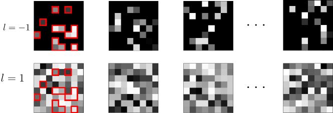
Figure 13: Illustration of a dataset with strong context dependence. Class $-1$ consists of $k$-sparse images whose pixel values sum to some number $S$. For each of these images, there is a non-sparse image in class $1$ that shares all non-zero values (marked in red for the first image). Merlin can use the strategy to show all $k$ non-zero pixels for an image from class $-1$ and $k+1$ arbitrary non-zero pixels for class $1$. Arthur checks if the sum is equal to $S$ or if the number of pixels equal to $k+1$, otherwise he says “I don’t know!”. He will then classify with 100% accuracy. Nevertheless, the features Merlin uses for class $-1$ are completely uncorrelated with the class label. To exploit this, however, Morgana would have to solve the $\mathsf{NP}$-hard (Kleinberg & Tardos, 2006) subset sum problem to find the pixels for images in class 1 that sum to $S$. The question is not in which class we can find the features, but in which class we can find the features efficiently.

Example B.4.

Let $\mathfrak{D}$ be a data space with maximum number of features per data point $K$. Let Morgana operate the algorithm described in Algorithm 1, in which she randomly searches for a convincing feature. Then we have

$$\alpha\geq\frac{K}{n_{\text{try}}},$$

which corresponds to an upper bound on the probability that Morgana will succeed on an individual data point when there is only one convincing feature.

1:  Input: $\mathbf{x}\in D$, $n_{\text{try}}$

2:  Output: $\mathbf{z}\in D_{p}$

3:  for $i\in[n_{\text{try}}]$ do

4:     Pick random feature $\mathbf{z}$ s.t. $\mathbf{z}\in\mathbf{x}$

5:     if $A(\mathbf{z})=-c(\mathbf{x})$ then

6:        return $\mathbf{z}$

7:     end if

8:  end for

9:  return $\varnothing$

Algorithm 1 Merlin-Arthur Training

We generally want Morgana’s algorithm to be at least as powerful as Merlin’s so in case of an optimiser one can consider giving more iterations or more initial starting values.

We now want to prove 2.12 which we restate here.

See 2.12

Proof.

We follow the same proof steps and definitions as in the proof of B.2 up to Equation 11. Then we consider the following

$$\alpha\frac{\mathbb{P}_{\mathbf{y}\sim\mathcal{D}_{-l}}\mathopen{}\left[\mathbf{y}\in F\right]\mathclose{}}{\mathbb{P}_{\mathbf{y}\sim\mathcal{D}_{l}}\mathopen{}\left[\mathbf{y}\in F\right]\mathclose{}} \leq\frac{\mathbb{P}_{\mathbf{y}\sim\mathcal{D}_{-l}}\mathopen{}\left[\mathbf{y}\in F\right]\mathclose{}}{\mathbb{P}_{\mathbf{y}\sim\mathcal{D}_{l}}\mathopen{}\left[\mathbf{y}\in F\right]\mathclose{}}\frac{\mathbb{P}_{\mathbf{x}\sim\mathcal{D}_{-l}}\mathopen{}\left[A(\widehat{M}(\mathbf{x}))=l\,|\,\mathbf{x}\in F_{l}^{\ast}\right]\mathclose{}}{\mathbb{P}_{\mathbf{x}\sim\mathcal{D}_{l}}\mathopen{}\left[A(M(\mathbf{x}))=l\,|\,\mathbf{x}\in F_{l}^{\ast}\right]\mathclose{}}$$ (12)

$$=\frac{\mathbb{P}_{\mathbf{x}\sim\mathcal{D}_{-l}}\mathopen{}\left[A(\widehat{M}(\mathbf{x}))=l,\,\mathbf{x}\in F_{l}^{\ast}\right]\mathclose{}}{\mathbb{P}_{\mathbf{x}\sim\mathcal{D}_{l}}\mathopen{}\left[A(M(\mathbf{x}))=l,\,\mathbf{x}\in F_{l}^{\ast}\right]\mathclose{}}$$ (13)

$$\leq\frac{\mathbb{P}_{\mathbf{x}\sim\mathcal{D}_{-l}}\mathopen{}\left[A(\widehat{M}(\mathbf{x}))=l\right]\mathclose{}}{\mathbb{P}_{\mathbf{x}\sim\mathcal{D}_{l}}\mathopen{}\left[A(M(\mathbf{x}))=l\right]\mathclose{}}$$ (14)

where in the last step we used that $\mathbf{x}\in D_{l}\wedge A(M(\mathbf{x}))=l\,\Rightarrow\,\mathbf{x}\in F_{l}^{\ast}$ by definition of $F_{l}^{\ast}$. We know by the soundness and completeness criteria that

$$\mathbb{P}_{\mathbf{x}\sim\mathcal{D}_{-l}}\mathopen{}\left[A(M(\mathbf{x},l))=l\right]\mathclose{}\leq\epsilon_{s}\quad\text{and}\quad\mathbb{P}_{\mathbf{x}\sim\mathcal{D}_{l}}\mathopen{}\left[M(\mathbf{x},l)\in F\right]\mathclose{}\geq 1-\epsilon_{c}$$

Putting everything together we arrive at

$$\frac{\mathbb{P}_{\mathbf{y}\sim\mathcal{D}_{-l}}\mathopen{}\left[\mathbf{y}\in F\right]\mathclose{}}{\mathbb{P}_{\mathbf{y}\sim\mathcal{D}_{l}}\mathopen{}\left[\mathbf{y}\in F\right]\mathclose{}}\leq\frac{\alpha^{-1}\epsilon_{s}}{1-\epsilon_{c}},$$

which allows us to continue the proof analogously to B.2. ∎

B.5 Finite and Biased datasets

Real datasets come with further challenges when evaluating the completeness and soundness.

Let us introduce two data distributions $\mathcal{T}$ and $\mathcal{D}$ on the same dataset $D$, where $\mathcal{T}$ is considered the “true” distribution and $\mathcal{D}$ a different, potentially biased, distribution. We define this bias with respect to a specific feature $\mathbf{z}\in D_{p}$ as

$$d^{l}_{\mathbf{z}}(\mathcal{D},\mathcal{T}):=\mathopen{}\left|\mathbb{P}_{\mathbf{x}\in\mathcal{D}}\mathopen{}\left[c(\mathbf{x})=l\,|\,\mathbf{z}\in\mathbf{x}\right]\mathclose{}-\mathbb{P}_{\mathbf{x}\in\mathcal{T}}\mathopen{}\left[c(\mathbf{x})=l\,|\,\mathbf{z}\in\mathbf{x}\right]\mathclose{}\right|\mathclose{}.$$

Note that $d^{1}_{\mathbf{z}}(\mathcal{D},\mathcal{T})=d^{-1}_{\mathbf{z}}(\mathcal{D},\mathcal{T})=\colon d_{\mathbf{z}}(\mathcal{D},\mathcal{T})$ and $0\leq d_{\mathbf{z}}(\mathcal{D},\mathcal{T})\leq 1$. This distance measures if data points containing $\mathbf{z}$ are distributed differently to the two classes for the two distributions.

For example, consider as $\mathbf{z}$ the water in the boat images of the PASCAL VOC dataset Lapuschkin et al. (2019). The feature is a strong predictor for the “boat” class in the test data distribution $\mathcal{D}$ but should not be indicative for the real world distribution which includes images of water without boats and vice versa. We now want to prove that a feature selected by $M$ is either an informative feature or is misrepresented in the test dataset.

Lemma B.5.

Let $\mathfrak{D},k,B,A,M,\alpha,\epsilon_{c}$ and $\epsilon_{s}$ be defined as in 2.12. Let $\mathcal{T}$ be the true data distribution on $D$. Then for $\delta\in[0,1]$ we have

$$\mathbb{P}_{\mathbf{y}\sim\mathcal{T}}\mathopen{}\left[c(\mathbf{y})=c(\mathbf{x})\,|\,M(\mathbf{x})\subseteq\mathbf{y}\right]\mathclose{}\geq 1-\delta-d_{M(\mathbf{x})}(\mathcal{D},\mathcal{T}),$$

with probability $1-\frac{1}{\delta}\mathopen{}\left(\frac{k\alpha\epsilon_{s}}{1+k\alpha\epsilon_{s}B^{-1}-\epsilon_{c}}+\epsilon_{c}\right)\mathclose{}$ for $\mathbf{x}\sim\mathcal{D}$.

This follows directly from 2.7, 2.12, the definition of $d_{\mathbf{z}}(\mathcal{D},\mathcal{T})$ and the triangle inequality. This means that if an unintuitive feature was selected in the test dataset, we can pinpoint to where the dataset might be biased.

We provided B.5 in the context of biased datasets. The next iteration considers the fact that we only sample a finite amount of data from the possibly biased test data distribution. This will only give us an approximate idea of the soundness and completeness constants.

Lemma B.6.

Let $D,\sigma,\mathcal{D},cA,M$ and $\mathcal{T}$ be defined as in B.5. Let $D^{\text{test}}=\mathopen{}\left(\mathbf{x}_{i}\right)\mathclose{}_{i=1}^{N}\sim\mathcal{D}^{N}$ be $N$ random samples from $\mathcal{D}$. Let

$$\epsilon^{\text{test}}_{c}=\max_{l\in\mathopen{}\left\{-1,1\right\}\mathclose{}}\frac{1}{N}\sum_{\mathbf{x}\in D^{\text{test}}_{l}}\mathbbm{1}(A\mathopen{}\left(M(\mathbf{x},c(\mathbf{x}))\right)\mathclose{}\neq c(\mathbf{x})),$$

and

$$\epsilon^{\text{test}}_{s}=\max_{l\in\mathopen{}\left\{-1,1\right\}\mathclose{}}\frac{1}{N}\sum_{\mathbf{x}\in D^{\text{test}}_{l}}\mathbbm{1}(A\mathopen{}\left(M(\mathbf{x},-c(\mathbf{x}))\right)\mathclose{}=-c(\mathbf{x})).$$

Then it holds with probability $1-\eta$ where $\eta\in[0,1]$ that on the true data distribution $\mathcal{T}$ $A$ and $M$ obey completeness and soundness criteria with

$$\epsilon_{c} \leq\epsilon^{\text{test}}_{c}+\epsilon_{\text{dist}}+\epsilon_{\text{sample}}\quad\text{and}$$

$$\epsilon_{s} \leq\epsilon^{\text{test}}_{s}+\epsilon_{\text{dist}}+\epsilon_{\text{sample}}$$

respectively, where $\epsilon_{\text{dist}}=\max\limits_{l\in\mathopen{}\left\{-1,1\right\}\mathclose{}}\mathopen{}\left\|\mathcal{D}_{l}-\mathcal{T}_{l}\right\|\mathclose{}_{TV}$ and $\epsilon_{\text{sample}}=\sqrt{\frac{1}{2N}\log\mathopen{}\left(\frac{4}{\eta}\right)\mathclose{}}$.

The proof follows trivially from Hoeffding’s inequality and the definition of the total variation norm.

Proof.

We define $E_{c,l}=\mathopen{}\left\{\mathbf{x}\in D_{l}\,|\,A\mathopen{}\left(M(\mathbf{x},c(\mathbf{x}))\right)\mathclose{}\neq c(\mathbf{x})\right\}\mathclose{}$ for $l\in\mathopen{}\left\{-1,1\right\}\mathclose{}$ and let $E^{\mathcal{D}}_{c,l}$ be the Bernoulli random variable for the event that $X\in E_{c,l}$ where $X\sim\mathcal{D}$. Then

$$\mathbb{P}_{\mathbf{x}\sim\mathcal{D}_{l}}\mathopen{}\left[A\mathopen{}\left(M(\mathbf{x},c(\mathbf{x}))\right)\mathclose{}\neq c(\mathbf{x})\right]\mathclose{}=\mathbb{E}\mathopen{}\left[E^{\mathcal{D}}_{c,l}\right]\mathclose{}$$

Using Hoeffding’s inequality we can bound for any $t>0$

$$\mathbb{P}\mathopen{}\left[\mathopen{}\left|\mathopen{}\left(\frac{1}{N}\sum_{\mathbf{x}\in D^{\text{test}}_{l}}\mathbbm{1}(\mathbf{x}\in E_{c,l})\right)\mathclose{}-\mathbb{E}\mathopen{}\left[E^{\mathcal{D}}_{c,l}\right]\mathclose{}\right|\mathclose{}>t\right]\mathclose{}\leq e^{-2nt^{2}}.$$

We choose $t$ such that $e^{-2t^{2}}=\frac{\eta}{4}$. We use a union bound for the maximum over $l\in\mathopen{}\left\{-1,1\right\}\mathclose{}$ which results in a probability of $2\frac{\eta}{4}=\frac{\eta}{2}$ we have

$$\max_{l\in\mathopen{}\left\{-1,1\right\}\mathclose{}}\mathbb{E}\mathopen{}\left[E^{\mathcal{D}}_{c,l}\right]\mathclose{}>\epsilon^{\text{test}}_{c}+\sqrt{\frac{1}{2N}\log\mathopen{}\left(\frac{4}{\eta}\right)\mathclose{}},$$

and thus with $1-\frac{\eta}{2}$ we have $\max_{l\in\mathopen{}\left\{-1,1\right\}\mathclose{}}\mathbb{E}\mathopen{}\left[E^{\mathcal{D}}_{c,l}\right]\mathclose{}\leq\epsilon^{\text{test}}_{c}+\epsilon^{\text{sample}}$. Using the definition of the total variation norm

$$\mathopen{}\left\|\mathcal{T}-\mathcal{D}\right\|\mathclose{}_{TV}=\sup_{J\subset D}\mathopen{}\left|\mathcal{T}(J)-\mathcal{D}(J)\right|\mathclose{},$$

with $J=E_{c,l}$ we can derive $\mathbb{E}\mathopen{}\left[E^{\mathcal{T}}_{c,l}\right]\mathclose{}\leq\mathbb{E}\mathopen{}\left[E^{\mathcal{T}}_{c,l}\right]\mathclose{}+\mathopen{}\left\|\mathcal{T}-\mathcal{D}\right\|\mathclose{}_{TV}$ and thus

$$\epsilon_{c}\leq\epsilon_{c}^{\text{test}}+\epsilon^{\text{sample}}+\epsilon^{\text{dist}}.$$

We can treat $\epsilon_{s}$ analogously and take a union bound over both the completeness and soundness bounds holding which results in the probability of $1-\eta$. ∎

Appendix C Numerical Experiments

For the numerical experiments, we implement Arthur, Merlin and Morgana in Python 3.8 using PyTorch (BSD-licensed). We perform our experiments on the UCI Census Income dataset and the MNIST dataset, which is licensed under the Creative Commons Attribution-Share Alike 3.0 licence.

C.1 Training Setup for Census Income dataset

In the following, we provide an overview of the experiments performed on the Census Income dataset, including preprocessing steps and training configurations.

Please note that, when predicting income, a class map $c:D\rightarrow\mathopen{}\left\{-1,1\right\}\mathclose{}$ cannot be defined for all datapoints, i.e., there are different incomes for exactly the same input. However, only small fraction of data points (0.6%) have this issue.

Data Preprocessing

The UCI Census Income dataset consists of both continuous and categorical features, 14 features in total. The target class is chosen to be the feature “sex”, which contains the categories “male” and “female”, to indicate a possible case of discrimination. The feature “fnlwgt” is removed from the set of features, since it does not contain any meaningful information. In addition, the features “marital-status” and “relationship” are also removed as they strongly indicate the target class. After removal, 11 features remain for each data point. The continuous features are scaled according to the min-max scaling method. To simplify feature masking, all features are padded to a vector of the same fixed dimension. Continuous features are then repeated along the padding dimension, while categorical features are one-hot encoded to the length of the fixed dimension. Note, that the fixed dimension is determined by the categorical feature with the most categories.

Finally, the train and test datasets are balanced with respect to the target class, resulting in 19564 train samples and 9826 test samples.

Model Description

Arthur is modelled as a NN with a single hidden linear layer of size 50 followed by a ReLU activation function. The output is converted to a probability distribution via the softmax function with three output dimensions, where the third dimension corresponds to the “Don’t know!” option. The resulting NN contains approximately 23k parameters. Merlin and Morgana, on the other hand, are modelled as Frank-Wolfe optimisers, which are discussed in more detail in the overview of the experiments conducted on the MNIST dataset.

Model	Learning Rate	Batch Size	Frank-Wolfe Learning Rate	Epochs
Pre-training Arthur	$10^{-4}$	512	-	$100$
Merlin-Arthur Classifier	$0.5$	512	0.1	$20$

Table 1: Configurations for pre-training Arthur and training the Merlin-Arthur classifiers.

Model Selection

The training and testing of the models is divided into two phases. First, we pre-train Arthur on the preprocessed UCI Census Income dataset without Merlin and Morgana. Second, we use the pre-trained model to perform further training including Merlin and Morgana. For the pre-training of Arthur, our experiments were conducted such that the models’ parameters were saved separately after each epoch. Consequently, for each experiment, we had access to a set of candidate models to choose from for further analysis. To ensure high completeness, we select the pre-trained candidate with the highest accuracy with respect to the test dataset. The selected model then represents the pre-trained classifier for all subsequent experiments involving Merlin and Morgana. Similar to the pre-training process, we also stored the model parameters after each epoch of training with Merlin and Morgana. The results presented in Figure 5 correspond to the models with the highest completeness at a soundness of at least 0.9 among all epochs. The training configurations regarding the pre-training of Arthur and the training of the Merlin-Arthur classifiers can be obtained from Table 1.

1:  Input: dataset: $D_{\text{train}}$, Epochs: $N$, $\gamma$

2:  Output: Classifier Network (A), Optional: Masking Networks Merlin $(M)$ and Morgana $(\widehat{M})$

3:  for $i\in[N]$ do

4:     for $\mathbf{x}_{j},\mathbf{y}_{j}\in D_{\text{train}}$ do

5:        $\mathbf{s}_{M}\leftarrow M(\mathbf{x}_{j},\mathbf{y}_{j}),\mathbf{s}_{\widehat{M}}\leftarrow\widehat{M}(\mathbf{x}_{j},\mathbf{y}_{j})$ {$M$ and $\widehat{M}$ can be the optimiser or the NN}

6:        $A\leftarrow\arg\min_{A}(1-\gamma)L_{M}(A(s_{M}\cdot x_{j}),y_{j})+\gamma L_{\widehat{M}}(A(s_{\widehat{M}}\cdot x_{j}),y_{j})$ {Update classifier using masked images}

7:        $M\leftarrow\arg\min L_{M}(A(M(\mathbf{x}_{j})\cdot x_{j}),y_{j})$ {Update only if $M$ is a NN}

8:        $\widehat{M}\leftarrow\arg\max L_{\widehat{M}}(A(\widehat{M}(\mathbf{x}_{j})\cdot x_{j}),y_{j})$ {Update only if $\widehat{M}$ is a NN}

9:     end for

10:     for $\mathbf{x}_{j},\mathbf{y}_{j}\in D_{\text{train}}$ do

11:        $A\leftarrow\arg\min_{A}L(A(x_{j}),y_{j}))$ {Update classifier using regular images}

12:     end for

13:  end for

Algorithm 2 Merlin-Arthur Training

C.2 Training Setup for MNIST

Here, we give a detailed description of our training setup for MNIST and show the error bars of the numerical results presented in the main part of the paper over 10 different training runs.

Structure of Arthur. Arthur is modelled using a neural network. Specifically, we consider a convolutional NN with a ReLU activation function. For the case of 2 classes, we consider a NN with 2 convolution layers, whereas for the 5 class case we consider 3 convolution layers. The output of the convolution is then passed through 2 linear layers before being used for the output. Table 2 describes the used architecture in detail.

Layer Name	Parameters
Conv2D	I=3, O=32, K=3
ReLU
Conv2D	I=32, O=64, K=3
ReLU
Conv2D	I=64, O=64, K=3
ReLU
MaxPool2d	K=2
Linear	I=7744, O=1024
ReLU
Linear	I=1024, O=128
ReLU
Linear	I=128, O=1

Table 2: Description of the neural network architecture used for the Arthur classifier.

Structure of Merlin and Morgana. Recall that Merlin and Morgana aim to ideally solve

$$M(\mathbf{x})=\operatorname*{arg\,min}_{\mathbf{s}\in B_{k}^{d}}L_{M}(A,\mathbf{x},\mathbf{s})\quad\text{and}\quad\widehat{M}(\mathbf{x})=\operatorname*{arg\,max}_{\mathbf{s}\in B_{k}^{d}}L_{\widehat{M}}(A,\mathbf{x},\mathbf{s}),$$

respectively, where $L_{M}$ and $L_{\widehat{M}}$ are the loss functions defined in Section 3, and $B_{k}^{d}$ is the space of $k$-sparse binary vectors. Thus, Merlin and Morgana take an image as input and produce a mask of the same dimension with $k$ one-entries and zero-entries otherwise. We additionally added a regularisation term in the form of $\lambda\mathopen{}\left\|\mathbf{s}\right\|\mathclose{}_{1}$ to both of the objectives, and set $\lambda=0.25$. We realise the pair Merlin and Morgana in four different ways, which we explain in the following. All of these approaches return a mask $\mathbf{s}\in[0,1]^{d}$ that we then binarise by setting the $k$ largest values to one and the rest to zero.

Frank-Wolfe Optimisers

In the first case, Merlin and Morgana are modelled by an optimiser using the Frank-Wolfe algorithm (Jaggi, 2013). We follow the approach outlined by Macdonald et al. (2022) with the Frank-Wolfe package provided by Pokutta et al. (2020). The optimiser searches over a convex relaxation of $B_{k}^{d}$, i.e.,

$$\mathcal{B}_{k}^{d}=\mathopen{}\left\{\mathbf{v}\in[0,1]^{d}\,\middle|\,\mathopen{}\left\|\mathbf{v}\right\|\mathclose{}_{1}\leq k\right\}\mathclose{},$$

the $k$-sparse polytope with radius $1$ limited to the positive octant. To optimise the objective we use the solver made available at https://github.com/ZIB-IOL/StochasticFrankWolfe with 200 iterations.

UNet Approach

For the second case, we model Merlin and Morgana using NNs, specifically a UNet that has already been used in the XAI domain to create saliency maps, see (Dabkowski & Gal, 2017). We copy the UNet design by Ronneberger et al. (2015) since it achieves good results in image segmentation, a task reasonably similar to ours. We predict mask values between zero and one for each image pixel, and rescale the mask should it lie outside of $\mathcal{B}_{k}^{d}$. The binarisation of the mask is ignored during the backpropagation that trains the UNets and only employed to produce the masks that Arthur is trained on.

Hybrid Approach

In the Hybrid approach, Merlin is modelled by a UNet, whereas Morgana is still modelled by the FW-optimiser. This approach is useful since for a sound Arthur that cannot be fooled, the training of the Morgana UNet becomes difficult and the UNet diverges. It then takes a while of training for the UNet to adapt, should Arthur open himself to possible adversarial masks. The optimiser is applied to each individual image instead and can find possible weaknesses instantly.

Class-Networks

One of the alternatives to Merlin and Morgana that we propose are class-specific UNets. Instead of Merlin and Morgana each being represented by a network, there is a UNet associated with each class that is trained to produce a feature mask that convinces Arthur of its own class for any input image, i.e., for $l\in[C]$ try to solve

$$M_{l}(\mathbf{x})=\operatorname*{arg\,min}_{\mathbf{s}\in B_{k}^{d}}-\log\mathopen{}\left(A(\mathbf{s}\cdot\mathbf{x})_{l}\right)\mathclose{}+\lambda\mathopen{}\left\|\mathbf{s}\right\|\mathclose{}_{1}.$$

Merlin is then implemented as an algorithm to choose the UNet corresponding to the true class, so

$$M(\mathbf{x})=M_{c(\mathbf{x})}(\mathbf{x}).$$

Morgana instead uses for each individual image the output of the UNet that most convinces Arthur of a wrong class (maximises the Morgana-loss), i.e.,

$$M(\mathbf{x})=M_{l}(\mathbf{x})\quad\text{with}\quad l=\operatorname*{arg\,max}_{l\in C\setminus\mathopen{}\left\{c(\mathbf{x})\right\}\mathclose{}}L_{\widehat{M}}(A,\mathbf{x},M_{l}(\mathbf{x})).$$

Ideally, this training setup would be more stable than the normal UNet approach. When Arthur cannot be fooled, the class-UNets still have a reasonable objective in convincing him of the correct class, which hopefully prevents divergence as for the Morgana UNet. Experimentally, however, the class-networks proved to be much less stable than the simple UNet approach, see Figure 15.

We give an overview over the parameters used for the four different approaches in Table 3.

Parameter	Value
Batch Size	128
Baseline Value	0.3
Max FW Iterations	200
FW Momentum	0.9
Regularisation $\lambda$	0.25
Max NN Passes	5
Arthur LR	1e-4
Merlin LR	1e-4
Morgana LR	1e-6

Table 3: Values of various parameters used in training.

Merlin-Arthur Classifier Training

The overall training procedure proceeds as outlined in Algorithm 2. We initially train Arthur directly on the training data. In the optimiser approach, this pre-trained network is used to search for the optimal masks for Merlin and Morgana. In the UNet approach, these masks are directly produced by the UNets. Arthur is then trained on the masked images over the whole dataset. The UNets are then trained on the dataset with a fixed Arthur according to their respective objectives. We cycle through this process for 5 epochs. The learning rate is 1e-4 for the Arthur and Merlin network and 1e-6 for the Morgana and the class-specific networks.

C.3 Purely Cooperative Setup and “Cheating” for MNIST

Here, we discuss the Merlin-Arthur classifier when only Merlin is used with no Morgana. Our results demonstrate that the inclusion of Morgana is necessary for Merlin and Arthur to exchange meaningful features and abstain from “cheating”. For a purely cooperative setup, information about the class $c(\mathbf{x})$ that Arthur infers is dominated by the fact that Merlin chose that feature, rather than the feature itself, i.e., $H(c(\mathbf{x})|M(\mathbf{x})=\mathbf{z})\ll H(c(\mathbf{y})|\mathbf{z}\subseteq\mathbf{y})$. We can upper bound $H(c(\mathbf{x})|M(\mathbf{x})=\mathbf{z})$ through the classification error $P_{e}$ that Arthur and Merlin achieve via Fano’s inequality (Fano, 1961):

$$H(c(\mathbf{x})|M(\mathbf{x})=\mathbf{z})\leq H_{b}(P_{e})+P_{e}\log(\mathopen{}\left|C\right|\mathclose{}-1),$$

where $\mathopen{}\left|C\right|\mathclose{}$ is the number of classes. We can then bound the amount of information that is transferred by the choice of the mask rather than the feature itself as

$$I(c(\mathbf{x});M(\mathbf{x})=\mathbf{z})-I(c(\mathbf{y});\mathbf{z}\subseteq\mathbf{y}) =H(c(\mathbf{y})~{}|~{}\mathbf{z}\subseteq\mathbf{y})-H(c(\mathbf{x})~{}|~{}M(\mathbf{x})=\mathbf{z})$$

$$\geq H(c(\mathbf{y})~{}|~{}\mathbf{z}\subseteq\mathbf{y})-(H_{b}(P_{e})+P_{e}\log(\mathopen{}\left|C\right|\mathclose{}-1)).$$

We define the cooperative information as

$$I_{\text{coop}}:=\max\left(0,H(c(\mathbf{y})~{}|~{}\mathbf{z}\subseteq\mathbf{y})-(H_{b}(P_{e})+P_{e}\log(\mathopen{}\left|C\right|\mathclose{}-1))\right),$$

which lower bounds how much Arthur and Merlin “cheat”. We train Merlin and Arthur on the MNIST dataset and show the results in Figure 14 that in the purely cooperative case $I_{\text{coop}}$ keeps the classification error low despite exchanging uninformative features. Including Morgana on the other hand pushes $I_{\text{coop}}$ to zero even for small masks. In this case Merlin produces highly informative features.

Figure 14 depicts “Cheating” measured by $I_{coop}$ over the MNIST test dataset (restricted to 5 classes) for different setups. In a purely cooperative setup, Arthur and Merlin learn to communicate over uninformative features. Thus, the classification error $P_{e}$ stays low, while the conditional entropy of the class with respect to the feature goes up. When Morgana is present and soundness is high (in our analysis $\epsilon_{s}<0.05$), Arthur and Merlin cannot cheat, the classification error increases for small $k$.

Why is this observation important? Note that the purely cooperative setup could already be seen as interpretable. With Merlin as a network it appears as a version of a self-interpreting network. With Merlin as an optimiser, it is similar to Rate-Distortion Explanations (RDE) (Macdonald et al., 2019). In fact, RDE have been criticised for producing “cheating” masks that artificially create features that were not present in the original image (Wäldchen et al., 2022). We connect this to the lack of robustness with respect to Morgana. Designers of self-interpreting setups need to explain how they circumvent the problem of “cheating” masks.

Figure 15 depicts the results from the main paper in more detail. Specifically, it depicts averages and the standard deviation as error bars for each parameter using samples from 10 different training runs. The results presented here are consistent with those presented in the main body of the paper, except for the class networks. The error bars are large for small mask sizes, but shrink as the mask size increases. The class-network approach is considerably less stable than our other implementations, even though it was conceived as a stabler alternative to the simple network approach. One possibility might be that since each UNet both cooperates with Arthur and wants to fool him, they are more sensitive when Arthur changes his focus between achieving good soundness and completeness. We hope that further research will determine if this realisation can be trained in a stable manner.

compat=1.15

	Merlin: Opt	Merlin: Opt, Morgana: Opt
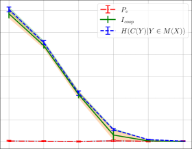
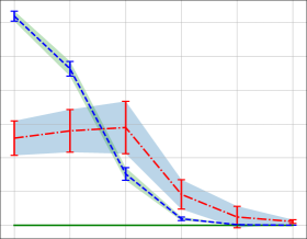
	Merlin: Net	Merlin: Net, Morgana: Opt
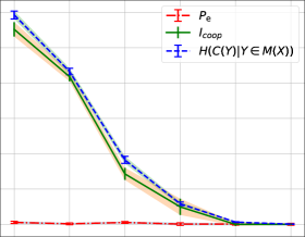
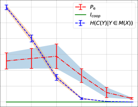
	$k$	$k$

Figure 14: This figure depicts the mean and standard deviation over 10 training runs for the error probability, cooperative information and the class entropy. This was obtained from 5-class classification with classes 1,2,3,4 and 5 with $\gamma=0.75$ for the purely cooperative setup (left) and the adversarial setup (right), where Merlin was realised as an optimiser (top) or as a neural network (bottom).

compat=1.15

	Opt	Hybrid
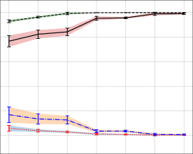
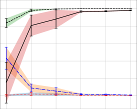
	$k$	$k$
	Net	CN
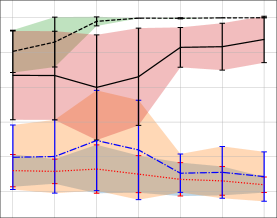
	$k$	$k$

Figure 15: We show the mean and standard deviation over 10 training runs for completeness and soundness, along with the average precision and its bound as obtained from 2-class classification with classes 6 and 9 with $\gamma=0.75$ for different settings.

We also conduct experiments to illustrate the impact of varying values of $\gamma$. The results of these are depicted in Figure 16. As expected, increasing the value of $\gamma$ increases the error rate as it gives more weight to Morgana. This increase is not visible in the NN only setup, indicating this setup may not be creating high quality masks.

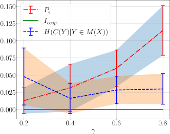
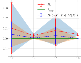
Figure 16: This figure depicts the error probability, cooperative information and the class entropy as obtained from 2-class classification with classes 6 and 9 for different values of $\gamma$ at a mask size of $16$ for the Hybrid (left) and Network (right) settings

C.4 Census income experiments with marital-status and relationship included

In Section 3.1, we demonstrate how an adversarial setup prevents a typical approach to manipulating explanations that has been demonstrated for numerous XAI methods. To show the effect most clearly, we kept the focus on a single sensitive feature (“sex”) and removed the “relationship” and “marital status” features that strongly correlate with it and are thus informative. We now show the results for the experiments including these features in Figure 17, where Merlin uses these features to communicate “sex” with a completeness of 71%.

compat=1.15

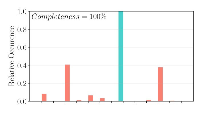
1a) $\beta=0$ $\gamma=0$	1b) $\beta=3.5$ $\gamma=0$
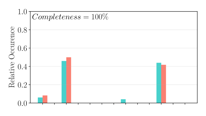
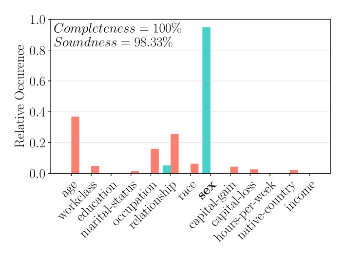
2a) $\beta=3.5$ $\gamma=0.67$	2b) $\beta=10$ $\gamma=0.67$

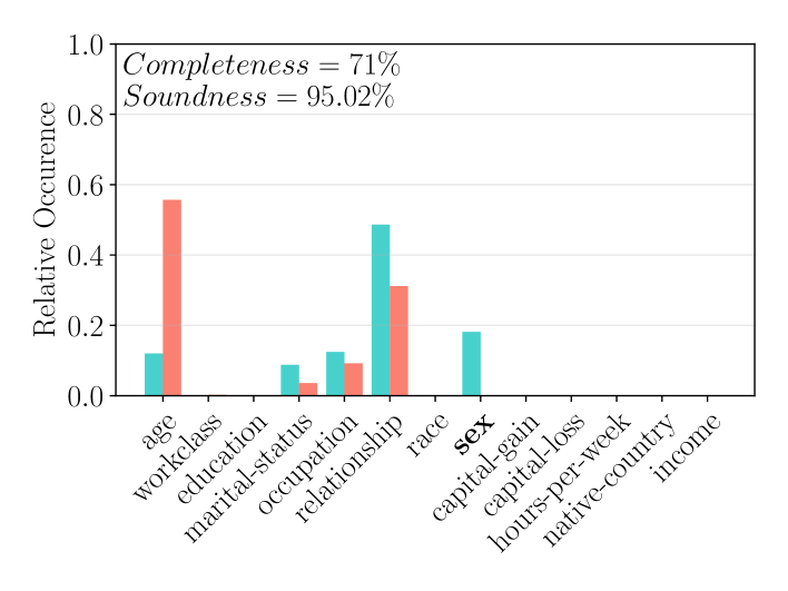
Figure 17: Results from the experiments in Section 3.1, with the features “marital-status” and “relationship” are included. 1) The selected features are the same as in the setup, excluding the two features. 2a) Again, the requirement of soundness results in Merlin selecting “sex” regardless of the punishment. 2b) Despite the higher punishment ($\beta=10$), Arthur and Merlin achieve completeness of 71%, unlike the results presented in Section 3.1, due to the selection of “relationship”, a feature strongly correlated with “sex”.

C.5 Discussion

Our theoretical results are so far only formulated for two classes. We expect them to be extendable to a $n$-class setting, but leave this to further research. It remains to be seen whether our proposed training setup can be extended to more involved datasets while retaining stability. So far, we have kept the training routine straightforward and simple. Similar to GAN-training, which is notoriously difficult (Roth et al., 2017; Wiatrak et al., 2019), there is potential for further sophistication.

References

- Aas et al. (2021) Kjersti Aas, Martin Jullum, and Anders Løland. Explaining individual predictions when features are dependent: More accurate approximations to shapley values. Artificial Intelligence, 298:103502, 2021.
- Agarwal & Nguyen (2020) Chirag Agarwal and Anh Nguyen. Explaining image classifiers by removing input features using generative models. In Proceedings of the Asian Conference on Computer Vision, 2020.
- Alvarez Melis & Jaakkola (2018) David Alvarez Melis and Tommi Jaakkola. Towards robust interpretability with self-explaining neural networks. Advances in neural information processing systems, 31, 2018.
- Anders et al. (2020) Christopher Anders, Plamen Pasliev, Ann-Kathrin Dombrowski, Klaus-Robert Müller, and Pan Kessel. Fairwashing explanations with off-manifold detergent. In International Conference on Machine Learning, pp. 314–323. PMLR, 2020.
- Anil et al. (2021) Cem Anil, Guodong Zhang, Yuhuai Wu, and Roger Grosse. Learning to give checkable answers with prover-verifier games. arXiv preprint arXiv:2108.12099, 2021.
- Arora & Barak (2009) Sanjeev Arora and Boaz Barak. Computational complexity: a modern approach. Cambridge University Press, 2009.
- Bastings et al. (2019) Jasmijn Bastings, Wilker Aziz, and Ivan Titov. Interpretable neural predictions with differentiable binary variables. In Proceedings of the 57th Annual Meeting of the Association for Computational Linguistics, pp. 2963–2977. Association for Computational Linguistics, 2019.
- Blanc et al. (2021) Guy Blanc, Jane Lange, and Li-Yang Tan. Provably efficient, succinct, and precise explanations. Advances in Neural Information Processing Systems, 34, 2021.
- Bridle (1989) John Bridle. Training stochastic model recognition algorithms as networks can lead to maximum mutual information estimation of parameters. Advances in neural information processing systems, 2, 1989.
- Chang et al. (2018) Chun-Hao Chang, Elliot Creager, Anna Goldenberg, and David Duvenaud. Explaining image classifiers by counterfactual generation. arXiv preprint arXiv:1807.08024, 2018.
- Chang et al. (2019) Shiyu Chang, Yang Zhang, Mo Yu, and Tommi Jaakkola. A game theoretic approach to class-wise selective rationalization. Advances in neural information processing systems, 32, 2019.
- Chang et al. (2020) Shiyu Chang, Yang Zhang, Mo Yu, and Tommi Jaakkola. Invariant rationalization. In International Conference on Machine Learning, pp. 1448–1458. PMLR, 2020.
- Chattopadhyay et al. (2022) Aditya Chattopadhyay, Stewart Slocum, Benjamin D Haeffele, Rene Vidal, and Donald Geman. Interpretable by design: Learning predictors by composing interpretable queries. arXiv preprint arXiv:2207.00938, 2022.
- Chen et al. (2018) Jianbo Chen, Le Song, Martin Wainwright, and Michael Jordan. Learning to explain: An information-theoretic perspective on model interpretation. In International Conference on Machine Learning, pp. 883–892. PMLR, 2018.
- Dabkowski & Gal (2017) Piotr Dabkowski and Yarin Gal. Real time image saliency for black box classifiers. In Proceedings of the 31st International Conference on Neural Information Processing Systems, NIPS’17, pp. 6970–6979, Red Hook, NY, USA, 2017. Curran Associates Inc. ISBN 9781510860964.
- Dimanov et al. (2020) Botty Dimanov, Umang Bhatt, Mateja Jamnik, and Adrian Weller. You shouldn’t trust me: Learning models which conceal unfairness from multiple explanation methods. In SafeAI@ AAAI, 2020.
- Dombrowski et al. (2019) Ann-Kathrin Dombrowski, Maximilian Alber, Christopher J Anders, Marcel Ackermann, Klaus-Robert Müller, and Pan Kessel. Explanations can be manipulated and geometry is to blame. Advances in neural information processing systems, 32, 2019.
- Dua & Graff (2017) Dheeru Dua and Casey Graff. UCI machine learning repository, 2017. URL http://archive.ics.uci.edu/ml.
- Fano (1961) Robert M Fano. Transmission of information: A statistical theory of communications. American Journal of Physics, 29(11):793–794, 1961.
- Fong & Vedaldi (2017) Ruth C Fong and Andrea Vedaldi. Interpretable explanations of black boxes by meaningful perturbation. In Proceedings of the IEEE international conference on computer vision, pp. 3429–3437, 2017.
- Frye et al. (2020) Christopher Frye, Damien de Mijolla, Tom Begley, Laurence Cowton, Megan Stanley, and Ilya Feige. Shapley explainability on the data manifold. arXiv preprint arXiv:2006.01272, 2020.
- Goldwasser et al. (2021) Shafi Goldwasser, Guy N Rothblum, Jonathan Shafer, and Amir Yehudayoff. Interactive proofs for verifying machine learning. In 12th Innovations in Theoretical Computer Science Conference (ITCS 2021). Schloss Dagstuhl-Leibniz-Zentrum für Informatik, 2021.
- Goodfellow et al. (2014) Ian J Goodfellow, Jonathon Shlens, and Christian Szegedy. Explaining and harnessing adversarial examples. arXiv preprint arXiv:1412.6572, 2014.
- Goodman & Flaxman (2017) Bryce Goodman and Seth Flaxman. European union regulations on algorithmic decision-making and a “right to explanation”. AI magazine, 38(3):50–57, 2017.
- Heo et al. (2019) Juyeon Heo, Sunghwan Joo, and Taesup Moon. Fooling neural network interpretations via adversarial model manipulation. Advances in Neural Information Processing Systems, 32:2925–2936, 2019.
- Ignatiev et al. (2019) Alexey Ignatiev, Nina Narodytska, and Joao Marques-Silva. Abduction-based explanations for machine learning models. In Proceedings of the AAAI Conference on Artificial Intelligence, volume 33, pp. 1511–1519, 2019.
- Irving et al. (2018) Geoffrey Irving, Paul Christiano, and Dario Amodei. Ai safety via debate. arXiv preprint arXiv:1805.00899, 2018.
- Izza et al. (2020) Yacine Izza, Alexey Ignatiev, and Joao Marques-Silva. On explaining decision trees. arXiv preprint arXiv:2010.11034, 2020.
- Jaggi (2013) Martin Jaggi. Revisiting frank-wolfe: Projection-free sparse convex optimization. In International Conference on Machine Learning, pp. 427–435. PMLR, 2013.
- Kleinberg & Tardos (2006) Jon Kleinberg and Eva Tardos. Algorithm design. Pearson Education India, 2006.
- Lapuschkin et al. (2019) Sebastian Lapuschkin, Stephan Wäldchen, Alexander Binder, Grégoire Montavon, Wojciech Samek, and Klaus-Robert Müller. Unmasking clever hans predictors and assessing what machines really learn. Nature communications, 10(1):1–8, 2019.
- LeCun et al. (1998) Yann LeCun, Léon Bottou, Yoshua Bengio, and Patrick Haffner. Gradient-based learning applied to document recognition. Proceedings of the IEEE, 86(11):2278–2324, 1998.
- Lei et al. (2016) Tao Lei, Regina Barzilay, and Tommi Jaakkola. Rationalizing neural predictions. In Proceedings of the 2016 Conference on Empirical Methods in Natural Language Processing, pp. 107–117. Association for Computational Linguistics, 2016.
- Liu et al. (2019) Shusen Liu, Bhavya Kailkhura, Donald Loveland, and Yong Han. Generative counterfactual introspection for explainable deep learning. In 2019 IEEE Global Conference on Signal and Information Processing (GlobalSIP), pp. 1–5. IEEE, 2019.
- Lundberg & Lee (2017) Scott M Lundberg and Su-In Lee. A unified approach to interpreting model predictions. In Proceedings of the 31st international conference on neural information processing systems, pp. 4768–4777, 2017.
- Macdonald & Wäldchen (2022) Jan Macdonald and Stephan Wäldchen. A complete characterisation of relu-invariant distributions. In International Conference on Artificial Intelligence and Statistics, pp. 1457–1484. PMLR, 2022.
- Macdonald et al. (2019) Jan Macdonald, Stephan Wäldchen, Sascha Hauch, and Gitta Kutyniok. A rate-distortion framework for explaining neural network decisions. arXiv preprint arXiv:1905.11092, 2019.
- Macdonald et al. (2020) Jan Macdonald, Stephan Wäldchen, Sascha Hauch, and Gitta Kutyniok. Explaining neural network decisions is hard. In XXAI Workshop, 37th ICML, 2020.
- Macdonald et al. (2022) Jan Macdonald, Mathieu Besancon, and Sebastian Pokutta. Interpretable neural networks with frank-wolfe: Sparse relevance maps and relevance orderings. In International Conference on Machine Learning, pp. 14699–14716. PMLR, 2022.
- Marques-Silva et al. (2021) Joao Marques-Silva, Thomas Gerspacher, Martin C Cooper, Alexey Ignatiev, and Nina Narodytska. Explanations for monotonic classifiers. In International Conference on Machine Learning, pp. 7469–7479. PMLR, 2021.
- Mehrabi et al. (2021) Ninareh Mehrabi, Fred Morstatter, Nripsuta Saxena, Kristina Lerman, and Aram Galstyan. A survey on bias and fairness in machine learning. ACM Computing Surveys (CSUR), 54(6):1–35, 2021.
- Mertes et al. (2020) Silvan Mertes, Tobias Huber, Katharina Weitz, Alexander Heimerl, and Elisabeth André. This is not the texture you are looking for! introducing novel counterfactual explanations for non-experts using generative adversarial learning. arXiv preprint arXiv:2012.11905, 2020.
- Mohseni et al. (2021) Sina Mohseni, Niloofar Zarei, and Eric D Ragan. A multidisciplinary survey and framework for design and evaluation of explainable ai systems. ACM Transactions on Interactive Intelligent Systems (TiiS), 11(3-4):1–45, 2021.
- Narodytska et al. (2019) Nina Narodytska, Aditya Shrotri, Kuldeep S Meel, Alexey Ignatiev, and Joao Marques-Silva. Assessing heuristic machine learning explanations with model counting. In International Conference on Theory and Applications of Satisfiability Testing, pp. 267–278. Springer, 2019.
- Olah et al. (2018) Chris Olah, Arvind Satyanarayan, Ian Johnson, Shan Carter, Ludwig Schubert, Katherine Ye, and Alexander Mordvintsev. The building blocks of interpretability. Distill, 3(3):e10, 2018.
- Pokutta et al. (2020) Sebastian Pokutta, Christoph Spiegel, and Max Zimmer. Deep neural network training with frank-wolfe. arXiv preprint arXiv:2010.07243, 2020.
- Ribeiro et al. (2018) Marco Tulio Ribeiro, Sameer Singh, and Carlos Guestrin. Anchors: High-precision model-agnostic explanations. In Proceedings of the AAAI conference on artificial intelligence, volume 32, 2018.
- Ronneberger et al. (2015) Olaf Ronneberger, Philipp Fischer, and Thomas Brox. U-net: Convolutional networks for biomedical image segmentation. In International Conference on Medical image computing and computer-assisted intervention, pp. 234–241. Springer, 2015.
- Roth et al. (2017) Kevin Roth, Aurelien Lucchi, Sebastian Nowozin, and Thomas Hofmann. Stabilizing training of generative adversarial networks through regularization. Advances in neural information processing systems, 30, 2017.
- Shapley (2016) Lloyd S Shapley. 17. A value for n-person games. Princeton University Press, 2016.
- Shih et al. (2018) Andy Shih, Arthur Choi, and Adnan Darwiche. A symbolic approach to explaining bayesian network classifiers. In Proceedings of the 27th International Joint Conference on Artificial Intelligence, pp. 5103–5111, 2018.
- Slack et al. (2020) Dylan Slack, Sophie Hilgard, Emily Jia, Sameer Singh, and Himabindu Lakkaraju. Fooling lime and shap: Adversarial attacks on post hoc explanation methods. In Proceedings of the AAAI/ACM Conference on AI, Ethics, and Society, pp. 180–186, 2020.
- Slack et al. (2021) Dylan Slack, Anna Hilgard, Himabindu Lakkaraju, and Sameer Singh. Counterfactual explanations can be manipulated. Advances in neural information processing systems, 34:62–75, 2021.
- Waeldchen et al. (2021) Stephan Waeldchen, Jan Macdonald, Sascha Hauch, and Gitta Kutyniok. The computational complexity of understanding binary classifier decisions. Journal of Artificial Intelligence Research, 70:351–387, 2021.
- Wäldchen et al. (2022) Stephan Wäldchen, Sebastian Pokutta, and Felix Huber. Training characteristic functions with reinforcement learning: Xai-methods play connect four. In International Conference on Machine Learning, pp. 22457–22474. PMLR, 2022.
- Wiatrak et al. (2019) Maciej Wiatrak, Stefano V Albrecht, and Andrew Nystrom. Stabilizing generative adversarial networks: A survey. arXiv preprint arXiv:1910.00927, 2019.
- Yadav et al. (2022) Chhavi Yadav, Michal Moshkovitz, and Kamalika Chaudhuri. A learning-theoretic framework for certified auditing of machine learning models. arXiv preprint arXiv:2206.04740, 2022.
- Yu et al. (2019) Mo Yu, Shiyu Chang, Yang Zhang, and Tommi Jaakkola. Rethinking cooperative rationalization: Introspective extraction and complement control. In Proceedings of the 2019 Conference on Empirical Methods in Natural Language Processing and the 9th International Joint Conference on Natural Language Processing (EMNLP-IJCNLP), pp. 4094–4103. Association for Computational Linguistics, 2019.