Bayesian sample size determination for causal discovery

Abstract

Graphical models based on Directed Acyclic Graphs (DAGs) are widely used to answer causal questions across a variety of scientific and social disciplines. However, observational data alone cannot distinguish in general between DAGs representing the same conditional independence assertions (Markov equivalent DAGs); as a consequence the orientation of some edges in the graph remains indeterminate. Interventional data, produced by exogenous manipulations of variables in the network, enhance the process of structure learning because they allow to distinguish among equivalent DAGs, thus sharpening causal inference. Starting from an equivalence class of DAGs, a few procedures have been devised to produce a collection of variables to be manipulated in order to identify a causal DAG. Yet, these algorithmic approaches do not determine the sample size of the interventional data required to obtain a desired level of statistical accuracy. We tackle this problem from a Bayesian experimental design perspective, taking as input a sequence of target variables to be manipulated to identify edge orientation. We then propose a method to determine, at each intervention, the optimal sample size capable of producing a successful experiment based on a pre-experimental evaluation of the overall probability of substantial correct evidence.

Keywords: active learning; Bayes factor; Bayesian experimental design; directed acyclic graph; intervention

1 Introduction

1.1 Causal Directed Acyclic Graphs

Graphical models based on Directed Acyclic Graphs (DAGs) are widely used to represent dependence relations among a set of variables; see Lauritzen [37] - to which we refer for graph-theoretic definitions and concepts, Cowell et al. [12], Koller & Friedman [36]. Applications of DAG models in various scientific areas abound, especially in genomics; see for instance Friedman [21], Sachs et al. [57], Shojaie & Michailidis [60], Nagarajan et al. [44]. The conditional independencies expressed by a DAG can be determined using the graphical notion of d-separation [48]. Under faithfulness [64, 58], these independencies are exactly those entailed by the joint distribution of the variables which admits a factorization according to the DAG. However, it is well known that distinct DAGs can encode the same set of conditional independencies, and their collection is named Markov equivalence class. Unfortunately, one cannot distinguish between Markov equivalent DAGs using observational data alone [9], without imposing specific assumptions on the sampling distribution [51]. For each Markov equivalence class there exists a unique completed partially directed acyclic graph (CPDAG), also named essential graph (EG) [2], which can be taken as representative of the class. A CPDAG is a special chain graph [37] whose chain components are decomposable undirected graphs (UG) linked by arrowheads.

In practice the structure of a DAG governing the joint distribution of the observations is unknown, and so is the corresponding CPDAG. Learning the structure of a CPDAG has been the subject of several papers. In the frequentist framework, the two most popular methods are the Greedy Equivalence Search (GES) of Chickering [9] and the PC-algorithm of Spirtes et al. [64], later extended to high-dimensional settings by Kalisch & Bühlmann [34]. Specifically, GES is a score-based method which provides a CPDAG estimate by maximizing a score function in the space of CPDAGs. Differently, the PC algorithm is a constraint based method which outputs an estimate of the true CPDAG using a sequence of conditional independence tests. From a Bayesian perspective, learning a CPDAG is a model selection problem which can be approached using the Bayes factor [35] as in Castelletti et al. [6]. Bayesian inference relies on MCMC methods which explore the space of Markov equivalence classes and provide an approximate posterior distribution over the space of graphs; see Madigan et al. [41], Castelo & Perlman [7], Sonntag et al. [61] and He et al. [29], who propose a reversible irreducible Markov chain for sparse CPDAGs, having fewer edges than a small multiple of the number of vertices.

Nowadays DAGs are increasingly used to answer scientific queries in science, technology and society. Typical questions of interest are: “which genetic activity is responsible for a particular type of cancer?”; or “what is the effect of introducing a universal basic income on the level of employment?”. If the variables for the problem under consideration can be arranged according to a DAG structure, the causal effect on the response variable due to an external intervention on another variable in the system can be precisely defined and measured; see Pearl [48] for a scholarly treatment and Pearl [49] for an expository discussion. Imbens [31] presents a more critical view.

On the other hand, if all we can learn is a Markov equivalence class, we will obtain a collection of causal effects for the same intervention on a variable (each DAG may potentially produce a distinct value). One strategy to handle the resulting multiplicities of effects is to report lower and upper bounds for the causal effect conditionally on a selected equivalence class [40]. To reduce this indeterminacy, one could proceed to a Bayesian Model Average (BMA) of class averages [5], where BMA is with respect to the posterior distribution on the space of equivalence classes. However sharper results may be obtained through interventions, as we describe in the next subsection.

1.2 DAG identification through interventions

The starting point for DAG identification is typically a given CPDAG which has been estimated based on an initial sample of observational data, and the problem then reduces to orienting the undirected edges in the CPDAG. The key idea to determine edge orientation is to apply interventions on selected nodes (variables) of the graph, i.e. setting exogenously their values. This can be done for a single variable, or jointly for a set of variables, by drawing a value from an external probability distribution, which could also be a point-mass on a pre-determined value. This is called perfect (or hard) intervention, and should be contrasted with general (or non-perfect, or soft) intervention [71]. In this paper we focus on perfect interventions.

The reason why interventions allow to identify the direction of an arrow will become apparent in Section 2 where we introduce the critical notion of interventional distribution. For the moment suffice it to say that two observationally Markov equivalent DAGs need not be equivalent under interventions, and this fact can be leveraged to split the original equivalence class into smaller interventional equivalence classes. This process can be repeated until each equivalence class contains only a single DAG, so that identification is achieved. More on this issue can be found in Hauser & Bühlmann [25, 27] who introduce the Greedy Interventional Equivalence Search (GIES) method as a score-based algorithm for structure learning of interventional equivalence classes and present several statistical aspects connected to the joint modeling of observational and interventional data.

DAG identification through interventions, also named active learning, has been the subject of several contributions over the last two decades or so especially from the computer science community. Eberhardt [19] and He & Geng [28] consider the problem of finding interventions that guarantee full identifiability of all DAGs in a given Markov equivalence class which is assumed to be correctly learned. In particular, Eberhardt [19] proposes a method based on intervention targets of unbounded size, while He & Geng [28] deal with single vertex interventions both under hard and soft interventions. They first show that their method can be implemented locally, that is within each chain component of the CPDAG separately. Next, they propose two kinds of optimal interventional experiments: a batch experiment (determining upfront the minimum set of variables to be manipulated so that undirected edges are all oriented after the interventions) and a sequential experiment (start by choosing an intervention variable such that the Markov equivalence class can be reduced into a subclass as small as possible, and then according to the current subclass, repeatedly select a subsequent variable to be manipulated until all undirected edges are oriented). We will return to the approach of He & Geng [28] in Section 3, when we present our Bayesian method for sample size determination.

Hauser & Bühlmann [26] make a significant advancement and propose two methods for active learning based on sequential intervention experiments. The first one is a greedy approach, while the second one yields in polynomial time a minimum set of targets of arbitrary size that guarantees full identifiability. There are two noteworthy features of their approach. First, it overcomes some computational inefficiencies related to the enumeration of all DAGs within each chain component required by He & Geng [28]. In addition, again differently from He & Geng [28] who implement a testing procedure for edge orientation based only on the interventional data collected at each given step, they jointly model all the (observational and) interventional data collected up to that point based on the GIES method [25]. As a consequence, the subsequent estimated equivalence class need not belong to the previous (larger) one, and this can result in a reduction of the estimation error of the whole active learning procedure. We refer the reader to Hauser & Bühlmann [26, Section 5] for a detailed comparison of the two approaches and a few others. Importantly, their analysis also shows that the accuracy of each method under investigation crucially depends on the sample size of the collected data, an important feature which is however investigated only by simulating a few scenarios; see also Castelletti & Consonni [4, Section 7]. Further relevant papers on active learning are Meganck et al. [42], Tong & Koller [67], Hyttinen et al. [30], and more recently von Kügelgen et al. [69], Squires et al. [65], Peng et al. [50].

A feature which is mostly absent in the works on active learning is how many data to collect in order to have a priori (i.e. before data collection) a reasonable assurance that the adopted method will exhibit desirable inferential properties. In other words, besides the choice of variables to intervene upon, one ought to determine the sample size of the interventional data. This is a typical goal of experimental design, and one of the objectives of this paper is precisely to fill this gap.

1.3 Bayesian experimental design and sample size determination

The Bayesian approach to experimental design has a long tradition. Lindley was a precursor and supported a decision-theoretic approach; see for instance Lindley [38]. Following that approach, Chaloner & Verdinelli [8] present a unified perspective on the topic with an excellent review up to the mid-1990’s. Another almost contemporary review is provided in DasGupta [13].

In this paper we focus on a specific aspect of design, namely Bayesian Sample Size Determination (SSD). This was conceptualized in the influential book Raiffa & Schlaifer [54] and has been the subject of several papers in the years to follow. In the 1997 issue of the Journal of the Royal Statistical Society Series D entirely devoted to SSD, several papers adopted the Bayesian viewpoint, among which we single out Lindley [39] which is based on the principle of the maximization of expected utility, Weiss [70] which deals with hypothesis testing, and Adcock [1] which presents a review. Because of its more pragmatic content, Bayesian SSD has been widely analyzed in a variety of applied contexts, notably clinical trials, an early instance being Spiegelhalter & Freedman [63]; see also the comprehensive book by Spiegelhalter et al. [62] and references therein. O’Hagan & Stevens [46] carefully distinguished two objectives, analysis and design, leading to the use of two distinct priors for SSD: the analysis and the design prior. The simultaneous use of two different priors for the same parameter is actually not new: in a different context it was advocated in an earlier paper by Etzioni & Kadane [20].

Any approach to SSD is predicated on the type of statistical inference one wishes to perform. This is often the test of an hypothesis on a parameter of interest, which typically reduces to comparing a simple null hypothesis against a two-sided alternative, or two composite hypotheses, each being one-sided. Spiegelhalter et al. [62, Section 6.5] discuss a hybrid, as well as a full, Bayesian approach to the problem. In the hybrid case, a standard frequentist size-$\alpha$ null-rejection region is considered. Next a prior is assigned to the parameter, and the classical power function is integrated with respect to the prior, leading to an unconditional, or expected, “classical” power. Equivalently, one evaluates the (prior)-predictive probability that the test statistic falls in the rejection region of the null hypothesis. Clearly classical conditional power used in SSD can be recovered as a special case by assigning a degenerate prior on a fixed value of the parameter. The optimal sample size is finally derived by requiring that the unconditional power be equal to a pre-specified value, 80% say. The full Bayesian approach instead requires first to specify when the null hypothesis should be rejected, a sort of “Bayesian significance”. One option is to require that the posterior probability of the null falls below a fixed threshold. This probability becomes an event in a pre-posterior analysis, where the observations are yet to be collected, and implicitly defines a rejection region for the null [62].

If one does not want to use prior probabilities of the hypotheses for SSD, an alternative is to use the Bayes factor [35] (BF) directly as a measure of evidence. This is the approach taken in Weiss [70] which considers testing a point null against a general bilateral alternative under a normal likelihood with known variance. A useful feature of this early paper is that it produces the plots of the prior-predictive distribution of the BF under the null and the alternative (represented by a normal prior for the mean parameter). It is apparent that, for a variety of reasonable sample sizes, the BF is likely to reach convincing evidence according to traditional scales (e.g. Table 1) when the alternative is assumed to hold; while this is hardly the case when the null is assumed to be true. See Weiss [70] for a numerical illustration of this phenomenon. This imbalance in the learning rate happens because the null hypothesis is nested into the alternative, so that the BF grows essentially as the square root of the sample size under the null, whereas the rate of growth is exponential under the alternative; for a theoretical justification see Dawid [14]. This fact suggests that treating symmetrically two nested hypothesis for SSD can be problematic. One possible solution to this problem is setting distinct evidential thresholds for the acceptance of the two hypotheses. An alternative is to use a Bayesian probability of type I error to fix the threshold for rejecting $H_{0}$, and then determine the sample size required to have a high Bayesian power; these are discussed in Weiss [70].

Gelfand & Wang [24] present a simulation-based framework for Bayesian SSD capable of handling more complex settings such as generalized linear models and hierarchical models, as well as planning an experiment for model separation (choice between two models). Their framework makes a repeated use of the fitting and sampling priors, which play the same role of the analysis and design priors of O’Hagan & Stevens [46].

De Santis [17] extends the evidential approach of Royall [55, 56] to Bayesian SSD. Since his work introduces important concepts useful also for this paper, we provide below a short summary.

Consider two hypotheses $H_{0}$ and $H_{1}$, and let $y^{n}$ be a sample of observations of size $n$. Let $\mathrm{BF}_{01}(y^{n})$ be the Bayes factor in favor of $H_{0}$ against $H_{1}$, and denote with $p(H_{i})$ the prior probability associated to $H_{i}$, $i=0,1$. For a fixed value $\gamma_{0}$, we say that the data provide decisive evidence in favor of $H_{0}$ at level $\gamma_{0}$ if $\mathrm{Pr}(H_{0}\,|\,y^{n})>\gamma_{0}$, equivalently if $\mathrm{BF}_{01}(y^{n})>\omega\frac{\gamma_{0}}{1-\gamma_{0}}:=k_{0}$, where $\omega=p(H_{0})/p(H_{1})$ is the prior odds. Similarly, for a fixed value $\gamma_{1}$, the data provide decisive evidence in favor of $H_{1}$ at level $\gamma_{1}$ if $\mathrm{Pr}(H_{1}\,|\,y^{n})>\gamma_{1}$, equivalently if $\mathrm{BF}_{01}(y^{n})<\omega\frac{\gamma_{1}}{1-\gamma_{1}}:=1/k_{1}$. Once the data come in, the BF will be computed and evaluated against $k_{0}$ and $k_{1}$. For a suitably large value $k_{0}$, $\mathrm{BF}_{01}(y^{n})>k_{0}$ will be considered decisive evidence in favor of $H_{0}$, and similarly, for a large enough $k_{1}$, $\mathrm{BF}_{01}(y^{n})<1/k_{1}$ will be considered decisive evidence in favor of $H_{1}$. While in the exposition so far the values of $k_{i}$ depend on the threshold probabilities $\gamma_{i}$ and the prior probabilities $p(H_{i})$, one can fix $k_{i}$ directly having in mind a classification of evidence based on the BF, such as that provided by Schönbrodt & Wagenmakers [59] which is an adjustment of the original table presented in Jeffreys [32]; see Table 1.

Table 1: Classification scheme for the interpretation of Bayes factor $\textnormal{BF}_{01}$ (from Schönbrodt & Wagenmakers [59] adapted from Jeffreys [32]).

Bayes factor		Evidence category
$>100$		Extreme evidence for $H_{0}$
$30-100$		Very strong evidence for $H_{0}$
$10-30$		Strong evidence for $H_{0}$
$3-10$		Moderate evidence for $H_{0}$
$1-3$		Anecdotal evidence for $H_{0}$
$1$		No evidence
$1/3$ - 1		Anecdotal evidence for $H_{1}$
$1/10$ - 1/3		Moderate evidence for $H_{1}$
$1/30$ - 1/10		Strong evidence for $H_{1}$
$1/100$ - 1/30		Very strong evidence for $H_{1}$
$<1/100$		Extreme evidence for $H_{1}$

Next we declare that $1/k_{1}<BF_{01}(y^{n})<k_{0}$ corresponds to inconclusive evidence, and otherwise decisive evidence (either in favor of $H_{0}$ or $H_{1}$).

It is instructive to consider the probability of evidential support provided by the Bayes factor conditionally on each $H_{i}$. Thus we obtain

• $p_{i}^{I}(k_{0},k_{1},n)$: the probability of Inconclusive evidence conditionally on $H_{i}$,

• $p_{i}^{DC}(k_{i},n)$: the probability of Decisive and Correct evidence, namely $\mathrm{BF}_{ij}>k_{i}$, $i,j=0,1$ $i\neq j$, conditionally on $H_{i}$,

• $p_{i}^{M}(k_{j},n)=1-p_{i}^{DC}(k_{i},n)-p_{i}^{I}(k_{0},k_{1},n)$, the probability of Misleading evidence conditionally on $H_{i}$.

Finally one can recover the unconditional probability of any of the above types by averaging the corresponding conditional probability w.r.t. the prior probabilities $p(H_{i})$. In particular we have

$$\small p^{DC}(k_{0},k_{1},n) = p(H_{0})p_{0}^{DC}(k_{0},n)+p(H_{1})p_{1}^{DC}(k_{1},n),$$

which represents the overall pre-experimental evaluation of the potential success of the experiment. Hence it is proposed to choose the optimal sample size $n^{*}$ based on $p^{DC}(k_{0},k_{1},n)$. Specifically, for $\zeta\in(0,1)$

$$n^{*}=\min\left\{n\in\mathbb{N}:p^{DC}(k_{0},k_{1},n)\geq\zeta\right\}.$$ (1)

Of course, besides guaranteeing ex-ante a fairly high level for $p^{DC}(k_{0},k_{1},n)$, it would be also useful to control that the unconditional probability of inconclusive and misleading evidence is fairly low.

Recall that $p^{DC}(k_{0},k_{1},n)$ is a weighted mixture of two components. Accordingly, criterion (1) is not suitable if the aim is to control one of the two probabilities of correct and decisive evidence rather than the average. This can be the case in clinical trials, where interest centers on one hypothesis, $H_{i}$ say. In this case it seems more appropriate to select the optimal sample size $n_{i}^{*}$ by controlling directly $p_{i}^{DC}$.

Schönbrodt & Wagenmakers [59] also rely on the BF to plan a design to detect with high probability an effect when it exists. In our setting this corresponds to decisive and correct evidence in favor of the alternative hypothesis when the null represents absence of an effect. Similarly to Weiss [70], they demonstrate the usefulness of plotting the distribution of the BF under the null, as well as under the alternative hypothesis. Computations are performed based on simulations in a fixed-$n$ design, although an open-ended sequential design as well as a sequential design with maximal $n$ are considered.

More recently Pan & Banerjee [47] attempt to provide a simulation-based framework for Bayesian SSD making explicit use of design and analysis priors. Working primarily in the setting of conjugate Bayesian linear regression models, the required computational power for SSD is relatively modest. They also show that several frequentist results can be obtained as special cases of their general Bayesian approach.

1.4 Contribution and structure of the paper

In this paper we consider the issue of causal discovery through interventions. Current algorithmic approaches to active learning do not determine the sample size of the interventional data needed to reach a desired level of statistical accuracy. Using ideas from Bayesian experimental design, we determine, at each intervention, the minimal sample size guaranteeing a pre-experimental overall probability of decisive and correct evidence which is sufficiently large. Specifically, we frame the problem of edge orientation as a comparison between two competing causal DAGs, and adopt the Bayes factor as a measure of evidence.

The rest of this paper is organized as follows. In Section 2 we discuss the problem of testing edge orientation between two Gaussian DAG models. We then compute the corresponding Bayes factor and derive its predictive distribution under each of the two hypotheses. The previous result is adopted for sample size determination in the active learning procedure presented in Section 3. The latter is illustrated through simulations and applied to a real dataset in Section 4. Finally in Section 5 we analyze some critical points and discuss new settings of application of the proposed methodology. A few technical results relative to priors for DAG-model parameters and computations of Bayes factors are reported in the Appendix.

2 Bayes factor for edge orientation in Gaussian DAGs

2.1 DAGs, Markov equivalence and interventions

Let $\mathcal{D}=(V,E)$ be a Directed Acyclic Graph (DAG) whose vertices $V=\{1,\dots,q\}$ correspond to variables $Y_{1},\dots,Y_{q}$ and $E\subseteq V\times V$ is the set of directed edges. A DAG encodes a set of conditional independence relations between variables which can be read-off from the DAG, e.g. by using d-separation [48]. We assume that an observational dataset $\bm{Z}$ is available, where

$$\bm{Z}=\left(\begin{array}[]{c}\bm{z}_{1}^{\top}\\ \bm{z}_{2}^{\top}\\ \vdots\\ \bm{z}_{N}^{\top}\\ \end{array}\right),$$

with $\bm{z}_{i}=(z_{i,1},\dots,z_{i,q})^{\top}$ for $i=1,\dots,N$. In general, based on observational data, $\mathcal{D}$ is identifiable only up to its Markov equivalence class $[\mathcal{D}]$, which collects all DAGs sharing the same conditional independencies. Such DAGs are characterized by having the same skeleton (the underlying undirected graph obtained by disregarding edge orientation) and v-structures (sub-graphs of the form $u\rightarrow v\leftarrow z$ with $u$ and $z$ not connected) [68]. Moreover, each equivalence class can be uniquely represented by a partially directed acyclic graph named Essential Graph (EG) [2] or Completed Partially Directed Acyclic Graph (CPDAG) [9]. Let $\mathcal{E}(\mathcal{D})\equiv\mathcal{E}=(V,E_{\mathcal{E}})$ be the CPDAG representing $[\mathcal{D}]$. Andersson et al. [2] show that $\mathcal{E}$ is a chain graph with decomposable chain components. We let $\mathcal{T}$ be the set of chain components of $\mathcal{E}$, with element $\tau\in\mathcal{T}$, and $\mathcal{E}_{\tau}=(\tau,E_{\tau})$ the sub-graph of $\mathcal{E}$ induced by $\tau$, where $E_{\tau}=\{(u,v)\in E_{\mathcal{E}}\,|\,u,v\in\tau\}$. Importantly, $\mathcal{T}$ defines a partition of $V$, and each chain component corresponds to an undirected decomposable graph, while edges between nodes belonging to distinct chain components are directed; see also Figure 1 for a simple example.

Figure 1: A CPDAG with two chain components $\tau_{1}=\{1,2,3\},\tau_{2}=\{4,5\}$. Edges between chain components are directed, while edges linking nodes belonging to the same chain component are undirected.

Under DAG $\mathcal{D}$, the joint density of $\bm{Y}=(Y_{1},\dots,Y_{q})$ factorizes as

$$f(\bm{y}\,|\,\mathcal{D})=\prod_{j=1}^{q}f(y_{j}\,|\,\bm{y}_{\mathrm{pa}_{\mathcal{D}}(j)}),$$ (3)

where $\mathrm{pa}_{\mathcal{D}}(j)$ is the set of parents of node $j$ in $\mathcal{D}$ and $\bm{y}_{A}$ is the vector of variables representing nodes in $A\subseteq V$. Consider now an intervention on $Y_{u}$, $u\in V$, as obtained from a randomized experiment [28] which replaces $Y_{u}$ with a new r.v. $\widetilde{Y}_{u}$ having density $\widetilde{f}_{u}(\cdot)$. We call $Y_{u}$ the manipulated variable (also named intervention target) [25], and the do-operator [48] is used to denote such an intervention. The post-intervention joint distribution of $\bm{Y}$ is defined as

$$f(\bm{y}\,|\,\textnormal{do}(Y_{u}=\widetilde{Y}_{u}),\mathcal{D})=\tilde{f}_{u}(y_{u})\prod_{j\neq u}f(y_{j}\,|\,\bm{y}_{\mathrm{pa}_{\mathcal{D}}(j)}).$$ (4)

Notice that the $f(y_{j}\,|\,\bm{y}_{\mathrm{pa}_{\mathcal{D}}(j)})$’s are the pre-intervention densities appearing in (3). As discussed in Section 1.2, interventional data, namely those produced after an intervention on a variable among $Y_{1},\dots,Y_{q}$, can be used to identify the orientation of an undirected edge in $\mathcal{E}$. Specifically, let $\mathcal{E}$ be a CPDAG and suppose that the undirected edge $u-v$ occurs in $\mathcal{E}$. This implies that there are two DAGs, $\mathcal{D}_{0}$ and $\mathcal{D}_{1}$, in the Markov equivalence class of $\mathcal{E}$ which contain $u\leftarrow v$ and $u\rightarrow v$ respectively. From (4) one can show that, following an intervention on $Y_{u}$,

$$Y_{u}\bot\bot Y_{v}\,\,\textnormal{under}\,\,\mathcal{D}_{0},\quad Y_{u}\mathchoice{\mathrel{\ooalign{$\displaystyle\bot\bot$\cr$\displaystyle\not\mathrel{\phantom{=}}\mkern 0.0mu$\cr}}}{\mathrel{\ooalign{$\textstyle\bot\bot$\cr$\textstyle\not\mathrel{\phantom{=}}\mkern 0.0mu$\cr}}}{\mathrel{\ooalign{$\scriptstyle\bot\bot$\cr$\scriptstyle\not\mathrel{\phantom{=}}\mkern 0.0mu$\cr}}}{\mathrel{\ooalign{$\scriptscriptstyle\bot\bot$\cr$\scriptscriptstyle\not\mathrel{\phantom{=}}\mkern 0.0mu$\cr}}}Y_{v}\,\,\textnormal{under}\,\,\mathcal{D}_{1}.$$ (13)

The result follows using using d-separation because $u$ and $v$ are separated in the moral graph of the ancestral set of $\{u,v\}$ [12, Sect. 5.3]; see also He & Geng [28].

In principle, performing multiple interventions followed by independence tests in post-intervention distributions, one can recover a DAG structure by orienting all those edges that are undirected in $\mathcal{E}$. The active learning approach of He & Geng [28] is based on a repeated use of (13). Specifically, it starts from an input Markov equivalence class (estimated from an observational dataset $\bm{Z}$) and then selects interventions according to an optimal strategy which minimizes the number of manipulated variables that are needed to achieve DAG identification.

2.2 Analysis prior and Bayes factor computation

In this section we first consider a Bayesian model for the observations conditionally on an input CPDAG $\mathcal{E}$. Next we derive the Bayes Factor (BF) between two specific DAG models belonging to the equivalence class represented by $\mathcal{E}$. The resulting BF is used in the testing procedure (13) which underlies the approach to sample size determination we describe in Section 3.

Under a chain graph $\mathcal{E}$ the joint density of $\bm{Y}$ factorizes [3] as

$$f(\bm{y}\,|\,\bm{\theta}_{\mathcal{E}})=\prod_{\tau\in\mathcal{T}}f_{\tau}(\bm{y}_{\tau}\,|\,\bm{y}_{\mathrm{pa}_{\mathcal{E}}(\tau)},\bm{\theta}_{\tau}),$$ (14)

where $\bm{\theta}_{\mathcal{E}}=\left\{\bm{\theta}_{\tau},\tau\in\mathcal{T}\right\}$ is a parameter indexing the graphical model $\mathcal{E}$. A specific feature of $\mathcal{E}$ is that all nodes in ${\tau}$ share the same parents $\mathrm{pa}_{\mathcal{E}}(\tau)$ [2, Thm 4.1 (iii)]. Since parameters $\bm{\theta}_{\tau}$’s are variation independent [18], we will further assume that the prior on $\bm{\theta}_{\mathcal{E}}$ factorizes as

$$p(\bm{\theta}_{\mathcal{E}})=\prod_{\tau\in\mathcal{T}}p(\bm{\theta}_{\tau}),$$ (15)

a condition which can be named global parameter independence following Castelo & Perlman [7].

To recover a DAG structure from $\mathcal{E}$, we need to determine the orientation of all the undirected edges in $\mathcal{E}$. Since each undirected edge $u-v$ belongs to one chain component only, say $\tau$, we can restrict our attention to $\mathcal{E}_{\tau}$, the undirected decomposable graph of chain component $\tau$, and work separately on each chain component because of factorizations (14) and (15). A further useful feature, highlighted in He & Geng [28, Thm 4], is the following: if neither cycles nor v-structures are created during the process of edge orientation in a given chain component, then neither cycles nor v-structures are introduced in the whole graph, too. Moreover, because a CPDAG is uniquely characterized by its skeleton and v-structures [2], any DAG obtained by orienting the original CPDAG $\mathcal{E}$ as described above in the previous paragraph still belongs to the equivalence class of $\mathcal{E}$. Consider the orientation of edge $u-v$ with $u,v\in\tau$. Write for simplicity $\mathcal{E}_{\tau}\equiv\mathcal{G}$. From (13) we deduce that independence holds if $u\leftarrow v$, while $u\rightarrow v$ otherwise.

To determine edge orientation we first write explicitly the general term $f_{\tau}(\cdot)$ in (14) using the standard factorization of the joint distribution for decomposable graphical models [37]. For better clarity, we use $X$ for the variables in chain component $\tau$, and denote $\left\{Y_{j},j\in\tau\right\}$ with $\{X_{1},\dots,X_{T}\}$, where $T=|\tau|$. Let also $\mathcal{C}=\{C_{1},\dots,C_{K}\}$ be a perfect sequence of cliques of the decomposable graph $\mathcal{G}$ [37, p. 18]. Consider now, for $k=2,\dots,K$, the three types of sets

$$H_{k} = C_{1}\cup\dots\cup C_{k},$$

$$S_{k} = C_{k}\cap H_{k-1},$$

$$R_{k} = C_{k}\setminus H_{k-1},$$

which are called history, separators and residuals respectively, and set $R_{1}=H_{1}=C_{1},S_{1}=\emptyset$. Note that $C_{1}\cup R_{2}\cup\dots\cup R_{K}=V$ and also $R_{k}\cap R_{k^{\prime}}=\emptyset$. It is then possible to number the vertices of a decomposable graph starting from those in $C_{1}$, then those in $R_{1},R_{2}$ and so on. In this way we obtain a perfect numbering of vertices, and a perfect directed version $\mathcal{G}^{<}$ of $\mathcal{G}$, by directing its edges from lower to higher numbered vertices. Hence, we can write

$$f(\bm{x}\,|\,\bm{\theta}_{\mathcal{G}^{<}}) = \prod_{k=1}^{K}f(\bm{x}_{R_{k}}\,|\,\bm{x}_{S_{k}},\bm{\theta}_{R_{k}});$$ (16)

see Dawid & Lauritzen [15, Eq. 35]. The k-th term in (16) can be further written (omitting subscript $k$ to ease notation) as

$$f(\bm{x}_{R}\,|\,\bm{x}_{S},\bm{\theta}_{R})=\prod_{l=1}^{|R|}f(x_{R,l}\,|\,x_{R,1},\dots,x_{R,l-1},\bm{x}_{S},\theta_{R,l}),$$

where $x_{R,l}$ is the l-th term of $\bm{x}_{R}$. Importantly, the previous decomposition holds for any ordering $(x_{R,1},\dots,x_{R,|R|})$ of $\bm{x}_{R}$. Also, we can always choose clique $C_{1}$ to be that which contains edge $u-v$ [37, Lemma 2.18]. Now consider two perfect directed versions of $\mathcal{G}$:

• $\mathcal{G}_{0}^{<}\equiv\mathcal{D}_{0}$, containing $u\leftarrow v$,

• $\mathcal{G}_{1}^{<}\equiv\mathcal{D}_{1}$ , containing $u\rightarrow v$,

such that $\mathcal{D}_{0}$ and $\mathcal{D}_{1}$ are identical except for the edges $u\leftarrow v$ and $u\rightarrow v$.

Consider now the assignment of a prior distribution on the parameter indexing $\mathcal{D}_{i}$, $i=0,1$. We follow the general procedure of Geiger & Heckerman [23] for eliciting parameter priors under any DAG-model starting from a unique prior on the parameter of a complete DAG, wherein all vertices are linked so that no conditional independencies are implied. The central idea is that parameters indexing the same conditional distributions be given identical priors under any DAG, which in turn are derived from the unique prior under a complete DAG. Actually, this method is an effective way to build compatible priors [16, 11] across models. An important consequence of compatibility is that marginal data distributions (marginal likelihoods) will involve the distributions of vertices and neighbor variables derived from a single prior, thus dramatically simplifying the elicitation procedure. More details on prior assignments are provided in Appendix A.

Using (16) and (2.2) together with global parameter independence of the parameters $\big{\{}\bm{\theta}_{R,l}\big{\}}_{l=1}^{|R|}$, the marginal data distribution under the two DAG models following an intervention on $X_{u}$ is respectively

$$f(\bm{x}\,|\,\textnormal{do}(X_{u}=\widetilde{X}_{u}),\mathcal{D}_{0})=\tilde{f}_{u}({x}_{u})\,m(x_{v})\cdot\prod_{k=2}^{K}m(\bm{x}_{R_{k}}\,|\,\bm{x}_{S_{k}}),$$ (18)

$$f(\bm{x}\,|\,\textnormal{do}(X_{u}=\widetilde{X}_{u}),\mathcal{D}_{1})=\tilde{f}_{u}({x}_{u})\,m(x_{v}\,|\,x_{u})\cdot\prod_{k=2}^{K}m(\bm{x}_{R_{k}}\,|\,\bm{x}_{S_{k}})$$ (19)

where $\widetilde{X}_{u}\sim\tilde{f}_{u}(\cdot)$. Recall that the conditional distributions $m(\cdot\,|\,\cdot)$, as well as the marginal one, appearing in the right-hand sided of each equation are derived from the same prior. Hence terms in (18) and (19) involving the same arguments will be identical. Let now

$$\begin{aligned} H_{0}&:\textnormal{the interventional distribution is \eqref{eq:marginal:data:intervention:D0} }\\ H_{1}&:\textnormal{the interventional distribution is \eqref{eq:marginal:data:intervention:D1} }\end{aligned}$$ (20)

Based on a sample of size $n$

$$\bm{X}^{n}=\left(\begin{array}[]{c}\bm{x}_{1}^{\top}\\ \bm{x}_{2}^{\top}\\ \vdots\\ \bm{x}_{n}^{\top}\\ \end{array}\right),$$

the Bayes Factor of $H_{0}$ vs $H_{1}$ reduces to

$$\begin{aligned} \textnormal{BF}^{n}_{01}(\bm{X}_{u}^{n},\bm{X}_{v}^{n})&=\frac{m(\bm{X}_{v}^{n})}{m(\bm{X}_{v}^{n}\,|\,\bm{X}_{u}^{n})}\\ &=\frac{m(\bm{X}_{u}^{n})m(\bm{X}_{v}^{n})}{m(\bm{X}_{v}^{n},\bm{X}_{u}^{n})},\end{aligned}$$ (22)

where $\bm{X}_{u}^{n}$ is the sub-vector of $\bm{X}^{n}$ corresponding to column $u$. Equation (22) reveals that testing for edge orientation of $u-v$ is equivalent to testing independence under the joint marginal $m(x_{u},x_{v})$ between data $\bm{X}_{u}^{n}$ and $\bm{X}_{v}^{n}$ observed after an intervention on $X_{u}$, in accordance with (13). Specifically, (post-intervention) independence corresponds to the edge $u\leftarrow v$; conversely dependence to $u\rightarrow v$. (22) they follow an intervention on $X_{u}$.

2.3 Predictive distribution of the Bayes factor for Gaussian DAG models

It is important to realize that, from an experimental design perspective, the BF in (22) is a function of (interventional) observations $\bm{X}^{n}$ yet to be collected; hence it is a random variable whose distribution can be derived from the predictive distribution of $\bm{X}^{n}$ conditional on the available past observational data $\bm{Z}$.

For a given chain component $\tau$, we assume that for $n$ observations $\bm{x}_{i}=(x_{i,1},\dots,x_{i,T})^{\top}$, $i=1,\dots,n$,

$$\begin{aligned} \bm{x}_{1},\dots,\bm{x}_{n}\,|\,\bm{\Omega}&\overset{\textnormal{iid}}{\sim}\mathcal{N}_{T}\left(\bm{0},\bm{\Omega}^{-1}\right),\,\bm{\Omega}\in{\mathcal{P}_{\mathcal{G}}},\end{aligned}$$ (23)

where ${\mathcal{P}_{\mathcal{G}}}$ is the space of symmetric and positive definite matrices Markov w.r.t. the decomposable graph $\mathcal{G}$. We show in Appendix A that, based on an objective prior approach, (22) takes the value

$$\textnormal{BF}_{01}^{n}(\bm{X}_{u}^{n},\bm{X}_{v}^{n})=g(n)\left[1-(r_{uv}^{n})^{2}\right]^{\frac{n-1}{2}},$$ (24)

where

$$g(n)=\frac{n}{\sqrt{\pi}}\frac{\Gamma\left(\frac{n}{2}\right)}{\Gamma\left(\frac{n+1}{2}\right)}$$

and $r^{n}_{u,v}$ is the sample correlation coefficient between $\bm{X}^{n}_{u}$ and $\bm{X}^{n}_{v}$,

$$(r_{uv}^{n})^{2}=\frac{\left[(\bm{X}_{u}^{n})^{\top}(\bm{X}_{v}^{n})\right]^{2}}{(\bm{X}_{u}^{n})^{\top}(\bm{X}_{u}^{n})\cdot(\bm{X}_{v}^{n})^{\top}(\bm{X}_{v}^{n})},$$ (25)

which can be written as

$$(r_{uv}^{n})^{2}=\frac{\left[\sum_{h=1}^{n}x_{h,u}x_{h,v}\right]^{2}}{\sum_{h=1}^{n}x_{h,u}^{2}\sum_{h=1}^{n}x_{h,v}^{2}},$$

where $x_{h,u}$ is the $h$-component of vector $\bm{X}_{u}^{n}$.

To perform Bayesian SSD we need to compute the posterior predictive distribution of $\textnormal{BF}_{01}^{n}(\bm{X}_{u}^{n},\bm{X}_{v}^{n})$ under the two model hypothesis $H_{0}$, $H_{1}$. To ease notation we simply write $\textnormal{BF}_{01}^{n}$ instead of $\textnormal{BF}_{01}^{n}(\bm{X}_{u}^{n},\bm{X}_{v}^{n})$ for the remainder of this section. Since the BF in (24) depends on the data through the sample correlation coefficient $r_{u,v}^{n}$, we can derive first the posterior predictive distribution of $r_{u,v}^{n}$ and then obtain the corresponding distribution for the BF.

2.3.1 Posterior predictive under $H_{0}$.

Recall that under DAG $\mathcal{D}_{0}$ and an intervention on variable $X_{u}$ we have $X_{u}\bot\bot X_{v}$, so that the post-intervention model distribution of $(X_{u},X_{v})$ can be written as

$$p(x_{u},x_{v}\,|\,\bm{\Sigma}_{\{u,v\},\{u,v\}},\textnormal{do}(X_{u}=\widetilde{X}_{u}),\mathcal{D}_{0})=\widetilde{f}_{u}(x_{u})f(x_{v}\,|\,\bm{\Sigma}_{v,v}),$$

where $f(x_{v}\,|\,\bm{\Sigma}_{v,v})$ is $\mathcal{N}(0,\bm{\Sigma}_{v,v})$. Using Lemma 5.1.1 and Corollary 5.1.2 of Muirhead [43, p. 147] we obtain

$$(r_{u,v}^{n})^{2}\,|\,\bm{\Sigma}_{v,v},\textnormal{do}(X_{u}=\widetilde{X}_{u}),\mathcal{D}_{0})\sim\textnormal{Beta}\left(\frac{1}{2},\frac{n-1}{2}\right),$$ (26)

so that $(r_{u,v}^{n})^{2}$ is an ancillary statistic. As a consequence (26) coincides with the posterior predictive distribution which we can simply write as $p\big{(}(r_{u,v}^{n})^{2}\,|\,\textnormal{do}(X_{u}=\widetilde{X}_{u}),\mathcal{D}_{0}\big{)}$. Hence, the posterior predictive of $\textnormal{BF}_{01}^{n}$ under $H_{0}$ is analytically available and can be easily sampled from because

$$\begin{aligned} \textnormal{BF}_{01}^{n}&=g(n)\big{(}1-(r_{u,v}^{n})^{2}\big{)}^{\frac{n-1}{2}}\quad\textnormal{with}\quad\big{(}1-(r_{u,v}^{n})^{2}\big{)}\sim\textnormal{Beta}\left(\frac{n-1}{2},\frac{1}{2}\right).\end{aligned}$$ (27)

2.3.2 Posterior predictive under $H_{1}$.

Under DAG $\mathcal{D}_{1}$ and an intervention on variable $X_{u}$ the post-intervention model distribution of $(X_{u},X_{v})$ is

$$p(x_{u},x_{v}\,|\,\bm{\Sigma}_{\{u,v\},\{u,v\}},\textnormal{do}(X_{u}=\widetilde{X}_{u}),\mathcal{D}_{1})=\widetilde{f}_{u}(x_{u})f(x_{v}\,|\,x_{u},\bm{L}_{u,v},\bm{D}_{v,v}),$$

where

$$\quad\quad\bm{L}_{u,v}=-\left(\bm{\Sigma}_{\{u,v\},\{u,v\}}\right)^{-1}\bm{\Sigma}_{u,v},\quad\bm{D}_{v,v}=\bm{\Sigma}_{v\,|\,u}.$$ (28)

Letting $\bm{Z}$ be the $(N,T)$ matrix of available observational data, we choose as design prior for $(\bm{L}_{u,v},\bm{D}_{v,v})$ the posterior $p(\bm{L}_{u,v},\bm{D}_{v,v}\,|\,\bm{Z},\mathcal{D}_{1})$ which can be derived from the posterior of $\bm{\Omega}=\bm{\Sigma}^{-1}$, as we show in Appendix A.

Returning to the posterior distribution of the unconstrained matrix $\bm{\Omega}$, consider the model and objective prior

$$\begin{aligned} \bm{z}_{1},\dots,\bm{z}_{N}\,|\,\bm{\Omega}&\overset{\textnormal{iid}}{\sim}\mathcal{N}_{T}\left(\bm{0},\bm{\Omega}^{-1}\right)\\ \bm{\Omega}&\sim p(\bm{\Omega})\propto|\bm{\Omega}|^{\frac{a_{\Omega}-T-1}{2}}.\end{aligned}$$

We obtain

$$\bm{\Omega}\,|\,\bm{Z} \sim\mathcal{W}_{T}(a_{\Omega}+N,\bm{S}),$$ (29)

where $\bm{S}=\bm{Z}^{\top}\bm{Z}$, and this acts as the generating design prior for the parameters in (28). Now

$$\left(\bm{\Sigma}_{\{u,v\},\{u,v\}}\right)^{-1}=\bm{\Omega}_{\{u,v\},\{u,v\}\,|\,\tau\setminus\{u,v\}}:=\bm{Q}_{u,v}$$

so that

$$\bm{Q}_{\{u,v\}}\sim\mathcal{W}_{2}\left(a_{\Omega}+N-(T-2),\bm{S}_{\{u,v\},\{u,v\}}\right),$$

using distributional properties of the Wishart distribution [52, Thm 5.1.4]. Hence, the posterior predictive of $\textnormal{BF}_{01}^{n}$ under $H_{1}$ can be approximated by Monte Carlo simulation following Algorithm 1.

Input: Observational $(N,T)$ data matrix $\bm{Z}$; interventional density $\widetilde{f}_{u}(\cdot)$; prior hyperparameter $a_{\Omega}$; required sample size $n$; number of Monte Carlo draws $S$

Output: A sample of size $S$ from the posterior predictive distribution of $\textnormal{BF}_{01}^{n}$ under $H_{1}$

1 Compute $\bm{S}=\bm{Z}^{\top}\bm{Z}$ ;

2 for $s=1,\dots,S$ do

3       Draw $\bm{Q}^{(s)}_{u,v}\sim\mathcal{W}_{2}\left(a_{\Omega}+N-(T-2),\bm{S}_{\{u,v\},\{u,v\}}\right)$ ;

4       Compute $\bm{L}_{u,v}^{(s)},\bm{D}_{v,v}^{(s)}$ ;

5       for $h=1,\dots,n$ do

6             sample $x_{u}^{(h)(s)}\sim\widetilde{f}_{u}(\cdot)$ ;

7             sample $x_{v}^{(h)(s)}\sim\mathcal{N}\left(\cdot\,|\,-\bm{L}_{u,v}^{(s)}x_{u}^{(h)(s)},\bm{D}_{v,v}^{(s)}\right)$ ;

8            

9       end for

10      and obtain $\bm{X}_{u}^{n(s)}=\big{(}x_{u}^{(1)(s)},\dots,x_{u}^{(n)(s)}\big{)}^{\top}$

11       and $\bm{X}_{v}^{n(s)}=\big{(}x_{v}^{(1)(s)},\dots,x_{v}^{(n)(s)}\big{)}^{\top}$ ;

12       Compute $\big{(}r_{uv}^{n}\big{)}^{2(s)}$ using $\bm{X}_{u}^{n(s)},\bm{X}_{v}^{n(s)}$ as in (25) ;

13       Compute $\textnormal{BF}_{01}^{n(s)}=g(n)\left[1-\big{(}r_{uv}^{n}\big{)}^{2(s)}\right]^{\frac{n-1}{2}}$ as in (24)

14 end for

Return $\left\{\textnormal{BF}_{01}^{n(1)},\dots,\textnormal{BF}_{01}^{n(S)}\right\}$

Algorithm 1 Approximate posterior predictive of $\textnormal{BF}_{01}^{n}$ under $H_{1}$

3 Bayesian sample size determination for active learning

Let $\mathcal{E}$ be a CPDAG with set of chain components $\mathcal{T}$. As in Subsection 2.2, in the following we restrict our attention to a given chain component $\tau\in\mathcal{T}$ and let $\mathcal{E}_{\tau}\equiv\mathcal{G}$ be the corresponding (decomposable undirected) sub-graph.

3.1 Single-edge orientation

Consider an undirected edge $u-v$ in $\mathcal{G}$, whose orientation has to be determined. We argued in Section 2.2 that this can be done by testing $H_{0}$ vs $H_{1}$ defined in (20) leading to the BF in (22) which we write as $\textnormal{BF}_{01}^{n}$ for short.

Based on the analysis presented in Subsection 1.3 we can define the conditional probabilities of Decisive and Correct Evidence (DCE) as

$$\begin{aligned} p^{DC}_{0}(k_{0},n)&=\Pr\left\{\mathrm{BF}_{01}^{n}\geq k_{0}\,|\,H_{0}\right\},\\ p^{DC}_{1}(k_{1},n)&=\Pr\left\{\mathrm{BF}_{01}^{n}\leq 1/k_{1}\,|\,H_{1}\right\}.\end{aligned}$$ (30)

Finally, the overall probability is

$$p^{DC}_{uv}(k_{0},k_{1},n) = \sum_{j\in\{0,1\}}p(H_{j})p^{DC}_{j}(k_{j},n)$$ (31)

and the optimal sample size to reach DCE at level $\zeta\in(0,1)$ is

$$n^{*}_{uv}=\min\left\{n\in\mathbb{N}:p^{DC}_{uv}(k_{0},k_{1},n)\geq\zeta\right\}.$$ (32)

3.2 Multiple-edge orientation and sequences of manipulated variables

Consider now the decomposable UG $\mathcal{G}$ corresponding to one chain component of CPDAG $\mathcal{E}$. Interventions on variables in $\mathcal{E}$ can be used to identify the orientation of undirected edges within each chain component, as they break the equivalence class represented by $\mathcal{E}$ into a collection of smaller (interventional) equivalence classes; see also Section 2.1. Assuming faithfulness [64], by manipulating a sufficiently large number of nodes, we can in principle identify a DAG structure through independence tests between each intervened variable and its neighbors. He & Geng [28] propose an optimal design strategy which minimizes the number of manipulated variables that are needed to guarantee that an equivalence class is progressively partitioned into smaller classes, eventually comprising a single DAG.Specifically, a sequence of manipulated variables $S=(u_{1},\dots,u_{K})$ is sufficient for $\mathcal{G}$ if one can identify a single DAG from all possible DAGs in $\mathcal{G}$ after variables in $\mathcal{S}$ are manipulated. The optimal sequence of manipulated variables is then defined as follows.

Definition 3.1 (He & Geng [28]).

Let $S=(u_{1},\dots,$ $u_{K})$ be a sequence of manipulated variables. Then $S$ is optimal if $|S|=\min\{|S_{l}|:S_{l}\in\mathcal{S}\}$, where $\mathcal{S}$ is the set of all sufficient sequences.

The resulting optimal sequence is not unique in general, as the following example shows.

Example. Consider a graph $\mathcal{G}:u-v$, representing a chain component. Both $S_{1}=\{u\}$ and $S_{2}=\{v\}$ are sufficient sets of manipulated variables, because they allow to distinguish between $u\rightarrow v$ and $u\leftarrow v$. Since there are no other sufficient sets of smaller size, both $S_{1}$ and $S_{2}$ are also optimal according to Definition 3.1.

For a given chain-component graph $\mathcal{G}$, consider an optimal sequence $S=(u_{1},\dots,u_{K})$ as in Definition 3.1. Notice that each node $u\in S$ is typically linked to a number of nodes $v$ in the chain component, namely its neighbors of $u$ in $\mathcal{G}$, $\textnormal{ne}_{\mathcal{G}}(u)$. Consider a node $v\in\textnormal{ne}_{\mathcal{G}}(u)$; from (31) we need to assign $P(H_{0})$ and $p(H_{1})=1-P(H_{0})$. Recall that $H_{0}$ corresponds to $u\leftarrow v$, while the direction is reversed under $H_{1}$. A way to proceed is to consider all DAGs which are perfect directed versions of $\mathcal{G}$ whose set is denoted by $[\mathcal{G}]$. Since observational data cannot distinguish among them, it is natural to regard them as equally likely. Accordingly we set

$$p(H_{0})\propto\sum_{\mathcal{D}\in[\mathcal{G}]}\mathbbm{1}_{u\leftarrow v}\{\mathcal{D}\},\quad$$ (33)

where $\mathbbm{1}_{u\leftarrow v}\{\mathcal{D}\}=1$ iff $\mathcal{D}$ has $u\leftarrow v$, so that $p(H_{0})$ is proportional to the number of DAGs in $[\mathcal{G}]$ containing $u\leftarrow v$.

From (32) we can determine the optimal sample size $n^{*}_{uv}$ for each $v\in\textnormal{ne}_{\mathcal{G}}(u)$. Furthermore, the optimal sample size for an intervention on $u$ becomes

$$n^{*}_{u}=\max\left\{n^{*}_{uv},v\in\textnormal{ne}_{\mathcal{G}}(u)\right\}.$$

For a given sequence of manipulated variables, our strategy for sample size determination is summarized in Algorithm 2.

Input: A sequence of manipulated variables $S=(u_{1},\dots,u_{K})$, a threshold for probability of DCE $\zeta\in(0,1)$

Output: A collection of optimal sample sizes $\bm{n}^{*}$

1 for $u\in S$ do

2       Construct the set of neighbors of $u$ in $\mathcal{G}$, $\textnormal{ne}_{\mathcal{G}}(u)$;

3       for $v\in\textnormal{ne}_{\mathcal{G}}(u)$ do

4             Find $n^{*}_{uv}=\min\left\{n\in\mathbb{N}:p^{DC}_{uv}(k_{0},k_{1},n)\geq\zeta\right\}$ 

5       end for

6      Compute $n^{*}_{u}=\max\left\{n^{*}_{uv},v\in\textnormal{ne}_{\mathcal{G}}(u)\right\}$

7 end for

Return $\bm{n}^{*}=(n_{u_{1}}^{*},\dots,n_{u_{K}}^{*})$

Algorithm 2 Optimal sequence of sample sizes

Recall from Definition 3.1 that an optimal sequence of manipulated variables need not be unique, and define $\{S_{1},\dots,S_{L}\}$ to be the collection of all such sequences. By applying Algorithm 2 to a given sequence $S_{l}$, we obtain the corresponding vector of optimal sample sizes $\bm{n}^{*(l)}=\big{(}n_{u_{1}}^{*(l)},\dots,n_{u_{K_{l}}}^{*(l)}\big{)}$ for which we can compute the total sample size

$${N}^{*(l)}=\sum_{k=1}^{K_{l}}n_{u_{k}}^{*(l)}.$$

Hence, the Best size Optimal Sequence of manipulated variables (BOS) is naturally defined as the sequence $S^{*}$ having the smallest total sample size $N^{*}={\min}\left\{N^{*(l)},l=1,\dots,L\right\}$.

4 Illustration and real data analysis

In this section we illustrate the proposed method on a simple example with chain components having two nodes and apply it to a high-dimensional dataset about riboflavin production by Bacillus subtilis.

4.1 Two-node chain component

Consider the chain component $u-v$. The objective is to determine the optimal sample size for an intervention on $u$. An observational dataset $\bm{Z}$ is first generated as follows. Assuming the true DAG generating model is $u\rightarrow v$, we consider the system of linear equations

$$\left\{\begin{array}[]{ll}X_{u}=\varepsilon_{u}&\quad\varepsilon_{u}\sim\mathcal{N}(0,1)\\ X_{v}=0.5X_{u}+\varepsilon_{u}&\quad\varepsilon_{v}\sim\mathcal{N}(0,1)\end{array}\right.\,$$

with $\varepsilon_{u}\bot\bot\varepsilon_{v}$, and then generate $N=50$ i.i.d. observations collected in the data matrix $\bm{Z}$.

We first focus on the predictive distribution of $\textnormal{BF}_{01}^{n}$, the Bayes Factor defined in (22). Results are summarized in Figure 2 which reports the (approximate) predictive distribution of $\textnormal{log${}_{10}$ BF}_{01}^{n}$ under each of the two hypotheses, for values of $n\in\{10,50\}$. To ease legibility, values on the horizontal axis are expressed as $\textnormal{ BF}_{01}^{n}$, and thresholds corresponding to values in $\{1/10,1/3,1,3,10\}$ are reported as vertical lines. From this output, we can compute the probabilities that the BF favors the true hypothesis for each of the degree evidence categories in Table 1. Specifically, we focus on “moderate evidence” for $H_{0}$ and $H_{1}$, which corresponds to $3<\textnormal{BF}_{01}^{n}<10$ and $1/10<\textnormal{BF}_{01}^{n}<1/3$, respectively. We also consider “strong-to-extreme evidence” for $H_{0}$ and $H_{1}$, corresponding to $\textnormal{BF}_{01}^{n}>10$ and $\textnormal{BF}_{01}^{n}<1/10$, respectively. Results, for different sample sizes $n\in\{10,50,100\}$ are summarized in Table 2. For $n=10$ the two probabilities are both zero under $H_{0}$, which is coherent with Figure 2 where the BF distribution does not exceed the threshold $3$. By increasing the sample size to $n=50$ and $n=100$, the probability of moderate evidence increases up to about $84\%$, while the probability of strong-to-extreme evidence is only around 2% for $n=100$. Conversely, when the true hypothesis is $H_{1}$, we have strong evidence with a probability higher than $80\%$ even for a moderate sample size, $n=50$. The latter probability grows up to $96\%$ when the sample size increases to $n=100$. We thus see an imbalance between the learning rate between $H_{0}$ and $H_{1}$, a phenomenon which is not new but still worth of consideration; see for instance Johnson & Rossell [33].

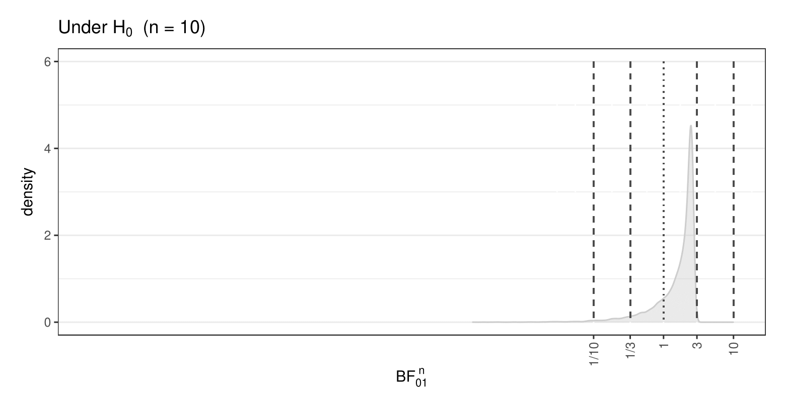
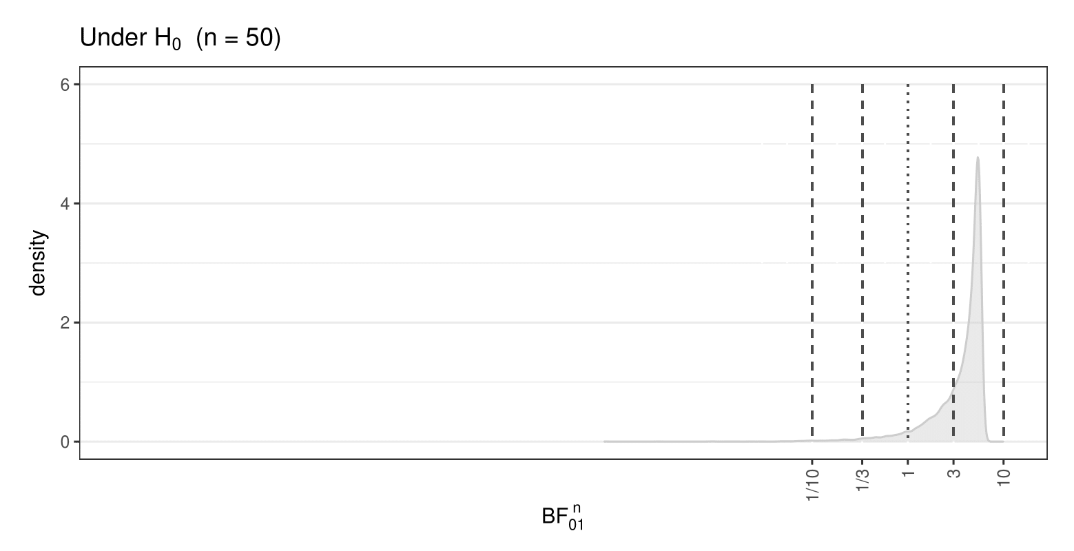
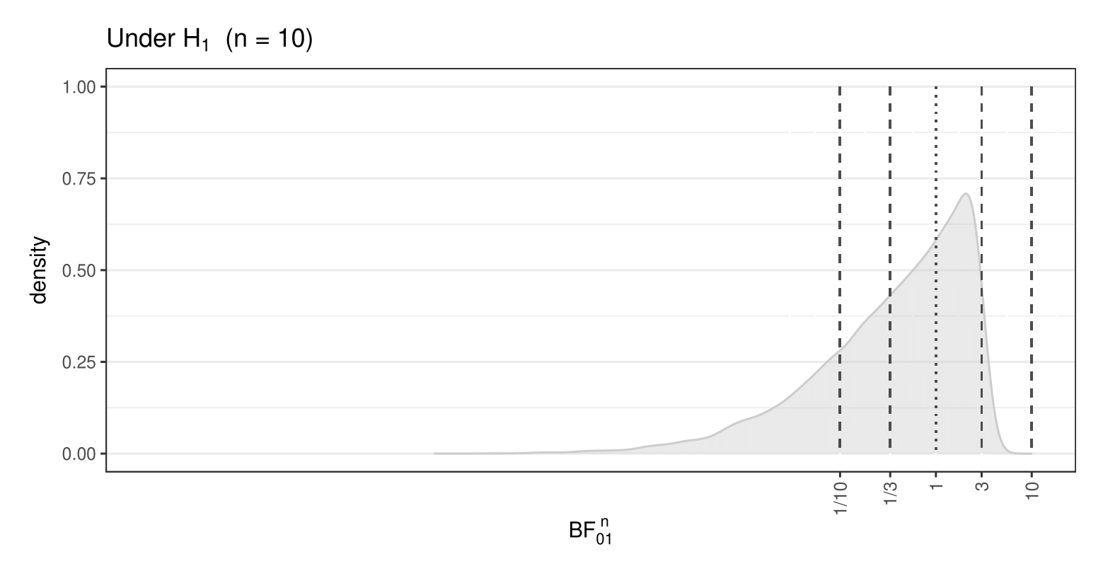
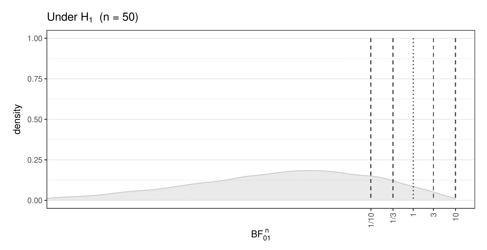
Figure 2: Two-node chain component: Predictive distribution of $\textnormal{log${}_{10}$ BF}_{01}^{n}$ under $H_{0}$ and $H_{1}$ for sample sizes $n=10$ and $n=50$. Vertical lines represent BF thresholds $1/10,1/3,1,3,10$.

Table 2: Two-node chain component. Predictive probabilities of $BF_{01}^{n}$ resulting in “moderate” or “strong-to-extreme” evidence in favor of the true hypothesis $H_{0}$ and $H_{1}$, for sample sizes $n\in\{10,50,100\}$.

True		$n$		Moderate	Strong-to-extreme
		$10$		0.00%	0.00%
$H_{0}$		$50$		73.64%	0.00%
		$100$		84.39%	2.10%
		$10$		18.5%	0.23%
$H_{1}$		$50$		7.70%	82.9%
		$100$		0.16%	96.2%

Consider now the probabilities of DCE as in Equations (30) and (31). We compute $p^{DC}_{0}(k_{0},n)$ and $p^{DC}_{1}(k_{1},n)$ for $k_{0}=k_{1}=k$ by varying $k\in\{3,6,10\}$, and for a grid of sample sizes $n\in\{1,2,\dots,1000\}$. The behavior of the two probabilities as a function of $n$ is summarized in the first two plots of Figure 3 where each curve refers to one value of $k$ (from dark to light grey for increasing levels of the threshold). Consider for instance $p^{DC}_{0}(k_{0},n)$: this probability exceeds 80% when $k=3$ for a sample size $n=100$, consistently with the results of Table 2. When instead $k=6$, the same sample size only guarantees that $p^{DC}_{0}(k_{0},n)$ is approximately equal to $65\%$; moreover, to reach a level of $80\%$ the sample size must increase to about $n=400$. Notice that $p^{DC}_{0}(k_{0}=10,n)$ is zero for $n$ up to 150; this explains the elbow in the bottom panel of Figure 3.

A similar behavior is observed for $p^{DC}_{1}(k_{1},n)$, where however the distance between the three curves is much smaller, especially for moderate-to-large values of $n$. This is coherent with the results in Figure 2 which suggest that the area to the left of 1/10 of the BF is already appreciable for small values of $n$ such as 10. In addition the area to the right of $k=3$ or $k=10$ are somewhat similar (and small) which explains the reason why the curves for the probabilities of DCE are close. Finally, the bottom panel of Figure 3 reports the overall probability of DCE in Equation (31), which averages $p^{DC}_{0}(k_{0},n)$ and $p^{DC}_{1}(k_{1},n)$ with $P(H_{0})=P(H_{1})=0.5$ following Equation (33).

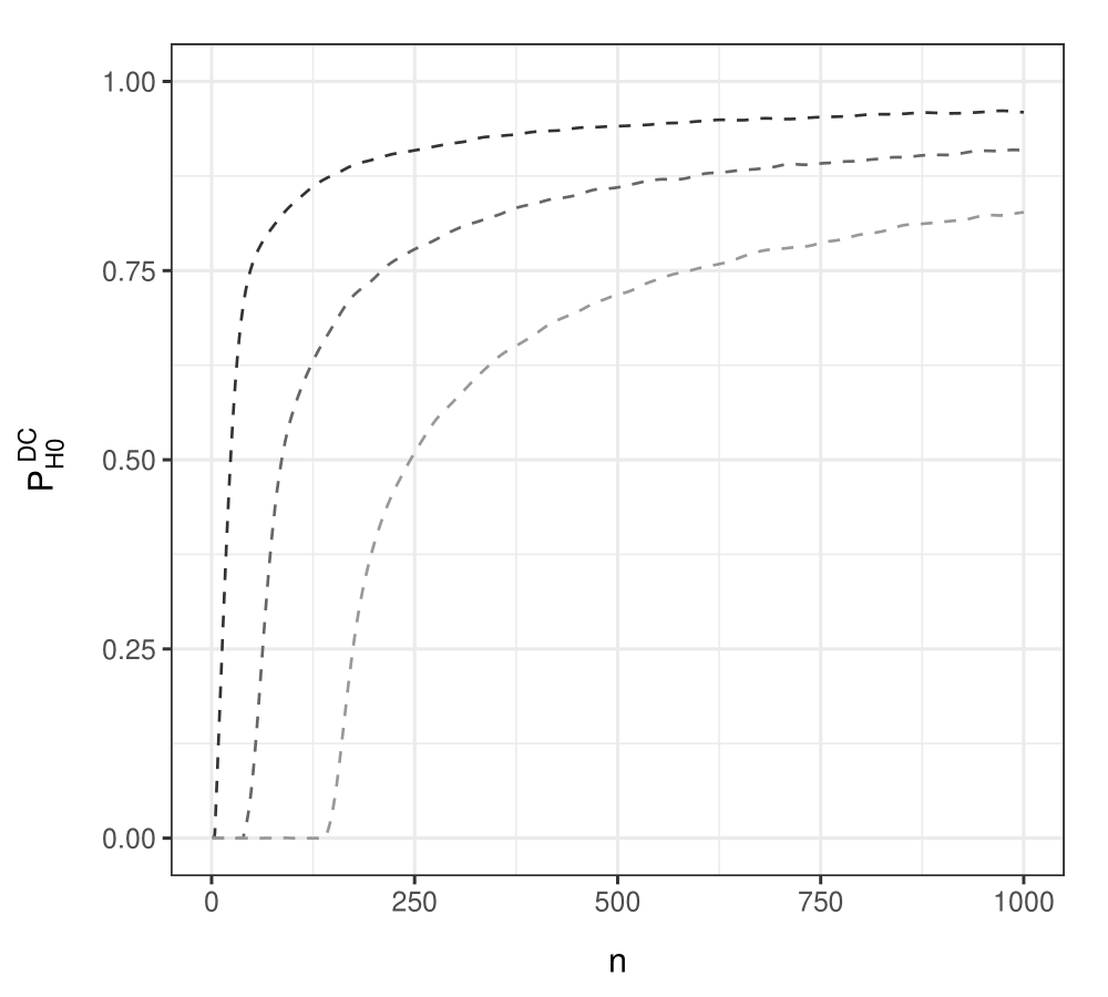
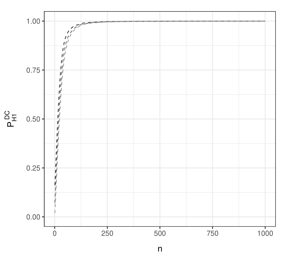
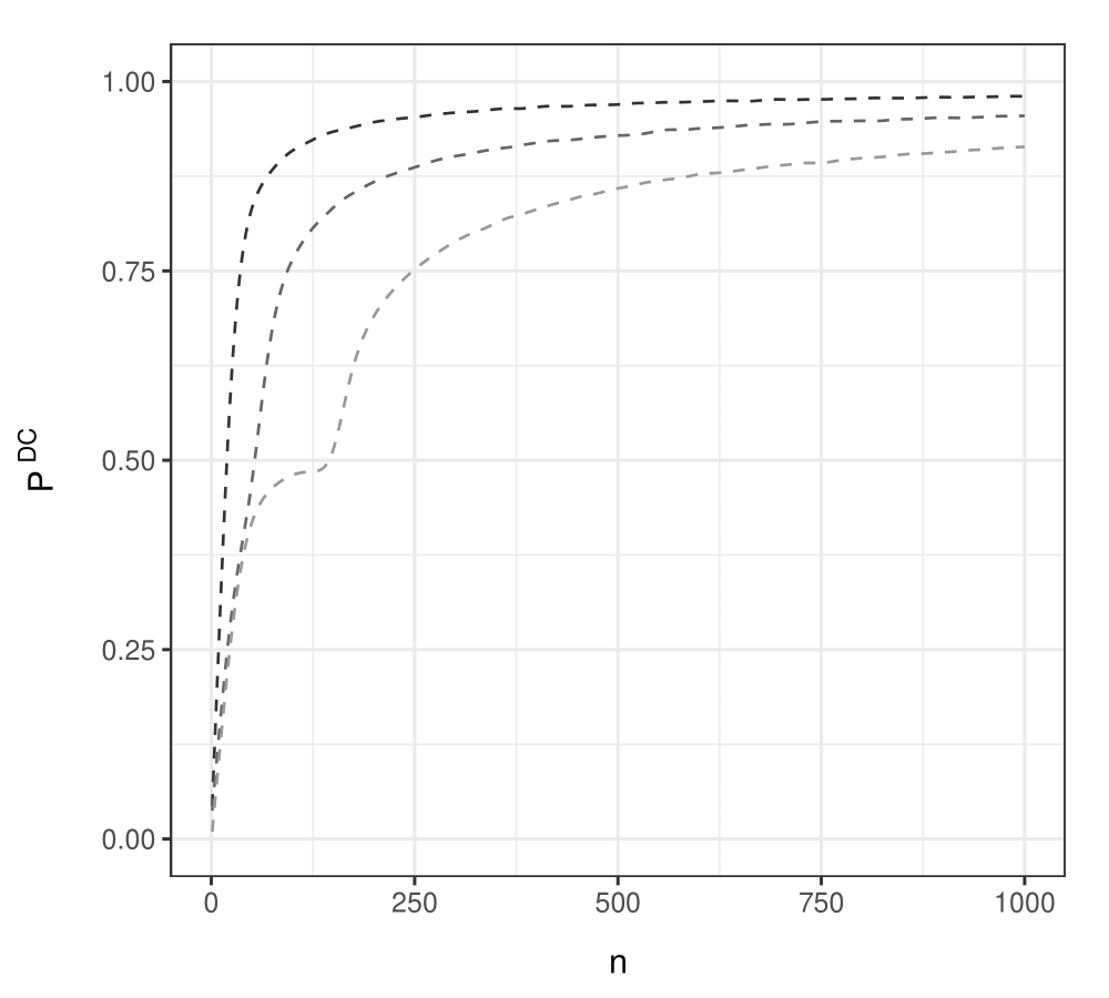
Figure 3: Two-node chain component: Probability of Decisive and Correct (DC) evidence in favour of $H_{0}$, $H_{1}$ and overall probability (from top to bottom plots) as a function of the sample size $n$, for different values of $k\in\{3,6,10\}$ (from dark to light grey) and $k_{0}=k_{1}=k$.

We now move to SSD and obtain the optimal sample size $n_{uv}^{*}$ for an intervention on $u$ based on (32). The latter quantity is computed for each value of the BF threshold $k\in\{3,6,10\}$ and for distinct thresholds for the probability of DCE $\zeta\in[0.5,\dots,0.95]$. Results are summarized in Figure 4 which reports the behavior of $n_{uv}^{*}$ as a function of $\zeta$ for the three increasing levels of $k$ (from dark to light gray). Clearly, the optimal sample size required for DCE increases with the threshold $\zeta$. The behavior of the three curves as $k$ varies is similar; however it becomes much steeper beyond $\zeta=0.85$ for $k=10$ (the cutoff which separates moderate from strong evidence). As an example, if we fix $\zeta=0.8$, we obtain an optimal sample size $n_{uv}^{*}\simeq 50$ for $k=3$, and this value triples when $k=6$ and reaches $n_{uv}^{*}\simeq 300$ for $k=10$. The latter sample size would instead guarantee a probability of DCE higher than $95\%$ when $k=3$.

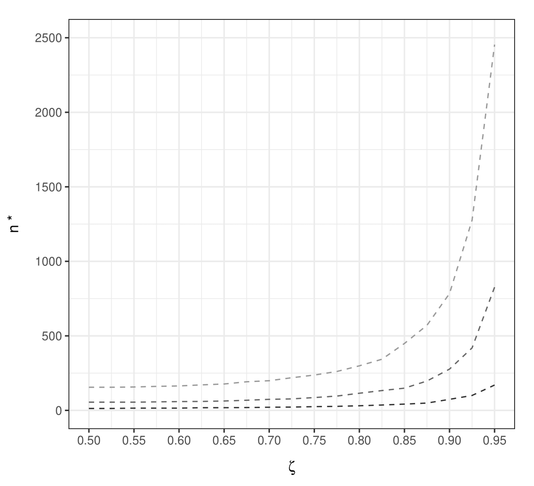
Figure 4: Two-node chain component: Optimal sample size $n_{uv}^{*}=n^{*}$ as a function of threshold $\zeta\in[0.50,0.95]$ for different values of $k\in\{3,6,10\}$ (from dark to light grey) and $k_{0}=k_{1}=k$.

4.2 Riboflavin data

In this section we apply our strategy for sample size determination to a data set about riboflavin (vitamin B2) production by Bacillus subtilis. The dataset is publicly available within the R package [53] hdi and includes $q=4089$ variables, namely the logarithm of the riboflavin production rate and the log-expression level of $4088$ genes that cover essentially the whole genome of Bacillus subtilis. The sample size is $N=71$. This observational dataset was analyzed by Maathuis et al. [40] to infer causal effects on the riboflavin production rate due to single gene manipulations. To this end the authors first estimate a CPDAG using the PC algorithm [64]. Then, using do-calculus theory, they provide an estimate of the causal effect on the riboflavin rate following an hypothetical intervention on each of the $4088$ nodes. Each causal effect is not unique in general because it depends on the specific set of parents of the node (also called adjustment set), and ultimately on the underlying DAG structure; see also Maathuis et al. [40, Algorithm 1]. Since typically many DAGs are compatible with the input CPDAG, a collection of possible causal effects (and eventually the corresponding average) is finally provided by their procedure.

We take a different course of action and apply our method to estimate the optimal sequence of manipulated variables and corresponding sample sizes as in Section 3. We start from an input CPDAG $\mathcal{E}$ estimated using the PC algorithm with the tuning parameter $\alpha$ set at level $0.01$. We then fix the threshold for the probability of DCE $\zeta=0.8$, while $k_{0}=k_{1}=6$. Recall now that our objective is SSD for an intervention needed to orient those edges which are undirected in the input CPDAG. Since undirected edges can only occur between (two ore more) nodes belonging to the same chain component, we focus on those chain components whose size is larger than one. Figure 5 summarizes the distribution of the size of chain components in the input CPDAG $\mathcal{E}$. Most of these (about $80\%$) have size equal to one, in which case there are no edges whose orientation needs to be determined. We then implement our method on each of the remaining chain components separately. As an example, Figure 6 reports two chain component sub-graphs $\mathcal{G}_{1},\mathcal{G}_{2}$. with the corresponding Best size Optimal Sequences of manipulated variables (BOS) represented as grey nodes. For $\mathcal{G}_{1}$ there are actually two optimal sequences according to Definition 3.1, namely $S_{1}=(2,3)$ and $S_{2}=(3,4)$, as we report in Table 3 with the corresponding optimal sample sizes computed as in (2). Clearly $S_{2}$ is the BOS because the total sample size under $S_{2}$ is smaller than under $S_{1}$. On the other hand, there is only one optimal sequence for $\mathcal{G}_{2}$, whose corresponding optimal sample size is $130$ (see again Table 3).

As an overall summary, we also report in Table 4, for each size of the chain components of $\mathcal{E}$ and size of the BOS, the corresponding average total sample size (Average $N^{*}$) and average sample size per intervention (Average $n^{*}$), with the average computed across sequences of manipulated variables. It appears that while in general the number of interventions needed for edge orientation (Size of sequence $S^{*}$) increases with the size of the chain component, the total sample size is not typically higher for larger (chain components and) sizes of $S^{*}$; compare for instance $s=4$ and $s=5$. In addition, the average sample size per intervention, for each given value of $s$ for which different sizes of $S^{*}$ are observed, is smaller for those sequences of manipulated variables having larger sizes. Accordingly, while more interventions are needed to orient edges in chain components of larger dimension, the (optimal) number of interventional data (sample size) required by each intervention is in general smaller. This suggests the existence of a trade-off between the number of manipulated variables and the optimal sample size per intervention.

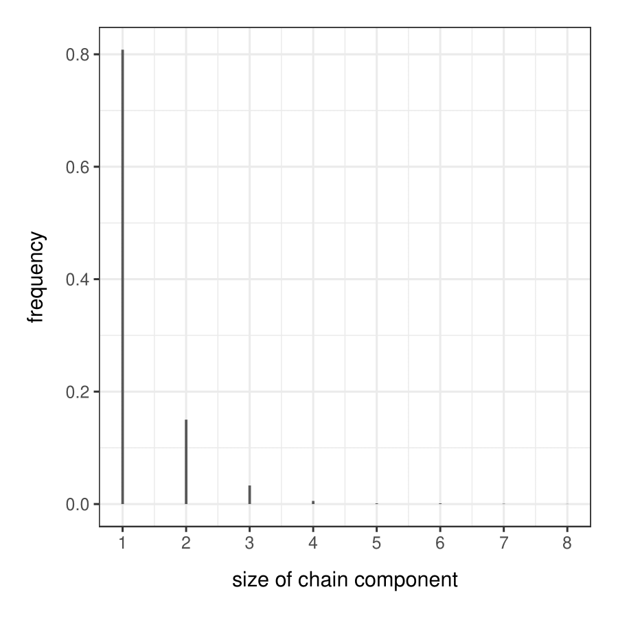
Figure 5: Riboflavin data: Distribution of the size of chain components in the estimated CPDAG.

$\mathcal{G}_{1}$			$\mathcal{G}_{2}$

Figure 6: Riboflavin data: Two chain-component sub-graphs, $\mathcal{G}_{1},\mathcal{G}_{2}$, with grey dots representing BOS manipulated variables.

Table 3: Riboflavin data: Optimal sequences of manipulated nodes and corresponding sample sizes for each of the two chain-component sub-graphs, $\mathcal{G}_{1},\mathcal{G}_{2}$ in Figure 6.

	Optimal sequence of nodes	Optimal sample size
$\mathcal{G}_{1}$	$S_{1}=(2,3)$	$\bm{n}^{*(1)}=(28,88)$
	$S_{2}=(3,4)$	$\bm{n}^{*(2)}=(4,86)$
$\mathcal{G}_{2}$	$S_{1}=2$	$\bm{n}^{*(1)}=130$

Table 4: Riboflavin data: average total sample size (Average $N^{*}$) and average sample size per manipulated variable (Average $n^{*}$) cross-classified by size of chain component of the input CPDAG and size of the sequence of manipulated variables $S^{*}$.

Size of chain component		$s=2$		$s=3$			$s=4$			$s=5$
Size of sequence $S^{*}$		1		1	2		1	2		2
Average $N^{*}$		48.3		131.4	100.0		241.3	248.4		81.0
Average $n^{*}$		48.3		131.4	50.0		241.3	124.2		40.5

$s=6$			$s=7$		$s=8$
2	3		3		4
67.0	37.0		65.5		117.0
33.5	12.3		21.8		29.3

5 Discussion

Observational data cannot distinguish in general among different DAG-models representing the same conditional independence assertions. This is a serious drawback for causal inference which is predicated on a given DAG representing the data generating process, as required by do-calculus theory. Intervention experiments, leading to the collection of interventional data, can greatly improve the structure learning process. So far most works in active learning have concentrated on efficient algorithms to select target variables to intervene upon in order to guarantee identification of the underlying causal DAG, starting from a Markov equivalence class of DAGs. Interventions on variables help decide how to orient undirected edges which are present in the CPDAG representative of the equivalence class. However the actual decision is based on sampling data, as in the independence test between a target variable and one of its neighbors. Active learning involves therefore two aspects, one is algorithmic and uses graph-based notions for the selection of the target variables, and the other one is statistical and uses samples of interventional data, possibly coupled with external information, which may include previously collected observational data or substantive domain knowledge. In this context, a question which has so far been neglected is the determination of the sample size of the interventional data required to achieve desirable inferential properties. This paper addresses this issue with regard to the problem of edge orientation, which is framed as a test of hypothesis between two competing DAG structures. Specifically, we use the Bayes factor as a measure of evidence, and for a given sequence of optimally specified intervention variables, we determine the corresponding collection of sample sizes which will produce decisive and correct evidence in favor of the true causal-model hypothesis at each intervention.

Our method takes as input an equivalence class of DAGs, equivalently its representative CPDAG, which typically has been estimated from an observational dataset. It does not accommodate for estimation uncertainty, as most active learning methods do. In principle the posterior distribution over the space of Markov equivalence classes, see e.g. Castelletti et al. [6], could be of some help to evaluate the strength of the evidence in favor of the chosen CPDAG, possibly the highest posterior probability model. Operationally, however, one would still need a single sequence of variables to manipulate in order to perform sample size determination (SSD), and it is far from clear how standard Bayesian Model Averaging techniques could be used in a fruitful way.

Our method for SSD is based on a sequence of manipulated variables arising from a batch intervention experiment. A sequential approach would instead proceed by choosing the intervention nodes one at a time and collecting new data after each intervention [66, 28]. In this way, the optimal sample size associated with a target node could be computed, at each stage, using all the samples collected up to that step, thus increasing the amount of information used for prediction at the design level. Another advantage of the sequential method is to alleviate the danger inherent in the choice of the starting Markov equivalence class, namely that the true DAG could be outside the class. Hauser & Bühlmann [26] investigate this aspect and illustrate by simulation that methods that do take into account observational as well as interventional data show a better performance in recovering the true data-generating DAG. We observe that our method could be tailored to a sequential setup by incorporating in the predictive distribution of the BF not only the initial observational data but also the newly interventional observations collected at each step.

In our procedure experimental data are generated under hard interventions and in the absence of latent variables. Under hard (or perfect) interventions, dependencies between targeted variables and their direct causes are removed. This assumption may not hold in some settings where dependencies can only be altered without being fully deleted. An instance is genomic medicine, where gene manipulation through repression or activation of selected genes is performed to better understand the complex functioning of the pathway. Intervention experiments for gene regulation are meant to be perfect but in practice may not be uniformly successful across a cell population, in which case the dependence between manipulated genes and their direct causes in the network is only weakened but maintained. Identifiabilty of causal DAGs from soft interventions is investigated from a theoretical perspective by Yang et al. [71] who propose a consistent algorithm for DAG structure learning.

Finally, our theoretical framework is that of a causally sufficient system with no latent confounders, selection bias, or feedback. Some works on structural learning try to alleviate these limitations; see for instance Frot et al. [22] and Squires et al. [65].

Appendix A Priors for DAG model comparison and Bayes Factor computation

Our elicitation scheme for parameter priors under a general Gaussian DAG model is based on the procedure introduced by Geiger & Heckerman [23] (G&H). This is used both to construct the analysis prior and the design prior. The former is needed to obtain the Bayes factor, whose predictive distribution is generated under the latter.

A.1 General assumptions

The method of G&H is based on a set of assumptions which drastically simplifies the elicitation of priors; additionally it ensures compatibility of priors across DAG models, so that DAGs belonging to the same equivalence class score the same marginal likelihood. This feature is important when DAG model comparison is based on observational data, because the latter cannot distinguish in general among Markov equivalent DAGs. This however is no longer the case when interventional data are also employed, as we do in Section 2.2.

The method assumes some regularity conditions on the likelihood, namely complete model equivalence, regularity and likelihood modularity which are satisfied by any Gaussian model. In addition, two assumptions on the prior distributions are introduced. The first assumption (prior modularity) states that, for any two distinct DAG models with the same set of parents for vertex $j$, the prior for the node-parameter $\bm{\theta}_{j}$ must be the same under both models. Moreover, the second assumption (global parameter independence) states that for every DAG model $\mathcal{D}$, the parameters $\{\bm{\theta}_{j};\,j=1,\ldots,q\}$ should be a priori independent, that is

$$p(\bm{\theta}\,|\,\mathcal{D})=\prod_{j=1}^{q}p(\bm{\theta}_{j}\,|\,\mathcal{D}).$$

Based on these assumptions, Theorem 1 of Geiger & Heckerman [23] shows that the parameter priors of all DAG models are completely determined by a unique prior on the parameter of any of the (equivalent) complete DAGs.

Specifically, in the zero-mean Gaussian framework, all priors across DAG models can be shown to be driven by a single Wishart distribution on an unconstrained precision matrix. Most importantly, a direct consequence of the method is that each marginal data distribution in Equation (22) corresponds to the marginal data distribution computed under any complete DAG model; see next section for more details.

A.2 Marginal data distributions and Bayes Factor

Consider a multivariate Gaussian model of the form

$$\begin{aligned} \bm{x}_{1},\dots,\bm{x}_{n}\,|\,\bm{\Omega}&\overset{\textnormal{iid}}{\sim}\mathcal{N}_{T}\left(\bm{0},\bm{\Omega}^{-1}\right)\\ \bm{\Omega}&\sim\mathcal{W}_{T}(a,\bm{U}),\end{aligned}$$ (34)

where $\mathcal{W}_{T}(a,\bm{U})$ denotes a Wishart distribution having expectation $a\bm{U}^{-1}$ and $a>T-1$. Let also $\bm{S}=\sum_{h=1}^{n}\bm{x}_{h}\bm{x}_{h}^{\top}$. The marginal data distribution restricted to variables in $A\subseteq\{1,\dots,T\}$ is given by

$$m(\bm{X}_{A})=\frac{\prod_{j=1}^{|A|}\Gamma\left(\frac{a-|\bar{A}|+n+1-j}{2}\right)}{\prod_{j=1}^{|A|}\Gamma\left(\frac{a-|\bar{A}|+1-j}{2}\right)}\frac{\left|\bm{U}_{A,A}\right|^{\frac{a-|\bar{A}|}{2}}}{\left|\bm{U}_{A,A}+\bm{S}_{A,A}\right|^{\frac{a-|\bar{A}|+n}{2}}},$$

where $\bm{U}_{A,A}$ denotes the sub-matrix of $\bm{U}$ with rows and columns indexed by $A$ and $\bar{A}=\{1,\dots,T\}\setminus A$; see for instance Consonni & La Rocca [10, Equation 12]. Moreover for simplicity in this section we omit superscript $n$ from data matrices. Under the Gaussian setting of Section 2.3, the BF in Equation (22) can be evaluated using the marginal likelihood (A.2) for $A=u$, $A=v$ and $A=\{u,v\}$. We thus obtain

$$m(\bm{X}_{u})=\frac{\Gamma\left(\frac{a-(T-1)+n}{2}\right)}{\Gamma\left(\frac{a-(T-1)}{2}\right)}\frac{\left|\bm{U}_{u,u}\right|^{\frac{a-(T-1)}{2}}}{\left|\bm{U}_{u,u}+\bm{S}_{u,u}\right|^{\frac{a-(T-1)+n}{2}}}$$

and similarly for $A=v$, while for $A=\{u,v\}$,

$$m(\bm{X}_{u,v}) = \frac{\Gamma\left(\frac{a-(T-2)+n}{2}\right)}{\Gamma\left(\frac{a-(T-2)}{2}\right)}\frac{\Gamma\left(\frac{a-(T-2)+n-1}{2}\right)}{\Gamma\left(\frac{a-(T-2)-1}{2}\right)}$$ (37)

$$\cdot \frac{\left|\bm{U}_{\{u,v\},\{u,v\}}\right|^{\frac{a-(T-1)}{2}}}{\left|\bm{U}_{\{u,v\},\{u,v\}}+\bm{S}_{\{u,v\},\{u,v\}}\right|^{\frac{a-(T-1)+n}{2}}}.$$

Therefore, the BF in (22) reduces to

$$\textnormal{BF}_{01}^{n} = \frac{\Gamma\left(\frac{a-(T-1)+n}{2}\right)}{\Gamma\left(\frac{a-(T-1)}{2}\right)}\cdot\frac{\Gamma\left(\frac{a-(T-2)}{2}\right)}{\Gamma\left(\frac{a-(T-2)+n}{2}\right)}$$ (38)

$$\cdot \frac{\left[\bm{U}_{u,u}\bm{U}_{v,v}\right]^{\frac{a-(T-1)}{2}}}{\left|\bm{U}_{\{u,v\},\{u,v\}}\right|^{\frac{a-(T-2)}{2}}}\cdot\frac{\left|\bm{U}_{\{u,v\},\{u,v\}}+\bm{S}_{\{u,v\},\{u,v\}}\right|^{\frac{a-(T-2)+n}{2}}}{\left[(\bm{U}_{u,u}+\bm{S}_{u,u})(\bm{U}_{v,v}+\bm{S}_{v,v})\right]^{\frac{a-(T-1)+n}{2}}}.$$

So far results were obtained under a subjective prior on $\bm{\Omega}$. We now consider an objective framework based on the notion of Fractional Bayes Factor (FBF) [45]. Specifically, we start from the default objective prior

$$p^{D}(\bm{\Omega})\propto|\bm{\Omega}|^{\frac{a_{\Omega}-T-1}{2}}.$$ (39)

Let now $\bar{\bm{S}}=\frac{1}{n}\bm{S}$. The (data dependent) fractional prior on $\bm{\Omega}$ is defined as

$$p^{F}(\bm{\Omega})\propto\left\{p(\bm{X}\,|\,\bm{\Omega})\right\}^{b}p^{D}(\bm{\Omega}),$$

where $b\in(0,1)$ is typically chosen as the smallest value s.t. the fractional prior is proper. After some calculations we obtain

$$\bm{\Omega}\sim\mathcal{W}_{T}(a_{\Omega}+n_{0},n_{0}\bar{\bm{S}}),$$

where $n_{0}=bn$, which is proper provided $a_{\Omega}+n_{0}>T-1$; see Consonni & La Rocca [10] for full details. Also, the posterior distribution of $\bm{\Omega}$ is

$$p(\bm{\Omega}\,|\,\bm{X}) \propto \left\{p(\bm{X}\,|\,\bm{\Omega})\right\}^{1-b}p^{F}(\bm{\Omega})$$

$$= \left\{p(\bm{X}\,|\,\bm{\Omega})\right\}p^{D}(\bm{\Omega}).$$

The FBF is obtained by specializing (38) with

$$a\mapsto a_{\Omega}+n_{0},\quad n\mapsto n-n_{0},$$

$$\bm{U}\mapsto\frac{n_{0}}{n}\bm{S},\quad\bm{S}\mapsto\frac{n-n_{0}}{n}\bm{S},$$

which after some calculations leads to

$$\textnormal{BF}_{01}^{n} = \frac{\Gamma\left(\frac{a_{\Omega}-(T-1)+n}{2}\right)}{\Gamma\left(\frac{a_{\Omega}+n_{0}-(T-1)}{2}\right)}\cdot\frac{\Gamma\left(\frac{a_{\Omega}+n_{0}-(T-2)}{2}\right)}{\Gamma\left(\frac{a_{\Omega}-(T-2)+n}{2}\right)}\cdot\left(\frac{n_{0}}{n}\right)^{-1}\left[\frac{\left|\bm{S}_{\{u,v\},\{u,v\}}\right|}{\bm{S}_{u,u}\bm{S}_{v,v}}\right]^{\frac{n-n_{0}}{2}}.$$

Now notice that

$$\left|\bm{S}_{\{u,v\},\{u,v\}}\right|=\sum_{h=1}^{n}x_{h,u}^{2}\sum_{h=1}^{n}x_{h,v}^{2}-\left(\sum_{h=1}^{n}x_{h,u}x_{h,v}\right)^{2}$$

and

$$\bm{S}_{u,u}=\sum_{h=1}^{n}x_{h,u}^{2},\quad\bm{S}_{v,v}=\sum_{h=1}^{n}x_{h,v}^{2}.$$

Therefore, we can write

$$\begin{aligned} \frac{\left|\bm{S}_{\{u,v\},\{u,v\}}\right|}{\bm{S}_{u,u}\bm{S}_{v,v}}&=1-\frac{\left(\sum_{h=1}^{n}x_{h,u}x_{h,v}\right)^{2}}{\sum_{h=1}^{n}x_{h,u}^{2}\sum_{h=1}^{n}x_{h,v}^{2}}\\ &=1-\left(r_{u,v}^{n}\right)^{2}\end{aligned}$$ (40)

where $r_{u,v}^{n}$ denotes the sample correlation coefficient between $X_{u}$ and $X_{v}$. In the sequel we choose $a_{\Omega}=T-1$ so that the prior is proper even with a training sample size $n_{0}$ equal to one, and we obtain

$$\begin{aligned} \textnormal{BF}_{01}^{n}&=\frac{1}{\sqrt{\pi}}\frac{\Gamma\left(\frac{n}{2}\right)}{\Gamma\left(\frac{n+1}{2}\right)}n\left[1-(r_{uv}^{n})^{2}\right]^{\frac{n-1}{2}}.\end{aligned}$$ (41)

A.3 Posterior distribution of DAG model parameters

The design prior for $(\bm{L}_{u,v},\bm{D}_{v,v})$ that we adopt in Section 2.3.2 corresponds to the posterior $p(\bm{L}_{u,v},\bm{D}_{v,v}\,|\,\bm{Z},\mathcal{D}_{1})$. The latter can be recovered from the posterior on $\bm{\Omega}=\bm{\Sigma}^{-1}$, the (unconstrained) precision matrix of a complete DAG, following the procedure of G&H, which we detail below.

Let $\mathcal{D}$ be an arbitrary DAG and let $\prec j\succ\,=\mathrm{pa}(j)$, and $\prec j\,]=\mathrm{pa}(j)\times j$. Consider the (Cholesky) re-parameterization $\bm{\Omega}\mapsto(\bm{L},\bm{D})$ where, for $j\in\{1,\dots,q\}$,

$$\bm{D}_{jj}=\bm{\Sigma}_{jj\,|\,\mathrm{pa}_{\mathcal{D}}(j)},\quad\bm{L}_{\prec j\,]}=-\bm{\Sigma}^{-1}_{\prec j\,\succ}\bm{\Sigma}_{\prec j\,]}$$

For each node $j\in\{1,\dots,q\}$, let $\big{\{}\bm{D}_{jj},\bm{L}_{\prec j\,]}\big{\}}$ be the parameters associated to node $j$, and identify a complete DAG $\mathcal{D}^{C(j)}$ such that $\mathrm{pa}_{\mathcal{D}^{C(j)}}(j)=\mathrm{pa}_{\mathcal{D}}(j)$. Let $\big{\{}\bm{D}_{jj}^{C(j)},\bm{L}_{\prec j\,]}^{C(j)}\big{\}}$ be the parameters of node $j$ under the complete DAG $\mathcal{D}^{C(j)}$. We then assign to $\left\{\bm{D}_{jj},\bm{L}_{\prec j\,]}\right\}$ the same prior of $\big{\{}\bm{D}_{jj}^{C(j)},\bm{L}_{\prec j\,]}^{C(j)}\big{\}}$. However, because our interest is in obtaining the posterior of DAG parameters $(\bm{D},\bm{L})$, we can compute first the posterior on the unconstrained $\bm{\Omega}$, which by conjugacy is still Wishart, and then recover the posterior on $(\bm{D},\bm{L})$.

Consider a random sample of size $N$, $\bm{z}_{1},\dots,\bm{z}_{N}$, with $\bm{z}_{i}=(x_{i,1},\dots,x_{i,q})^{\top}$ and $\bm{z}_{i}\,|\,\bm{\Omega}\overset{\textnormal{iid}}{\sim}\mathcal{N}_{q}(\bm{0},\bm{\Omega}^{-1})$, $i=1,\dots,N$, where $\bm{\Omega}$ is unconstrained. Let also $\bm{Z}$ be the $(N,q)$ data matrix, obtained by row-binding the individual $\bm{z}_{i}^{\top}$’s. The posterior distribution of $\bm{\Omega}$ computed under the default prior (39) is given by

$$\bm{\Omega}\,|\,\bm{Z}\sim\mathcal{W}_{T}(a_{\Omega}+n,\bm{Z}^{\top}\bm{Z}).$$

To obtain draws from the posterior of $(\bm{L}_{u,v},\bm{D}_{v,v})$, set $\left(\bm{\Sigma}_{\{u,v\},\{u,v\}}\right)^{-1}:=\bm{Q}_{u,v}$, and using properties of the Wishart distribution deduce

$$\quad\quad\bm{Q}_{\{u,v\}}\sim\mathcal{W}_{2}\left(a_{\Omega}+N-(T-2),\bm{S}_{\{u,v\},\{u,v\}}\right);$$ (42)

see Press [52, Thm 5.1.4] and Consonni & La Rocca [10, Section 2.1]. Consider now a draw from (42) and compute $\bm{\Sigma}_{\{u,v\},\{u,v\}}$. Finally recover

$$\bm{L}_{u,v}=-\left(\bm{\Sigma}_{\{u,v\},\{u,v\}}\right)^{-1}\bm{\Sigma}_{u,v},\quad\bm{D}_{v,v}=\bm{\Sigma}_{v\,|\,u},$$

where $\bm{\Sigma}_{v\,|\,u}=\bm{\Sigma}_{v,v}-(\bm{\Sigma}_{v,u})^{2}\bm{\Sigma}_{u,u}^{-1}$.

References

- Adcock [1997] Adcock, C. J. (1997). Sample size determination: A review. J. R. Stat. Soc. D. Stat. 46 261–283.
- Andersson et al. [1997] Andersson, S. A., Madigan, D. & Perlman, M. D. (1997). A characterization of Markov equivalence classes for acyclic digraphs. Ann. Statist. 25 505–541.
- Andersson et al. [2001] Andersson, S. A., Madigan, D. & Perlman, M. D. (2001). Alternative Markov properties for chain graphs. Scand. J. Stat. 28 33–85.
- Castelletti & Consonni [2020] Castelletti, F. & Consonni, G. (2020). Discovering causal structures in bayesian gaussian directed acyclic graph models. J. R. Stat. Soc. Ser. A. Stat. Soc. 183 1727–1745.
- Castelletti & Consonni [2021] Castelletti, F. & Consonni, G. (2021). Bayesian inference of causal effects from observational data in Gaussian graphical models. Biometrics 77 136–149.
- Castelletti et al. [2018] Castelletti, F., Consonni, G., Della Vedova, M. & Peluso, S. (2018). Learning Markov equivalence classes of directed acyclic graphs: An objective Bayes approach. Bayesian Anal. 13 1235–1260.
- Castelo & Perlman [2004] Castelo, R. & Perlman, M. D. (2004). Learning essential graph Markov models from data. In Advances in Bayesian networks, vol. 146 of Stud. Fuzziness Soft Comput. Springer, Berlin, 255–269.
- Chaloner & Verdinelli [1995] Chaloner, K. & Verdinelli, I. (1995). Bayesian experimental design: A review. Statist. Sci. 10 273–304.
- Chickering [2002] Chickering, D. M. (2002). Learning equivalence classes of Bayesian-network structures. J. Mach. Learn. Res. 2 445–498.
- Consonni & La Rocca [2012] Consonni, G. & La Rocca, L. (2012). Objective Bayes factors for Gaussian directed acyclic graphical models. Scand. J. Stat. 39 743–756.
- Consonni & Veronese [2008] Consonni, G. & Veronese, P. (2008). Compatibility of prior specifications across linear models. Statist. Sci. 23 332–353.
- Cowell et al. [1999] Cowell, R. G., Dawid, P. A., Lauritzen, S. L. & Spiegelhalter, D. J. (1999). Probabilistic Networks and Expert Systems. New York: Springer.
- DasGupta [1996] DasGupta, A. (1996). 29 review of optimal bayes designs. In Design and Analysis of Experiments, vol. 13 of Handbook of Statistics. Elsevier, 1099–1147.
- Dawid [2011] Dawid, A. P. (2011). Posterior model probabilities. In P. S. Bandyopadhyay & M. Forster, eds., Philosophy of Statistics. Elsevier, Amsterdam, 607–630.
- Dawid & Lauritzen [1993] Dawid, A. P. & Lauritzen, S. L. (1993). Hyper Markov laws in the statistical analysis of decomposable graphical models. Ann. Statist. 21 1272–1317.
- Dawid & Lauritzen [2001] Dawid, A. P. & Lauritzen, S. L. (2001). Compatible prior distributions. In E. George, ed., Bayesian methods with applications to science, policy and official statistics: Selected Papers from ISBA 2000, the Sixth World Meeting of the International Society for Bayesian Analysis. 109–118.
- De Santis [2004] De Santis, F. (2004). Statistical evidence and sample size determination for bayesian hypothesis testing. J. Statist. Plann. Inference 124 121–144.
- Drton & Eichler [2006] Drton, M. & Eichler, M. (2006). Maximum likelihood estimation in Gaussian chain graph models under the alternative Markov property. Scand. J. Stat. 33 247–257.
- Eberhardt [2008] Eberhardt, F. (2008). Almost optimal intervention sets for causal discovery. In Proceedings of the Twenty-Fourth Conference on Uncertainty in Artificial Intelligence, UAI ’08. Arlington, Virginia, USA: AUAI Press, 161–168.
- Etzioni & Kadane [1993] Etzioni, R. & Kadane, J. B. (1993). Optimal experimental design for another’s analysis. J. Amer. Statist. Assoc. 88 1404–1411.
- Friedman [2004] Friedman, N. (2004). Inferring cellular networks using probabilistic graphical models. Science 303 799–805.
- Frot et al. [2019] Frot, B., Nandy, P. & Maathuis, M. H. (2019). Robust causal structure learning with some hidden variables. J. R. Stat. Soc. Ser. B. Stat. Methodol. 81 459–487.
- Geiger & Heckerman [2002] Geiger, D. & Heckerman, D. (2002). Parameter priors for directed acyclic graphical models and the characterization of several probability distributions. Ann. Statist. 30 1412–1440.
- Gelfand & Wang [2002] Gelfand, A. E. & Wang, F. (2002). A simulation-based approach to Bayesian sample size determination for performance under a given model and for separating models. Statist. Sci. 17 193–208.
- Hauser & Bühlmann [2012] Hauser, A. & Bühlmann, P. (2012). Characterization and greedy learning of interventional Markov equivalence classes of directed acyclic graphs. J. Mach. Learn. Res. 13 2409–2464.
- Hauser & Bühlmann [2014] Hauser, A. & Bühlmann, P. (2014). Two optimal strategies for active learning of causal models from interventional data. Int. J. Approx. Reason. 55 926–939.
- Hauser & Bühlmann [2015] Hauser, A. & Bühlmann, P. (2015). Jointly interventional and observational data: estimation of interventional Markov equivalence classes of directed acyclic graphs. J. R. Stat. Soc. Ser. B. Stat. Methodol. 77 291–318.
- He & Geng [2008] He, Y. & Geng, Z. (2008). Active learning of causal networks with intervention experiments and optimal designs. J. Mach. Learn. Res. 9 2523–2547.
- He et al. [2013] He, Y., Jia, J. & Yu, B. (2013). Reversible MCMC on Markov equivalence classes of sparse directed acyclic graphs. Ann. Statist. 41 1742–1779.
- Hyttinen et al. [2013] Hyttinen, A., Eberhardt, F. & Hoyer, P. O. (2013). Experiment selection for causal discovery. J. Mach. Learn. Res. 14 3041–3071.
- Imbens [2020] Imbens, G. W. (2020). Potential outcome and directed acyclic graph approaches to causality: relevance for empirical practice in economics. J. Econ. Lit. 58 1129–1179.
- Jeffreys [1961] Jeffreys, H. (1961). Theory of Probability (3rd Edition). Oxford, University Press.
- Johnson & Rossell [2010] Johnson, V. E. & Rossell, D. (2010). On the use of non-local prior densities in Bayesian hypothesis tests. J. R. Stat. Soc. Ser. B. Stat. Methodol. 72 143–170.
- Kalisch & Bühlmann [2007] Kalisch, M. & Bühlmann, P. (2007). Estimating high-dimensional directed acyclic graphs with the pc-algorithm. J. Mach. Learn. Res. 8 613–636.
- Kass & Raftery [1995] Kass, R. E. & Raftery, A. E. (1995). Bayes factors. J. Amer. Statist. Assoc. 90 773–795.
- Koller & Friedman [2009] Koller, D. & Friedman, N. (2009). Probabilistic Graphical Models: Principles and Techniques. Adaptive computation and machine learning. MIT Press.
- Lauritzen [1996] Lauritzen, S. L. (1996). Graphical Models. Oxford University Press.
- Lindley [1972] Lindley, D. V. (1972). 1. Bayesian Statistics, a Review. 1–74.
- Lindley [1997] Lindley, D. V. (1997). The choice of sample size. J. R. Stat. Soc. D. Stat. 46 129–138.
- Maathuis et al. [2009] Maathuis, M. H., Kalisch, M. & Bühlmann, P. (2009). Estimating high-dimensional intervention effects from observational data. Ann. Statist. 37 3133–3164.
- Madigan et al. [1996] Madigan, D., Andersson, S. A., Perlman, M. D. & Volinsky, C. T. (1996). Bayesian model averaging and model selection for Markov equivalence classes of acyclic digraphs. Commun. Stat. - Theor. M. 25 2493–2519.
- Meganck et al. [2006] Meganck, S., Leray, P. & Manderick, B. (2006). Learning causal bayesian networks from observations and experiments: A decision theoretic approach. In V. Torra, Y. Narukawa, A. Valls & J. Domingo-Ferrer, eds., Modeling Decisions for Artificial Intelligence. Berlin, Heidelberg: Springer Berlin Heidelberg, 58–69.
- Muirhead [1982] Muirhead, R. (1982). Aspects of Multivariate Statistical Theory. John Wiley & Sons, Ltd.
- Nagarajan et al. [2013] Nagarajan, R., Scutari, M. & Lèbre, S. (2013). Bayesian Networks in R: With Applications in Systems Biology. Springer Publishing Company, Incorporated.
- O’Hagan [1995] O’Hagan, A. (1995). Fractional Bayes factors for model comparison. J. R. Stat. Soc. Ser. B. Stat. Methodol. 57 99–138.
- O’Hagan & Stevens [2001] O’Hagan, A. & Stevens, J. (2001). Bayesian assessment of sample size for clinical trials of cost-effectiveness. Med. Decis. Making 21 219–30.
- Pan & Banerjee [2021] Pan, J. & Banerjee, S. (2021). A unifying bayesian approach for sample size determination using design and analysis priors. arXiv preprint arXiv:2112.03509 .
- Pearl [2000] Pearl, J. (2000). Causality: Models, Reasoning, and Inference. Cambridge University Press, Cambridge.
- Pearl [2003] Pearl, J. (2003). Statistics and causal inference: A review. Test 281–345.
- Peng et al. [2020] Peng, S., Shen, X. & Pan, W. (2020). Reconstruction of a directed acyclic graph with intervention. Electron. J. Stat. 14 4133–4164.
- Peters & Bühlmann [2013] Peters, J. & Bühlmann, P. (2013). Identifiability of Gaussian structural equation models with equal error variances. Biometrika 101 219–228.
- Press [1982] Press, S. J. (1982). Applied multivariate analysis: using Bayesian and frequentist methods of inference. Krieger Publishing Company, Malabar, FL.
- R Core Team [2021] R Core Team (2021). R: A Language and Environment for Statistical Computing. R Foundation for Statistical Computing, Vienna, Austria.
- Raiffa & Schlaifer [1961] Raiffa, H. & Schlaifer, R. (1961). Applied Statistical Decision Theory. Harvard Business School Publications. Division of Research, Graduate School of Business Adminitration, Harvard University.
- Royall [1997] Royall, R. (1997). Statistical Evidence: A likelihood paradigm (1st ed.). Routledge.
- Royall [2000] Royall, R. (2000). On the probability of observing misleading statistical evidence. J. Amer. Statist. Assoc. 95 760–768.
- Sachs et al. [2005] Sachs, K., Perez, O., Pe’er, D., Lauffenburger, D. & Nolan, G. (2005). Causal protein-signaling networks derived from multiparameter single-cell data. Science 308 523–529.
- Sadeghi [2017] Sadeghi, K. (2017). Faithfulness of probability distributions and graphs. J. Mach. Learn. Res. 18 1–29.