Nest Your Adaptive Algorithm for Parameter-Agnostic
Nonconvex Minimax Optimization

Abstract

Adaptive algorithms like AdaGrad and AMSGrad are successful in nonconvex optimization owing to their parameter-agnostic ability – requiring no a priori knowledge about problem-specific parameters nor tuning of learning rates. However, when it comes to nonconvex minimax optimization, direct extensions of such adaptive optimizers without proper time-scale separation may fail to work in practice. We provide such an example proving that the simple combination of Gradient Descent Ascent (GDA) with adaptive stepsizes can diverge if the primal-dual stepsize ratio is not carefully chosen; hence, a fortiori, such adaptive extensions are not parameter-agnostic. To address the issue, we formally introduce a Nested Adaptive framework, NeAda for short, that carries an inner loop for adaptively maximizing the dual variable with controllable stopping criteria and an outer loop for adaptively minimizing the primal variable. Such mechanism can be equipped with off-the-shelf adaptive optimizers and automatically balance the progress in the primal and dual variables. Theoretically, for nonconvex-strongly-concave minimax problems, we show that NeAda with AdaGrad stepsizes can achieve the near-optimal $\widetilde{O}(\epsilon^{-2})$ and $\widetilde{O}(\epsilon^{-4})$ gradient complexities respectively in the deterministic and stochastic settings, without prior information on the problem’s smoothness and strong concavity parameters. To the best of our knowledge, this is the first algorithm that simultaneously achieves near-optimal convergence rates and parameter-agnostic adaptation in the nonconvex minimax setting. Numerically, we further illustrate the robustness of the NeAda family with experiments on simple test functions and a real-world application.

1 Introduction

Adaptive gradient methods, whose stepsizes and search directions are adjusted based on past gradients, have received phenomenal popularity and are proven successful in a variety of large-scale machine learning applications. Prominent examples include AdaGrad (Duchi et al., 2011), RMSProp (Hinton et al., 2012), AdaDelta (Zeiler, 2012), Adam (Kingma and Ba, 2015), and AMSGrad (Reddi et al., 2018), just to name a few. Their empirical success is especially pronounced for nonconvex optimization such as training deep neural networks. Besides improved performance, being parameter-agnostic is another important trait of adaptive methods. Unlike (stochastic) gradient descent, adaptive methods often do not require a priori knowledge about problem-specific parameters (such as Lipschitz constants, smoothness, etc.). On the theoretical front, some adaptive methods can achieve nearly the same convergence guarantees as (stochastic) gradient descent (Duchi et al., 2011; Ward et al., 2019; Reddi et al., 2018).

Recently, adaptive methods have sprung up for minimax optimization:

$$\min_{x\in\mathbb{R}^{d}}\max_{y\in\mathcal{Y}}\ f(x,y)\triangleq\mathbb{E}[F(x,y;\xi)],$$ (1)

where $f$ is $l$-Lipschitz smooth jointly in $x$ and $y$, $\mathcal{Y}$ is closed and convex, and $\xi$ is a random vector. Such problems have found numerous applications in generative adversarial networks (GANs) (Goodfellow et al., 2014a; Arjovsky et al., 2017), Wasserstein GANs (Arjovsky et al., 2017), generative adversarial imitation learning (Ho and Ermon, 2016), reinforcement learning (Dai et al., 2017; Modi et al., 2021), adversarial training (Tramèr et al., 2018), domain-adversarial training of neural networks (Ganin et al., 2016) , etc.

A common practice is to simply combine adaptive stepsizes with popular minimax optimization algorithms such as Gradient Descent Ascent (GDA), extragradient method (EG) and the like; see e.g., (Gidel et al., 2019; Gulrajani et al., 2017; Goodfellow, 2016). It is worth noting that these methods are reported successful in some applications yet at other times can suffer from training instability. In recent years, theoretical behaviors of such adaptive methods are extensively studied for convex-concave minimax optimization; see e.g.,  (Bach and Levy, 2019; Antonakopoulos et al., 2019; Antonakopoulos, 2021; Ene and Nguyen, 2020; Stonyakin et al., 2018; Gasnikov et al., 2019; Malitsky, 2020; Diakonikolas, 2020). However, for minimax optimization in the important nonconvex regime, little theory related to adaptive methods is known.

Unlike the convex-concave setting, a key challenge for nonconvex minimax optimization lies in the necessity of a problem-specific time-scale separation of the learning rates between the min-player and max-player when GDA or EG methods are applied, as proven in Yang et al. (2022); Lin et al. (2020); Sebbouh et al. (2022); Boţ and Böhm (2020). This makes the design of adaptive methods fundamentally different from and more challenging than nonconvex minimization. Several recent attempts (Guo et al., 2021; Huang and Huang, 2021; Huang et al., 2021) studied adaptive methods for nonconvex-strongly-concave minimax problems; yet, they all require explicit knowledge of the problems’ smoothness and strong concavity parameters to maintain a stepsize ratio proportional to the condition number. Such a requirement evidently undermines the parameter-agnostic trait of adaptive methods. This then raises a couple of interesting questions: (1) Without a problem-dependent stepsize ratio, does simple combination of GDA and adaptive stepsizes still converge? (2) Can we design an adaptive algorithm for nonconvex minimax optimization that is truly parameter-agnostic and provably convergent?

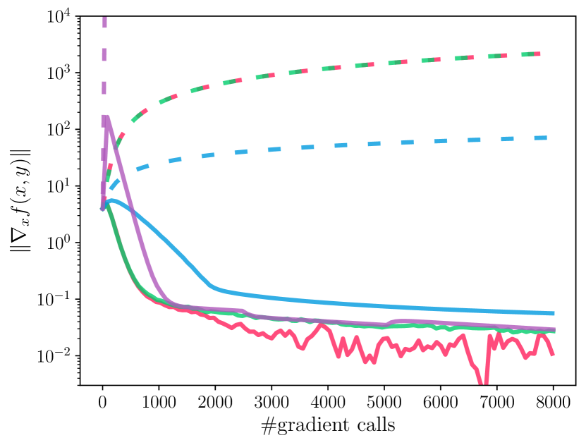
(a) $r=1$

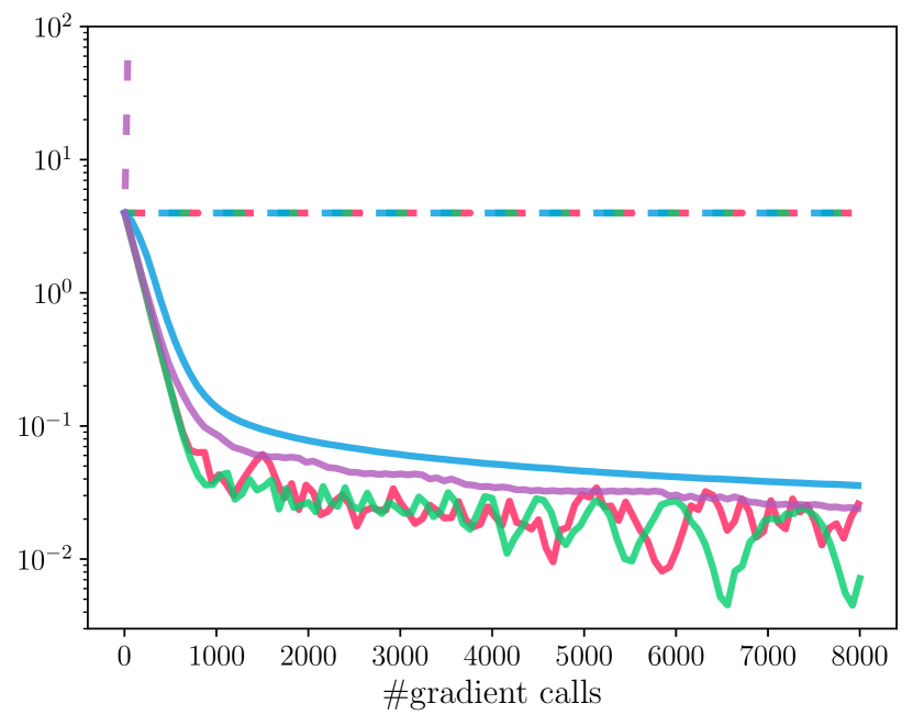
(b) $r=2$

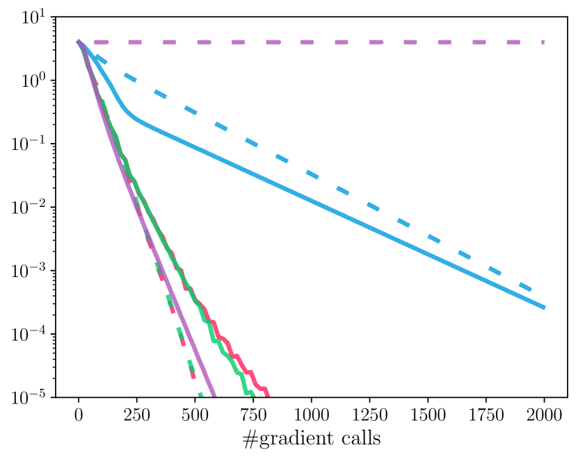
(c) $r=4$

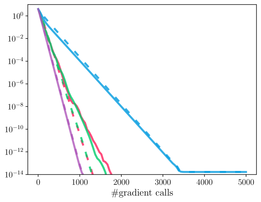
(d) $r=8$

Figure 1: Comparison between the two families of non-nested and nested adaptive methods on function $f(x,y)=-\frac{1}{2}y^{2}+2xy-2x^{2}$ with deterministic gradient oracles. $r=\eta^{y}/\eta^{x}$ is a pre-fixed learning rate ratio.

In this paper, we address these questions and make the following key contributions:

• We investigate two generic frameworks for adaptive minimax optimization: one is a simple (non-nested) adaptive framework, which performs one step of update of $x$ and $y$ simultaneously with adaptive gradients; the other is Nested Adaptive (NeAda) framework, which performs multiple updates of $y$ after one update of $x$, each with adaptive gradients. Both frameworks allow flexible choices of adaptive mechanisms such as Adam, AMSGrad and AdaGrad. We provide an example proving that the simple adaptive framework can fail to converge without setting an appropriate stepsize ratio; this applies to any of the adaptive mechanisms mentioned above, even in the noiseless setting. In contrast, the NeAda framework is less sensitive to the stepsize ratio, as numerically illustrated in Figure 1.

• We provide the convergence analysis for a representative of NeAda that uses AdaGrad stepsizes for $x$ and a convergent adaptive optimizer for $y$, in terms of nonconvex-strongly-concave minimax problems. Notably, the convergence of this general scheme does not require to know any problem parameters and does not assume the bounded gradients. We demonstrate that NeAda is able to achieve $\widetilde{O}(\epsilon^{-2})$ oracle complexity for the deterministic setting and $\widetilde{O}(\epsilon^{-4})$ for the stochastic setting to converge to $\epsilon$-stationary point, matching best known bounds. To the best of our knowledge, this seems to be the first adaptive framework for nonconvex minimax optimization that is provably convergent and parameter-agnostic.

• We further make two complementary contributions, which can be of independent interest. First, we propose a general AdaGrad-type stepsize for strongly-convex problems without knowing the strong convexity parameters, and derive a convergence rate comparable to SGD. It can serve as a subroutine for NeAda. Second, we provide a high probability convergence result for the primal variable of NeAda under a subGaussian assumption.

• Finally, we numerically validate the robustness of the NeAda framework on several test functions compared to the non-nested adaptive framework, and demonstrate the effectiveness of the NeAda framework on distributionally robust optimization task with a real dataset.

1.1 Related work

Adaptive algorithms.

Duchi et al. (2011) introduce AdaGrad for convex online learning and achieve $O(\sqrt{T})$ regrets. Li and Orabona (2019) and Ward et al. (2019) show an $\widetilde{O}(\epsilon^{-4})$ complexity for AdaGrad in the nonconvex stochastic optimization. There are an extensive number of works on AdaGrad-type methods; to list a few, (Levy et al., 2018; Antonakopoulos and Mertikopoulos, 2021; Kavis et al., 2019; Orabona and Pál, 2018). Another family of algorithms uses more aggressive stepsizes of exponential moving average of the past gradients, such as Adam (Kingma and Ba, 2015) and RMSProp (Hinton et al., 2012). Reddi et al. (2018) point out the non-convergence of Adam and provide a remedy with non-increasing stepsizes. There is a surge in the study of Adam-type algorithms due to their popularity in the deep neural network training (Zaheer et al., 2018; Chen et al., 2019; Liu et al., 2020a). Some work provides the convergence results for adaptive methods in the strongly-convex optimization (Wang et al., 2020; Levy, 2017; Mukkamala and Hein, 2017). Line search and stochastic line search are another effective strategy that can detect the objective’s curvature and have received much attention (Vaswani et al., 2019, 2021, 2020). Notably, many adaptive algorithms are parameter-agnostic (Duchi et al., 2011; Reddi et al., 2018; Ward et al., 2019).

Nonconvex minimax optimization.

Stationary convergence of GDA in NC-SC setting was first provided by Lin et al. (2020), showing $O(\epsilon^{-2})$ oracle complexity and $O(\epsilon^{-4})$ sample complexity with minibatch. Recently, Chen et al. (2021) and Yang et al. (2022) achieve this sample complexity in the stochastic setting without minibatch. GDmax is a double loop algorithm that maximizes the dual variable to a certain accuracy. It achieves nearly the same complexity as GDA (Nouiehed et al., 2019). Sebbouh et al. (2022) recently discuss the relation between the two-time-scale and number of inner steps for GDmax. Very recently, Li et al. (2022) provide the necessary and sufficient time-scale separation for GDA to converge locally to Stackelberg equilibrium. Besides NC-SC setting, some work provides convergent algorithms when the objective is (non-strongly) concave about the dual variable(Zhang et al., 2020; Lu et al., 2020; Yang et al., 2020b). Nonconvex-nonconcave regime is only explored under some special structure (Liu et al., 2021; Diakonikolas, 2020), such as Polyak-Łojasiewicz (PL) condition (Fiez et al., 2021; Yang et al., 2020a). All algorithms mentioned above require prior knowledge about problem parameters, such as smoothness modulus, strong concavity modulus, and noise variance.

Adaptive algorithms in minimax optimization.

There exist many adaptive and parameter-agnostic methods designed for convex-concave minimax optimization as a special case of monotone variational inequality (Bach and Levy, 2019; Antonakopoulos et al., 2019; Antonakopoulos, 2021; Ene and Nguyen, 2020; Stonyakin et al., 2018; Gasnikov et al., 2019; Malitsky, 2020; Diakonikolas, 2020). Most of them combine extragradient method, mirror prox (Nemirovski, 2004) or the like, with AdaGrad mechanism. Liu et al. (2020b) and Dou and Li (2021) relax convexity-concavity assumption to the regime where Minty variational inequality (MVI) has a solution. In these settings, time-scale separation of learning rates is not required even for non-adaptive algorithms. For nonconvex-strongly-concave problems, Huang and Huang (2021); Huang et al. (2021); Guo et al. (2021) propose adaptive methods, which set the learning rates based on knowledge about smoothness and strong-concavity modulus and the bounds for adaptive stepsizes.

2 Non-nested and nested adaptive methods

In this section, we investigate two generic frameworks that can incorporate most existing adaptive methods into minimax optimization. We remark that many variants encapsulated in these two families are already widely used in practice, such as training of GAN (Goodfellow, 2016), distributionally robust optimization (Sinha et al., 2018), etc. These two frameworks, coined as non-nested and nested adaptive methods, can be viewed as adaptive counterparts of GDA and GDmax. We aim to illustrate the difference between these two adaptive families, even though GDA and GDmax are often considered “twins”.

Non-nested adaptive methods.

In Algorithm 1, non-nested methods update the primal and dual variables in a symmetric way. Weighted gradients $m_{t}^{x}$ and $m_{t}^{y}$ are the moving average of the past stochastic gradients with the momentum parameters $\beta^{x}$ and $\beta^{y}$. The effective stepsizes of $x$ and $y$ are $\eta^{x}/\sqrt{v_{t}^{x}}$ and $\eta^{y}/\sqrt{v_{t}^{y}}$, where the division is taken coordinate-wise. We refer to $\eta^{x}$ and $\eta^{y}$ as learning rates, and $v_{t}^{x},v_{t}^{y}$ are some average of squared-past gradients through function $\psi$. Many popular choices of adaptive stepsizes are captured in this framework, see also (Reddi et al., 2018):

$$\text{(GDA)}\quad\beta=0;\ \ \psi\left(v_{0},\{g^{2}_{i}\}_{i=0}^{t}\right)=1,\quad\text{(AdaGrad)}\quad\beta=0;\ \ \psi\left(v_{0},\{g^{2}_{i}\}_{i=0}^{t}\right)=v_{0}+\sum_{i=0}^{t}g_{i}^{2},$$

$$\text{(Adam)}\quad\psi\left(v_{0},\{g^{2}_{i}\}_{i=0}^{t}\right)=\gamma^{t+1}v_{0}+(1-\gamma)\sum_{i=0}^{t}\gamma^{t-i}g_{i}^{2},$$

$$\text{(AMSGrad)}\quad\psi\left(v_{0},\{g^{2}_{i}\}_{i=0}^{t}\right)=\max_{m=0,\dots,t}\gamma^{m+1}v_{0}+(1-\gamma)\sum_{i=0}^{m}\gamma^{m-i}g_{i}^{2}.$$

Algorithm 1 Non-nested Adaptive Method

1:  Input: $x_{0}$ and $y_{0}$

2:  for $t=0,1,2,...$ do

3:     sample $\xi_{t}$ and let $g_{t}^{x}=\nabla_{x}F(x_{t},y_{t};\xi_{t})$ and $g_{t}^{y}=\nabla_{y}F(x_{t},y_{t};\xi_{t})$

4:     // update the first moment $m_{t+1}^{x}=\beta^{x}m^{x}_{t}+(1-\beta^{x})g_{t}^{x}$ and $m_{t+1}^{y}=\beta^{y}m^{y}_{t}+(1-\beta^{y})g_{t}^{y}$

5:     // update the second moment $v_{t+1}^{x}=\psi\left(v_{0}^{x},\{(g_{i}^{x})^{2}\}_{i=0}^{t}\right)$ and $v_{t+1}^{y}=\psi\left(v_{0}^{y},\{(g_{i}^{y})^{2}\}_{i=0}^{t}\right)$

6:     // update variables $x_{t+1}=x_{t}-\frac{\eta^{x}}{\sqrt{v_{t+1}^{x}}}m_{t+1}^{x}$ and $y_{t+1}=y_{t}+\frac{\eta^{y}}{\sqrt{v_{t+1}^{y}}}m_{t+1}^{y}$

7:  end for

Algorithm 2 Nested Adaptive (NeAda) Method

1:  Input: $x_{0}$ and $y_{0}^{0}$

2:  for $t=0,1,2,...$ do

3:     for $k=0,1,2,...$ until a stopping criterion is satisfied do

4:        sample $\hat{\xi}_{t}^{k}$ and $g_{t,k}^{y}=\nabla_{y}F(x_{t},y_{t}^{k};\hat{\xi}_{t}^{k})$

5:        $m_{t,k+1}^{y}=\beta^{y}m^{y}_{t,k}+(1-\beta^{y})g_{t,k}^{y}$

6:        $v_{t,k+1}^{y}=\psi^{y}\left(v_{t,0}^{y},\{(g_{t,i}^{y})^{2}\}_{i=0}^{k}\right)$

7:        $y_{t}^{k+1}=y_{t}^{k}+\frac{\eta^{y}}{\sqrt{v_{t,k+1}^{y}}}m_{t,k+1}^{y}$

8:     end for

9:     $v_{t+1,0}^{y}=v_{t,k+1}^{y}$ and $m_{t+1,0}^{y}=m^{y}_{t,k+1}$

10:     sample $\xi_{t}$ and $g_{t}^{x}=\nabla_{x}F(x_{t},y_{t}^{k+1};\xi_{t})$

11:     $m_{t+1}^{x}=\beta^{x}m^{x}_{t}+(1-\beta^{x})g_{t}^{x}$

12:     $v_{t+1}^{x}=\psi^{x}\left(v_{0}^{x},\{(g_{i}^{x})^{2}\}_{i=0}^{t}\right)$

13:     $x_{t+1}=x_{t}-\frac{\eta^{x}}{\sqrt{v_{t+1}^{x}}}m_{t+1}^{x}$

14:  end for

Nested adaptive (NeAda) methods.

NeAda, presented in Algorithm 2, has a nesting inner loop to maximize $y$ until some stopping criterion is reached (see details in Section 3). Instead of using a fixed number of inner iterations or a fixed target accuracy as in GDmax (Lin et al., 2020; Nouiehed et al., 2019), NeAda gradually increases the accuracy of the inner loop as the outer loop proceeds to make it fully adaptive.

We refer to the ratio between two learning rates, i.e. $\eta^{y}/\eta^{x}$, as the two-time-scale. The current analysis of GDA in nonconvex-strongly-concave setting requires two-time-scale to be proportional with the condition number $\kappa=l/\mu$, where $l$ and $\mu$ are Lipschitz smoothness and strongly-concavity modulus (Lin et al., 2020; Yang et al., 2022). We provide an example showing that the problem-dependent two-time-scale is necessary for GDA and most non-nested methods even in the deterministic setting.

Lemma 2.1.

Consider the function $f(x,y)=-\frac{1}{2}y^{2}+Lxy-\frac{L^{2}}{2}x^{2}$ in the deterministic setting. Let $r\eta^{x}=\eta^{y}$. (1) GDA will not converge to the stationary point when $r\leq L^{2}$:

$$\nabla_{x}f(x_{T},y_{T})=\nabla_{x}f(x_{0},y_{0})\prod_{t=0}^{T-1}\left[1+\eta^{x}(L^{2}-r)\right].$$

(2) Assume the averaging function $\psi^{x}$ and $\psi^{y}$ are the same, and satisfy that for any $\tau$, if $v_{t}^{x}=\tau v_{t}^{y}$ and $(g_{t}^{x})^{2}=\tau(g_{t}^{y})^{2}$ then $v_{t+1}^{x}=\tau v_{t+1}^{y}$. With $\beta^{x}=\beta^{y}$, $v_{0}^{x}=v_{0}^{y}=0$ and $m_{0}^{x}=m_{0}^{y}=0$ (which are commonly used in practice), non-nested adaptive method will not converge when $r\leq L$:

$$\nabla_{x}f(x_{T},y_{T})\geq\nabla_{x}f(x_{0},y_{0})\prod_{t=0}^{T-1}\left[1+\frac{L\eta^{x}}{\sqrt{v_{t}^{x}}}(1-\beta^{x})(L-r)\right].$$

When $r=L$, $\nabla_{x}f(x_{t},y_{t})=\nabla_{x}f(x_{0},y_{0})$ for all $t$.

Remark 1.

Most popular adaptive stepsizes we mentioned before, such as Adam, AMSGrad and AdaGrad, have averaging functions satisfying the assumption in the lemma. Any point on the line $y=Lx$ is a stationary point for the above function, and the distance from a point to this line is proportional to its gradient norm, so the divergence in gradient norm will also implies that of iterates. In the proof, we will also show that the averaged or best iterate will still diverge under the same condition. The lemma implies that for any given time-scale $r$, there exists a problem for which the non-nested algorithm does not converge to the stationary point, so they are not parameter-agnostic.

We compare non-nested and nested methods combined with different stepsizes schemes: Adam, AMSGrad, AdaGrad and fixed stepsize, on the function: $-\frac{1}{2}y^{2}+2xy-2x^{2}$. In the experiments of this section, we halt the inner loop when the (stochastic) gradient about $y$ is smaller than $1/t$ or the number iteration is greater than $t$. We observe from Figure 1 that the thresholds for the non-convergence of non-nested methods ($r=2$ for adaptive methods and $r=4$ for GDA) are exactly as predicted by the lemma. Although the adaptive methods admit a smaller two-time-scale threshold than GDA in this example, it is not a universal phenomenon from our experiments in Section 4. Interestingly, nested adaptive methods are robust to different two-time-scales and always have the trend to converge to the stationary point.

3 Convergence Analysis of NeAda-AdaGrad

In this section, we reveal the secret behind the robust performance of NeAda by providing the convergence guarantee for a representative member in the family. For sake of simplicity and clarity, we mainly focus on NeAda with AdaGrad. Adam-type mechanism can suffer from non-convergence already for nonconvex minimization despite its good performance in practice. Our result also sheds light on the analysis of other more sophisticated members such as AMSGrad in the family.

NeAda-AdaGrad:

Presented in Algorithm 3, NeAda-AdaGrad adopts the scalar AdaGrad scheme for the $x$-update in the outer loop and uses mini-batch in the stochastic setting. For the inner loop for maximizing $y$, we run some adaptive algorithm for maximizing $y$ until some easily checkable stopping criterion is satisfied. We suggest two criteria here: at $t$-th outer loop: (I) the squard gradient mapping norm about $y$ is smaller than $1/(t+1)$ in the deterministic setting, (II) the number of inner loop iterations reaches $t+1$ in the stochastic setting.

Algorithm 3 NeAda-AdaGrad

1:  Input: $(x_{0},y_{-1})$, $v_{0}>0$, $\eta>0$.

2:  for $t=0,1,2,...,T-1$ do

3:     from $y_{t-1}$ run an adaptive algorithm $\mathcal{A}$ for maximizing $f(x_{t},\cdot)$ to obtain $y_{t}$ (a) stopping criterion I (deterministic): stop when $\|y_{t}-\text{Proj}_{\mathcal{Y}}(y_{t}+\nabla_{y}f(x_{t},y_{t}))\|^{2}\leq\frac{1}{t+1}$ (b) stopping criterion II (stochastic): stop after $t+1$ inner loop iterations.

4:     $v_{t+1}=v_{t}+\left\|\frac{1}{M}\sum_{i=1}^{M}\nabla_{x}F(x_{t},y_{t};\xi^{i}_{t})\right\|^{2}$ where $\{\xi^{i}_{t}\}_{i=1}^{M}$ are i.i.d samples

5:     $x_{t+1}=x_{t}-\frac{\eta}{\sqrt{v_{t+1}}}\left(\frac{1}{M}\sum_{i=1}^{M}\nabla_{x}F(x_{t},y_{t};\xi^{i}_{t})\right)$

6:  end for

For the purpose of theoretical analysis, we mainly focus on the minimax problem of the form (1) under the nonconvex-strongly-concave (NC-SC) setting, formally stated in the following assumptions.

Assumption 3.1 (Lipschitz smoothness).

There exists a positive constant $l>0$ such that

$$\max\big{\{}\left\|\nabla_{x}f\left(x_{1},y_{1}\right)-\nabla_{x}f\left(x_{2},y_{2}\right)\right\|,\left\|\nabla_{y}f\left(x_{1},y_{1}\right)-\nabla_{y}f\left(x_{2},y_{2}\right)\right\|\big{\}}\leq l[\left\|x_{1}-x_{2}\right\|+\left\|y_{1}-y_{2}\right\|],$$

holds for all $x_{1},x_{2}\in\mathbb{R}^{d},y_{1}$, $y_{2}\in\mathcal{Y}$.

Assumption 3.2 (Strong-concavity in $y$).

There exists $\mu>0$ such that: $f(x,y_{1})\geq f(x,y_{2})+\langle\nabla_{y}f(x,y_{1}),y_{1}-y_{2}\rangle+\frac{\mu}{2}\|y_{1}-y_{2}\|^{2},\forall x\in\mathbb{R}^{d},y_{1},y_{2}\in\mathcal{Y}.$

For simplicity of notation, define $\kappa=l/\mu$ as the condition number, $\Phi(x)=\max_{y\in\mathcal{Y}}f(x,y)$ as the primal function, and $y^{*}(x)=\mathop{\rm argmax}_{\mathcal{Y}}f(x,y)$ as the optimal $y$ w.r.t $x$. Since the objective is nonconvex about $x$, we aim at finding an $\epsilon$-stationary point $(x_{t},y_{t})$ such that $\mathbb{E}\|\nabla_{x}f(x_{t},y_{t})\|\leq\epsilon$ and $\mathbb{E}\|y_{t}-y^{*}(x_{t})\|\leq\epsilon$, where the expectation is taken over the randomness in the algorithm.

3.1 Convergence in deterministic and stochastic settings

Assumption 3.3 (Stochastic gradients).

$\nabla_{x}F(x,y;\xi)$ and $\nabla_{y}F(x,y;\xi)$ are unbiased stochastic estimators of $\nabla_{x}f(x,y)$ and $\nabla_{y}f(x,y)$ and have variances bounded by $\sigma^{2}\geq 0$.

We assume the unbiased stochastic gradients have the variance $\sigma^{2}$, and the problem reduces to the deterministic setting when $\sigma=0$. Now we provide a general analysis of the convergence for any adaptive optimizer used in the inner loop.

Theorem 3.1.

Define the expected cumulative suboptimality of inner loops as $\mathcal{E}=\mathbb{E}\left[\sum_{t=0}^{T-1}\frac{l^{2}\|y_{t}-y^{*}(x_{t})\|^{2}}{2\sqrt{v_{0}}}\right]$. Under Assumptions 3.1, 3.2 and 3.3, the output from Algorithm 3 satisfies

$$\mathbb{E}\left[\sqrt{\frac{1}{T}\sum_{t=0}^{T-1}\|\nabla_{x}f(x_{t},y_{t})\|^{2}}\right]\leq\frac{2(A+\mathcal{E})}{\sqrt{T}}+\frac{v_{0}^{\frac{1}{4}}\sqrt{A+\mathcal{E}}}{\sqrt{T}}+\frac{2\sqrt{(A+\mathcal{E})\sigma}}{(MT)^{\frac{1}{4}}},$$

where $A=\frac{2\Delta}{\eta}+\left(\frac{4\sigma}{\sqrt{M}}+2\kappa l\eta\right)\left[1+2\log\left(\mathrm{Poly}\left(T,\mathcal{E},\frac{\Delta}{\eta},\frac{\sigma}{\sqrt{M}},\kappa l\eta,v_{0},\frac{1}{v_{0}}\right)\right)\right]$.

Remark 2.

The general analysis is built upon milder assumptions than existing work on AdaGrad in nonconvex optimization, not requiring either bounded gradient in (Ward et al., 2019) or prior knowledge about the smoothness modulus in (Li and Orabona, 2019). This theorem implies the algorithm attains convergence for the nonconvex variable $x$ with any constant $\eta>0$ and $v_{0}>0$ that does not depend on any problem parameter, so it is parameter-agnostic.

Remark 3.

Another benefit of this analysis is that the variance $\sigma$ appears in the leading term $T^{-\frac{1}{4}}$, which means the convergence rate can interpolate between the deterministic and stochastic settings. It implies a complexity of $\widetilde{O}(\epsilon^{-2})$ in the deterministic setting and $\widetilde{O}(\epsilon^{-4})$ in the stochastic setting for the primal variable as long as the accumulated suboptimality for the inner-loops $\mathcal{E}$ is $\widetilde{\mathcal{O}}(1)$, regardless of the batch size $M$. However, $M$ can control the number of outer loops and there affect the sample complexity for the dual variable.

In the next two theorems, we derive the total complexities, in the deterministic and stochastic settings, of finding $\epsilon$-stationary point by controlling the cumulative suboptimality $\mathcal{E}$ in Theorem 3.1 for subroutine $\mathcal{A}$ with specific convergence rate. In fact, we can also use any off-the-shelf adaptive optimizer for solving the inner maximization problem up to the desired accuracy. Note that (stochastic) GDmax fixes each inner-loop’s accuracy or steps to be related with $\mu$, $\ell$ and $\epsilon$ so that $\mathcal{E}$ can be easily bounded (Lin et al., 2020; Nouiehed et al., 2019). In contrast, since we do not have access to the problem parameters and $\epsilon$, Algorithm 3 gradually increases the inner-loop accuracy. In the proof of the following theorems, we will show that with our proposed stopping criteria and desired subroutines, $\mathcal{E}$ is bounded by $\mathcal{O}(\log T)$.

Theorem 3.2 (deterministic).

Suppose we have a linearly-convergent subroutine $\mathcal{A}$ for maximizing any strongly concave function $h(\cdot)$:

$$\|y^{k}-y^{*}\|^{2}\leq a_{1}(1-a_{2})^{k}\|y^{0}-y^{*}\|^{2}$$

where $y^{k}$ is $k$-th iterate, $y^{*}$ is the optimal solution, and $a_{1}>0$ and $0<a_{2}<1$ are constants that can depend on the parameters of $h$. Under the same setting as Theorem 3.1 with $\sigma=0$, for Algorithm 3 with $M=1$ and a subroutine $\mathcal{A}$ under stopping criterion I, there exists $t^{*}\leq\widetilde{O}\left(\epsilon^{-2}\right)$ such that $(x_{t^{*}},y_{t^{*}})$ is an $\epsilon$-stationary point. Therefore, the total gradient complexity is $\widetilde{O}\left(\epsilon^{-2}\right)$.

Remark 4.

This complexity is optimal in $\epsilon$ up to logarithmic term (Zhang et al., 2021), similar to GDA (Lin et al., 2020). Note that many adaptive and parameter-agnostic algorithms can achieve the linear rate when solving smooth and strongly concave maximization problems; to list a few, gradient ascent with backtracking line-search (Vaswani et al., 2019), SC-AdaNGD (Levy, 2017) and polyak stepsize (Hazan and Kakade, 2019; Loizou et al., 2021; Orvieto et al., 2022) . Here we can also pick more general subproblem accuracy in criterion I that only needs to scale with $1/t$.

Theorem 3.3 (stochastic).

Suppose we have a sub-linearly-convergent subroutine $\mathcal{A}$ for maximizing any strongly concave function $h(\cdot)$: after $K=k+1$ iterations

$$\mathbb{E}\|y^{K}-y^{*}\|^{2}\leq\frac{b_{1}\|y^{0}-y^{*}\|^{2}+b_{2}}{k},$$

where $y^{k}$ is $k$-th iterate, $y^{*}$ is the optimal solution, and $b_{1},b_{2}>0$ are constants that can depend on the parameters of $h$. Under the same setting as Theorem 3.1, for Algorithm 3 with $M=\epsilon^{-2}$ and subroutine $\mathcal{A}$ under the stopping criterion II, there exists $t^{*}\leq\widetilde{O}\left(\epsilon^{-2}\right)$ such that $(x_{t^{*}},y_{t^{*}})$ is an $\epsilon$-stationary point. Therefore, the total stochastic gradient complexity is $\widetilde{O}\left(\epsilon^{-4}\right).$

Remark 5.

This $\widetilde{O}\left(\epsilon^{-4}\right)$ complexity is nearly optimal in the dependence of $\epsilon$ for stochastic NC-SC problems (Li et al., 2021). Here we set $M=\epsilon^{-2}$ for the simplicity of exposition, and a similar result also holds for gradually increasing $M$. The sublinear rate specified above for solving the stochastic strongly convex subproblem can be achieved by several existing parameter-agnostic algorithms under some additional assumptions, such as FreeRexMomentum (Cutkosky and Boahen, 2017) and Coin-Betting (Cutkosky and Orabona, 2018). Parameter-free SGD (Carmon and Hinder, 2022) is partially parameter-agnostic that only requires the stochastic gradient bound rather than the strongly-convexity parameter. Mukkamala and Hein (2017) and Wang et al. (2020) introduce the variants of AdaGrad, RMSProp and Adam for strongly-convex online learning, but they need to know both gradient bounds and strongly-convexity parameter for setting stepsizes. We will show in the next subsection that AdaGrad with a slower decaying rate is parameter-agnostic. We note that the analysis of this theorem is not the simple gluing of the outer loop and inner loop complexity, but requires more sophisticated control of the cumulative suboptimality $\mathcal{E}$.

With the popularity of computational resource demanding deep neural networks, in both minimization and minimax applications, people find high probability guarantees for a single run of an algorithm useful (Kavis et al., 2022; Li and Orabona, 2020). Given the lack of such guarantee in the minimax optimization, we provide a high probability convergence result for NeAda-AdaGrad in Appendix C, which shows a similar sample complexity as Theorem 3.3 under the subGaussian noise.

3.2 Generalized AdaGrad for strongly-convex subproblem

We now introduce the generalized AdaGrad for minimizing strongly convex objectives, which can serve as an adaptive subroutine for Algorithm 3, without requiring knowledge on the strongly convex parameter. We analyze it for the more general online convex optimization setting: at each round $t$, the learner updates its decision $x_{t}$, then it suffers a loss $f_{t}(x_{t})$ and receives the sub-gradient of $f_{t}$. The generalized AdaGrad, described in Algorithm 4, keeps the cumulative gradient norm $v_{t}$ and takes the stepsize $\eta/v_{t}^{\alpha}$ with a decaying rate $\alpha\in(0,1]$. When $\alpha=1/2$, it reduces to the scalar version of the original AdaGrad (Duchi et al., 2011); when $\alpha=1$, it reduced to the scalar version of SC-AdaGrad (Mukkamala and Hein, 2017).

Algorithm 4 Generalized AdaGrad for Strongly-convex Online Learning

1:  Input: $x_{0}$, $v_{0}>0$ and $0<\alpha\leq 1$ .

2:  for $t=0,1,2,...$ do

3:     receive $g_{t}\in\partial f_{t}(x_{t})$

4:     $v_{t+1}=v_{t}+\|g_{t}\|^{2}$

5:     $x_{t+1}=\mathcal{P}_{\mathcal{X}}\left(x_{t}-\frac{\eta}{v_{t+1}^{\alpha}}g_{t}\right)$

6:  end for

Theorem 3.4.

Consider Algorithm 4 for online convex optimization and assume that (i) $f_{t}$ is continuous and $\mu$-strongly convex, (ii) $\mathcal{X}$ is convex and compact with diameter $\mathcal{D}$; (iii) $\|g_{t}\|\leq G$ for every $t$. Then for $0<\alpha<1$ with any $\eta>0$, the regret of Algorithm 4 satisfies:

$$\max_{x\in\mathcal{X}}\sum_{t=0}^{T-1}(f_{t}(x_{t})-f_{t}(x))\leq c_{\alpha}+d_{\alpha}\left(v_{0}+\sum_{t=1}^{T-1}\|g_{t}\|^{2}\right)^{1-\alpha},$$

and for $\alpha=1$ with $\eta\geq\frac{G^{2}}{2\mu}$,

$$\max_{x\in\mathcal{X}}\sum_{t=0}^{T-1}(f_{t}(x_{t})-f_{t}(x))\leq c_{\alpha}+d_{\alpha}\log\left(v_{0}+\sum_{t=1}^{T-1}\|g_{t}\|^{2}\right),$$

where $c_{\alpha}$ and $d_{\alpha}$ are constants depending on the problem parameters, $\alpha$ and $\eta$.

The theorem implies a logarithmic regret for the case $\alpha=1$, but the stepsize needs knowledge about problem’s parameters $\mu$ and $G$; similar results are shown for SC-AdaGrad (Mukkamala and Hein, 2017) and SAdam (Wang et al., 2020). When $\alpha<1$, the algorithm becomes parameter-agnostic and attains an $O(T^{1-\alpha})$ regret. Such parameter-agnostic phenomenon for smaller decaying rates is also observed for SGD in stochastic optimization (Fontaine et al., 2021). Proving the regret bound for the generalized AdaGrad with $\alpha<1$ in the online setting is challenging, since the adversarial $g_{t}$ can lead to a “sudden” change in the stepsize. In the proof, we bound the possible number of times such “sudden” change could happen.

To the best of our knowledge, this is the first regret bound for adaptive methods with general decaying rates in the strongly convex setting. By online-to-batch conversion (Kakade and Tewari, 2008), it can be converted to $O(T^{-\alpha})$ rate in the strongly convex stochastic optimization. Xie et al. (2020) prove the $O(1/T)$ convergence rate, or a linear convergence rate when the smoothness parameter is known, for AdaGrad with $\alpha=1/2$ in this setting, but under a strong assumption — Restricted Uniform Inequality of Gradients (RUIG) — that requires the loss function with respect to each sample $\xi$ to satisfy the error bound condition with some probability.

4 Experiments

To evaluate the performance of NeAda, we conducted experiments on simple test functions and a real-world application of distributional robustness optimization (DRO). In all cases, we compare NeAda with the non-nested adaptive methods using the same adaptive schemes. For notational simplicity, in all figure legends, we label the non-nested methods with the names of the adaptive mechanisms used. We observe from all our experiments that: 1) while non-nested adaptive methods can diverge without the proper two-time-scale, NeAda with adaptive subroutine always converges; 2) when the non-nested method converges, NeAda can achieve comparable or even better performance.

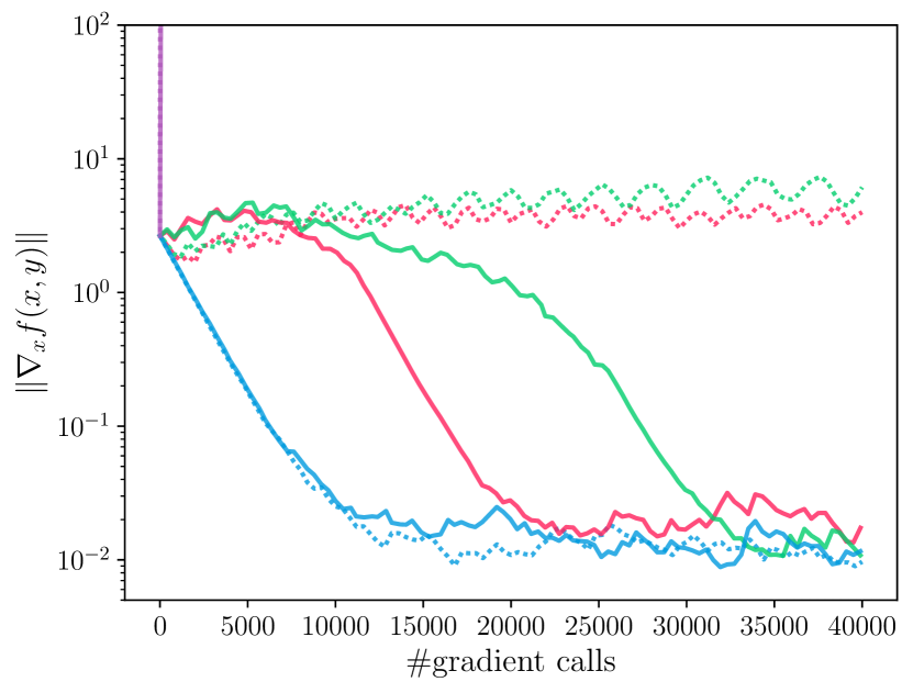
(a) $r=0.01$

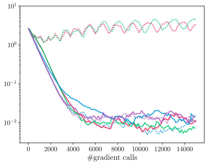
(b) $r=0.03$

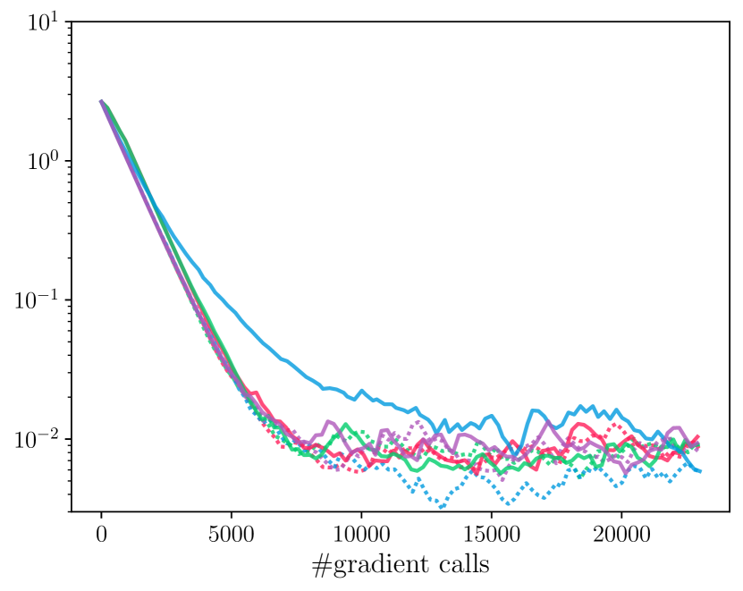
(c) $r=0.05$

Figure 2: Comparison between the two families of non-nested and nested adaptive methods on McCromick function with stochastic gradient oracles. $\sigma=0.01$, $\eta^{y}=0.01$ and $r=\eta^{y}/\eta^{x}$.

4.1 Test functions

In Section 2, we have compared NeAda with non-nested methods on a quadratic function in Figure 1 and the observations match Lemma 2.1. Now we consider a more complicated function that is composed of McCormick function in $x$, a bilinear term, and a quadratic term in $y$,

$$f(x,y)=\sin(x_{1}+x_{2})+(x_{1}-x_{2})^{2}-\frac{3}{2}x_{1}+\frac{5}{2}x_{2}+1+x_{1}y_{1}+x_{2}y_{2}-\frac{1}{2}(y_{1}^{2}+y_{2}^{2}),$$

For this function, we compare the adaptive frameworks in the stochastic setting with Gaussian noise. As demonstrated in Figure 2, non-nested methods are sensitive to the selection of the two-time-scale. When the learning rate ratio is too small, e.g., $\eta^{y}/\eta^{x}=0.01$, non-nested Adam, AMSGrad and GDA all fail to converge. We observe that GDA converges when the ratio reaches 0.03, while non-nested Adam and AMSGrad still diverge until 0.05. Although non-nested adaptive methods require a smaller ratio than GDA in Lemma 2.1, this example illustrates that adaptive algorithms sometimes can be more sensitive to the time separation. In comparison, NeAda with adaptive subroutine always converges regardless of the learning rate ratio.

4.2 Distributional robustness optimization

To justify the effectiveness of NeAda on real-world applications, we carried out experiments on distributionally robust optimization (Sinha et al., 2018), where the primal variable is the model weights to be learned by minimizing the empirical loss while the dual variable is the adversarial perturbed inputs. The dual variable problem targets finding perturbations that maximize the empirical loss but not far away from the original inputs. Formally, for model weights $x$ and adversarial samples $y$, we have:

$$\min_{x}\max_{y=[y_{1},\dots,y_{n}]}f(x,y),\quad\text{where}\quad f(x,y)\coloneqq\frac{1}{n}\sum_{i=1}^{n}f_{i}(x,y_{i})-\gamma\left\|y_{i}-v_{i}\right\|^{2},$$

where $n$ is the total number of training samples, $v_{i}$ is the $i$-th original input and $f_{i}$ is the loss function for the $i$-th sample. $\gamma$ is a trade-off parameter between the empirical loss and the magnitude of perturbations. When $\gamma$ is large enough, this problem is nonconvex-strongly-concave, and following the same setting as (Sinha et al., 2018; Sebbouh et al., 2022), we set $\gamma=1.3$. For NeAda, we use both stopping criterion I with stochastic gradient and criterion II in our experiments. For the results, we report the training loss and the test accuracy on adversarial samples generated from fast gradient sign method (FGSM) (Goodfellow et al., 2014b). FGSM can be formulated as

$$x_{\text{adv}}=x+\epsilon\cdot\text{sign}\left(\nabla_{x}f(x)\right),$$

where $\epsilon$ is the noise level. To get reasonable test accuracy, NeAda with Adam as subroutine is compared with Adam with fixed 15 inner loop iterations, which is consistent with the choice of inner loop steps in (Sinha et al., 2018), and such choice obtains much better test accuracy than the completely non-nested Adam. Our experiments include a synthetic dataset and MNIST (LeCun, 1998) with code modified from (Lv, 2019).

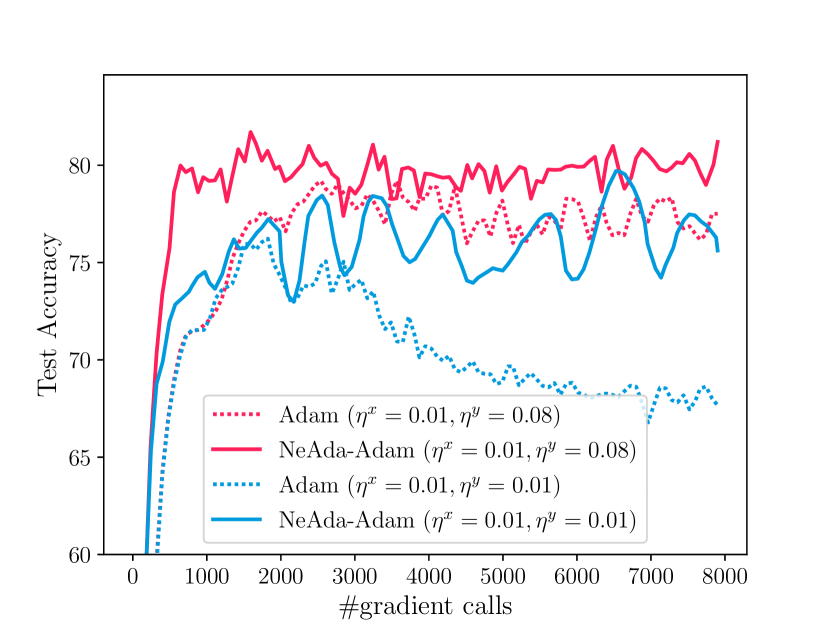
(a) Test Accuracy

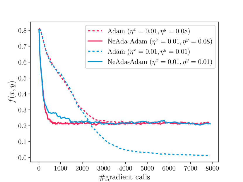
(b) Training Loss

Figure 3: Experimental results of distributional robustness optimization task on synthetic dataset.

Results on Synthetic Dataset.

We use the same data generation process as in (Sinha et al., 2018). The inputs are 2-dimensional i.i.d. random Guassian vectors, i.e., $x_{i}\sim\mathcal{N}(0,I_{2})$, where $I_{2}$ is the $2\times 2$ identity matrix. The corresponding $y_{i}$ is defined as $y_{i}=\text{sign}(\left\|x_{i}\right\|_{2}-\sqrt{2})$. Data points with norm in range $(\sqrt{2}/1.3,1.3\sqrt{2})$ are removed to make the classification margin wide. $10000$ training and $4000$ test data points are generated for our experiments. The model we use is a three-layer MLP with ELU activations.

As shown in Figure 3(a), when the learning rates are set to different scales, i.e., $\eta^{x}=0.01,\eta^{y}=0.08$ (red curves in the figure), both methods achieve reasonable test errors. In this case, NeAda has higher test accuracy and reaches such accuracy faster than Adam. If we change the learning rates to the same scale, i.e., $\eta^{x}=0.01,\eta^{y}=0.01$ (blue curves in the figure), NeAda retains good accuracy while Adam drops to an unsatisfactory performance. This demonstrates the adaptivity and less-sensitivity to learning rates of NeAda. In addition, Figure 3(b) illustrates the convergence speeds on the loss function, and NeAda (solid lines) always decreases the loss faster than Adam. Note that Adam with the same learning rates converges to a lower loss but suffers from overfitting, as shown in Figure 3(a) that its test accuracy is only about 68%.

Results on MNIST Dataset.

For MNIST, we use a convolutional neural network with three convolutional layers and one final fully-connected layer. Following each convolutional layer, ELU activation and batch normalization are used.

We compare NeAda with Adam under three different noise levels and the accuracy is shown in Figures 4(a), 4(b) and 4(c). Under all noise levels, NeAda outperforms Adam with the same learning rates. When we have proper time-scale separation (the red curves), both methods achieve good test accuracy, and NeAda achieves higher accuracy and converges faster. After we change to the same learning rates for the primal and dual variables (the blue curves), the accuracy drop of NeAda is slighter compared to Adam, especially when $\epsilon=0.1$. As for the training loss shown in Figure 4(d), NeAda (the solid curves) is always faster at the beginning. We also observed that with proper time-scale separation, NeAda reaches a lower loss.

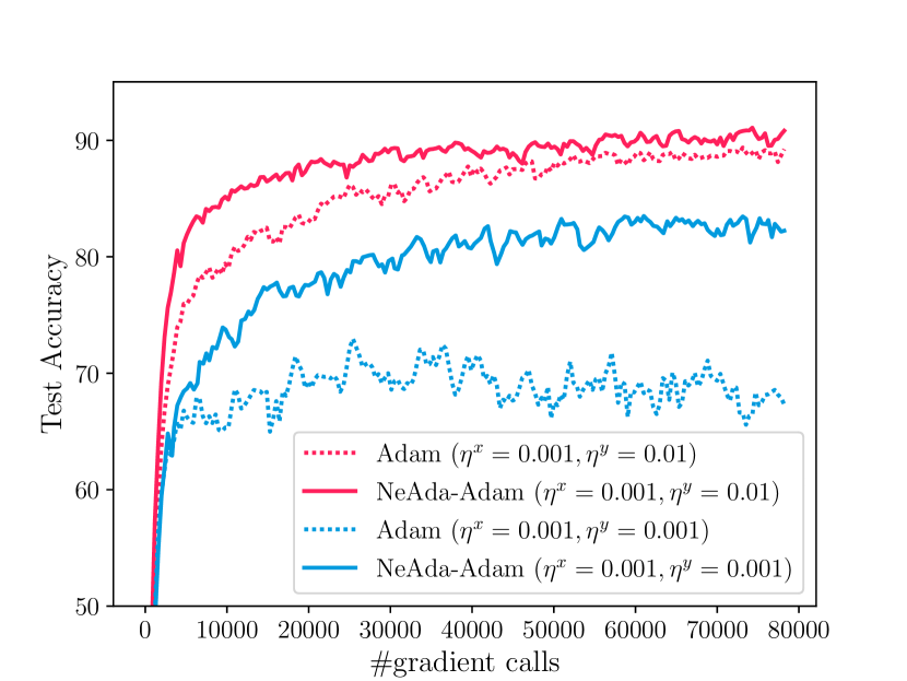
(a) $\epsilon=0.1$

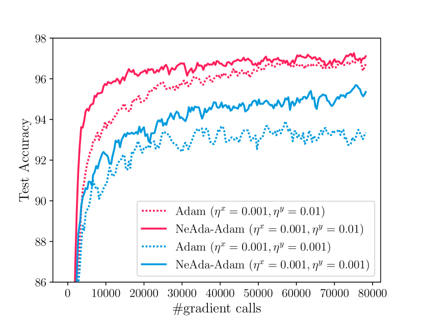
(b) $\epsilon=0.05$

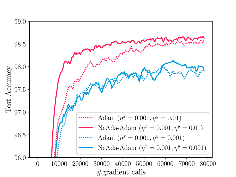
(c) $\epsilon=0.02$

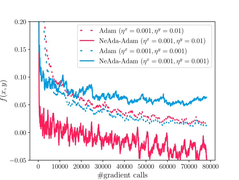
(d) loss

Figure 4: Results of distributional robustness optimization task on MNIST. $\epsilon$ is the noise level.

5 Conclusion

Both non-nested and nested adaptive methods are popular in nonconvex minimax problems, e.g., the training of GANs. In this paper, we demonstrate that non-nested algorithms may fail to converge when the time-scale separation is ignorant of the problem parameter even when the objective is strongly-concave in the dual variable with noiseless gradients information. We propose fixes to this problem with a family of nested algorithms–NeAda, that nests the max oracle of the dual variable under an inner loop stopping criterion. The proper stopping criterion will help to balance the outer loop progress and inner loop accuracy. NeAda-AdaGrad attains the near-optimal complexity without a priori knowledge of problem parameters in the nonconvex-strongly-concave setting. It can be a future direction to design parameter-agnostic algorithms for nonconvex-concave minimax problems or more general regimes by leveraging recent progress in nonconvex minimax optimization and the adaptive analysis in this paper. Another interesting direction is to investigate the convergence behavior of Adam-type algorithms with general decaying rates in the strongly convex online optimization.

Appendix A Helper Lemmas and Proofs for Section 2

A.1 Helper Lemmas

Lemma A.1 (Lemma 4.3 in (Lin et al., 2020) and Lemma A.5 in (Nouiehed et al., 2019)).

Under Assumptions 3.1 and 3.2, define $\Phi(x)=\max_{y\in\mathcal{Y}}f(x,y)$. Define $y^{*}(x)=\mathop{\rm argmax}_{y\in\mathcal{Y}}f(x,y)$. Then $y^{*}(\cdot)$ is $\kappa$-Lipschitz with $\kappa=\frac{l}{\mu}$, $\Phi(\cdot)$ is L-smooth with $L:=l+l\kappa$ and $\nabla\Phi(x)=\nabla_{x}f\left(x,y^{*}(x)\right)$.

Lemma A.2.

Let $x_{1},...,x_{T}$ be a sequence of non-negative real numbers, $x_{1}>0$ and $0<\alpha<1$. Then we have

$$\left(\sum_{t=1}^{T}x_{t}\right)^{1-\alpha}\leq\sum_{t=1}^{T}\frac{x_{t}}{\left(\sum_{k=1}^{t}x_{k}\right)^{\alpha}}\leq\frac{1}{1-\alpha}\left(\sum_{t=1}^{T}x_{t}\right)^{1-\alpha}.$$

When $\alpha=1$, we have

$$\sum_{t=1}^{T}\frac{x_{t}}{\left(\sum_{k=1}^{t}x_{k}\right)^{\alpha}}\leq 1+\log\left(\frac{\sum_{t=1}^{t}x_{t}}{x_{1}}\right).$$

Remark 6.

The case $\alpha=1/2$ has been noticed in (Auer et al., 2002), and the upper bound in the case $\alpha=1$ has already been noticed in (Ward et al., 2019). Here we we extend it to $0<\alpha\leq 1$.

• For the first inequality, we have

  $$\sum_{t=1}^{T}\frac{x_{t}}{\left(\sum_{k=1}^{t}x_{k}\right)^{\alpha}}\geq\sum_{t=1}^{T}\frac{x_{t}}{\left(\sum_{k=1}^{T}x_{k}\right)^{\alpha}}=\frac{\sum_{t=1}^{T}x_{t}}{\left(\sum_{t=1}^{T}x_{t}\right)^{\alpha}}=\left(\sum_{t=1}^{T}x_{t}\right)^{1-\alpha}.$$

  For the second inequality, we follow a similar procedure as in the proof of Lemma 3.5 of (Auer et al., 2002). First consider the case $0<\alpha<1$. By Bernoulli’s inequality, as $y\leq 1$ and $0<\alpha<1$, we have $1-(1-\alpha)y\geq(1-y)^{1-\alpha}$. Denoting $S_{t}=\sum_{k=1}^{t}x_{k}$ and $S_{0}=0$, by replacing $y$ with $x_{t}/S_{t}$, we have

  $$(1-\alpha)\frac{x_{t}}{S_{t}}\leq 1-\left(1-\frac{x_{t}}{S_{t}}\right)^{1-\alpha}.$$

  Multiplying both sides by $S_{t}^{1-\alpha}$, then we have

  $$(1-\alpha)\frac{x_{t}}{S_{t}^{\alpha}}\leq S_{t}^{1-\alpha}-S_{t-1}^{1-\alpha}.$$

  Summing over the inequalities for $t=1,...,T$ gives us the desired result. For $\alpha=1$, it is proved by (Ward et al., 2019). ∎

Proposition A.1.

If $x^{2}\leq(a_{1}+a_{2}x)\left(a_{3}+a_{4}\log(a_{5}a_{1}+a_{5}a_{2}x)\right)$ with $x,a_{1},a_{2},a_{3},a_{4},a_{5}\geq 0$ and $a_{2}>0$, then

$$x\leq\frac{a_{1}}{a_{2}}+16a_{2}^{3}a_{4}^{2}a_{5}+3a_{2}^{2}a_{3}^{2}$$

• The proof is similar to Lemma 6 in (Li and Orabona, 2019). If $a_{2}x<a_{1}$, we have $x\leq a_{1}/a_{2}$. Assume $a_{2}x\geq a_{1}$, then

  $$x^{2}\leq 2a_{2}x(a_{3}+a_{4}\log(2a_{5}a_{2}x))\leq 2a_{2}x\left(a_{3}+a_{4}\sqrt{2a_{5}a_{2}x}\right),$$

  which implies

  $$x\leq 2a_{2}a_{3}+2a_{2}a_{4}\sqrt{2a_{5}a_{2}x}\quad\Longrightarrow\quad x^{2}\leq 8a_{2}^{2}a_{3}^{2}+16a_{2}^{3}a_{4}^{2}a_{5}x.$$

  Solving this, we get

  $$x\leq 8a_{2}^{3}a_{4}^{2}a_{5}+\sqrt{64a_{2}^{6}a_{4}^{4}a_{5}^{2}+8a_{2}^{4}a_{3}^{4}}\leq 16a_{2}^{3}a_{4}^{2}a_{5}+3a_{2}^{2}a_{3}^{2}.$$

∎

Proposition A.2.

Assume $x_{t},a_{t},b_{t}>0$, for $t=0,1,2,...$, and $x_{t+1}\leq a_{t}x_{t}+b_{t}$, then we have

$$x_{T}\leq\left(\prod_{t=0}^{T-1}a_{t}\right)x_{0}+\sum_{t=0}^{T-2}\left(\prod_{i=t+1}^{T-1}a_{i}\right)b_{t}+b_{T-1},\quad T\geq 2$$

• Let’s prove it by induction. It is obvious that this inequality holds for $T=2$:

  $$x_{2}=a_{1}x_{1}+b_{1}=a_{1}a_{0}x_{0}+a_{1}b_{0}+b_{1}.$$

  Assume this inequality holds for $T$, then

  $$x_{T+1}\leq a_{T}\left[\left(\prod_{t=0}^{T-1}a_{t}\right)x_{0}+\sum_{t=0}^{T-2}\left(\prod_{i=t+1}^{T-1}a_{i}\right)b_{t}+b_{T-1}\right]+b_{T}$$

  $$= \left(\prod_{t=0}^{T}a_{t}\right)x_{0}+\sum_{t=0}^{T-1}\left(\prod_{i=t+1}^{T}a_{i}\right)b_{t}+b_{T}.$$

  ∎

Lemma A.3.

Assume $x_{t}>0$, for $t=0,1,2,...$, and $x_{t+1}=a_{1}x_{t}/(t+1)+a_{2}/(t+1)$, then we have

$$\sum_{t=0}^{T}x_{t}\leq a_{2}(1+\log T)+a_{2}e^{a_{1}}+x_{0}e^{a_{1}}.$$

• By Proposition A.2, we have

  $$\sum_{t=0}^{T}x_{t}\leq x_{0}+\left(a_{1}x_{0}+a_{2}\right)+\sum_{t=2}^{T}\left[\left(\prod_{i=0}^{t-1}\frac{a_{1}}{i+1}\right)x_{0}+\sum_{i=0}^{t-2}\left(\prod_{j=i+1}^{t-1}\frac{a_{1}}{j+1}\right)\frac{a_{2}}{i+1}+\frac{a_{2}}{t}\right]$$

  $$= x_{0}+x_{0}\sum_{t=1}^{T}\prod_{i=0}^{t-1}\frac{a_{1}}{i+1}+\sum_{t=2}^{T}\left[\sum_{i=0}^{t-2}\left(\prod_{j=i+1}^{t-1}\frac{a_{1}}{j+1}\right)\frac{a_{2}}{i+1}\right]+\sum_{t=1}^{T}\frac{a_{2}}{t}.$$ (2)

  We note that $\sum_{t=1}^{T}\frac{a_{2}}{t}\leq a_{2}(1+\log T)$ and

  $$x_{0}\sum_{t=1}^{T}\prod_{i=0}^{t-1}\frac{a_{1}}{i+1}=x_{0}\sum_{t=1}^{T}\frac{a_{1}^{t}}{t!}\leq x_{0}e^{a_{1}},$$

  where the last inequality can be derived from Taylor expansion of exponential function. Then it remains to bound the third term on the right hand side of (2). We can upper bound it by noticing

  $$\sum_{t=2}^{T}\left[\sum_{i=0}^{t-2}\left(\prod_{j=i+1}^{t-1}\frac{a_{1}}{j+1}\right)\frac{a_{2}}{i+1}\right]= a_{2}\sum_{t=1}^{T-1}\sum_{i=1}^{T-t}\left(\prod_{j=i}^{i+t-1}\frac{a_{1}}{j+1}\right)\frac{1}{i}$$

  $$= a_{2}\sum_{t=1}^{T-1}a_{1}^{t}\sum_{i=1}^{T-t}\prod_{j=i}^{i+t}\frac{1}{j}$$

  $$= a_{2}\sum_{t=1}^{T-1}a_{1}^{t}\sum_{i=1}^{T-t}\frac{1}{t}\left(\prod_{j=i}^{i+t-1}\frac{1}{j}-\prod_{j=i+1}^{i+t}\frac{1}{j}\right)$$

  $$= a_{2}\sum_{t=1}^{T-1}\frac{a_{1}^{t}}{t}\left(\prod_{j=1}^{t}\frac{1}{j}-\prod_{j=T-t+1}^{T}\frac{1}{j}\right)\leq a_{2}\sum_{t=1}^{T-1}\frac{a_{1}^{t}}{t\cdot(t!)}\leq a_{2}e^{a_{1}},$$

  where in the third equality we use $\frac{1}{t}\left(\prod_{j=i}^{i+t-1}\frac{1}{j}-\prod_{j=i+1}^{i+t}\frac{1}{j}\right)=\prod_{j=i}^{i+t}\frac{1}{j}$, the last inequality can be derived from Taylor expansion of exponential function; and to see the first equality, the left hand side is the sum of the following

  $$\begin{matrix}a_{2}\times\frac{a_{1}}{2}&&\\ a_{2}\times\frac{a_{1}}{2}\times\frac{a_{1}}{3}&\frac{a_{2}}{2}\times\frac{a_{1}}{3}&\\ a_{2}\times\frac{a_{1}}{2}\times\frac{a_{1}}{3}\times\frac{a_{1}}{4}&\frac{a_{2}}{2}\times\frac{a_{1}}{3}\times\frac{a_{1}}{4}&\frac{a_{2}}{3}\times\frac{a_{1}}{4}\\ \vdots&\vdots&&\ddots&\\ a_{2}\times\frac{a_{1}}{2}\times\dots\times\frac{a_{1}}{T-1}&\frac{a_{2}}{2}\times\frac{a_{1}}{3}\times\dots\times\frac{a_{1}}{T-1}&&&\frac{a_{2}}{T-2}\times\frac{a_{1}}{T-1}\\ a_{2}\times\frac{a_{1}}{2}\times\dots\times\frac{a_{1}}{T}&\frac{a_{2}}{2}\times\frac{a_{1}}{3}\times\dots\times\frac{a_{1}}{T}&&&\frac{a_{2}}{T-2}\times\frac{a_{1}}{T-1}\times\frac{a_{1}}{T}&\frac{a_{2}}{T-1}\times\frac{a_{1}}{T},\end{matrix}$$

  and on the right hand side we sum them by each diagonal.

∎

A.2 Proofs for Section 2

• Note that $\nabla_{x}f(x,y)=-L^{2}x+Ly$ and $\nabla_{y}f(x,y)=Lx-y$. Then we have

  $$\nabla_{x}f(x_{t+1},y_{t+1}) =-L^{2}x_{t+1}+Ly_{t+1}$$

  $$=-L^{2}\left[x_{t}-\frac{\eta^{x}}{\sqrt{v_{t}^{x}}}m_{t}^{x}\right]+L\left[y_{t}+\frac{r\eta^{x}}{\sqrt{v_{t}^{y}}}m_{t}^{y}\right]$$

  $$=-L^{2}x_{t}+Ly_{t}+\frac{L^{2}\eta^{x}}{\sqrt{v_{t}^{x}}}m_{t}^{x}+\frac{Lr\eta^{x}}{\sqrt{v_{t}^{y}}}m_{t}^{y}.$$

GDA.

With $v_{t}^{x}=v_{t}^{y}=1$, $m_{t}^{x}=-L^{2}x_{t}+Ly_{t}$ and $m_{t}^{y}=Lx_{t}-y_{t}$,

$$\nabla_{x}f(x_{t+1},y_{t+1}) =-L^{2}x_{t}+Ly_{t}+L^{2}\eta^{x}(-L^{2}x_{t}+Ly_{t})+Lr\eta^{x}(Lx_{t}-y_{t})$$

$$=(-L^{2}x_{t}+Ly_{t})(1+L^{2}\eta^{x}-r\eta^{x})$$

$$=(1+L^{2}\eta^{x}-r\eta^{x})\nabla_{x}f(x_{t},y_{t}).$$

Adaptive methods.

Note that $(g_{t}^{x})^{2}=L^{2}(g_{t}^{y})^{2}$, so by our assumption, $v_{t}^{x}=L^{2}v_{t}^{y}$ for all $t$. Also, with $\beta^{x}=\beta^{y}$, we have

$$m_{t}^{x}+rm_{t}^{y} =\beta^{x}m^{x}_{t-1}+(1-\beta^{x})(-L^{2}x_{t}+Ly_{t})+r\beta^{x}m^{y}_{t-1}+r(1-\beta^{x})(Lx_{t}-y_{t})$$

$$=\beta^{x}(m_{t-1}^{x}+rm_{t-1}^{y})+\left(1-\frac{r}{L}\right)(1-\beta^{x})\nabla_{x}f(x_{t},y_{t}).$$

Recursing this with

$$\nabla_{x}f(x_{t+1},y_{t+1})=\nabla_{x}f(x_{t},y_{t})+\frac{L\eta^{x}}{\sqrt{v_{t}^{y}}}(m_{t}^{x}+rm_{t}^{y}),\text{ and }\quad m_{0}^{x}=m_{0}^{y}=0,$$

when $r\leq L$ we have

$$\nabla_{x}f(x_{T},y_{T})\geq\nabla_{x}f(x_{0},y_{0})\prod_{t=0}^{T-1}\left[1+\frac{L\eta^{x}}{\sqrt{v_{t}^{x}}}(1-\beta^{x})(L-r)\right].$$

Averaged and best iterate.

We note that the distance from a point $(x,y)$ to the line $y=Lx$, the set of stationary point, is $\frac{|Lx-y|}{\sqrt{L^{2}+1}}$ that is proportional to $|\nabla_{x}f(x,y)|$. Therefore, the iterate converges to the set of stationary point if and only if the gradient about $x$ converges to $0$. This also explains the best iterate will not converge to the set of stationary point for GDA with $r\leq L^{2}$ and for adaptive methods with $r\leq L$. Average iterate will not converge under the same condition by observing that if an iterate $(x_{t},y_{t})$ is on the one side of the line $y=Lx$, the next iterate $(x_{t+1},y_{t+1})$ will stay on the same side. Without loss of generality, assume $(x_{t},y_{t})$ is on the right of the line $y=Lx$, i.e., $y_{t}<Lx_{t}$. By the update of GDA,

$$x_{t+1}=x_{t}+\eta^{x}(L^{2}x_{t}-Ly_{t}),\quad y_{t+1}=y_{t}+r\eta^{x}(Lx_{t}-y_{t}),$$

we have $y_{t+1}<Lx_{t+1}$ as $r\leq L^{2}$. For adaptive methods, by the recursion of $m_{t}^{x}$ and $m_{t}^{y}$, if $y_{s}<Lx_{s}$ for all $s\leq t$, we have $-m_{t}^{x}>Lm_{t}^{y}$. The update of adaptive methods can be written as:

$$x_{t+1}=x_{t}+\frac{\eta^{x}}{L\sqrt{v_{t}^{y}}}(-m_{t}^{x}),\quad y_{t+1}=y_{t}+\frac{r\eta^{x}}{\sqrt{v_{t}^{y}}}m_{t}^{y}.$$

Then $y_{t+1}<Lx_{t+1}$ as $r\leq L^{2}$. Now we conclude that the iterate will always stay on the one side of line $y=Lx$.

∎

Appendix B Proofs for Section 3

B.1 Proofs for NeAda-AdaGrad

Proofs for Theorem 3.1

• Part of the proof is motivated by (Ward et al., 2019). By the smoothness of $\Phi$ from Lemma A.1, we have

  $$\Phi(x_{t+1}) \leq\Phi(x_{t})+\langle\nabla\Phi(x_{t}),x_{t+1}-x_{t}\rangle+\kappa l\|x_{t+1}-x_{t}\|^{2}$$

  $$=\Phi(x_{t})-\left\langle\nabla\Phi(x_{t}),\frac{\eta}{\sqrt{v_{t+1}}}\left(\frac{1}{M}\sum_{i}\nabla_{x}f(x_{t},y_{t};\xi^{i}_{t})\right)\right\rangle+\frac{\kappa l\eta^{2}}{v_{t+1}}\left\|\frac{1}{M}\sum_{i}\nabla_{x}f(x_{t},y_{t};\xi^{i}_{t})\right\|^{2}.$$

  Note that

  $$\mathbb{E}_{\xi_{t}}\left[\frac{\left\langle\nabla\Phi(x_{t}),\nabla_{x}f(x_{t},y_{t})-\frac{1}{M}\sum_{i}\nabla_{x}f(x_{t},y_{t};\xi^{i}_{t})\right\rangle}{\sqrt{v_{t}+\|\nabla_{x}f(x_{t},y_{t})\|^{2}+\sigma^{2}/M}}\right]=0.$$

  Therefore,

  $$\phantom{{}={}}\mathbb{E}_{\xi_{t}}\left[\frac{\Phi(x_{t+1})-\Phi(x_{t})}{\eta}\right]$$

  $$\leq\mathbb{E}_{\xi_{t}}\left[\left(\frac{1}{\sqrt{v_{t}+\|\nabla_{x}f(x_{t},y_{t})\|^{2}+\sigma^{2}/M}}-\frac{1}{\sqrt{v_{t+1}}}\right)\left\langle\nabla\Phi(x_{t}),\frac{1}{M}\sum_{i}\nabla_{x}f(x_{t},y_{t};\xi^{i}_{t})\right\rangle\right]-$$

  $$\phantom{{}={}}\frac{\left\langle\nabla\Phi(x_{t}),\nabla_{x}f(x_{t},y_{t})\right\rangle}{\sqrt{v_{t}+\|\nabla_{x}f(x_{t},y_{t})\|^{2}+\sigma^{2}/M}}+\kappa l\eta\mathbb{E}_{\xi_{t}}\left[\frac{\left\|\frac{1}{M}\sum_{i}\nabla_{x}f(x_{t},y_{t};\xi^{i}_{t})\right\|^{2}}{v_{t+1}}\right].$$ (3)

  Now we want to bound the first term on the right hand side and let’s denote it as $K$. First we note that

  $$\phantom{{}={}}\left\|\frac{1}{\sqrt{v_{t}+\|\nabla_{x}f(x_{t},y_{t})\|^{2}+\sigma^{2}/M}}-\frac{1}{\sqrt{v_{t+1}}}\right\|$$

  $$\leq\left\|\frac{\sqrt{v_{t+1}}-\sqrt{v_{t}+\|\nabla_{x}f(x_{t},y_{t})\|^{2}+\sigma^{2}/M}}{\sqrt{v_{t+1}}\sqrt{v_{t}+\|\nabla_{x}f(x_{t},y_{t})\|^{2}+\sigma^{2}/M}}\right\|$$

  $$=\left\|\frac{\left(\sqrt{v_{t+1}}-\sqrt{v_{t}+\|\nabla_{x}f(x_{t},y_{t})\|^{2}+\sigma^{2}/M}\right)\left(\sqrt{v_{t+1}}+\sqrt{v_{t}+\|\nabla_{x}f(x_{t},y_{t})\|^{2}+\sigma^{2}/M}\right)}{\sqrt{v_{t+1}}\sqrt{v_{t}+\|\nabla_{x}f(x_{t},y_{t})\|^{2}+\sigma^{2}/M}\left(\sqrt{v_{t+1}}+\sqrt{v_{t}+\|\nabla_{x}f(x_{t},y_{t})\|^{2}+\sigma^{2}/M}\right)}\right\|$$

  $$=\left\|\frac{\left\|\frac{1}{M}\sum_{i}\nabla_{x}f(x_{t},y_{t};\xi^{i}_{t})\right\|^{2}-\|\nabla_{x}f(x_{t},y_{t})\|^{2}-\sigma^{2}/M}{\sqrt{v_{t+1}}\sqrt{v_{t}+\|\nabla_{x}f(x_{t},y_{t})\|^{2}+\sigma^{2}/M}\left(\sqrt{v_{t+1}}+\sqrt{v_{t}+\|\nabla_{x}f(x_{t},y_{t})\|^{2}+\sigma^{2}/M}\right)}\right\|$$

  $$=\left\|\frac{\left(\left\|\frac{1}{M}\sum_{i}\nabla_{x}f(x_{t},y_{t};\xi^{i}_{t})\right\|-\|\nabla_{x}f(x_{t},y_{t})\|\right)\left(\left\|\frac{1}{M}\sum_{i}\nabla_{x}f(x_{t},y_{t};\xi^{i}_{t})\right\|+\|\nabla_{x}f(x_{t},y_{t})\|\right)-\sigma^{2}/M}{\sqrt{v_{t+1}}\sqrt{v_{t}+\|\nabla_{x}f(x_{t},y_{t})\|^{2}+\sigma^{2}/M}\left(\sqrt{v_{t+1}}+\sqrt{v_{t}+\|\nabla_{x}f(x_{t},y_{t})\|^{2}+\sigma^{2}/M}\right)}\right\|$$

  $$\leq\max\bigg{\{}\frac{\left|\left\|\frac{1}{M}\sum_{i}\nabla_{x}f(x_{t},y_{t};\xi^{i}_{t})\right\|-\|\nabla_{x}f(x_{t},y_{t})\|\right|}{\sqrt{v_{t+1}}\sqrt{v_{t}+\|\nabla_{x}f(x_{t},y_{t})\|^{2}+\sigma^{2}/M}},\frac{\sigma/\sqrt{M}}{\sqrt{v_{t+1}}\sqrt{v_{t}+\|\nabla_{x}f(x_{t},y_{t})\|^{2}+\sigma^{2}/M}}\bigg{\}},$$

  where in the second equality we use the definition of $v_{t}$. Therefore we have

  $$K \leq\max\Bigg{\{}\mathbb{E}_{\xi_{t}}\left[\frac{\left|\left\|\frac{1}{M}\sum_{i}\nabla_{x}f(x_{t},y_{t};\xi^{i}_{t})\right\|-\|\nabla_{x}f(x_{t},y_{t})\|\right|\|\nabla\Phi(x_{t})\|\left\|\frac{1}{M}\sum_{i}\nabla_{x}f(x_{t},y_{t};\xi^{i}_{t})\right\|^{2}}{\sqrt{v_{t+1}}\sqrt{v_{t}+\|\nabla_{x}f(x_{t},y_{t})\|^{2}+\sigma^{2}/M}}\right],$$

  $$\phantom{{}={}}\mathbb{E}_{\xi_{t}}\left[\frac{\frac{\sigma}{\sqrt{M}}\|\nabla\Phi(x_{t})\|\left\|\frac{1}{M}\sum_{i}\nabla_{x}f(x_{t},y_{t};\xi^{i}_{t})\right\|^{2}}{\sqrt{v_{t+1}}\sqrt{v_{t}+\|\nabla_{x}f(x_{t},y_{t})\|^{2}+\sigma^{2}/M}}\right]\Bigg{\}}.$$ (4)

  By Young’s inequality $ab\leq\frac{1}{4\lambda}a^{2}+\lambda b^{2}$ with $\lambda=\frac{\sigma^{2}/M}{\sqrt{v_{t}+\|\nabla_{x}f(x_{t},y_{t})\|^{2}+\sigma^{2}/M}}$, $a=\frac{\left|\left\|\frac{1}{M}\sum_{i}\nabla_{x}f(x_{t},y_{t};\xi^{i}_{t})\right\|-\|\nabla_{x}f(x_{t},y_{t})\|\right|\|\nabla\Phi(x_{t})\|}{\sqrt{v_{t}+\|\nabla_{x}f(x_{t},y_{t})\|^{2}+\sigma^{2}/M}}$ and $b=\frac{\left\|\frac{1}{M}\sum_{i}\nabla_{x}f(x_{t},y_{t};\xi^{i}_{t})\right\|}{\sqrt{v_{t+1}}}$, the first term on the right hand side of (4) can be upper bounded by

  $$\phantom{{}={}}\mathbb{E}_{\xi_{t}}\left[\frac{\sqrt{v_{t}+\|\nabla_{x}f(x_{t},y_{t})\|^{2}+\sigma^{2}/M}}{4\sigma^{2}/M}\left(\frac{\left|\left\|\frac{1}{M}\sum_{i}\nabla_{x}f(x_{t},y_{t};\xi^{i}_{t})\right\|-\|\nabla_{x}f(x_{t},y_{t})\|\right|\|\nabla\Phi(x_{t})\|}{\sqrt{v_{t}+\|\nabla_{x}f(x_{t},y_{t})\|^{2}+\sigma^{2}/M}}\right)^{2}\right]+$$

  $$\phantom{{}={}}\mathbb{E}_{\xi_{t}}\left[\frac{\sigma^{2}/M}{\sqrt{v_{t}+\|\nabla_{x}f(x_{t},y_{t})\|^{2}+\sigma^{2}/M}}\left(\frac{\left\|\frac{1}{M}\sum_{i}\nabla_{x}f(x_{t},y_{t};\xi^{i}_{t})\right\|}{\sqrt{v_{t+1}}}\right)^{2}\right]$$

  $$\leq\frac{\|\nabla\Phi(x_{t})\|^{2}\mathbb{E}_{\xi_{t}}\left\|\frac{1}{M}\sum_{i}\nabla_{x}f(x_{t},y_{t};\xi^{i}_{t})-\nabla_{x}f(x_{t},y_{t})\right\|^{2}}{\frac{4\sigma^{2}}{M}\sqrt{v_{t}+\|\nabla_{x}f(x_{t},y_{t})\|^{2}+\sigma^{2}/M}}+\frac{\sigma}{\sqrt{M}}\mathbb{E}_{\xi_{t}}\left[\frac{\left\|\frac{1}{M}\sum_{i}\nabla_{x}f(x_{t},y_{t};\xi^{i}_{t})\right\|^{2}}{v_{t+1}}\right]$$

  $$\leq\frac{\|\nabla\Phi(x_{t})\|^{2}}{4\sqrt{v_{t}+\|\nabla_{x}f(x_{t},y_{t})\|^{2}+\sigma^{2}/M}}+\frac{\sigma}{\sqrt{M}}\mathbb{E}_{\xi_{t}}\left[\frac{\left\|\frac{1}{M}\sum_{i}\nabla_{x}f(x_{t},y_{t};\xi^{i}_{t})\right\|^{2}}{v_{t+1}}\right].$$

  Similarly, by Young’s Inequality with $\lambda=\frac{\sigma^{2}/M}{\sqrt{v_{t}+\|\nabla_{x}f(x_{t},y_{t})\|^{2}+\sigma^{2}/M}}$, $a=\frac{\frac{\sigma}{\sqrt{M}}\|\nabla\Phi(x_{t})\|}{\sqrt{v_{t}+\|\nabla_{x}f(x_{t},y_{t})\|^{2}+\sigma^{2}/M}}$ and $b=\frac{\left\|\frac{1}{M}\sum_{i}\nabla_{x}f(x_{t},y_{t};\xi^{i}_{t})\right\|}{\sqrt{v_{t+1}}}$, the second term on the right hand side of (4) can be upper bounded by

  $$\phantom{{}={}}\mathbb{E}_{\xi_{t}}\left[\frac{\sqrt{v_{t}+\|\nabla_{x}f(x_{t},y_{t})\|^{2}+\sigma^{2}/M}}{4\sigma^{2}/M}\left(\frac{\frac{\sigma}{\sqrt{M}}\|\nabla\Phi(x_{t})\|}{\sqrt{v_{t}+\|\nabla_{x}f(x_{t},y_{t})\|^{2}+\sigma^{2}/M}}\right)^{2}\right]+$$

  $$\phantom{{}={}}\mathbb{E}_{\xi_{t}}\left[\frac{1}{\sqrt{v_{t}+\|\nabla_{x}f(x_{t},y_{t})\|^{2}+\sigma^{2}/M}}\left(\frac{\left\|\frac{1}{M}\sum_{i}\nabla_{x}f(x_{t},y_{t};\xi^{i}_{t})\right\|}{\sqrt{v_{t+1}}}\right)^{2}\right]$$

  $$\leq\frac{\|\nabla\Phi(x_{t})\|^{2}}{4\sqrt{v_{t}+\|\nabla_{x}f(x_{t},y_{t})\|^{2}+\sigma^{2}/M}}+\frac{\sigma}{\sqrt{M}}\mathbb{E}_{\xi_{t}}\left[\frac{\left\|\frac{1}{M}\sum_{i}\nabla_{x}f(x_{t},y_{t};\xi^{i}_{t})\right\|^{2}}{v_{t+1}}\right].$$

  Therefore,

  $$K\leq\frac{\|\nabla\Phi(x_{t})\|^{2}}{4\sqrt{v_{t}+\|\nabla_{x}f(x_{t},y_{t})\|^{2}+\sigma^{2}/M}}+\frac{\sigma}{\sqrt{M}}\mathbb{E}_{\xi_{t}}\left[\frac{\left\|\frac{1}{M}\sum_{i}\nabla_{x}f(x_{t},y_{t};\xi^{i}_{t})\right\|^{2}}{v_{t+1}}\right].$$

  Plugging this into (3),

  $$\phantom{{}={}}\mathbb{E}_{\xi_{t}}\left[\frac{\Phi(x_{t+1})-\Phi(x_{t})}{\eta}\right]$$

  $$\leq\frac{\|\nabla\Phi(x_{t})\|^{2}}{4\sqrt{v_{t}+\|\nabla_{x}f(x_{t},y_{t})\|^{2}+\sigma^{2}/M}}+\frac{\sigma}{\sqrt{M}}\mathbb{E}_{\xi_{t}}\left[\frac{\left\|\frac{1}{M}\sum_{i}\nabla_{x}f(x_{t},y_{t};\xi^{i}_{t})\right\|^{2}}{v_{t+1}}\right]-$$

  $$\phantom{{}={}}\frac{\left\langle\nabla\Phi(x_{t}),\nabla_{x}f(x_{t},y_{t})\right\rangle}{\sqrt{v_{t}+\|\nabla_{x}f(x_{t},y_{t})\|^{2}+\sigma^{2}/M}}+\kappa l\eta\mathbb{E}_{\xi_{t}}\left[\frac{\left\|\frac{1}{M}\sum_{i}\nabla_{x}f(x_{t},y_{t};\xi^{i}_{t})\right\|^{2}}{v_{t+1}}\right]$$

  $$\leq\left(\frac{\sigma}{\sqrt{M}}+\kappa l\eta\right)\mathbb{E}_{\xi_{t}}\left[\frac{\left\|\frac{1}{M}\sum_{i}\nabla_{x}f(x_{t},y_{t};\xi^{i}_{t})\right\|^{2}}{v_{t+1}}\right]-\frac{\|\nabla_{x}f(x_{t},y_{t})\|^{2}}{2\sqrt{v_{t}+\|\nabla_{x}f(x_{t},y_{t})\|^{2}+\sigma^{2}/M}}+$$

  $$\phantom{{}={}}\frac{\|\nabla_{x}f(x_{t},y_{t})-\nabla\Phi(x_{t})\|^{2}}{2\sqrt{v_{t}+\|\nabla_{x}f(x_{t},y_{t})\|^{2}+\sigma^{2}/M}},$$ (5)

  where in the second inequality we use $\|a\|^{2}/4-\langle a,b\rangle\leq-\|b\|^{2}/2+\|a-b\|^{2}/2$. Apply the total law of probability,

  $$\phantom{{}={}}\frac{1}{2}\sum_{t=0}^{T-1}\mathbb{E}\left[\frac{\|\nabla_{x}f(x_{t},y_{t})\|^{2}}{\sqrt{v_{t}+\|\nabla_{x}f(x_{t},y_{t})\|^{2}+\sigma^{2}/M}}\right]$$

  $$\leq\frac{\Phi(x_{0})-\min_{x}\Phi(x)}{\eta}+\left(\frac{\sigma}{\sqrt{M}}+\kappa l\eta\right)\mathbb{E}\sum_{t=0}^{T-1}\left[\frac{\left\|\frac{1}{M}\sum_{i}\nabla_{x}f(x_{t},y_{t};\xi^{i}_{t})\right\|^{2}}{v_{t+1}}\right]+$$

  $$\phantom{{}={}}\mathbb{E}\sum_{t=0}^{T-1}\frac{\|\nabla_{x}f(x_{t},y_{t})-\nabla\Phi(x_{t})\|^{2}}{2\sqrt{v_{t}+\|\nabla_{x}f(x_{t},y_{t})\|^{2}+\sigma^{2}/M}}.$$ (6)

  Denote

  $$Z\triangleq\sum_{t=0}^{T-1}\|\nabla_{x}f(x_{t},y_{t})\|^{2},\quad C\triangleq\sum_{t=0}^{T-1}\mathbb{E}\left[\frac{\|\nabla_{x}f(x_{t},y_{t})\|^{2}}{\sqrt{v_{t}+\|\nabla_{x}f(x_{t},y_{t})\|^{2}+\sigma^{2}/M}}\right],$$

  $$D\triangleq\mathbb{E}\sum_{t=0}^{T-1}\left[\frac{\left\|\frac{1}{M}\sum_{i}\nabla_{x}f(x_{t},y_{t};\xi^{i}_{t})\right\|^{2}}{v_{t+1}}\right],\quad Q\triangleq\mathbb{E}\sum_{t=0}^{T-1}\frac{\|\nabla_{x}f(x_{t},y_{t})-\nabla\Phi(x_{t})\|^{2}}{2\sqrt{v_{t}+\|\nabla_{x}f(x_{t},y_{t})\|^{2}+\sigma^{2}/M}}.$$

  By Lemma A.2 with $\alpha=1$,

  $$D\leq \mathbb{E}\left[1+\log\left(1+\sum_{t=0}^{T-1}\frac{\left\|\frac{1}{M}\sum_{i}\nabla_{x}f(x_{t},y_{t};\xi^{i}_{t})\right\|^{2}}{v_{0}}\right)\right]$$

  $$\leq 1+\mathbb{E}\left[\log\left(1+\frac{\sum_{t=0}^{T-1}\left\|f(x_{t},y_{t};\xi^{i}_{t})\right\|^{2}+\sum_{t=0}^{T-1}\left\|\frac{1}{M}\sum_{i}\nabla_{x}f(x_{t},y_{t};\xi^{i}_{t})-\nabla_{x}f(x_{t},y_{t})\right\|^{2}}{v_{0}}\right)\right]$$

  $$\leq 1+2\mathbb{E}\left[\log\left(1+\frac{Z+\sum_{t=0}^{T-1}\left\|\frac{1}{M}\sum_{i}\nabla_{x}f(x_{t},y_{t};\xi^{i}_{t})-\nabla_{x}f(x_{t},y_{t})\right\|^{2}}{v_{0}}\right)^{1/2}\right]$$

  $$\leq 1+2\mathbb{E}\left[\log\left(1+\frac{\sqrt{Z}}{\sqrt{v_{0}}}+\frac{\sqrt{\sum_{t=0}^{T-1}\left\|\frac{1}{M}\sum_{i}\nabla_{x}f(x_{t},y_{t};\xi^{i}_{t})-\nabla_{x}f(x_{t},y_{t})\right\|^{2}}}{\sqrt{v_{0}}}\right)\right]$$

  $$\leq 1+2\log\left(1+\frac{\mathbb{E}[\sqrt{Z}]}{\sqrt{v_{0}}}+\frac{\mathbb{E}\left[\sqrt{\sum_{t=0}^{T-1}\left\|\frac{1}{M}\sum_{i}\nabla_{x}f(x_{t},y_{t};\xi^{i}_{t})-\nabla_{x}f(x_{t},y_{t})\right\|^{2}}\right]}{\sqrt{v_{0}}}\right)$$

  $$\leq 1+2\log\left(1+\frac{\mathbb{E}[\sqrt{Z}]}{\sqrt{v_{0}}}+\frac{\sqrt{\sum_{t=0}^{T-1}\sigma^{2}/M}}{\sqrt{v_{0}}}\right)\leq 1+2\log\left(1+\frac{\mathbb{E}[\sqrt{Z}]}{\sqrt{v_{0}}}+\frac{\sqrt{T}\sigma}{\sqrt{v_{0}M}}\right),$$

  where in the fourth inequality we use $(a+b)^{1/2}\leq a^{1/2}+b^{1/2}$ with $a,b\geq 0$, the fifth and sixth inequalities are from Jensen’s inequality. Also, by $l$-smoothness of $f$,

  $$Q=\mathbb{E}\sum_{t=0}^{T-1}\frac{\|\nabla_{x}f(x_{t},y_{t})-\nabla\Phi(x_{t})\|^{2}}{2\sqrt{v_{t}+\|\nabla_{x}f(x_{t},y_{t})\|^{2}+\sigma^{2}/M}}\leq\mathbb{E}\left[\sum_{t=0}^{T-1}\frac{l^{2}\|y_{t}-y^{*}(x_{t})\|^{2}}{2\sqrt{v_{0}}}\right]\triangleq\mathcal{E}.$$ (7)

  Also,

  $$C\geq \sum_{t=0}^{T-1}\mathbb{E}\left[\frac{\|\nabla_{x}f(x_{t},y_{t})\|^{2}}{\sqrt{v_{0}+\sum_{k=0}^{T-2}\left\|\frac{1}{M}\sum_{i}\nabla_{x}f(x_{k},y_{k};\xi^{i}_{k})\right\|^{2}+\sum_{j=0}^{T-1}\|\nabla_{x}f(x_{j},y_{j})\|^{2}+\sigma^{2}/M}}\right]$$

  $$\geq \sum_{t=0}^{T-1}\mathbb{E}\left[\frac{\|\nabla_{x}f(x_{t},y_{t})\|^{2}}{\sqrt{v_{0}+3\sum_{j=0}^{T-1}\|\nabla_{x}f(x_{j},y_{j})\|^{2}+2\sum_{k=0}^{T-1}\|\nabla_{x}f(x_{k},y_{k})-\frac{1}{M}\sum_{i}\nabla_{x}f(x_{k},y_{k};\xi^{i}_{k})\|^{2}+\sigma^{2}/M}}\right]$$

  $$\geq \mathbb{E}\left[\frac{Z}{\sqrt{v_{0}+3Z+2\sum_{k=0}^{T-1}\|\nabla_{x}f(x_{k},y_{k})-\frac{1}{M}\sum_{i}\nabla_{x}f(x_{k},y_{k};\xi^{i}_{k})\|^{2}+\sigma^{2}/M}}\right]$$

  $$\geq \frac{\left(\mathbb{E}[\sqrt{Z}]\right)^{2}}{\mathbb{E}\left[\sqrt{v_{0}+3Z+2\sum_{k=0}^{T-1}\|\nabla_{x}f(x_{k},y_{k})-\frac{1}{M}\sum_{i}\nabla_{x}f(x_{k},y_{k};\xi^{i}_{k})\|^{2}+\sigma^{2}/M}\right]}$$

  $$\geq \frac{\left(\mathbb{E}[\sqrt{Z}]\right)^{2}}{\sqrt{v_{0}}+3\mathbb{E}[\sqrt{Z}]+\sigma/\sqrt{M}+2\sqrt{\sum_{t=1}^{T-1}\sigma^{2}/M}}\geq\frac{\left(\mathbb{E}[\sqrt{Z}]\right)^{2}}{\sqrt{v_{0}}+3\mathbb{E}[\sqrt{Z}]+2\sigma\sqrt{T}/\sqrt{M}},$$

  where in the fourth inequality we use Holder’s inequality, i.e. $\mathbb{E}[X^{2}]\geq\frac{(\mathbb{E}[XY])^{2}}{\mathbb{E}[Y^{2}]}$ with
  $X=\left(\frac{Z}{\sqrt{v_{0}+3Z+2\sum_{k=0}^{T-1}\|\nabla_{x}f(x_{k},y_{k})-\frac{1}{M}\sum_{i}\nabla_{x}f(x_{k},y_{k};\xi^{i}_{k})\|^{2}+\sigma^{2}/M}}\right)^{1/2}$ and
  $Y=\left(v_{0}+3Z+2\sum_{k=0}^{T-1}\|\nabla_{x}f(x_{k},y_{k})-\frac{1}{M}\sum_{i}\nabla_{x}f(x_{k},y_{k};\xi^{i}_{k})\|^{2}+\sigma^{2}/M\right)^{1/4}$, and in the fifth inequality we use $(a+b)^{1/2}\leq a^{1/2}+b^{1/2}$ and Jensen’s inequality. Plugging the bounds for $C,D$ and $Q$ into (6),

  $$\phantom{{}={}}\frac{\left(\mathbb{E}[\sqrt{Z}]\right)^{2}}{\sqrt{v_{0}}+3\mathbb{E}[\sqrt{Z}]+2\sigma\sqrt{T}/\sqrt{M}}$$

  $$\leq\frac{2\left(\Phi(x_{0})-\min_{x}\Phi(x)\right)}{\eta}+\left(\frac{4\sigma}{\sqrt{M}}+2\kappa l\eta\right)\left[1+2\log\left(1+\frac{\mathbb{E}[\sqrt{Z}]}{\sqrt{v_{0}}}+\frac{\sigma\sqrt{T}}{\sqrt{v_{0}}\sqrt{M}}\right)\right]+\mathcal{E}.$$ (8)

  Now we want to solve for $\mathbb{E}[\sqrt{Z}]$. Denote $\Delta=\Phi(x_{0})-\min_{x}\Phi(x)$. By Proposition A.1, we have

  $$\mathbb{E}[\sqrt{Z}]\leq\frac{\sqrt{v_{0}}}{3}+\frac{432\Delta^{2}}{\eta^{2}}+\frac{2\sigma\sqrt{T}}{3\sqrt{M}}+432\left(1+\frac{32}{\sqrt{v_{0}}}\right)\left(\kappa^{2}l^{2}\eta^{2}+\frac{4\sigma^{2}}{M}\right)+108\mathcal{E}^{2}.$$

  We plug this loose upper bound into the logarithmic term on the right hand side of (8) and denote the right hand side as $A+\mathcal{E}$. Then we solve the inequality

  $$\frac{\left(\mathbb{E}[\sqrt{Z}]\right)^{2}}{\sqrt{v_{0}}+2\mathbb{E}[\sqrt{Z}]+2\sigma\sqrt{T}/\sqrt{M}}\leq A+\mathcal{E},$$

  which gives rise to

  $$\mathbb{E}[\sqrt{Z}]\leq 2(A+\mathcal{E})+\left(v_{0}^{\frac{1}{4}}+2\sigma^{\frac{1}{2}}T^{\frac{1}{4}}M^{-\frac{1}{4}}\right)\sqrt{A+\mathcal{E}}.$$ (9)

  Note that

  $$A=\frac{2\Delta}{\eta}+\left(\frac{4\sigma}{\sqrt{M}}+2\kappa l\eta\right)\left[1+2\log\left(\mathrm{Poly}\left(T,\mathcal{E},\frac{\Delta}{\eta},\frac{\sigma}{\sqrt{M}},\kappa l\eta,v_{0},\frac{1}{v_{0}}\right)\right)\right].$$

  ∎

Proof for Theorem 3.2

Now we state Theorem 3.2 in a more detailed way.

Theorem B.1 (deterministic).

Suppose we have a linearly-convergent subroutine $\mathcal{A}$ for maximizing any strongly concave function $h(\cdot)$:

$$\|y^{k}-y^{*}\|^{2}\leq a_{1}(1-a_{2})^{k}\|y^{0}-y^{*}\|^{2}$$

where $y^{k}$ is $k$-th iterate, $y^{*}$ is the optimal solution, and $a_{1}>0$ and $0<a_{2}<1$ are constants that can depend on the parameters of $h$.

Under the same setting as Theorem 3.1 with $\sigma=0$, for Algorithm 3 with subroutine $\mathcal{A}$ under criterion I: $\|y_{t}-\text{Proj}_{\mathcal{Y}}(y_{t}+\nabla_{y}f(x_{t},y_{t}))\|^{2}\leq\frac{1}{t+1}$, and $M=1$, there exists $t^{*}\leq\widetilde{O}\left(\epsilon^{-2}\right)$ such that $(x_{t^{*}},y_{t^{*}})$ is an $\epsilon$-stationary point. Therefore, the total gradient complexity is $\widetilde{O}\left(\epsilon^{-2}\right)$.

• For convenience, we denote $G_{y}(x,y)=\|y-\text{Proj}_{\mathcal{Y}}(y+\nabla_{y}f(x,y))\|$ as the gradient mapping about $y$ at $(x,y)$. From Theorem 3.1 in (Pang, 1987) and Lemma 10.10 in (Beck, 2017), we have $\frac{\mu}{l+1}\|y-y^{*}(x)\|\leq\|G_{y}(x,y)\|\leq(2+l)\|y-y^{*}(x)\|$. With criterion I, $\mathcal{E}$ can be bounded as the following

  $$\mathcal{E}\leq\mathbb{E}\left[\sum_{t=0}^{T-1}\frac{l^{2}(l+1)^{2}\|G_{y}f(x_{t},y_{t})\|^{2}}{2\mu^{2}\sqrt{v_{0}}}\right]\leq\frac{\kappa^{2}(l+1)^{2}}{2\sqrt{v_{0}}}\sum_{t=0}^{T-1}\frac{1}{t+1}\leq\frac{\kappa^{2}(l+1)^{2}(1+\log T)}{2\sqrt{v_{0}}},$$

  where in the first inequality we use the strong concavity. By setting $\sigma=0$ and $M=1$ in Theorem 3.1, we have

  $$\frac{1}{T}\sum_{t=0}^{T-1}\|\nabla_{x}f(x_{t},y_{t})\|^{2}\leq\frac{4(A+\mathcal{E})^{2}}{T}+\frac{\sqrt{v_{0}}(A+\mathcal{E})}{T},$$

  where $A+\mathcal{E}=\widetilde{\mathscr{O}}\left(\frac{\Phi(x_{0})-\min_{x}\Phi(x)}{\eta}+2\sigma+\kappa l\eta+\frac{\kappa^{2}(l+1)^{2}}{\sqrt{v_{0}}}\right)$. We use $\mathscr{O}(\cdot)$ to include the problem parameters in $O(\cdot)$, and similarly $\widetilde{\mathscr{O}}(\cdot)$ ignores the logarithmic terms. Second, we need to compute the inner-loop complexity. At $(t+1)$-th inner loop, we need to bound the initial distance from $y_{t}$ to the optimal $y$ w.r.t $x_{t+1}$.

  $$\|y_{t}-y^{*}(x_{t+1})\|^{2} \leq 2\|y_{t}-y^{*}(x_{t})\|^{2}+2\|y^{*}(x_{t})-y^{*}(x_{t+1})\|^{2}$$

  $$\leq\frac{2(l+1)^{2}}{\mu^{2}}\|G_{y}f(x_{t},y_{t})\|^{2}+2\kappa^{2}\|x_{t}-x_{t+1}\|^{2}$$

  $$\leq\frac{2(l+1)^{2}}{\mu^{2}}\cdot\frac{1}{t+1}+\frac{2\kappa^{2}\eta^{2}}{v_{t+1}}\|\nabla_{x}f(x_{t},y_{t})\|^{2}\leq\frac{2(l+1)^{2}}{\mu^{2}}+2\kappa^{2}\eta^{2},$$

  where in the second inequality we use Lemma A.1, and in the third we use $x_{t+1}$ update rule. Therefore subroutine $\mathcal{A}$ takes $O\left(\frac{1}{a_{2}}\log(1/t)\right)$ iterations to find $y_{t+1}$ such that $\|G_{y}(x_{t+1},y_{t+1})\|^{2}\leq(2+l)^{2}\|y_{t+1}-y^{*}(x_{t+1})\|^{2}\leq\frac{1}{t+2}$. Then we note that

  $$\sum_{t=0}^{T-1}\|\nabla_{x}f(x_{t},y_{t})\|^{2}+\|y_{t}-y^{*}(x_{t})\|^{2} \leq\sum_{t=0}^{T-1}\|\nabla_{x}f(x_{t},y_{t})\|^{2}+\frac{(l+1)^{2}}{\mu^{2}}\|G_{y}f(x_{t},y_{t})\|^{2}$$

  $$\leq 4(A+\mathcal{E})^{2}+\sqrt{v_{0}}(A+\mathcal{E})+\frac{(l+1)^{2}}{\mu^{2}}(1+\log T).$$

  So there exists $t\leq\widetilde{\mathscr{O}}\left(\left((A+\mathcal{E})^{2}+\sqrt{v_{0}}(A+\mathcal{E})+(\kappa^{2}+1/\mu^{2})\right)\epsilon^{2}\right)$ such that $\|\nabla_{x}f(x_{t},y_{t})\|\leq\epsilon$ and $\|y_{t}-y^{*}(x_{t})\|\leq\epsilon$. Therefore the total complexity is $\widetilde{\mathscr{O}}\left(\left(\frac{(A+\mathcal{E})^{2}}{a_{2}}+\frac{\sqrt{v_{0}}(A+\mathcal{E})}{a_{2}}+\frac{(l+1)^{2}}{\mu^{2}a_{2}}\right)\epsilon^{-2}\right)$ with $A+\mathcal{E}=\widetilde{\mathscr{O}}\left(\frac{\Phi(x_{0})-\min_{x}\Phi(x)}{\eta}+2\sigma+\kappa l\eta+\frac{\kappa^{2}(l+1)^{2}}{\sqrt{v_{0}}}\right)$.

∎

Remark 7.

As long as we use the stopping criterion $\|y_{t}-\text{Proj}_{\mathcal{Y}}(y_{t}+\nabla_{y}f(x_{t},y_{t}))\|^{2}\leq\frac{1}{t+1}$, the exact same oracle complexity as above can be attained for the primal variable, regardless of the subroutine choice. The convergence rate of the subroutine (not necessarily linear rate) will only affect the oracle complexity of the dual variable.

Proof for Theorem 3.3

Now we state Theorem 3.3 in a more detailed way. Here we consider more general subroutines with $\widetilde{O}(1/k)$ convergence rate. When the subroutine has the convergence rate $O(1/k)$ without additional logarithmic terms, it reduces to the setting of Theorem 3.3. The proof of the theorem relies on Lemma A.3.

Theorem B.2 (stochastic).

Suppose we have a sub-linearly-convergent subroutine $\mathcal{A}$ for maximizing any strongly concave function $h(\cdot)$: after $K=k\log^{p}(k)+1$ iterations

$$\mathbb{E}\|y^{K}-y^{*}\|^{2}\leq\frac{b_{1}\|y^{0}-y^{*}\|^{2}+b_{2}}{k},$$

where $y^{k}$ is $k$-th iterate, $y^{*}$ is the optimal solution, $p\in\mathbb{N}$ is an arbitrary non-negative integer and $b_{1},b_{2}>0$ are constants that can depend on the parameters of $h$.

Under the same setting as Theorem 3.1, for Algorithm 3 with $M=\epsilon^{-2}$ and subroutine $\mathcal{A}$ under the stopping criterion: at $t$-th inner loop the subroutine stops after $t\log^{p}(t)+1$ steps, there exists $t^{*}\leq\widetilde{O}\left(\epsilon^{-2}\right)$ such that $(x_{t^{*}},y_{t^{*}})$ is an $\epsilon$-stationary point. Therefore, the total stochastic gradient complexity is $\widetilde{O}\left(\epsilon^{-4}\right).$

• First we note that

  $$\|y_{t}-y^{*}(x_{t+1})\|^{2}\leq 2\|y_{t}-y^{*}(x_{t})\|^{2}+2\|y^{*}(x_{t})-y^{*}(x_{t+1})\|^{2}\leq 2\|y_{t}-y^{*}(x_{t})\|^{2}+2\kappa^{2}\eta^{2}.$$

  By the convergence guarantee of subroutine $\mathcal{A}$, after $t\log^{p}(t)+1$ inner loop steps, it outputs

  $$\mathbb{E}\|y_{t+1}-y^{*}(x_{t+1})\|^{2}=\frac{b_{1}\|y_{t}-y^{*}(x_{t+1})\|^{2}+b_{2}}{t}\leq\frac{2b_{1}\|y_{t}-y^{*}(x_{t})\|^{2}+2\kappa^{2}\eta^{2}b_{1}+b_{2}}{t}.$$ (10)

  Taking expectation of both sides and by Lemma A.3, we have

  $$\mathbb{E}\sum_{t=0}^{T}\|y_{t}-y^{*}(x_{t})\|^{2}\leq b_{3}(1+\log T)+b_{3}e^{2b_{1}}+X_{0}e^{2b_{1}},$$ (11)

  with $b_{3}=2\kappa^{2}\eta^{2}b_{1}+b_{2}$ and $X_{0}$ denotes $\|y_{0}-y^{*}(x_{0})\|^{2}$. Then

  $$\mathcal{E}=\frac{l^{2}}{2\sqrt{v_{0}}}\mathbb{E}\sum_{t=0}^{T-1}\|y_{t}-y^{*}(x_{t})\|^{2}\leq\frac{l^{2}}{2\sqrt{v_{0}}}\left[b_{3}(1+\log T)+b_{3}e^{2b_{1}}+X_{0}e^{2b_{1}}\right].$$

  By setting $M=\epsilon^{-2}$ in Theorem 3.1, we have

  $$\mathbb{E}\left[\sqrt{\frac{1}{T}\sum_{t=0}^{T-1}\|\nabla_{x}f(x_{t},y_{t})\|^{2}}\right]\leq\frac{2(A+\mathcal{E})}{\sqrt{T}}+\frac{v_{0}^{\frac{1}{4}}\sqrt{A+\mathcal{E}}}{\sqrt{T}}+\frac{2\sqrt{(A+\mathcal{E})\sigma\epsilon}}{T^{\frac{1}{4}}},$$

  where $A=\widetilde{\mathscr{O}}\left(\frac{\Phi(x_{0})-\min_{x}\Phi(x)}{\eta}+\left(\frac{2\sigma}{\sqrt{M}}+\kappa l\eta\right)(1+b_{1})\right)$. Therefore,

  $$\phantom{{}={}}\mathbb{E}\left[\sqrt{\frac{1}{T}\sum_{t=0}^{T-1}\|\nabla_{x}f(x_{t},y_{t})\|^{2}}\right]+\sqrt{\mathbb{E}\left[\frac{1}{T}\sum_{t=0}^{T-1}\|y_{t}-y^{*}(x_{t})\|^{2}\right]}$$

  $$\leq\frac{2(A+\mathcal{E})}{\sqrt{T}}+\frac{v_{0}^{\frac{1}{4}}\sqrt{A+\mathcal{E}}}{\sqrt{T}}+\frac{2\sqrt{(A+\mathcal{E})\sigma\epsilon}}{T^{\frac{1}{4}}}+\frac{\sqrt{b_{3}(1+\log T)+b_{3}e^{2b_{1}}+X_{0}e^{2b_{1}}}}{\sqrt{T}}.$$

  By setting the right hand side to $\epsilon$, we need $T=\widetilde{\mathscr{O}}\left(\left((A+\mathcal{E})^{2}+\sqrt{v_{0}}(A+\mathcal{E})(1+\sigma)+b_{3}+(b_{3}+X_{0})e^{2b_{1}}\right)\epsilon^{-2}\right)$ outer loop iterations. Since $M=\epsilon^{-2}$, the sample complexity for $x$ is $T\epsilon^{-2}=\widetilde{O}(\epsilon^{-4})$. Since the inner loop iteration is at most $T\log^{p}T+1$, the sample complexity for $y$ is $T^{2}\log^{p}T+T=\widetilde{O}(\epsilon^{-4})$.

∎

Remark 8.

The same sample complexity for the primal variable can be attained as above, as long as (10) holds. The choice for the subroutine will affect the number of samples needed to achieve (10), and therefore the sample complexity for the dual variable. Although the complexity above includes an exponential term in $b_{1}$, we note that $b_{1}=0$ in many subroutines for strongly-convex objectives (Cutkosky and Boahen, 2017; Rakhlin et al., 2012; Lacoste-Julien et al., 2012).

B.2 Proofs for Generalized AdaGrad

Proof of Theorem 3.4

• We separate the proof into three parts.

Part I.

From the update of Algorithm 4, we have for any $x\in\mathcal{X}$

$$\|x_{t+1}-x\|^{2}=\left\|x_{t}-\frac{\eta}{v_{t+1}^{\alpha}}g_{t}-x\right\|^{2}=\|x_{t}-x\|^{2}+\frac{\eta^{2}}{v_{t+1}^{2\alpha}}\|g_{t}\|^{2}-\frac{2\eta}{v_{t+1}^{\alpha}}\langle g_{t},x_{t}-x\rangle.$$

Multiple each side by $v_{t+1}^{\alpha}$,

$$\phantom{{}={}}v_{t+1}^{\alpha}\|x_{t+1}-x\|^{2}=v_{t+1}^{\alpha}\|x_{t}-x\|^{2}+\frac{\eta^{2}}{v_{t+1}^{\alpha}}\|g_{t}\|^{2}-2\eta\langle g_{t},x_{t}-x\rangle.$$

By strong convexity,

$$f_{t}(x_{t})-f_{t}(x)\leq\langle g_{t},x_{t}-x\rangle-\frac{\mu}{2}\|x_{t}-x\|^{2}.$$

Plug it into the previous inequality,

$$v_{t+1}^{\alpha}\|x_{t+1}-x\|^{2}\leq v_{t+1}^{\alpha}\|x_{t}-x\|^{2}+\frac{\eta^{2}}{v_{t+1}^{\alpha}}\|g_{t}\|^{2}-2\eta[f_{t}(x_{t})-f_{t}(x^{*})]-\eta\mu\|x_{t}-x\|^{2}.$$

Telescope from $t=0$ to $T-1$,

$$2\eta\sum_{t=0}^{T-1}[f_{t}(x_{t})-f_{t}(x)]\leq v_{1}^{\alpha}\|x_{0}-x\|^{2}-v_{T}^{\alpha}\|x_{T}-x\|^{2}-\sum_{t=1}^{T-1}\left[v_{t}^{\alpha}-v_{t+1}^{\alpha}+\eta\mu\right]\|x_{t}-x\|^{2}+\sum_{t=0}^{T-1}\frac{\eta^{2}}{v_{t+1}^{\alpha}}\|g_{t}\|^{2}.$$ (12)

Part II.

In the part, we focus on the second term on the right hand side of the previous inequality. For convenience, we denote

$$B_{t}=v_{t+1}^{\alpha}-v_{t}^{\alpha}-\eta\mu.$$

Denote set $S=\{t:B_{t}>0\}$. We will first bound the number of $t$ for which the coefficient $B_{t}$ is positive, i.e., $|S|$, for the case $0<\alpha<1$. We note that

$$B_{t} =(v_{t}+\|g_{t}\|^{2})^{\alpha}-v_{t}^{\alpha}-\eta\mu=v_{t}^{\alpha}\left[\left(\frac{v_{t}+\|g_{t}\|^{2}}{v_{t}}\right)^{\alpha}-1\right]-\eta\mu$$

$$\leq v_{t}^{\alpha}\left(1+\alpha\frac{\|g_{t}\|^{2}}{v_{t}}-1\right)-\eta\mu=\frac{\alpha\|g_{t}\|^{2}}{v_{t}^{1-\alpha}}-\eta\mu,$$ (13)

where in the inequality we apply Bernoulli’s inequality, i.e., $(1+x)^{r}\leq 1+rx$ with $0\leq r\leq 1$ and $x\geq-1$. If $B_{t}$ is positive, it leads to

$$B_{t}>0\quad \Longleftrightarrow\quad\|g_{t}\|^{2}>\frac{\eta\mu}{\alpha}v_{t}^{1-\alpha}$$ (14)

$$\Longrightarrow\quad\|g_{t}\|^{2}>\frac{\eta\mu}{\alpha}v_{0}^{1-\alpha}$$ (15)

This means $\|g_{t}\|$ is not small once we observe $B_{t}>0$. Since $\|g_{t}\|^{2}\leq G^{2}$, if the right hand side of (14) is larger or equal to $G^{2}$, then $B_{t}$ can not be positive, i.e.

$$\frac{\eta\mu}{\alpha}v_{t}^{1-\alpha}\geq G^{2}\quad\Longleftrightarrow\quad v_{t}\geq\left(\frac{\alpha G^{2}}{\eta\mu}\right)^{\frac{1}{1-\alpha}}.$$

On the other hand, because $v_{t+1}=v_{t}+\|g_{t}\|^{2}$, (15) implies that once we observe $B_{t}>0$, $v_{t}$ will increase by at least $\frac{\eta\mu}{\alpha}v_{0}^{1-\alpha}$. Therefore, it can be positive for only finite times, i.e.,

$$|S|\leq\frac{\left(\frac{\alpha G^{2}}{\eta\mu}\right)^{\frac{1}{1-\alpha}}}{\frac{\eta\mu}{\alpha}v_{0}^{1-\alpha}}=\frac{\alpha(\alpha G^{2})^{\frac{1}{1-\alpha}}}{(\eta\mu)^{\frac{2-\alpha}{1-\alpha}}v_{0}^{1-\alpha}}.$$ (16)

Even when $B_{t}$ is positive, its value is bounded above from (13),

$$B_{t}\leq\frac{\alpha\|g_{t}\|^{2}}{v_{t}^{1-\alpha}}-\eta\mu\leq\frac{\alpha G^{2}}{v_{0}^{1-\alpha}}.$$ (17)

Now it is left to discuss the case $\alpha=1$. When $\alpha=1$,

$$B_{t}=-v_{t}+v_{t+1}-\eta\mu\leq\|g_{t}\|^{2}-\eta\mu\leq G^{2}-\eta\mu.$$

Therefore, when $\eta\geq\frac{G^{2}}{\mu}$, we have $B_{t}\leq 0$ for all $t$.

Part III.

In this part we wrap up everything for two cases: i) $0<\alpha\leq 1$; ii) $\alpha=1$. From equation (12),

$$2\eta\sum_{t=0}^{T-1}[f_{t}(x_{t})-f_{t}(x)] \leq v_{1}^{\alpha}\mathcal{D}^{2}+\sum_{t\in S}B_{t}\mathcal{D}^{2}+\eta^{2}\sum_{t=0}^{T-1}\frac{1}{v_{t+1}^{\alpha}}\|g_{t}\|^{2}$$ (18)

Case $0<\alpha\leq 1$.

By Lemma A.2, (16) and (17),

$$2\eta\sum_{t=0}^{T-1}[f_{t}(x_{t})-f_{t}(x)] \leq v_{1}^{\alpha}\mathcal{D}^{2}+\sum_{t\in S}B_{t}\mathcal{D}^{2}+\frac{\eta^{2}}{1-\alpha}v_{t+1}^{1-\alpha}$$

$$\leq(v_{0}+G^{2})^{\alpha}\mathcal{D}^{2}+\frac{\alpha(\alpha G^{2})^{\frac{2-\alpha}{1-\alpha}}}{(\eta\mu)^{\frac{2-\alpha}{1-\alpha}}v_{0}^{2-2\alpha}}+\frac{\eta^{2}}{1-\alpha}v_{t+1}^{1-\alpha}.$$

Case $\alpha=1$.

We have $B_{t}\leq 0$ for all $t$ as $\eta\geq\frac{G^{2}}{\mu}$. Then by Lemma A.2,

$$2\eta\sum_{t=0}^{T-1}[f_{t}(x_{t})-f_{t}(x)]\leq(v_{0}+G^{2})\mathcal{D}^{2}+\eta^{2}\log\left(\frac{\sum_{t=0}^{T-1}\|g_{t}\|^{2}}{v_{0}}\right).$$

∎

Remark 9.

We note that the regret bounds contain a constant term $\mu^{-\frac{1}{1-\alpha}}$, which increases exponentially as $\alpha$ approaches $1$. However, such term is common even in the convergence result of SGD with a non-adaptive stepsize $\frac{\eta}{t^{\alpha}}$ in strongly-convex stochastic optimization; e.g., Theorem 1 in (Moulines and Bach, 2011) and Theorem 31 in (Fontaine et al., 2021) both contain a term that will not diminish before $\Theta\left(\mu^{-\frac{1}{1-\alpha}}\right)$ iterations.

Appendix C High Probability Convergence Analysis

We provide a high probability convergence guarantee for the primal variable of NeAda-AdaGrad (Algorithm 3). We make two additional assumptions, which are standard for high probability analysis (Li and Orabona, 2020; Kavis et al., 2022), one on the norm-subGaussian (Jin et al., 2019) noise and another on the bounded gradient.

Assumption C.1 (Bounded gradient in $x$).

There exists a constant $G>0$ such that for any $x$ and $y$, $\|\nabla_{x}f(x,y)\|\leq G$.

Assumption C.2 (Unbiased norm-subGaussian noise).

$\nabla_{x}F(x,y;\xi)$ is the unbiased stochastic gradient, and we have

$$\mathbb{E}_{\xi}\left[\exp{\left(\|\nabla_{x}F(x,y;\xi)-\nabla_{x}f(x,y)\|^{2}/\sigma^{2}\right)}\right]\leq\exp(1).$$

Remark 10.

To deal with multi-dimensional random variables, norm-subGaussian is a common assumption in high probability analysis (Li and Orabona, 2020; Kavis et al., 2022; Jin et al., 2021; Madden et al., 2020). If a random vector is $\sigma$-norm-subGaussian, then it is also $\sigma$-subGaussian (vector) and has the variance bounded by $\sigma^{2}$.

Theorem C.1.

Under Assumptions 3.1, 3.2, C.1 and C.2, assume there is a subroutine $\mathcal{A}$ that in the $t$-th outer loop, with probability at least $1-\delta$, returns $y_{t}$ after $t+1$ steps and guarantees $\left\|y_{t}-y^{*}(x_{t})\right\|^{2}\leq O(\log 1/\delta)/(t+1)$. If we use Algorithm 3 with stopping criterion II, then with probability at least $1-5\delta$ and $v_{0}>0$, we have

$$\frac{1}{T}\sum_{t=0}^{T-1}\left\|\nabla_{x}f(x_{t},y_{t})\right\|^{2}\leq\frac{1}{T}\Bigg{[}32\left(2l\kappa\eta+\frac{\Delta}{\eta}\right)^{2}+8\sqrt{v_{0}}\left(2l\kappa\eta+\frac{\Delta}{\eta}\right)+\frac{32\sigma^{2}}{M}\log(1/\delta)$$

$$\phantom{{}={}}+10c_{1}l^{2}\left(1+\log T\right)\log\left(T^{2}/\delta\right)\Bigg{]}+\frac{1}{\sqrt{T}}\left[\frac{8\sqrt{2}\sigma}{\sqrt{M}}\left(2l\kappa\eta+\frac{\Delta}{\eta}\right)\sqrt{c_{2}\log\frac{2dT}{\delta}}\right].$$

where $\Delta=\max_{0\leq t\leq T-1}\Phi(x_{t})-\Phi^{*}\leq O\big{(}\log(T)\log(T/\delta)\big{)}$, $d$ is dimension of $x_{t}$ and $c_{1},c_{2}$ are constants.

Remark 11.

The complexity requirement for the subroutine $\mathcal{A}$ is $O(1/T)$ with logarithmic terms on $1/\delta$ for the strongly concave subproblem. This can be achieved by (Jain et al., 2019; Harvey et al., 2019) , although they both require knowledge of the strong convexity parameter.

Remark 12.

The theorem implies an $\widetilde{O}(\epsilon^{-4})$ sample complexity for the primal variable as long as the stopping criterion is satisfied. We do not provide the complexity for the dual variable, because it needs case-by-case study depending on the subroutine under this criterion. The analysis for this theorem is motivated by recent progress in high probability bound for AdaGrad in nonconvex optimization (Kavis et al., 2022).

We first present the following helper lemmas for the proof.

Lemma C.1 (Lemma 1 in (Li and Orabona, 2020)).

Let $Z_{0},\cdots,Z_{T-1}$ be a martingale difference sequence (MDS) with respect to random vectors $\xi_{0},\cdots,\xi_{T-1}$ and $Y_{t}$ be a sequence of random variables which is $\sigma\left(\xi_{0},\cdots,\xi_{t-1}\right)$-measurable. Given that $\mathbb{E}\left[\exp\left(Z_{t}^{2}/Y_{t}^{2}\right)\mid\xi_{0},\cdots\xi_{t-1}\right]\leq\exp(1)$, for any $\lambda>0$ and $\delta\in(0,1)$ with probability at least $1-\delta$,

$$\sum_{t=0}^{T-1}Z_{t}\leq\frac{3}{4}\lambda\sum_{t=0}^{T-1}Y_{t}^{2}+\frac{1}{\lambda}\log(1/\delta).$$

Remark 13.

In Theorem C.1, we consider mini-batch noise, i.e., in the $t$-th step, we sample $M$ i.i.d. random noises, and the noise $\xi_{t}^{i}$ satisfies Assumption C.2 for $i=1,\dots,M$. For ease of exposition of our proof, we note that Lemma C.1 implies the following result. Assume $Z_{0}^{0},\cdots,Z_{T-1}^{M}$ is a martingale difference sequence with respect to $\xi_{0}^{0},\cdots,\xi_{T-1}^{M}$ (the order within a mini-batch $\{Z_{t}^{i}\}_{i=1}^{M}$ can be arbitrary), $\widetilde{Y}_{t}$ is $\sigma\left(\xi_{0}^{0},\cdots,\xi_{t-1}^{M}\right)$ measurable, and $\mathbb{E}\left[\exp\left((Z_{t}^{i})^{2}/\widetilde{Y}_{t}^{2}\right)\mid\xi_{0}^{0},\cdots,\xi_{t-1}^{M}\right]\leq\exp(1)$. Then denoting $\widetilde{Z}_{t}\coloneqq\frac{1}{M}\sum_{i=1}^{M}Z_{t}^{i}$, with probability at least $1-\delta$, we have

$$\sum_{t=0}^{T-1}\widetilde{Z}_{t}\leq\frac{3}{4}\lambda\sum_{t=0}^{T-1}\widetilde{Y}_{t}^{2}+\frac{1}{\lambda M}\log(1/\delta).$$ (19)

Lemma C.2 (Corollary 7 in (Jin et al., 2019)).

Let random vectors $X_{1},\ldots,X_{n}\in\mathbb{R}^{d}$, and corresponding filtrations $\mathcal{F}_{i}=\sigma\left(X_{1},\ldots,X_{i}\right)$ for $i\in[n]$ satisfy that $X_{i}\mid\mathcal{F}_{i-1}$ is zero-mean $\sigma_{i}$-norm-subGaussian with $\sigma_{i}\in\mathcal{F}_{i-1}$. i.e.,

$$\mathbb{E}\left[X_{i}\mid\mathcal{F}_{i-1}\right]=0,\quad\mathbb{P}\left(\left\|X_{i}\right\|\geq t\mid\mathcal{F}_{i-1}\right)\leq 2e^{-\frac{t^{2}}{2\sigma_{i}^{2}}},\quad\forall t\in\mathbb{R},\forall i\in[n].$$

There exists an absolute constant $c$ such that for any $\delta>0$, with probability at least $1-\delta$ :

$$\left\|\sum_{i=1}^{n}X_{i}\right\|\leq c\cdot\sqrt{\sum_{i=1}^{n}\sigma_{i}^{2}\log\frac{2d}{\delta}}.$$

Lemma C.3.

Under Assumption C.2. For $\delta\in(0,1)$, with probability at least $1-\delta$,

$$\max_{0\leq t\leq T-1}\left\|\frac{1}{M}\sum_{i=1}^{M}\nabla_{x}F(x_{t},y_{t};\xi_{t}^{i})-\nabla_{x}f(x_{t},y_{t})\right\|^{2}\leq\frac{c\sigma^{2}}{M}\log\left(\frac{2dT}{\delta}\right),$$

where $c$ is an absolute constant and $d$ is the dimension of $x_{t}$.

• Firstly, using Lemma C.2, we have the probability for

  $$\left\|\frac{1}{M}\sum_{i=1}^{M}\nabla_{x}F(x_{t},y_{t};\xi_{t}^{i})-\nabla_{x}f(x_{t},y_{t})\right\|^{2}\leq k$$

  is at least $1-2d\exp{\left(-\frac{kM}{c_{0}^{2}\sigma^{2}}\right)}$ for some absolute constant $c_{0}$. Then we have

  $$\phantom{{}={}}\operatorname{Pr}\left[{\max_{0\leq t\leq T-1}\left\|\frac{1}{M}\sum_{i=1}^{M}\nabla_{x}F(x_{t},y_{t};\xi_{t}^{i})-\nabla_{x}f(x_{t},y_{t})\right\|^{2}>k}\right]$$

  $$=\operatorname{Pr}\left[{\text{there exists $0\leq t\leq T-1$, s.t. }\left\|\frac{1}{M}\sum_{i=1}^{M}\nabla_{x}F(x_{t},y_{t};\xi_{t}^{i})-\nabla_{x}f(x_{t},y_{t})\right\|^{2}>k}\right]$$

  $$\leq\sum_{t=0}^{T-1}\operatorname{Pr}\left[{\left\|\frac{1}{M}\sum_{i=1}^{M}\nabla_{x}F(x_{t},y_{t};\xi_{t}^{i})-\nabla_{x}f(x_{t},y_{t})\right\|^{2}>k}\right]$$

  $$\leq\sum_{t=0}^{T-1}2d\exp{\left(-\frac{kM}{c_{0}^{2}\sigma^{2}}\right)}=2dT\exp{\left(-\frac{kM}{c_{0}^{2}\sigma^{2}}\right)}.$$

  Letting $k$ = $\frac{c_{0}^{2}\sigma^{2}}{M}\log\left(\frac{2dT}{\delta}\right)$ gives us the desired result. ∎

Using the inner loop algorithm we assumed, with probability at least $1-\delta/(t+1)^{2}$, we have $\left\|y_{t}-y^{*}(x_{t})\right\|^{2}\leq\frac{c_{1}\log\left((t+1)^{2}/\delta\right)}{t+1}$, where $c_{1}$ is a constant. Then

$$\phantom{{}={}}\operatorname{Pr}\left[{\left\|y_{t}-y^{*}(x_{t})\right\|^{2}\leq\frac{c_{1}\log\left((t+1)^{2}/\delta\right)}{t+1}\quad\text{for all $t=0,\dots,T-1$}}\right]$$

$$\geq 1-\sum_{t=0}^{T-1}\operatorname{Pr}\left[{\left\|y_{t}-y^{*}(x_{t})\right\|^{2}>\frac{c_{1}\log\left((t+1)^{2}/\delta\right)}{t+1}}\right]$$

$$\geq 1-\delta\sum_{t=0}^{T-1}\frac{1}{(t+1)^{2}}$$

$$\geq 1-2\delta.$$

We will use $\left\|y_{t}-y^{*}(x_{t})\right\|^{2}\leq\frac{c_{1}\log\left((t+1)^{2}/\delta\right)}{t+1}$ for $t=0,\dots,T-1$ throughout the proof. For the simplicity of notion, we denote the stochastic gradient as $\nabla_{x}\widetilde{f}(x_{t},y_{t})\coloneqq\frac{1}{M}\sum_{i=1}^{M}\nabla_{x}F(x_{t},y_{t};\xi_{t}^{i})$. We start by the smoothness of the primal function. According to Lemma A.1, $\Phi(x)$ is smooth with parameter $l+l\kappa\leq 2l\kappa$, and

$$\Phi(x_{t+1})-\Phi(x_{t}) \leq-\frac{\eta}{\sqrt{v_{t+1}}}\left\langle\nabla_{x}\widetilde{f}(x_{t},y_{t}),\nabla\Phi(x_{t})\right\rangle+\frac{\eta^{2}l\kappa}{v_{t+1}}\left\|\nabla_{x}\widetilde{f}(x_{t},y_{t})\right\|^{2}$$

$$=-\frac{\eta}{\sqrt{v_{t+1}}}\left\|\nabla_{x}f(x_{t},y_{t})\right\|^{2}+\frac{\eta^{2}l\kappa}{v_{t+1}}\left\|\nabla_{x}\widetilde{f}(x_{t},y_{t})\right\|^{2}$$

$$\phantom{{}={}}+\frac{\eta}{\sqrt{v_{t+1}}}\left\langle\nabla_{x}f(x_{t},y_{t})-\nabla_{x}\widetilde{f}(x_{t},y_{t}),\nabla_{x}f(x_{t},y_{t})\right\rangle$$

$$\phantom{{}={}}+\frac{\eta}{\sqrt{v_{t+1}}}\left\langle\nabla_{x}f(x_{t},y_{t})-\nabla\Phi(x_{t}),\nabla_{x}\widetilde{f}(x_{t},y_{t})-\nabla_{x}f(x_{t},y_{t})\right\rangle$$

$$\phantom{{}={}}+\frac{\eta}{\sqrt{v_{t+1}}}\left\langle\nabla_{x}f(x_{t},y_{t})-\nabla\Phi(x_{t}),\nabla_{x}f(x_{t},y_{t})\right\rangle.$$

Multiplying both side by $\frac{\sqrt{v_{t+1}}}{\eta}$ and telescoping through $t=0,\dots,T-1$, we have

$$\sum_{t=0}^{T-1}\left\|\nabla_{x}f(x_{t},y_{t})\right\|^{2} \leq\underbrace{\sum_{t=0}^{T-1}\frac{\sqrt{v_{t+1}}}{\eta}\left(\Phi(x_{t})-\Phi(x_{t+1})\right)}_{\hypertarget{term:5}{(\text{A})}}+\underbrace{\sum_{t=0}^{T-1}\frac{l\kappa\eta}{\sqrt{v_{t+1}}}\left\|\nabla_{x}\widetilde{f}(x_{t},y_{t})\right\|^{2}}_{\hypertarget{term:1}{(\text{B})}}$$ (20)

$$\phantom{{}={}}+\underbrace{\sum_{t=0}^{T-1}\left\langle\nabla_{x}f(x_{t},y_{t})-\nabla_{x}\widetilde{f}(x_{t},y_{t}),\nabla_{x}f(x_{t},y_{t})\right\rangle}_{\hypertarget{term:2}{(\text{C})}}$$

$$\phantom{{}={}}+\underbrace{\sum_{t=0}^{T-1}\left\langle\nabla_{x}f(x_{t},y_{t})-\nabla\Phi(x_{t}),\nabla_{x}\widetilde{f}(x_{t},y_{t})-\nabla_{x}f(x_{t},y_{t})\right\rangle}_{\hypertarget{term:3}{(\text{D})}}$$

$$\phantom{{}={}}+\underbrace{\sum_{t=0}^{T-1}\left\langle\nabla_{x}f(x_{t},y_{t})-\nabla\Phi(x_{t}),\nabla_{x}f(x_{t},y_{t})\right\rangle}_{\hypertarget{term:4}{(\text{E})}}.$$

There are 5 terms to bound:

1. Term (LABEL:term:5):

   Firstly, we will bound $\Delta$. Denote $\Delta_{t}=\Phi(x_{t})-\min_{x}\Phi(x)$. By smoothness of $\Phi(\cdot)$ and telescoping

   $$\phantom{{}={}}\Delta_{T}-\Delta_{0}$$

   $$\leq\underbrace{-\sum_{t=0}^{T-1}\frac{\eta}{\sqrt{v_{t+1}}}\left\|\nabla_{x}f(x_{t},y_{t})\right\|^{2}}_{\hypertarget{term:6}{(\text{i})}}+\underbrace{\sum_{t=0}^{T-1}\frac{\eta}{\sqrt{v_{t+1}}}\left\langle\nabla_{x}f(x_{t},y_{t})-\nabla_{x}\widetilde{f}(x_{t},y_{t}),\nabla_{x}f(x_{t},y_{t})\right\rangle}_{\hypertarget{term:7}{(\text{ii})}}$$

   $$\phantom{{}={}}+\underbrace{\sum_{t=0}^{T-1}\frac{l\kappa\eta^{2}}{v_{t+1}}\left\|\nabla_{x}\widetilde{f}(x_{t},y_{t})\right\|^{2}}_{\hypertarget{term:8}{(\text{iii})}}+\underbrace{\sum_{t=0}^{T-1}\frac{\eta}{\sqrt{v_{t+1}}}\left\langle\nabla_{x}f(x_{t},y_{t})-\nabla\Phi(x_{t}),\nabla_{x}\widetilde{f}(x_{t},y_{t})\right\rangle}_{\hypertarget{term:9}{(\text{iv})}}.$$

   Term (LABEL:term:7)

   We can bound this term by

   (LABEL:term:7) $$=\sum_{t=0}^{T-1}\frac{\eta}{\sqrt{v_{t}}}\left\langle\nabla_{x}f(x_{t},y_{t})-\nabla_{x}\widetilde{f}(x_{t},y_{t}),\nabla_{x}f(x_{t},y_{t})\right\rangle$$

   $$\phantom{{}={}}+\sum_{t=0}^{T-1}\left(\frac{\eta}{\sqrt{v_{t+1}}}-\frac{\eta}{\sqrt{v_{t}}}\right)\left\langle\nabla_{x}f(x_{t},y_{t})-\nabla_{x}\widetilde{f}(x_{t},y_{t}),\nabla_{x}f(x_{t},y_{t})\right\rangle$$

   $$\leq\sum_{t=0}^{T-1}\frac{\eta}{\sqrt{v_{t}}}\left\langle\nabla_{x}f(x_{t},y_{t})-\nabla_{x}\widetilde{f}(x_{t},y_{t}),\nabla_{x}f(x_{t},y_{t})\right\rangle$$

   $$\phantom{{}={}}+\frac{1}{2}\sum_{t=0}^{T-1}\left(\left\|\nabla_{x}f(x_{t},y_{t})-\nabla_{x}\widetilde{f}(x_{t},y_{t})\right\|^{2}+\left\|\nabla_{x}f(x_{t},y_{t})\right\|^{2}\right)\left(\frac{\eta}{\sqrt{v_{t}}}-\frac{\eta}{\sqrt{v_{t+1}}}\right)$$

   $$\leq\underbrace{\sum_{t=0}^{T-1}\frac{\eta}{\sqrt{v_{t}}}\left\langle\nabla_{x}f(x_{t},y_{t})-\nabla_{x}\widetilde{f}(x_{t},y_{t}),\nabla_{x}f(x_{t},y_{t})\right\rangle}_{\hypertarget{term:10}{(\text{v})}}$$

   $$\phantom{{}={}}+\underbrace{\frac{\eta}{2\sqrt{v_{0}}}\left(G^{2}+\max_{t=0,\dots,T-1}\left\|\nabla_{x}f(x_{t},y_{t})-\nabla_{x}\widetilde{f}(x_{t},y_{t})\right\|^{2}\right)}_{\hypertarget{term:11}{(\text{vi})}},$$

   where the first inequality is by Cauchy-Schwarz and Young’s inequality. Note that $\sqrt{v_{t+1}}\geq\sqrt{v_{t}}$. The second inequality is by bounded gradient and telescoping the sum. The term (LABEL:term:10) above can be bounded by Equation 19 with $\widetilde{Z}_{t}=\frac{\eta}{\sqrt{v_{t}}}\left\langle\nabla_{x}f(x_{t},y_{t})-\nabla_{x}\widetilde{f}(x_{t},y_{t}),\nabla_{x}f(x_{t},y_{t})\right\rangle$ and $\widetilde{Y}_{t}^{2}=\frac{\eta^{2}\sigma^{2}}{v_{t}}\left\|\nabla_{x}f(x_{t},y_{t})\right\|^{2}$. $\{Z_{t}^{i}\coloneqq\frac{\eta}{\sqrt{v_{t}}}\left\langle\nabla_{x}f(x_{t},y_{t})-\nabla_{x}F(x_{t},y_{t};\xi_{t}^{i}),\nabla_{x}f(x_{t},y_{t})\right\rangle\}_{t=0,\dots,T-1}^{i=1,\dots,M}$ is a martingale difference sequence (the order within a mini-batch can be arbitrary) as

   $$\mathbb{E}\left[Z_{t}^{i}\mid\mathcal{F_{\text{before}}}\right]=0,$$

   $$\mathbb{E}\left[\left|Z_{t}^{i}\right|\mid\mathcal{F_{\text{before}}}\right] \leq\mathbb{E}\left[\frac{\eta}{2\sqrt{v_{t}}}\left(\left\|\nabla_{x}f(x_{t},y_{t})-\nabla_{x}F(x_{t},y_{t};\xi_{t}^{i})\right\|^{2}+\left\|\nabla_{x}f(x_{t},y_{t})\right\|^{2}\right)\mid\mathcal{F_{\text{before}}}\right]$$

   $$\leq\frac{\eta}{2\sqrt{v_{0}}}\left(\sigma^{2}+G^{2}\right)<\infty.$$

   Then with probability at least $1-\delta$, $\text{term~{}(\ref{term:10})}\leq\frac{3}{4}\lambda\sigma^{2}\sum_{t=0}^{T-1}\frac{\eta^{2}}{v_{t}}\left\|\nabla_{x}f(x_{t},y_{t})\right\|^{2}+\frac{1}{\lambda M}\log(1/\delta)$, where $\lambda$ will be determined later. The second term (LABEL:term:11) can be bounded by Lemma C.3, that is with probability at least $1-\delta$, $\text{term~{}(\ref{term:11})}\leq\frac{\eta}{2\sqrt{v_{0}}}\left(G^{2}+\frac{c_{2}\sigma^{2}}{M}\log\frac{2dT}{\delta}\right)$ with an absolute constant $c_{2}$.

   Term (LABEL:term:6)$+$(LABEL:term:7)

   Combining these two terms:

   $$\text{term }(\ref{term:6})+(\ref{term:7}) =\frac{3}{4}\lambda\sigma^{2}\sum_{t=0}^{T-1}\frac{\eta^{2}}{v_{t}}\left\|\nabla_{x}f(x_{t},y_{t})\right\|^{2}-\sum_{t=0}^{T-1}\frac{\eta}{\sqrt{v_{t+1}}}\left\|\nabla_{x}f(x_{t},y_{t})\right\|^{2}$$

   $$\phantom{{}={}}+\frac{1}{\lambda M}\log(1/\delta)+\frac{\eta}{2\sqrt{v_{0}}}\left(G^{2}+\frac{c_{2}\sigma^{2}}{M}\log\frac{2dT}{\delta}\right).$$

   For the first two terms, we have:

   $$\phantom{{}={}}\frac{3}{4}\lambda\sigma^{2}\sum_{t=0}^{T-1}\frac{\eta^{2}}{v_{t}}\left\|\nabla_{x}f(x_{t},y_{t})\right\|^{2}-\sum_{t=0}^{T-1}\frac{\eta}{\sqrt{v_{t+1}}}\left\|\nabla_{x}f(x_{t},y_{t})\right\|^{2}$$

   $$\leq\frac{3}{4}\lambda\sigma^{2}\sum_{t=0}^{T-1}\frac{\eta^{2}}{v_{t}}\left\|\nabla_{x}f(x_{t},y_{t})\right\|^{2}-\sum_{t=0}^{T-1}\frac{\eta\sqrt{v_{0}}}{v_{t+1}}\left\|\nabla_{x}f(x_{t},y_{t})\right\|^{2}$$

   $$=\frac{3}{4}\lambda\sigma^{2}\sum_{t=0}^{T-1}\frac{\eta^{2}}{v_{t}}\left\|\nabla_{x}f(x_{t},y_{t})\right\|^{2}-\sum_{t=0}^{T-1}\frac{\eta\sqrt{v_{0}}}{v_{t}}\left\|\nabla_{x}f(x_{t},y_{t})\right\|^{2}$$

   $$\phantom{{}={}}+\sum_{t=0}^{T-1}\left(\frac{\eta\sqrt{v_{0}}}{v_{t}}-\frac{\eta\sqrt{v_{0}}}{v_{t+1}}\right)\left\|\nabla_{x}f(x_{t},y_{t})\right\|^{2}$$

   $$\leq\left(\frac{3}{4}\lambda\sigma^{2}-\frac{\sqrt{v_{0}}}{\eta}\right)\sum_{t=0}^{T-1}\frac{\eta^{2}}{v_{t}}\left\|\nabla_{x}f(x_{t},y_{t})\right\|^{2}+\frac{\eta}{\sqrt{v_{0}}}G^{2}.$$

   By letting $\lambda=\frac{4\sqrt{v_{0}}}{3\eta\sigma^{2}}$, we can get rid of the first term. Therefore,

   $$\text{term }(\ref{term:6})+(\ref{term:7})\leq\frac{3\eta}{2\sqrt{v_{0}}}G^{2}+\frac{3\eta\sigma^{2}}{4M\sqrt{v_{0}}}\log(1/\delta)+\frac{c_{2}\eta\sigma^{2}}{2M\sqrt{v_{0}}}\log\frac{2dT}{\delta}.$$

   Term (LABEL:term:8)

   We can use Lemma A.2 with $\alpha=1$ (the second inequality below):

   term (LABEL:term:8)

   $$\leq l\kappa\eta^{2}\left(\frac{v_{0}}{v_{0}}+\sum_{t=0}^{T-1}\frac{1}{v_{t+1}}\left\|\nabla_{x}\widetilde{f}(x_{t},y_{t})\right\|^{2}\right)$$

   $$\leq l\kappa\eta^{2}\left(1+\log\left(\frac{1}{v_{0}}\left(v_{0}+\sum_{t=0}^{T-1}\left\|\nabla_{x}\widetilde{f}(x_{t},y_{t})\right\|^{2}\right)\right)\right)$$

   $$\leq l\kappa\eta^{2}\left(1+\log\left(v_{0}+\sum_{t=0}^{T-1}\left\|\nabla_{x}\widetilde{f}(x_{t},y_{t})\right\|^{2}\right)-\log v_{0}\right)$$

   $$\leq l\kappa\eta^{2}\left(1+\log\left(v_{0}+2\sum_{t=0}^{T-1}\left\|\nabla_{x}f(x_{t},y_{t})\right\|^{2}+2\sum_{t=0}^{T-1}\left\|\nabla_{x}\widetilde{f}(x_{t},y_{t})-\nabla_{x}f(x_{t},y_{t})\right\|^{2}\right)-\log v_{0}\right)$$

   $$\leq l\kappa\eta^{2}\left(1+\log\left(v_{0}+2G^{2}T+2T\max_{t=0,\dots,T-1}\left\|\nabla_{x}\widetilde{f}(x_{t},y_{t})-\nabla_{x}f(x_{t},y_{t})\right\|^{2}\right)-\log v_{0}\right)$$

   $$\leq l\kappa\eta^{2}\left(1+\log\left(1+\frac{2G^{2}T}{v_{0}}+\frac{2c_{2}T\sigma^{2}}{v_{0}M}\log\frac{2dT}{\delta}\right)\right),$$

   where we use $\left\|x+y\right\|^{2}\leq 2\left\|x\right\|^{2}+2\left\|y\right\|^{2}$ in the third inequality, and by Lemma C.3, with probability $1-\delta$, we have the last inequality.

   Term (LABEL:term:9)

   We divide this term into two parts by Young’s inequality:

   term (LABEL:term:9) $$=\sum_{t=0}^{T-1}\left\langle\nabla_{x}f(x_{t},y_{t})-\nabla\Phi(x_{t}),\frac{\eta}{\sqrt{v_{t+1}}}\nabla_{x}\widetilde{f}(x_{t},y_{t})\right\rangle$$

   $$\leq\frac{1}{2}\sum_{t=0}^{T-1}\left\|\nabla_{x}f(x_{t},y_{t})-\nabla\Phi(x_{t})\right\|^{2}+\frac{1}{2}\sum_{t=0}^{T-1}\frac{\eta^{2}}{v_{t+1}}\left\|\nabla_{x}\widetilde{f}(x_{t},y_{t})\right\|^{2}.$$

   The second term can be upper bounded by the same derivation as we bound term (LABEL:term:8). As for the first term, we have

   $$\sum_{t=0}^{T-1}\left\|\nabla_{x}f(x_{t},y_{t})-\nabla\Phi(x_{t})\right\|^{2} \leq l^{2}\sum_{t=0}^{T-1}\left\|y_{t}-y^{*}(x_{t})\right\|^{2}$$

   $$\leq l^{2}\sum_{t=0}^{T-1}\frac{c_{1}\log\left((t+1)^{2}/\delta\right)}{t+1}$$

   $$\leq l^{2}\sum_{t=0}^{T-1}\frac{c_{1}\log\left(T^{2}/\delta\right)}{t+1}$$

   $$\leq c_{1}l^{2}\left(1+\log T\right)\log\left(T^{2}/\delta\right).$$

   In total

   Summarizing the above bounds, we have

   $$\Delta_{T}-\Delta_{0} \leq\frac{3\eta}{2\sqrt{v_{0}}}G^{2}+\frac{3\eta\sigma^{2}}{4M\sqrt{v_{0}}}\log(1/\delta)+\frac{c_{2}\eta\sigma^{2}}{2M\sqrt{v_{0}}}\log\frac{2dT}{\delta}+\frac{c_{1}l^{2}}{2}\left(1+\log T\right)\log\left(T^{2}/\delta\right)$$

   $$\phantom{{}={}}+\left(l\kappa+\frac{1}{2}\right)\eta^{2}\left(1+\log\left(1+\frac{2G^{2}T}{v_{0}}+\frac{2c_{2}\sigma^{2}T}{v_{0}M}\log\frac{2dT}{\delta}\right)\right).$$

   And $\Delta$ has the same upper bound as above, which is $O\big{(}\log(T)\log(T/\delta)\big{)}$. Let us go back to term (LABEL:term:5), where we have

   term (LABEL:term:5) $$=\sum_{t=0}^{T-1}\frac{\sqrt{v_{t+1}}}{\eta}\left(\Delta_{t}-\Delta_{t+1}\right)$$

   $$\leq\frac{\sqrt{v_{1}}}{\eta}\Delta_{0}+\frac{1}{\eta}\sum_{t=1}^{T-1}\Delta_{t}\left(\sqrt{v_{t+1}}-\sqrt{v_{t}}\right)$$

   $$\leq\frac{\sqrt{v_{1}}}{\eta}\Delta+\frac{1}{\eta}\Delta\sum_{t=1}^{T-1}\left(\sqrt{v_{t+1}}-\sqrt{v_{t}}\right)$$

   $$=\frac{\sqrt{v_{T}}}{\eta}\Delta.$$

2. Term (LABEL:term:1):

   We can bound this term by Lemma A.2 (the second inequality):

   term (LABEL:term:1) $$\leq l\kappa\eta\left(\frac{v_{0}}{\sqrt{v_{0}}}+\sum_{t=0}^{T-1}\frac{1}{\sqrt{v_{t+1}}}\left\|\nabla_{x}\widetilde{f}(x_{t},y_{t})\right\|^{2}\right)$$

   $$\leq 2l\kappa\eta\sqrt{v_{0}+\sum_{t=0}^{T-1}\left\|\nabla_{x}\widetilde{f}(x_{t},y_{t})\right\|^{2}}=2l\kappa\eta\sqrt{v_{T}}.$$

3. Term (LABEL:term:2):

   We can apply Equation 19 with $\widetilde{Z}_{t}=\left\langle\nabla_{x}f(x_{t},y_{t})-\nabla_{x}\widetilde{f}(x_{t},y_{t}),\nabla_{x}f(x_{t},y_{t})\right\rangle$, $\widetilde{Y}_{t}^{2}=\sigma^{2}\left\|\nabla_{x}f(x_{t},y_{t})\right\|^{2}$ and $\lambda=\frac{1}{3\sigma^{2}}$, then with probability $1-\delta$,

   $$\text{term~{}(\ref{term:2})}\leq\frac{1}{4}\sum_{t=0}^{T-1}\left\|\nabla_{x}f(x_{t},y_{t})\right\|^{2}+\frac{3\sigma^{2}}{M}\log(1/\delta),$$

   where the first term can be moved to the LHS of Equation 20.

4. Term (LABEL:term:3):

   Using Equation 19 with $\widetilde{Z}_{t}=\left\langle\nabla_{x}f(x_{t},y_{t})-\nabla\Phi(x_{t}),\nabla_{x}\widetilde{f}(x_{t},y_{t})-\nabla_{x}f(x_{t},y_{t})\right\rangle$, $\widetilde{Y}_{t}^{2}=\sigma^{2}\left\|\nabla_{x}f(x_{t},y_{t})-\nabla\Phi(x_{t})\right\|^{2}$ and $\lambda=1/\sigma^{2}$, we have with probability at least $1-\delta$,

   term (LABEL:term:3) $$\leq\frac{3}{4}\sum_{t=0}^{T-1}\left\|\nabla_{x}f(x_{t},y_{t})-\nabla\Phi(x_{t})\right\|^{2}+\frac{\sigma^{2}}{M}\log(1/\delta)$$

   $$\leq\frac{3l^{2}}{4}\sum_{t=0}^{T-1}\left\|y_{t}-y^{*}(x_{t})\right\|^{2}+\frac{\sigma^{2}}{M}\log(1/\delta)$$

   $$\leq\frac{3l^{2}}{4}\sum_{t=0}^{T-1}\frac{c_{1}\log\left((t+1)^{2}/\delta\right)}{t+1}+\frac{\sigma^{2}}{M}\log(1/\delta)$$

   $$\leq\frac{3c_{1}l^{2}}{4}\left(1+\log T\right)\log\left(T^{2}/\delta\right)+\frac{\sigma^{2}}{M}\log(1/\delta).$$

5. Term (LABEL:term:4):

   By Cauchy-Schwarz and Young’s inequality, we have

   term (LABEL:term:4) $$\leq\frac{1}{2}\sum_{t=0}^{T-1}\left\|\nabla_{x}f(x_{t},y_{t})-\nabla\Phi(x_{t})\right\|^{2}+\frac{1}{2}\sum_{t=0}^{T-1}\left\|\nabla_{x}f(x_{t},y_{t})\right\|^{2}$$

   $$\leq\frac{c_{1}l^{2}}{2}\left(1+\log T\right)\log\left(T^{2}/\delta\right)+\frac{1}{2}\sum_{t=0}^{T-1}\left\|\nabla_{x}f(x_{t},y_{t})\right\|^{2},$$

   where the second term can be moved the LHS of Equation 20.

Summarizing the terms (LABEL:term:5), (LABEL:term:1), (LABEL:term:2), (LABEL:term:3) and (LABEL:term:4), we can re-write Equation 20 as

$$\frac{1}{4}\sum_{t=0}^{T-1}\left\|\nabla_{x}f(x_{t},y_{t})\right\|^{2}\leq\left(2l\kappa\eta+\frac{\Delta}{\eta}\right)\sqrt{v_{T}}+\frac{4\sigma^{2}}{M}\log(1/\delta)+\frac{5}{4}c_{1}l^{2}\left(1+\log T\right)\log\left(T^{2}/\delta\right).$$

It remains to handle $\sqrt{v_{T}}$ in the RHS:

$$\sqrt{v_{T}} =\sqrt{v_{0}+\sum_{t=0}^{T-1}\left\|\nabla_{x}\widetilde{f}(x_{t},y_{t})\right\|^{2}}$$

$$=\sqrt{v_{0}+\sum_{t=0}^{T-1}\left\|\nabla_{x}f(x_{t},y_{t})+\nabla_{x}\widetilde{f}(x_{t},y_{t})-\nabla_{x}f(x_{t},y_{t})\right\|^{2}}$$

$$\leq\sqrt{v_{0}+2\sum_{t=0}^{T-1}\left\|\nabla_{x}f(x_{t},y_{t})\right\|^{2}+2\sum_{t=0}^{T-1}\left\|\nabla_{x}\widetilde{f}(x_{t},y_{t})-\nabla_{x}f(x_{t},y_{t})\right\|^{2}}$$

$$\leq\sqrt{v_{0}+2\sum_{t=0}^{T-1}\left\|\nabla_{x}f(x_{t},y_{t})\right\|^{2}+2T\max_{t=0,\dots,T-1}\left\|\nabla_{x}\widetilde{f}(x_{t},y_{t})-\nabla_{x}f(x_{t},y_{t})\right\|^{2}}$$

$$\leq\sqrt{v_{0}}+\sqrt{2\sum_{t=0}^{T-1}\left\|\nabla_{x}f(x_{t},y_{t})\right\|^{2}}+\sqrt{2T\max_{t=0,\dots,T-1}\left\|\nabla_{x}\widetilde{f}(x_{t},y_{t})-\nabla_{x}f(x_{t},y_{t})\right\|^{2}}$$

$$\leq\sqrt{v_{0}}+\sqrt{2\sum_{t=0}^{T-1}\left\|\nabla_{x}f(x_{t},y_{t})\right\|^{2}}+\sigma\sqrt{\frac{2c_{2}T}{M}\log\frac{2dT}{\delta}},$$

where the last inequality holds by Lemma C.3. With this, in total,

$$\frac{1}{4}\sum_{t=0}^{T-1}\left\|\nabla_{x}f(x_{t},y_{t})\right\|^{2} \leq\sqrt{2}\left(2l\kappa\eta+\frac{\Delta}{\eta}\right)\sqrt{\sum_{t=0}^{T-1}\left\|\nabla_{x}f(x_{t},y_{t})\right\|^{2}}$$

$$\phantom{{}={}}+\left(2l\kappa\eta+\frac{\Delta}{\eta}\right)\left(\sqrt{v_{0}}+\sigma\sqrt{\frac{2c_{2}T}{M}\log\frac{2dT}{\delta}}\right)$$

$$\phantom{{}={}}+\frac{4\sigma^{2}}{M}\log(1/\delta)+\frac{5}{4}c_{1}l^{2}\left(1+\log T\right)\log\left(T^{2}/\delta\right).$$

Regarding this inequality as a quadratic of $\sqrt{\sum_{t=0}^{T-1}\left\|\nabla_{x}f(x_{t},y_{t})\right\|^{2}}$ and solving for its positive root, we have

$$\phantom{{}={}}\sum_{t=0}^{T-1}\left\|\nabla_{x}f(x_{t},y_{t})\right\|^{2}$$

$$\leq\left\{\rule{0.0pt}{28.45274pt}\right.2\sqrt{2}\left(2l\kappa\eta+\frac{\Delta}{\eta}\right)+2\sqrt{\begin{multlined}2\left(2l\kappa\eta+\frac{\Delta}{\eta}\right)^{2}+\left(2l\kappa\eta+\frac{\Delta}{\eta}\right)\left(\sqrt{v_{0}}+\sigma\sqrt{\frac{2c_{2}T}{M}\log\frac{2dT}{\delta}}\right)\\ +\frac{4\sigma^{2}}{M}\log(1/\delta)+\frac{5}{4}c_{1}l^{2}\left(1+\log T\right)\log\left(T^{2}/\delta\right)\end{multlined}2\left(2l\kappa\eta+\frac{\Delta}{\eta}\right)^{2}+\left(2l\kappa\eta+\frac{\Delta}{\eta}\right)\left(\sqrt{v_{0}}+\sigma\sqrt{\frac{2c_{2}T}{M}\log\frac{2dT}{\delta}}\right)\\ +\frac{4\sigma^{2}}{M}\log(1/\delta)+\frac{5}{4}c_{1}l^{2}\left(1+\log T\right)\log\left(T^{2}/\delta\right)}\left.\rule{0.0pt}{28.45274pt}\right\}^{2}$$

$$\leq 32\left(2l\kappa\eta+\frac{\Delta}{\eta}\right)^{2}+8\left(2l\kappa\eta+\frac{\Delta}{\eta}\right)\left(\sqrt{v_{0}}+\sigma\sqrt{\frac{2c_{2}T}{M}\log\frac{2dT}{\delta}}\right)$$

$$\phantom{{}={}}+\frac{32\sigma^{2}}{M}\log(1/\delta)+10c_{1}l^{2}\left(1+\log T\right)\log\left(T^{2}/\delta\right),$$

which gives us

$$\frac{1}{T}\sum_{t=0}^{T-1}\left\|\nabla_{x}f(x_{t},y_{t})\right\|^{2}\leq\frac{1}{T}\Bigg{[}32\left(2l\kappa\eta+\frac{\Delta}{\eta}\right)^{2}+8\sqrt{v_{0}}\left(2l\kappa\eta+\frac{\Delta}{\eta}\right)+\frac{32\sigma^{2}}{M}\log(1/\delta)$$

$$\phantom{{}={}}+10c_{1}l^{2}\left(1+\log T\right)\log\left(T^{2}/\delta\right)\Bigg{]}+\frac{1}{\sqrt{T}}\left[\frac{8\sqrt{2}\sigma}{\sqrt{M}}\left(2l\kappa\eta+\frac{\Delta}{\eta}\right)\sqrt{c_{2}\log\frac{2dT}{\delta}}\right].$$

∎

References

- Antonakopoulos (2021) K Antonakopoulos. Adaptive extra-gradient methods for min-max optimization and games. In ICLR, volume 3, page 7, 2021.
- Antonakopoulos and Mertikopoulos (2021) Kimon Antonakopoulos and Panayotis Mertikopoulos. Adaptive first-order methods revisited: Convex minimization without lipschitz requirements. NeurIPS, 34, 2021.
- Antonakopoulos et al. (2019) Kimon Antonakopoulos, Veronica Belmega, and Panayotis Mertikopoulos. An adaptive mirror-prox method for variational inequalities with singular operators. NeurIPS, 32, 2019.
- Arjovsky et al. (2017) Martin Arjovsky, Soumith Chintala, and Léon Bottou. Wasserstein generative adversarial networks. In ICML, pages 214–223. PMLR, 2017.
- Auer et al. (2002) Peter Auer, Nicolo Cesa-Bianchi, and Claudio Gentile. Adaptive and self-confident on-line learning algorithms. Journal of Computer and System Sciences, 64(1):48–75, 2002.
- Bach and Levy (2019) Francis Bach and Kfir Y Levy. A universal algorithm for variational inequalities adaptive to smoothness and noise. In COLT, pages 164–194. PMLR, 2019.
- Beck (2017) Amir Beck. First-order methods in optimization. SIAM, 2017.
- Boţ and Böhm (2020) Radu Ioan Boţ and Axel Böhm. Alternating proximal-gradient steps for (stochastic) nonconvex-concave minimax problems. arXiv preprint arXiv:2007.13605, 2020.
- Carmon and Hinder (2022) Yair Carmon and Oliver Hinder. Making sgd parameter-free. arXiv preprint arXiv:2205.02160, 2022.
- Chen et al. (2021) Tianyi Chen, Yuejiao Sun, and Wotao Yin. Closing the gap: Tighter analysis of alternating stochastic gradient methods for bilevel problems. NeurIPS, 34, 2021.
- Chen et al. (2019) Xiangyi Chen, Sijia Liu, Ruoyu Sun, and Mingyi Hong. On the convergence of a class of adam-type algorithms for non-convex optimization. In ICLR, 2019.
- Cutkosky and Boahen (2017) Ashok Cutkosky and Kwabena A Boahen. Stochastic and adversarial online learning without hyperparameters. In NeurIPS, volume 30, 2017.
- Cutkosky and Orabona (2018) Ashok Cutkosky and Francesco Orabona. Black-box reductions for parameter-free online learning in banach spaces. In COLT, pages 1493–1529. PMLR, 2018.
- Dai et al. (2017) Bo Dai, Niao He, Yunpeng Pan, Byron Boots, and Le Song. Learning from conditional distributions via dual embeddings. In AISTATS, pages 1458–1467. PMLR, 2017.
- Diakonikolas (2020) Jelena Diakonikolas. Halpern iteration for near-optimal and parameter-free monotone inclusion and strong solutions to variational inequalities. In COLT, pages 1428–1451. PMLR, 2020.
- Dou and Li (2021) Zehao Dou and Yuanzhi Li. On the one-sided convergence of adam-type algorithms in non-convex non-concave min-max optimization. arXiv preprint arXiv:2109.14213, 2021.
- Duchi et al. (2011) John Duchi, Elad Hazan, and Yoram Singer. Adaptive subgradient methods for online learning and stochastic optimization. Journal of machine learning research, 12(7), 2011.
- Ene and Nguyen (2020) Alina Ene and Huy L Nguyen. Adaptive and universal algorithms for variational inequalities with optimal convergence. arXiv preprint arXiv:2010.07799, 2020.
- Fiez et al. (2021) Tanner Fiez, Lillian Ratliff, Eric Mazumdar, Evan Faulkner, and Adhyyan Narang. Global convergence to local minmax equilibrium in classes of nonconvex zero-sum games. NeurIPS, 34, 2021.
- Fontaine et al. (2021) Xavier Fontaine, Valentin De Bortoli, and Alain Durmus. Convergence rates and approximation results for sgd and its continuous-time counterpart. In COLT, pages 1965–2058. PMLR, 2021.
- Ganin et al. (2016) Yaroslav Ganin, Evgeniya Ustinova, Hana Ajakan, Pascal Germain, Hugo Larochelle, François Laviolette, Mario Marchand, and Victor Lempitsky. Domain-adversarial training of neural networks. The journal of machine learning research, 17(1):2096–2030, 2016.
- Gasnikov et al. (2019) Alexander Vladimirovich Gasnikov, PE Dvurechensky, Fedor Sergeevich Stonyakin, and Aleksandr Aleksandrovich Titov. An adaptive proximal method for variational inequalities. Computational Mathematics and Mathematical Physics, 59(5):836–841, 2019.
- Gidel et al. (2019) Gauthier Gidel, Hugo Berard, Gaëtan Vignoud, Pascal Vincent, and Simon Lacoste-Julien. A variational inequality perspective on generative adversarial networks. In ICLR, 2019.
- Goodfellow (2016) Ian Goodfellow. Nips 2016 tutorial: Generative adversarial networks. arXiv preprint arXiv:1701.00160, 2016.
- Goodfellow et al. (2014a) Ian Goodfellow, Jean Pouget-Abadie, Mehdi Mirza, Bing Xu, David Warde-Farley, Sherjil Ozair, Aaron Courville, and Yoshua Bengio. Generative adversarial nets. NeurIPS, 27, 2014a.
- Goodfellow et al. (2014b) Ian J Goodfellow, Jonathon Shlens, and Christian Szegedy. Explaining and harnessing adversarial examples. arXiv preprint arXiv:1412.6572, 2014b.
- Gulrajani et al. (2017) Ishaan Gulrajani, Faruk Ahmed, Martin Arjovsky, Vincent Dumoulin, and Aaron C Courville. Improved training of wasserstein gans. NeurIPS, 30, 2017.
- Guo et al. (2021) Zhishuai Guo, Yi Xu, Wotao Yin, Rong Jin, and Tianbao Yang. A novel convergence analysis for algorithms of the adam family and beyond. arXiv preprint arXiv:2104.14840, 2021.
- Harvey et al. (2019) Nicholas JA Harvey, Christopher Liaw, and Sikander Randhawa. Simple and optimal high-probability bounds for strongly-convex stochastic gradient descent. arXiv preprint arXiv:1909.00843, 2019.
- Hazan and Kakade (2019) Elad Hazan and Sham Kakade. Revisiting the polyak step size. arXiv preprint arXiv:1905.00313, 2019.
- Hinton et al. (2012) Geoffrey Hinton, Nitish Srivastava, and Kevin Swersky. Neural networks for machine learning lecture 6a overview of mini-batch gradient descent. 2012.
- Ho and Ermon (2016) Jonathan Ho and Stefano Ermon. Generative adversarial imitation learning. NeurIPS, 29, 2016.
- Huang and Huang (2021) Feihu Huang and Heng Huang. Adagda: Faster adaptive gradient descent ascent methods for minimax optimization. arXiv preprint arXiv:2106.16101, 2021.
- Huang et al. (2021) Feihu Huang, Xidong Wu, and Heng Huang. Efficient mirror descent ascent methods for nonsmooth minimax problems. NeurIPS, 34, 2021.
- Jain et al. (2019) Prateek Jain, Dheeraj Nagaraj, and Praneeth Netrapalli. Making the last iterate of sgd information theoretically optimal. In COLT, pages 1752–1755. PMLR, 2019.
- Jin et al. (2019) Chi Jin, Praneeth Netrapalli, Rong Ge, Sham M Kakade, and Michael I Jordan. A short note on concentration inequalities for random vectors with subgaussian norm. arXiv preprint arXiv:1902.03736, 2019.
- Jin et al. (2021) Chi Jin, Praneeth Netrapalli, Rong Ge, Sham M Kakade, and Michael I Jordan. On nonconvex optimization for machine learning: Gradients, stochasticity, and saddle points. Journal of the ACM (JACM), 68(2):1–29, 2021.
- Kakade and Tewari (2008) Sham M Kakade and Ambuj Tewari. On the generalization ability of online strongly convex programming algorithms. NeurIPS, 21, 2008.
- Kavis et al. (2019) Ali Kavis, Kfir Y Levy, Francis Bach, and Volkan Cevher. Unixgrad: A universal, adaptive algorithm with optimal guarantees for constrained optimization. NeurIPS, 32, 2019.
- Kavis et al. (2022) Ali Kavis, Kfir Yehuda Levy, and Volkan Cevher. High probability bounds for a class of nonconvex algorithms with adagrad stepsize. In ICLR, 2022.
- Kingma and Ba (2015) Diederik P. Kingma and Jimmy Ba. Adam: A method for stochastic optimization. In ICLR, 2015.
- Lacoste-Julien et al. (2012) Simon Lacoste-Julien, Mark Schmidt, and Francis Bach. A simpler approach to obtaining an o (1/t) convergence rate for the projected stochastic subgradient method. arXiv preprint arXiv:1212.2002, 2012.
- LeCun (1998) Yann LeCun. The mnist database of handwritten digits. http://yann. lecun. com/exdb/mnist/, 1998.
- Levy (2017) Kfir Levy. Online to offline conversions, universality and adaptive minibatch sizes. NeurIPS, 30, 2017.
- Levy et al. (2018) Kfir Y Levy, Alp Yurtsever, and Volkan Cevher. Online adaptive methods, universality and acceleration. NeurIPS, 31, 2018.
- Li et al. (2021) Haochuan Li, Yi Tian, Jingzhao Zhang, and Ali Jadbabaie. Complexity lower bounds for nonconvex-strongly-concave min-max optimization. NeurIPS, 34, 2021.
- Li et al. (2022) Haochuan Li, Farzan Farnia, Subhro Das, and Ali Jadbabaie. On convergence of gradient descent ascent: A tight local analysis. In ICML, pages 12717–12740. PMLR, 2022.
- Li and Orabona (2019) Xiaoyu Li and Francesco Orabona. On the convergence of stochastic gradient descent with adaptive stepsizes. In AISTATS, pages 983–992. PMLR, 2019.
- Li and Orabona (2020) Xiaoyu Li and Francesco Orabona. A high probability analysis of adaptive SGD with momentum. CoRR, abs/2007.14294, 2020.
- Lin et al. (2020) Tianyi Lin, Chi Jin, and Michael Jordan. On gradient descent ascent for nonconvex-concave minimax problems. In ICML, pages 6083–6093. PMLR, 2020.
- Liu et al. (2020a) Liyuan Liu, Haoming Jiang, Pengcheng He, Weizhu Chen, Xiaodong Liu, Jianfeng Gao, and Jiawei Han. On the variance of the adaptive learning rate and beyond. In ICLR, 2020a.
- Liu et al. (2020b) Mingrui Liu, Youssef Mroueh, Jerret Ross, Wei Zhang, Xiaodong Cui, Payel Das, and Tianbao Yang. Towards better understanding of adaptive gradient algorithms in generative adversarial nets. In ICLR, 2020b.
- Liu et al. (2021) Mingrui Liu, Hassan Rafique, Qihang Lin, and Tianbao Yang. First-order convergence theory for weakly-convex-weakly-concave min-max problems. Journal of Machine Learning Research, 22(169):1–34, 2021.
- Loizou et al. (2021) Nicolas Loizou, Sharan Vaswani, Issam Hadj Laradji, and Simon Lacoste-Julien. Stochastic polyak step-size for sgd: An adaptive learning rate for fast convergence. In AISTATS, pages 1306–1314. PMLR, 2021.
- Lu et al. (2020) Songtao Lu, Ioannis Tsaknakis, Mingyi Hong, and Yongxin Chen. Hybrid block successive approximation for one-sided non-convex min-max problems: algorithms and applications. IEEE Transactions on Signal Processing, 68:3676–3691, 2020.
- Lv (2019) Louis Lv. Reproducing ”certifying some distributional robustness with principled adversarial training”. https://github.com/Louis-udm/Reproducing-certifiable-distributional-robustness, 2019.
- Madden et al. (2020) Liam Madden, Emiliano Dall’Anese, and Stephen Becker. High-probability convergence bounds for non-convex stochastic gradient descent. arXiv preprint arXiv:2006.05610, 2020.
- Malitsky (2020) Yura Malitsky. Golden ratio algorithms for variational inequalities. Mathematical Programming, 184(1):383–410, 2020.
- Modi et al. (2021) Aditya Modi, Jinglin Chen, Akshay Krishnamurthy, Nan Jiang, and Alekh Agarwal. Model-free representation learning and exploration in low-rank mdps. arXiv preprint arXiv:2102.07035, 2021.
- Moulines and Bach (2011) Eric Moulines and Francis Bach. Non-asymptotic analysis of stochastic approximation algorithms for machine learning. NeurIPS, 24, 2011.
- Mukkamala and Hein (2017) Mahesh Chandra Mukkamala and Matthias Hein. Variants of rmsprop and adagrad with logarithmic regret bounds. In ICML, pages 2545–2553. PMLR, 2017.
- Nemirovski (2004) Arkadi Nemirovski. Prox-method with rate of convergence o (1/t) for variational inequalities with lipschitz continuous monotone operators and smooth convex-concave saddle point problems. SIAM Journal on Optimization, 15(1):229–251, 2004.
- Nouiehed et al. (2019) Maher Nouiehed, Maziar Sanjabi, Tianjian Huang, Jason D Lee, and Meisam Razaviyayn. Solving a class of non-convex min-max games using iterative first order methods. NeurIPS, 32, 2019.
- Orabona and Pál (2018) Francesco Orabona and Dávid Pál. Scale-free online learning. Theoretical Computer Science, 716:50–69, 2018.
- Orvieto et al. (2022) Antonio Orvieto, Simon Lacoste-Julien, and Nicolas Loizou. Dynamics of sgd with stochastic polyak stepsizes: Truly adaptive variants and convergence to exact solution. arXiv preprint arXiv:2205.04583, 2022.
- Pang (1987) Jong-Shi Pang. A posteriori error bounds for the linearly-constrained variational inequality problem. Mathematics of Operations Research, 12(3):474–484, 1987.
- Rakhlin et al. (2012) Alexander Rakhlin, Ohad Shamir, and Karthik Sridharan. Making gradient descent optimal for strongly convex stochastic optimization. In ICML, pages 1571–1578, 2012.
- Reddi et al. (2018) Sashank J Reddi, Satyen Kale, and Sanjiv Kumar. On the convergence of adam and beyond. In ICLR, 2018.
- Sebbouh et al. (2022) Othmane Sebbouh, Marco Cuturi, and Gabriel Peyré. Randomized stochastic gradient descent ascent. In AISTATS, pages 2941–2969. PMLR, 2022.
- Sinha et al. (2018) Aman Sinha, Hongseok Namkoong, and John C. Duchi. Certifying some distributional robustness with principled adversarial training. In ICLR, 2018.
- Stonyakin et al. (2018) Fedor Stonyakin, Alexander Gasnikov, Pavel Dvurechensky, Mohammad Alkousa, and Alexander Titov. Generalized mirror prox for monotone variational inequalities: Universality and inexact oracle. arXiv preprint arXiv:1806.05140, 2018.
- Tramèr et al. (2018) Florian Tramèr, Alexey Kurakin, Nicolas Papernot, Ian Goodfellow, Dan Boneh, and Patrick McDaniel. Ensemble adversarial training: Attacks and defenses. In ICLR, 2018.
- Vaswani et al. (2019) Sharan Vaswani, Aaron Mishkin, Issam Laradji, Mark Schmidt, Gauthier Gidel, and Simon Lacoste-Julien. Painless stochastic gradient: Interpolation, line-search, and convergence rates. NeurIPS, 32, 2019.
- Vaswani et al. (2020) Sharan Vaswani, Frederik Kunstner, Issam H. Laradji, Si Yi Meng, Mark W. Schmidt, and Simon Lacoste-Julien. Adaptive gradient methods converge faster with over-parameterization (and you can do a line-search). ArXiv, abs/2006.06835, 2020.
- Vaswani et al. (2021) Sharan Vaswani, Benjamin Dubois-Taine, and Reza Babanezhad. Towards noise-adaptive, problem-adaptive stochastic gradient descent. arXiv preprint arXiv:2110.11442, 2021.
- Wang et al. (2020) Guanghui Wang, Shiyin Lu, Quan Cheng, Wei-wei Tu, and Lijun Zhang. Sadam: A variant of adam for strongly convex functions. In ICLR, 2020.
- Ward et al. (2019) Rachel Ward, Xiaoxia Wu, and Leon Bottou. Adagrad stepsizes: Sharp convergence over nonconvex landscapes. In ICML, pages 6677–6686. PMLR, 2019.
- Xie et al. (2020) Yuege Xie, Xiaoxia Wu, and Rachel Ward. Linear convergence of adaptive stochastic gradient descent. In AISTATS, pages 1475–1485. PMLR, 2020.
- Yang et al. (2020a) Junchi Yang, Negar Kiyavash, and Niao He. Global convergence and variance reduction for a class of nonconvex-nonconcave minimax problems. Advances in Neural Information Processing Systems, 33:1153–1165, 2020a.
- Yang et al. (2020b) Junchi Yang, Siqi Zhang, Negar Kiyavash, and Niao He. A catalyst framework for minimax optimization. NeurIPS, 33:5667–5678, 2020b.
- Yang et al. (2022) Junchi Yang, Antonio Orvieto, Aurelien Lucchi, and Niao He. Faster single-loop algorithms for minimax optimization without strong concavity. In AISTATS, pages 5485–5517. PMLR, 2022.
- Zaheer et al. (2018) Manzil Zaheer, Sashank Reddi, Devendra Sachan, Satyen Kale, and Sanjiv Kumar. Adaptive methods for nonconvex optimization. NeurIPS, 31, 2018.
- Zeiler (2012) Matthew D Zeiler. Adadelta: an adaptive learning rate method. arXiv preprint arXiv:1212.5701, 2012.
- Zhang et al. (2020) Jiawei Zhang, Peijun Xiao, Ruoyu Sun, and Zhiquan Luo. A single-loop smoothed gradient descent-ascent algorithm for nonconvex-concave min-max problems. NeurIPS, 33:7377–7389, 2020.
- Zhang et al. (2021) Siqi Zhang, Junchi Yang, Cristóbal Guzmán, Negar Kiyavash, and Niao He. The complexity of nonconvex-strongly-concave minimax optimization. In UAI, pages 482–492. PMLR, 2021.