(Machine) Learning What Policies Value††thanks: We thank Luk Yean and Jolie Wei for excellent research assistance. Thank you to Joseph Cummins, Brian Dillon, John Friedman, Ted Miguel, Sendhil Mullainathan, Paul Niehaus, Yang Xie, and seminar audiences for helpful conversations. We thank the JP Morgan Chase Research Assistant Program at Brown University for financial support.
Abstract
When a policy prioritizes one person over another, is it because they benefit more, or because they are preferred? This paper develops a method to uncover the values consistent with observed allocation decisions. We use machine learning methods to estimate how much each individual benefits from an intervention, and then reconcile its allocation with (i) the welfare weights assigned to different people; (ii) heterogeneous treatment effects of the intervention; and (iii) weights on different outcomes. We demonstrate this approach by analyzing Mexico’s PROGRESA anti-poverty program. The analysis reveals that while the program prioritized certain subgroups — such as indigenous households — the fact that those groups benefited more implies that they were in fact assigned a lower welfare weight. The PROGRESA case illustrates how the method makes it possible to audit existing policies, and to design future policies that better align with values.
JEL classification: I38, Z18, H53, O10
Keywords: targeting, welfare, heterogeneous treatment effects
1 Introduction
The values behind policy decisions are not always transparent. When governments decide which households receive welfare benefits, or universities select which students to admit, they do not always articulate the rationale behind those decisions. Even when policymakers do articulate a rationale, it may be difficult to verify. In particular, certain people may be prioritized either because they are expected to benefit the most from the policy, or because they are favored — irrespective of how much they are likely to benefit. This distinction has important implications (Nichols and Zeckhauser, 1982; Coate and Morris, 1995): all members of society may agree on a ranking of who benefits most along some objective metric, but may disagree on how much welfare weight to assign to different entities.
This paper develops a method to infer social preferences that are consistent with observed policies. This method relies on recent developments in machine learning, which make it possible to estimate differential treatment effects without overfitting. We show how such methods can be combined with a second stage regression to separate heterogeneous treatment effects (who benefits the most) from implied welfare weights (who is valued) and how different outcomes are valued. As a result, we can shift the debate from one about means — who should receive what — to one about ends — what are the impacts we desire, and which populations are most important?
We consider a common form of decision, an allocation based on a score or ranking. These may be poverty scores in the case of welfare programs, or explicit rankings in the case of applicants for college admission or small business grants. This ranking implies a system of inequalities between the contributions of different entities to welfare. We use this system of inequalities, and a simple and general model of welfare, to estimate the implied value on different outcomes (estimated using modern methods for heterogeneous effects) and different entities (based on observed characteristics), using ordinal logistic regression. Our method can also be used if one only observes the binary decision of who is eligible and who is not, though it will have less power.
Intuitively, if a policy allocates benefits to one type of entity who is expected to benefit little from the allocation, rather than to a different type that is expected to benefit greatly, that suggests the policy implicitly places higher welfare weight on the first type. Or, if a policy consistently allocates to applicants whose health improves as a result of the intervention — instead of applicants whose consumption increases — that implies the policy implicitly highly values health.
To illustrate how this method can be used to interrogate a real-world policy, we apply it to historical data from PROGRESA, one of the world’s largest (and best-studied) anti-poverty programs. In this context, we first estimate the heterogeneous treatment effects of the program using Wager and Athey’s (2018) causal forest machine learning method (though as we discuss, alternative methods for estimating treatment effects would work as well). Consistent with prior work, we find evidence of treatment effect heterogeneity — for instance, that indigenous households benefit most from the program (cf. Djebbari and Smith, 2008).
We then use our method to estimate the preferences consistent with the observed ranking of households and its heterogeneous effects on consumption, child health, and school attendance. We find that indigenous households were more likely to be allocated the program, but because they benefit so much more, that the policy is actually consistent with weighting them 11.7% lower than non-indigenous households. Our results also suggest that the program’s design is consistent with assigning extra value to poorer, larger, and less educated households: households are weighted 0.14% lower for each 1% increase in household income, 5.7% higher for each additional person in the household, and 32.8% lower if the household head has a high school education. These valuations, estimated using our method, are similar to the stated preferences of Mexican residents, as measured by hypothetical allocation questions in a survey we conducted in 2021. We additionally recover estimates of how the policy implicitly values impacts on health and schooling relative to consumption. Confidence intervals are imprecise but admit conventional valuations.
Finally, we show how this approach can further be used to evaluate counterfactual policies and preferences. In the PROGRESA case, we show what would have occurred had the program designers placed higher value on certain types of impacts (e.g., health vs. education) or certain types of households (e.g., equal welfare weights). This analysis suggests that, for instance, a policymaker who cared exclusively about impacts on schooling should prefer a policy that prioritizes richer households; a policymaker that valued only health impacts would instead prioritize indigenous households. More broadly, we show where these counterfactual policies lie relative to the Pareto frontier that characterizes improvements across the three focal welfare outcomes.
Taken as a whole, this approach makes it possible to invert the discussion about policies and programs. Rather than debate the means of the policy (who is eligible, how large are the benefits?), this framework makes it possible to debate the ends (how much do we value health, education, or consumption? Should poor families be prioritized over middle class families?). Indeed, modern econometric methods have begun to reveal that many policies benefit some groups more than others (cf. Haushofer et al., 2022); our framework suggests how policies might be reconciled with that heterogeneity. The framework can be applied to a wide range of settings where policymakers allocate scarce resources and heterogeneous treatment effects can be estimated.
The approach has three caveats. First, it requires defining which outcomes and characteristics are allowed to enter the objective function; outcomes that are not included are assumed to not be valued. While this decision is a substantive one, the method is sufficiently flexible to allow for other definitions of welfare. Second, in order to estimate how different types of people are affected by the intervention, the analyst must observe experimental variation in access to the intervention for all types of people (including both those who are ultimately eligible and ineligible under the policy). This is commonly the case with randomized controlled trials or pilots. Third, it requires a large enough dataset to estimate both heterogeneous treatment effects and the implied welfare parameters. These datasets are increasingly becoming available, particularly in settings with digital experimentation.
Related Literature
This paper contributes to literature on optimal targeting and taxation (Nichols and Zeckhauser, 1982; Barr, 2012; Fleurbaey and Maniquet, 2018), including work comparing targeted policies to universal basic income (Alatas et al., 2012; Hanna and Olken, 2018). It can be viewed as a response to Ravallion (2009), which argues that targeting poverty directly may not be sufficient for impact, and suggests that it may be better to target based on desired outcomes. In that sense, our work relates closely to Haushofer et al. (2022), which asks how targeting on treatment effects compares to targeting on baseline poverty. Their empirical analysis suggests that those who are most impacted by a Kenyan cash transfer are not always the poorest. Our paper focuses on the inverse problem of estimating the welfare function consistent with an observed policy. The two approaches are thus complementary; our also extends from a specified utility function defined over a single outcome to a general welfare function that can rationalize targeting based on household characteristics as well as impacts on multiple outcomes. Our empirical results also engage with research on the effects and allocation of cash transfer programs (Behrman and Todd, 1999; Skoufias et al., 2001a; Gertler, 2004; John Hoddinott, 2004; Coady, 2006; Djebbari and Smith, 2008; Alderman et al., 2019). We build on this work by showing how effects can be used to audit policymaker priorities, and improve the design of future policies.
Our approach also relates to a growing literature that takes a given welfare function as fixed, and considers what are the best decisions to take. Kitagawa and Tetenov (2018) computes optimal assignment of treatment with experimental data, and Athey and Wager (2020) with observational data. Gechter et al. (2019) assesses how well different ex ante treatment assignments maximize a given welfare function under ex post experimental data. Wang (2020) considers the theoretical problem of allocating resources given heterogeneous aid agency preferences over individuals, and describes allocation queues as a solution to a combinatorial problem. This literature faces a central problem: what notion of welfare do, or should, societies maximize? Our paper takes a step towards answering this question, by solving the reverse problem: estimating welfare functions consistent with observed decisions.
It is increasingly common to construct indices summarizing multiple outcomes as a more nuanced measure of welfare (Greco et al., 2019). A persistent question in assembling these indices is what weight to apply to each component. These weights have economic meaning: how valuable is one component relative to another? Common approaches are geometric: setting equal values to each component (UNDP, 1990), or analyzing how components vary together in observational data, using a principal component analysis (Filmer and Pritchett, 2001; McKenzie, 2005). We derive weights that have an economic interpretation using revealed preferences, how policies implicitly make trade-offs. A related approach is to set weights to optimally predict some gold standard measure of utility, if one is available (Jayachandran et al., 2021).
Also related is a recently expanding public finance literature on welfare weights. Hendren (2019) infers the weight on different households implied by a tax schedule, based on the distortions required to transfer them resources. Saez and Stantcheva (2016) generalize welfare weights to reconcile popular notions of fairness with optimal tax theory. Our paper shows how similar welfare questions can be raised across a broad set of domains where heterogeneous treatment effects can be estimated.
More broadly, our efforts also connect with recent computer science scholarship on fairness in machine learning (cf. Dwork et al., 2012; Barocas et al., 2018). Several papers in this literature study the social welfare implications of algorithmic decisions, and how social welfare concerns relate to different notions of fairness (Ensign et al., 2017; Hu and Chen, 2018; Mouzannar et al., 2018; Liu et al., 2018). This relates to work on multi-objective machine learning (Rolf et al., 2020). Kasy and Abebe (2020) describe limitations of fairness constraints, and suggest that algorithms should be optimized for impacts. Also related, Noriega et al. (2018) discuss how different constraints to targeting can impact efficiency and fairness. Our approach is distinct, however, in that we show how using machine learning tools can be used to better characterize and audit the values consistent with a program’s observed allocation. We hope that by providing increased visibility into these revealed preferences, future policies can be better aligned with stated preferences and explicit policy objectives.
2 Model
We consider the problem of allocating treatment among entities, which could be, for example, individuals, households, firms, or regions. For convenience, we refer to entities as households.
A policymaker has ranked each household in the priority order they will be allocated some benefit or treatment, . This ranking may include ties between households; in the extreme it could simply represent the binary decision of whether household will be allocated treatment ().
We attempt to reconcile that ranking with an implicit welfare function:
where each household is valued according to some objective utility , scaled by some differential welfare weight based on its characteristics , with a functional form to be specified later. Objective utility can be decomposed into components:
where represents a component of utility (such as consumption, or health), and represents ’s implied value relative to the numeraire or reference outcome (), with a functional form to be specified later. is a constant representing the net intrinsic value of providing the program, even absent impact.444For intuition: if is very large, the ranking between households is explained mostly by differences in welfare weights; if is small or zero, the ranking depends also on impacts.
Imagine we knew the impact of treatment on household ’s component of utility : . The welfare impact of treating household could then be written
The ranking could then be reconciled with ordering households according to their implied welfare impact from receiving treatment,
| (1) |
where is a weakly increasing transformation, which preserves the ranking of households. The shock may represent measurement error in estimates of welfare, or mistakes in the allocation.
2.1 Measuring Utility Impacts
Reconciling the observed ordering of households with the welfare impacts of the policy requires that we have an estimate of the impact of treatment on utility for each household. We will assume that each utility component is a function of an observed outcome ,
where represents the utility function for (which could be, for example, , or ).555We assume that these functional forms are known, but they could be estimated within our setup. If the utility functions are incorrectly specified to be linear, then welfare weights and the vector of impact weights can measure the combination of the underlying welfare weights and curvature in utility to first approximation. See Appendix Section A1. Additionally, we assume that we have an experimental design that makes it possible to predict the heterogeneous effects of treatment on each household and each outcome .
2.2 Intuition
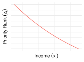
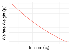
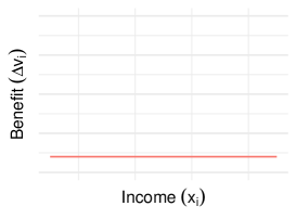
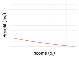
To demonstrate the intuition behind our method, we illustrate with a simple example in Figure 1. Consider the case of a single outcome and one dimension of heterogeneity, , which corresponds to income. A policymaker allocates a program by ordering households by the function , prioritizing poor households. As shown in Figure 1, depending on how treatment effects vary with , the same allocation could result from (1) higher welfare weights on the poor, (2) equal welfare weights, or (3) higher welfare weights on the rich. Likewise, in the case where is binary, an allocation to one group can result from (i) higher welfare weights, if that group benefits the same or less; (ii) equal welfare weights, if that group benefits more; or (iii) lower welfare weights, if that group benefits much more.
The next section demonstrates how to empirically recover welfare and impact weights from data in when there are multiple dimensions of heterogeneity and multiple outcomes of interest.
| An allocation rule that prioritizes the poor (low ) | |
 |
|
| Could result from | |
| (1) Higher welfare weight on the poor | if treatment effects are constant |
 |
 |
| (2) Equal welfare weights on households | if treatment effects are higher for the poor |
 |
 |
| (3) Higher welfare weight on the rich | if treatment effects are much higher for the poor |
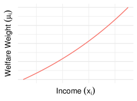 |
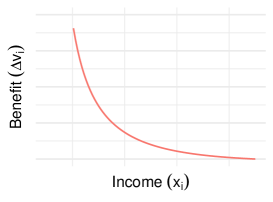 |
3 Estimation
Estimation proceeds in two steps:
We first predict the effect of treatment on each outcome , which may be heterogeneous as a function of covariates . This can be done using a variety of methods for estimating heterogeneous treatment effects, such as Wager and Athey’s (2018) machine learning approach, which works well when there is experimental variation in treatment assignment.666For treatment effect heterogeneity, covariates need only be correlated with impacts, so one may wish to include a large set of covariates in . In contrast, the choice of determines which characteristics to allow favoritism over, so one may wish to justify a smaller set.
Then, given that the policy achieves effects estimated to be , we ask what preferences (i.e., , the vector , and ) would be consistent an allocation according to the given ranking ()? If household is prioritized over (), equation (1) implies:
This problem can be modeled with an ordinal logit likelihood if we make the common assumption that the ranking error is distributed extreme value type-I: . Then, the logit likelihood of this particular placement of in the ranking is:
| (2) |
where represents the set of households ranked lower than household .
The logit likelihood of the full observed ranking is therefore
We use maximum likelihood to estimate the functions and and parameters and that best match the observed data . Unlike standard discrete choice settings where partial orderings are observed for multiple decisionmakers, we observe a single ordering of all alternatives. For this type of ranked data, we follow the exploded logit likelihood described by Train (2009).
Standard errors are computed by bootstrapping the entire procedure (accounting for uncertainty in both treatment effects and preference parameters). Individuals are drawn with replacement, and these bootstrapped samples are used to compute treatment effects, and then welfare and impact weights.
In many settings, we may not observe a full ranking or score, but rather a binary allocation of beneficiaries and non-beneficiaries (). This corresponds to a ranking with two levels. In such settings, the same procedure described above can be applied.
3.1 Parameterization
Our framework will work with general functional forms for and . In the empirical application that follows in Section 4, we model welfare weights as multiplicative:
We model the relative weight on outcome as the same for all households, , because our sample is not large enough to differentiate heterogeneity on these dimensions.
3.2 Identification
Preferences are identified based on how the policy’s ranking () varies with characteristics () and with treatment effects on components of utility ().
Unobservables
Our approach estimates the preferences that are consistent with the implemented policy , given the estimates of impact . This can be thought of as an ex-post audit. Our estimates will recover an observed component of welfare, , that is uncorrelated with any unobserved component, . There are several reasons why these implied preferences might differ from the actual preferences of the policymaker.
First, implied preferences could differ from policymaker preferences if the policymaker based the ranking on correlated unobservables. For example, if a policymaker is racially biased but an analyst does not allow race to enter modelled preferences, the policy may be found to be consistent with a preference for an income level that is correlated with race. In such settings, the method still reveals preferences that are consistent with the policy’s values, under the given specification of preferences.777This is analogous to the way that ordinary least squares recovers the best linear predictor given included variables, even in the presence of omitted variables. The specification of preferences (i.e., which variables they are defined over and their functional form) is thus a substantive decision. For this reason, practical applications should include both characteristics that policymakers wish to prioritize as well as characteristics for which there may be concerns of bias.
Second, implied preferences could differ from policymaker preferences if the policymaker has incorrect beliefs about these impacts at the time of the decision. If that were the case, upon observing the results of our method, the policymaker could change the policy to better align with their preferences. The method thus provides a tool for course correction.
The method can also be applied in cases where there is no single policymaker—for example, where allocations are the result of deliberations between constituents. In that case, our method will reveal social preferences consistent with the final allocation.
Sufficient variation
Identification also requires sufficient variation. It requires that some households benefit more than others. Welfare weights are primarily identified based on heterogeneity in impacts on the numeraire utility . If treatment effects were homogenous, it would not possible to separately identify and (their combination may be identified, in which case our method would collapse down to a standard exploded logit that does not account for treatment effects).
Identification of also requires that treatment has different impacts on different components of utility. Impact weight is identified from the relative ranking of households that are impacted more or less on utility component than on the numeraire (). If the treatment effects were heterogeneous but colinear between different components of utility, it would be possible to identify but not , because the data would not reveal how different components of utility influence the ranking.
The resulting parameters reveal which characteristics are correlated with being prioritized. If includes both a relevant variable as well as an irrelevant but colinear variable , the method will have imprecise estimates of the contribution of both, in a similar manner as a standard regression would. In that sense, one may want to restrict analysis to characteristics that one believes may be relevant for differential preference. In our application, we use survey data to narrow down factors that should enter the targeting rule.
4 Application
To illustrate how our method can be used in applied settings, we use the case of PROGRESA, a large conditional cash transfer program in Mexico.
4.1 Background on PROGRESA
First implemented by the Mexican federal government in 1997, PROGRESA provided cash transfers to poor households. Transfers, which averaged 197 pesos per month (approximately $20 USD at the time), were conditioned on regular doctor’s visits and/or regular school attendance (John Hoddinott, 2004). Roughly 99% of enrolled households met these conditions (Simone Boyce, 2003).888For simplicity, our analysis does not account for the conditionality of the transfer. For a more detailed discussion of PROGRESA and its background, see Emmanuel Skoufias (2008), and Simone Boyce (2003).
Within poor communities, PROGRESA ranked households based on a ‘household poverty score’ that incorporated a variety of different characteristics (such as household structure, indigenous languages, occupation, income, housing materials, etc.).999The program defined poor communities as those with a high ‘village marginality index’, computed based on the proportion of households living in poverty, population density, and health and education infrastructure. We focus on the preferences implied by household poverty scores, which were the basis for determining which households within a community eligible for the program. The score was computed in three steps. First, each household was classified as poor or not poor based on per capita income. Second, that poverty classification was approximated using discriminant analysis based on household characteristics (Skoufias et al., 1999). Third, the list of eligible households was presented in meetings in each community for review; a small number of households changed classification as a result. Our focus is on understanding which underlying values are consistent with the allocation resulting from this method of determining eligibility for the program.
During its initial implementation, PROGRESA administrators used a staggered roll-out to randomize when villages could enroll in the program: of the 506 villages included in the evaluation, 320 were randomly assigned to treatment, and initiated into the program in summer 1998. 186 communities were assigned to control and were not initiated into the program until 2000. Behrman and Todd (1999) show that the randomization across communities was successful in that treatment and control communities were statistically indistinguishable across a wide array of observable covariates.
Data
Our analysis relies on two distinct sources of data. The first is a standard household survey conducted in October 1998 (baseline) and November 1999 (endline). These capture household demographics, socioeconomic characteristics, health care utilization, and educational attendance for 14,333 households over the entire experiment period – see Appendix Table A1 for summary statistics. We focus on the sample of 6,642 households over which our outcomes are defined, who have at least one child aged 5 or below and at least one child aged 6-16. Thus, our estimates will reveal the values implied by the rankings within households with children, and not between households with and without children in the relevant ages.
The second data source is a survey that we conducted in 2021 to understand the preferences of Mexican residents over how households should be prioritized for social assistance. We surveyed a sample of 315 Mexican residents to elicit preferences for which types of households should receive transfers, and what types of program impacts were most desirable, in a manner similar to Saez and Stantcheva (2016). The survey asked respondents which household attributes should be considered in the design of such a program, and relied on multiple price lists to elicit indifference points. For a complete description of this survey, see Appendix A3.
We focus on three welfare outcomes that were monitored in the household surveys: (i) logarithm of per-capita consumption; (ii) child health, measured as the average number of sick days per child aged 0-5; and (iii) school attendance, calculated as the average number of school days missed per child aged 6-16. We treat log consumption as our numeraire (), and allow the other two outcomes to enter the welfare function linearly ( for ).101010Gandelman and Hernandez-Murillo (2015) fails to reject a level of risk aversion consistent with logarithmic utility in Mexico, based on self-reported wellbeing. Previous studies have estimated significant treatment effects on all three outcomes using the same survey data (John Hoddinott, 2004; Emmanuel Skoufias, 2008; Simone Boyce, 2003; Djebbari and Smith, 2008). Note that the program could also have impacted other outcomes not measured; our method will assume that such impacts are either zero or not valued. In Section 4.3.2, we discuss implications and extensions of this simplifying assumption.
We define welfare weights over the top five characteristics that Mexican residents in our survey reported should be considered when targeting cash transfers (): income; number of people; and age, education, and indigenous status of the household head.
4.2 Characterizing the Decision Rule
As a first step, we characterize the decision rule, by indicating which types of households are observed to be ranked higher than others. Table 1 column 1 reports these results, where the contribution of household characteristics to the final ranking is estimated with a logit ranking model (i.e., our model’s likelihood equation (2) with constraints and , estimating the constrained weights ). We report coefficients transformed by log base 1.01 (), which can be interpreted as the number of successive 1% increments implied. This suggests that households that are indigenous are ranked 47% higher (). It also suggests that each 10% increase in income corresponds with a 2% decrease in ranking. Each additional household member is associated with a 14% () increase in ranking. However, the conventional regression in column 1 does not describe why these households are ranked highly; it could be that they benefit more (higher treatment effects) or that they are favored (higher welfare weights), as suggested in Figure 1.
| Household Poverty Score 1999 | ||
| Decision Rule | Implied Preferences | |
| (Prioritization) | Welfare Weights | |
| (number of 1% increments) | ||
| Indigenous | 38.57 (5.0) | -12.4 (4.2) |
| log(Income) | -24.9 (1.9) | -14.3 (5.4) |
| Household Size | 13.0 (0.8) | 5.6 (2.1) |
| Head Age | -2.31 (0.2) | -1.0 (0.6) |
| Education (HS or above) | -240.2 (848.5) | -39.9 (21.5) |
| Impact Weights | ||
| (log points of daily consumption) | ||
| Missed Schooling (per day) | -0.03 (0.17) | |
| Sickness (per child sick day) | 0.08 (0.05) | |
| Value Regardless of Impact | 0.47 (3.75) | |
| 0.17 (0.17) | ||
| 6642 | 6642 | |
-
•
Notes: Left column is computed using our method, without treatment effects included in the estimation. Right column is calculated using causal forests to estimate heterogeneous treatment effects (see Figure 2). In all columns, standard errors are computed using a two-step bootstrap procedure that accounts for uncertainty in both treatment effects and preference parameters. Observations are drawn with replacement before estimation of the treatment effects and the welfare and impact weights. Treatment effects are then estimated from these bootstrapped samples, and welfare and impact weights estimated from these bootstrapped treatment effect estimates; the standard errors reported are the standard deviation across bootstrapped welfare and impact weight estimates.
4.3 Results: Estimating What Policies Value
Our main results from the PROGRESA example show how our method can decompose an observed allocation into the values implied by the decision rule.
4.3.1 Heterogeneity in Treatment Effects
As has been documented in prior work, the PROGRESA program significantly increased household welfare. On average over our sample, PROGRESA increased log household monthly consumption by 0.135, reduced the number of sick days per child by 0.18, and reduced the number of school days missed per child by 0.005.
However, these treatment effects were heterogeneous. We estimate this heterogeneity using Wager and Athey’s (2018) causal forest method, which recovers heterogeneous treatment effects nonparametrically, and includes restrictions to limit overfitting. Figure 2 shows that different households benefit by different amounts across the three outcomes. In particular, the program increased the consumption of indigenous households more than non-indigenous households. This can be seen in the fact that indigenous status is the most important feature in the causal forest (Appendix Table A2, column 1). The heterogeneity by indigenous status is also evident in Appendix Figure A1, which shows residualized treatment effects, estimated after removing variation explained by the other covariates.
While our main analysis relies on causal forests, which allow for more flexible and precise estimates of heterogeneity than linear models, the approach described in Section 3 can be used with alternative methods for estimating heterogeneous treatment effects. Corresponding results for OLS are reported in Appendix Section A4 and Appendix Figure A2.111111Comparing the causal forest estimates in Appendix Figure A1 with the OLS estimates in Appendix Figure A2, the relative flexibility of causal forests is apparent. While the general pattern of heterogeneity is often consistent across both methods, the causal forest method better captures non-linearity.
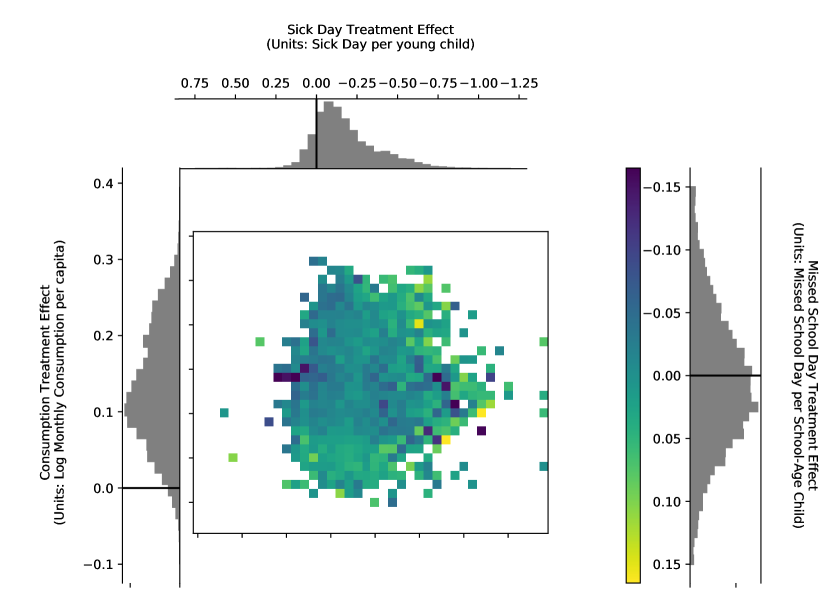
Notes: Heterogeneous treatment effects of PROGRESA, estimated using causal forests Wager and Athey (2018). Histograms show marginal treatment effects on log Consumption (left), Health (top), and School Attendance (right). Center figure shows joint distribution, where each cell corresponds to a combination of consumption and health treatment effects, and is colored according to average treatment effect on attendance. Households without at least one young and one school-age child are omitted from the figure.
4.3.2 Implied Policy Preferences
Next, given that we predict the policy would have impacts on household , we use our method to back out the implied preferences consistent with ranking that household at position . Table 1 column 2 reports the preferences that are consistent with the ranking . The first block of rows shows the implied welfare weights (), and the second block shows implied impact weights ( and ) and the standard deviation of the error term ().
We find that when the differential benefit that indigenous households face is accounted for, the decision rule actually implicitly places lower welfare weight on indigenous households (by ). Likewise, part of the negative weight on higher-income households can be explained by slightly lower marginal treatment effects for consumption for those households, and so the model infers moderately less negative implicit welfare weight on income when taking these heterogeneous treatment effects into account.
Our estimates of weights on different impacts are imprecise, so we focus on the bounds implied by 95% confidence intervals. These suggest that the Mexican government’s initial allocation rule is consistent with valuing each day of school attendance at less than 36% of daily per capita consumption (the point estimate suggests a positive value of 3%). They also suggest that the rule is consistent with valuing each prevented sick day per young child at less than 2% of daily per capita consumption (the point estimate actually suggests a negative value of 8%). The bounds for the value of schooling cover estimates of the returns to schooling from the literature; based on a review of multiple studies, Psacharopoulos and Patrinos (2018) suggest a 9% average return to a year of schooling.
Most of the implied value of the program comes from its impact on consumption, followed by the effect of providing the program independent from its effect on measured outcomes (the constant term ). The value of of 0.47 log points corresponds with an average of 179.4 pesos of consumption per person per month. The fact that this is larger than the average transfer of 33.9 pesos per person per month (John Hoddinott, 2004) suggests that the policy may implicitly value a peso of recipient consumption less than a peso of transfer. (Our estimates denominated in pesos are relative to the value placed on consumption gains.)
| (1) | (2) | (3) | |||
| Implied Preferences (Estimated) | Stated Preferences | ||||
| (1999 Pov. Score) | (2003 Pov. Score) | (Resident survey) | |||
| Welfare Weights (number of 1% increments) | |||||
| Indigenous | -12.4 (4.2) | 1.5 (3.0) | -6.1 (6.4) | ||
| log(Income) | -14.3 (5.4) | -1.8 (1.4) | -20.2 (8.5) | ||
| Household Size | 5.6 (2.1) | 1.9 (1.3) | 1.6 (2.0) | ||
| Head Age | -1.0 (0.6) | -0.03 (0.07) | 0.4 (0.3) | ||
| Education (HS or higher) | -39.9 (21.5) | -9.8 (7.8) | -6.3 (3.6) | ||
| Impact Weights (log points of daily consumption) | |||||
| Missed Schooling (per day) | -0.03 (0.17) | 0.02 (0.2) | -0.35 (0.15) | ||
| Sickness (per child sick day) | 0.08 (0.05) | 0.16 (0.12) | -0.34 (0.15) | ||
| Value Regardless of Impact | 0.47 (3.75) | 2.82 (12.52) | . | ||
| 0.17 (0.17) | 0.31 (0.28) | . | |||
| N | 6642 | 6642 | 310 | ||
-
•
Notes: Columns 1-2 are estimated using our method, using causal forests to estimate heterogeneous treatment effects. Column 1 estimates model using 1999 poverty scores; column 2 using 2003 poverty scores. Column 3 indicates stated preferences based on a survey of Mexican residents. Standard errors in columns 1-2 are computed using a two-step bootstrap procedure that accounts for uncertainty in both treatment effects and preference parameters. We exclude bootstrap draws (0 draws for the 1999 ranking, 1 draw for the 2003 ranking, out of 50 for each) that converged to corner solutions against the zero lower bound for omega. Standard errors in column 3 are computed directly from survey responses.
4.3.3 Alternative Preferences
Our framework also makes it possible to compare the preferences consistent with alternative policies. For instance, in the PROGRESA case, the Mexican government expanded the program in 2003, using a different poverty score to increase the priority of older and smaller households (Skoufias et al., 2001b). As shown in column 2 of Table 2, our method reveals that this new poverty score implicitly placed more welfare weight on richer households, and slightly less weight on larger and younger households. The impact weights are also imprecisely estimated; the 95% confidence intervals suggest the valuation of a missed day of school below 36% of consumption and of a young child sick day below 7% of consumption.
Table 2 also illustrates how the implemented policy (column 1) compares to the median stated preferences of residents, as reported in the survey we conducted in 2021 (column 3). The welfare weights implied by the implemented policy are similar to resident preferences: we fail to reject differences in all but age of the household head (which is small in magnitude). On average, survey respondents value impacts on children more: sick days at 34% of daily consumption and school attendance at 35% of daily consumption, though both of these estimates are imprecise.
4.4 Counterfactuals
We next consider the reverse problem: given preferences, what would the resulting policy look like? In the PROGRESA example, Table 3 compares the policy’s true allocation (column 1) to counterfactual allocations that would have resulted from alternative preferences (columns 2-6). Panel A indicates which preferences are used. We allow the welfare weights to be those estimated from the 1998 policy (columns 1, 4-6), those elicited from the resident survey (column 2), or fixed to weight all households equally (column 3). We allow the impact weights to be those estimated from the 1998 policy (columns 1 and 3), those elicited from the resident survey (column 2), or to only value one outcome (columns 4-6). Panel B indicates the decision rule implied by those preferences. Panel C shows the average outcomes that would be expected under the hypothetical policy, assuming it treated the same number of households as the implemented policy.
| (1) | (2) | (3) | (4) | (5) | (6) | ||
| HH Poverty | Resident | Equal Welfare | Policy only values impact on: | ||||
| Score | Preferences | Weights | Education | Health | Consumption | ||
| Panel A: Preferences | |||||||
| Welfare Weights | Estimated | From survey | Unity | Estimated | Estimated | Estimated | |
| Impact Weights | Estimated | From survey | Estimated | Only education | Only health | Only consumption | |
| Panel B: Implied decision rule (priority over covariates, in 1% increments) | |||||||
| Indigenous | 38.6 | 17.2 | 143.3 | -48.2 | 53.0 | 176.2 | |
| log(Income) | -24.9 | -88.4 | -10.0 | 89.8 | -28.5 | -26.4 | |
| Household Size | 13.0 | 15.0 | 2.31 | -13.8 | 4.3 | 8.9 | |
| Head Age | -2.3 | 3.3 | -0.6 | -10.8 | -1.1 | -1.6 | |
| Education | -240.2 | 32.4 | 12.7 | 24.2 | -93.9 | -49.8 | |
| Panel C: Counterfactual outcomes (monthly) | |||||||
| Log Consumption (pesos) | 4.852 | 4.853 | 4.875 | 4.849 | 4.843 | 4.874 | |
| Missed school (days/child) | 0.168 | 0.167 | 0.164 | 0.140 | 0.171 | 0.165 | |
| Sickness (sick days/child) | 0.637 | 0.609 | 0.655 | 0.647 | 0.567 | 0.635 | |
| 6642 | 6642 | 6642 | 6642 | 6642 | 6642 | ||
-
•
Notes: Table shows the distributional and outcome effects of designing decision rules using our framework. Panel A indicates which weights are used to prioritize households. Column 1 uses the ranking assigned by PROGRESA. Column 2 uses preferences elicited in a survey we conducted of Mexican residents. Column 3 projects the ranking as though the policy did not prioritize certain types of households, and was based on preferences over outcomes estimated in Table 2. Columns 4-6 indicate what would have happened if the policy used the estimated weights over households but only valued about impacts on education/health/consumption. Panel B shows the distributional effects of each column’s preferences, by estimating the implied priority ranking across households. Panel C shows each policy’s expected average outcomes, calculated using estimates of heterogeneous treatment effects.
Survey-based estimates of resident preferences
Column 2 shows the allocation that would result from imposing the preferences of residents as revealed by the survey. Relative to the actual policy in column 1, the hypothetical policy in column 2 reduces the prioritization of indigenous households, and increases the prioritization of poor households. Other household attributes are similarly prioritized under the two policies. In Panel C, we see that the policy consistent with resident preferences would slightly reduce child sickness relative to the implemented policy.
Alternate welfare weights
When welfare weights are set equal across households (column 3), the resulting score prioritizes indigenous households by a much larger factor, and lowers the priority given to lower income and larger households.
Prioritizing specific welfare outcomes
While in practice implemented policies may balance multiple outcomes, in columns 4-6 of Table 3, we present counterfactual allocations that would result in the extreme case where a policy was designed to improve only a single outcome. For instance, a policy designed to maximize education would prioritize smaller households and those with higher income (column 4). On the other hand, if only health effects were valued, the policy would slightly increase the prioritization of indigenous households (column 5). Finally, a policy that maximized consumption with no explicit consideration of health or education (column 6) would place much greater priority on households where the head is indigenous and reduce the penalty on education.
Understanding the policies that would result from extreme preferences can help in understanding the full set of potential policies, and what those policies imply. In the PROGRESA case, Figure 3 characterizes the frontier of possible average welfare impacts that would result from different allocations of the program. This frontier is shown as a convex hull with contour lines; the labeled points correspond to the policies given in the columns of Table 3. Policies that only value a single outcome lie at the corners of the outcome space. The implemented program (‘HH Poverty Score’) is close to the allocation consistent with the survey of Mexican residents preferences; neither are quite on the frontier with respect to unweighted outcomes, but both are close. (They are on the frontier of outcome spaces scaled by the corresponding welfare weights, see Appendix Figure A5.) More broadly, this method makes it possible to navigate program design in outcome space, rather than implementation space.
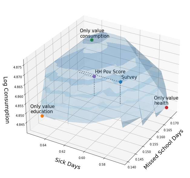
Notes: Figure shows the frontier of possible average welfare impacts that would have resulted from different allocations of PROGRESA. Each axis indicates the expected average impacts for a given welfare outcome. Labeled points correspond to particular allocations described in Table 3. Appendix Figure A5 shows the frontier when outcomes are scaled by welfare weights.
4.5 Extensions
If only an allocation is observed
In many settings, priority rankings are not available. Our method can still be used when the analyst observes only the final allocation (e.g., who receives the program, or who is admitted). This is because the binary indicator of whether a household received an allocation represents a (short) ranking. In the PROGRESA example, Table A3 demonstrates that when our method is applied to a binary allocation (), point estimates are similar to those reported in Table 1. Though the estimates are much less precise under the binary allocation, the qualitative insights are the same.
Testing models of welfare
The method can also be used to test whether policies are internally consistent with a postulated welfare function. If there is more than one potential treatment or policy, one could test the hypothesis that they apply the same welfare weights for each one. If that hypothesis is rejected, one can rule out that the policies are consistent with utilitarianism, given ex post information.
5 Conclusion
Policy discussions commonly revolve around the mechanics of implementation, rather than more fundamental notions of utility and welfare weights. This paper demonstrates how these discussions can be inverted. We provide a method to recover the primitives consistent with observed policies, using a model of preferences in conjunction with modern methods for estimating heterogeneous treatment effects, and demonstrate how to convert between welfare and allocation space.
We develop this approach and apply it to a large anti-poverty program in Mexico, to estimate the preferences consistent with the program’s implementation. This analysis reveals that, after accounting for heterogeneity in treatment effects, the program’s allocation placed higher weight on the welfare of poor and large families, and lower weight on indigenous households. The implied value of each missed school day and child sick day is estimated imprecisely but our confidence intervals do not rule out valuations estimated in prior work.
This framework could be used in several ways. To begin, it could be used to characterize the realized allocations of an existing program, to provide an indication of the preferences they imply. This, in turn, can provide a way to audit an existing program, to help hold policymakers accountable for past decisions – and in particular, to evaluate whether the implemented allocation reflects the stated goals of the policy. Perhaps most importantly, this approach can be used to adjust existing policies to better align with those goals.
References
- (1)
- Alatas et al. (2012) Alatas, Vivi, Abhijit Banerjee, Rema Hanna, Benjamin A. Olken, and Julia Tobias, “Targeting the Poor: Evidence from a Field Experiment in Indonesia,” American Economic Review, June 2012, 102 (4), 1206–1240.
- Alderman et al. (2019) Alderman, Harold, Jere R Behrman, and Afia Tasneem, “The Contribution of Increased Equity to the Estimated Social Benefits from a Transfer Program: An Illustration from PROGRESA/Oportunidades,” The World Bank Economic Review, October 2019, 33 (3), 535–550.
- Athey and Wager (2020) Athey, Susan and Stefan Wager, “Policy Learning with Observational Data,” arXiv:1702.02896 [cs, econ, math, stat], September 2020. arXiv: 1702.02896.
- Barocas et al. (2018) Barocas, Solon, Moritz Hardt, and Arvind Narayanan, Fairness and Machine Learning, fairmlbook.org, 2018.
- Barr (2012) Barr, Nicholas, Economics of the welfare state, Oxford university press, 2012.
- Behrman and Todd (1999) Behrman, Jere R. and Petra E. Todd, “Randomness in the experimental samples of PROGRESA (education, health, and nutrition program),” International Food Policy Research Institute, Washington, DC, 1999.
- Simone Boyce (2003) Boyce, Paul Gertler Simone, “An Experiment in Incentive-Based Welfare: The Impact of PROGRESA on Health in Mexico,” in “,” Vol. 85 Royal Economic Society 2003.
- Coady (2006) Coady, David P., “The Welfare Returns to Finer Targeting: The Case of The Progresa Program in Mexico,” International Tax and Public Finance, May 2006, 13 (2-3), 217–239.
- Coate and Morris (1995) Coate, Stephen and Stephen Morris, “On the Form of Transfers to Special Interests,” Journal of Political Economy, December 1995, 103 (6), 1210–1235.
- Djebbari and Smith (2008) Djebbari, Habiba and Jeffrey Smith, “Heterogeneous impacts in PROGRESA,” Journal of Econometrics, July 2008, 145 (1), 64–80.
- Dwork et al. (2012) Dwork, Cynthia, Moritz Hardt, Toniann Pitassi, Omer Reingold, and Richard Zemel, “Fairness through awareness,” in “Proceedings of the 3rd innovations in theoretical computer science conference” ACM 2012, pp. 214–226.
- Ensign et al. (2017) Ensign, Danielle, Sorelle A. Friedler, Scott Neville, Carlos Scheidegger, and Suresh Venkatasubramanian, “Runaway Feedback Loops in Predictive Policing,” arXiv:1706.09847 [cs, stat], June 2017. arXiv: 1706.09847.
- Filmer and Pritchett (2001) Filmer, Deon and Lant H. Pritchett, “Estimating Wealth Effects Without Expenditure Data—Or Tears: An Application To Educational Enrollments In States Of India*,” Demography, February 2001, 38 (1), 115–132.
- Fleurbaey and Maniquet (2018) Fleurbaey, Marc and Francois Maniquet, “Optimal income taxation theory and principles of fairness,” Journal of Economic Literature, 2018, 56 (3), 1029–79.
- Gandelman and Hernandez-Murillo (2015) Gandelman, Nestor and Ruben Hernandez-Murillo, “Risk Aversion at the Country Level,” SSRN Scholarly Paper ID 2646134, Social Science Research Network, Rochester, NY 2015.
- Gechter et al. (2019) Gechter, Michael, Cyrus Samii, Rajeev Dehejia, and Cristian Pop-Eleches, “Evaluating Ex Ante Counterfactual Predictions Using Ex Post Causal Inference,” arXiv:1806.07016 [stat], July 2019. arXiv: 1806.07016.
- Gertler (2004) Gertler, Paul, “Do Conditional Cash Transfers Improve Child Health? Evidence from PROGRESA’s Control Randomized Experiment,” The American Economic Review, 2004, 94 (2), 336–341.
- Greco et al. (2019) Greco, Salvatore, Alessio Ishizaka, Menelaos Tasiou, and Gianpiero Torrisi, “On the Methodological Framework of Composite Indices: A Review of the Issues of Weighting, Aggregation, and Robustness,” Social Indicators Research, January 2019, 141 (1), 61–94.
- Hanna and Olken (2018) Hanna, Rema and Benjamin A. Olken, “Universal Basic Incomes versus Targeted Transfers: Anti-Poverty Programs in Developing Countries,” Journal of Economic Perspectives, November 2018, 32 (4), 201–226.
- Haushofer et al. (2022) Haushofer, Johannes, Paul Niehaus, Carlos Paramo, Edward Miguel, and Michael Walker, “Targeting impact versus deprivation,” Working Paper, 2022.
- Hendren (2019) Hendren, Nathaniel, “Efficient Welfare Weights,” Working Paper 20351, National Bureau of Economic Research 2019.
- John Hoddinott (2004) Hoddinott, Emmanuel Skoufias John, “The Impact of PROGRESA on Food Consumption,” Economic Development and Cultural Change, 2004, 53 (1), 37–61.
- Hu and Chen (2018) Hu, Lily and Yiling Chen, “Welfare and Distributional Impacts of Fair Classification,” arXiv:1807.01134 [cs, stat], July 2018. arXiv: 1807.01134.
- Jayachandran et al. (2021) Jayachandran, Seema, Monica Biradavolu, and Jan Cooper, “Using Machine Learning and Qualitative Interviews to Design a Five-Question Women’s Agency Index,” Technical Report w28626, National Bureau of Economic Research March 2021.
- Kasy and Abebe (2020) Kasy, Maximilian and Rediet Abebe, “Fairness, equality, and power in algorithmic decision making,” in “ICML Workshop on Participatory Approaches to Machine Learning” 2020.
- Kitagawa and Tetenov (2018) Kitagawa, Toru and Aleksey Tetenov, “Who Should Be Treated? Empirical Welfare Maximization Methods for Treatment Choice,” Econometrica, 2018, 86 (2), 591–616. _eprint: https://onlinelibrary.wiley.com/doi/pdf/10.3982/ECTA13288.
- Liu et al. (2018) Liu, Lydia T., Sarah Dean, Esther Rolf, Max Simchowitz, and Moritz Hardt, “Delayed Impact of Fair Machine Learning,” in “Proceedings of the 35th International Conference on Machine Learning,” Vol. 80 of Proceedings of Machine Learning Research Stockholm, Sweden 2018, pp. 3156–3164.
- McKenzie (2005) McKenzie, David J., “Measuring inequality with asset indicators,” Journal of Population Economics, June 2005, 18 (2), 229–260.
- Mouzannar et al. (2018) Mouzannar, Hussein, Mesrob I. Ohannessian, and Nathan Srebro, “From Fair Decision Making to Social Equality,” arXiv:1812.02952 [cs, stat], December 2018. arXiv: 1812.02952.
- Nichols and Zeckhauser (1982) Nichols, Albert L. and Richard J. Zeckhauser, “Targeting Transfers through Restrictions on Recipients,” The American Economic Review, 1982, 72 (2), 372–377.
- Noriega et al. (2018) Noriega, Alejandro, Bernardo Garcia-Bulle, Luis Tejerina, and Alex Pentland, “Algorithmic Fairness and Efficiency in Targeting Social Welfare Programs at Scale,” Bloomberg Data for Good Exchange Conference, 2018.
- Psacharopoulos and Patrinos (2018) Psacharopoulos, George and Harry Anthony Patrinos, “Returns to investment in education,” 2018.
- Ravallion (2009) Ravallion, Martin, “How Relevant Is Targeting to the Success of an Antipoverty Program?,” The World Bank Research Observer, 2009, 24 (2), 205–231.
- Rolf et al. (2020) Rolf, Esther, Max Simchowitz, Sarah Dean, Lydia T. Liu, Daniel Björkegren, Moritz Hardt, and Joshua Blumenstock, “Balancing Competing Objectives with Noisy Data: Score-Based Classifiers for Welfare-Aware Machine Learning,” in “” 2020.
- Saez and Stantcheva (2016) Saez, Emmanuel and Stefanie Stantcheva, “Generalized Social Marginal Welfare Weights for Optimal Tax Theory,” American Economic Review, January 2016, 106 (1), 24–45.
- Skoufias et al. (1999) Skoufias, Emmanuel, Benjamin Davis, and Jere R. Behrman, “An evaluation of the selection of beneficiary households in the education, health, and nutrition program (PROGRESA) of Mexico,” International Food Policy Research Institute, Washington, DC, 1999.
- Skoufias et al. (2001a) , , and Sergio de la Vega, “Targeting the Poor in Mexico: An Evaluation of the Selection of Households into PROGRESA,” World Development, October 2001, 29 (10), 1769–1784.
- Skoufias et al. (2001b) , Sergio de la Vega, and Benjamin Davis, “Targeting the poor in Mexico,” FCND dicussion papers 103, 2001.
- Emmanuel Skoufias (2008) Skoufias, Vincenzo Di Maro Emmanuel, “Conditional Cash Transfers, Adult Work Incentives, and Poverty,” Journal of Development Studies, 2008, 44 (7), 935–960.
- Train (2009) Train, Kenneth E., Discrete Choice Methods with Simulation, 2 ed., Cambridge: Cambridge University Press, 2009.
- UNDP (1990) UNDP, “Human Development Report 1990: Concept and Measurement of Human Development,” Technical Report 1990.
- Wager and Athey (2018) Wager, Stefan and Susan Athey, “Estimation and Inference of Heterogeneous Treatment Effects using Random Forests,” Journal of the American Statistical Association, July 2018, 113 (523), 1228–1242.
- Wang (2020) Wang, Fan, “The Optimal Allocation of Resources Among Heterogeneous Individuals,” Available at SSRN, 2020.
Appendices
A1 Generalized curvature in utility components
This section considers what will be measured if the utility functions are assumed to be linear () but in fact the true utility functions have curvature. The true impact of the program on component of utility is then:
Taking a Taylor approximation from the factual level , we have . Thus for any we have:
We can then express the utility benefit of treating as:
This implies that if we do not specifically account for curvature and estimate a linear model, the welfare and impact weights we estimate ( and ) are approximately a combination of the underlying welfare and impact weights ( and ) and any curvature in the utility functions (), as long as the baseline value of the outcome () is included as a characteristic along which these weights can vary (). If the true utility is linear, then coincides with and with . Otherwise, utility curvature multiplies the weights.
A2 Data Cleaning Process
The data for the evaluation of PROGRESA is composed of household survey responses from a sample of 506 villages from seven states across multiple years. Three different survey years are used: a baseline survey in October 1997, and two follow-up surveys in October 1998 and November 1999. Villages were randomly assigned to a treatment group which received the program at the beginning, and a control groups, which received it two years later. Within villages in the treatment group, a poverty index score is computed based on household income and assets, and all households meeting the score requirement are eligible to receive the program’s conditional transfers.
We compute a measure of average household monthly consumption per member based on the survey responses. The October 1998 and November 1999 surveys ask households about the quantity consumed, quantity purchased and amount of money expended on 36 common food items, as well as expenditure for several non-food categories (in weekly/monthly/semi-annual amounts). We use the information regarding quantity purchased and amount of money expended to construct household-specific prices which are then multiplied by quantity consumed (this helps to account for the fact that households consume food that is self-produced in addition to bought). If household-specific information is missing, we use locality, municipality or state average prices (the smallest level available).
A3 Preference survey
We additionally survey Mexican residents to elicit their preferences for different allocations of social welfare programs. We solicited responses to a survey from a nationally representative sample of computer users in Mexico, through a Qualtrics survey panel.
A3.1 Survey design
After obtaining consent and an initial information screen, participants were asked their preferences for allocating benefits to different types of households. The survey was translated in Mexican Spanish. First, respondents were asked to select which attributes the government should consider when prioritizing which households receive cash transfers, from a list (age, income, household size, education, agricultural, indigenous, and gender). Second, subjects were asked to make monetary allocation decisions between different households using multiple price lists (see Figure A3 for an example). In each, one focal attribute differed between the households, and two other control attributes were held fixed. We randomized which controls were included, the order they were presented, and the scale of the tradeoff.121212Each participant saw base tradeoff numbers multiplied by 1x, 2x, or 3x, selected at random. Each subject filled in one price list for each focal attribute. Third, for a particular household, subjects were asked to make allocation decisions between money and education and child health using multiple price lists (see Figure A4). The description of the household included three randomly selected control attributes. Finally, subjects were asked for basic demographics.
A3.2 Estimation
We use the survey responses to estimate and :
To identify , compare impacts in dollars of consumption (where other impacts ). If individual differs from only in attribute and the crossover point is and , then
To identify , now instead hold fixed individual attributes, and consider impacts on different outcomes. If the crossover point is and then .
A3.3 Validation
The design included several checks to ensure that respondents took the survey seriously. First, prior to the survey, participants were asked, ‘We care about the quality of our survey data and hope to receive the most accurate measure of your opinions, so it is important to us that you thoughtfully provide your best answer to each question in the survey. Do you commit to providing your thoughtful and honest answers to the questions in this survey?’ Only participants who answered ‘I will provide my best answers’ were invited to continue with the survey. Second, after reading the instructions, participants responded to five simple questions to validate understanding of the study. In order to complete the study, participants had to respond correctly. Third, the survey included controls to ensure that participants spent adequate time on each question. The submit button for the main exercises appeared only after a 5 second delay.131313The implementation of this in Qualtrics made it possible for participants to advance if this time had elapsed, even if a multiple price list question had not been answered. For this reason, a handful of participants did not respond to all questions. Additionally, participants who were completing the survey too quickly (less than half the median elapsed time in the pilot survey) were removed from our sample, following a standard quality protocol used by Qualtrics. Fourth, in the final demographic survey, respondents were asked to rate the following three statements along the same Likert scale ranging from ‘Strongly Disagree’ to ‘Strongly Agree’: ‘I made each decision in this study carefully’, ‘I made decisions in this study randomly’, and ‘I understood what my decisions meant.’ A careful respondent should agree with the first and last statement but disagree with the middle; agreement or disagreement with all statements reveals that a respondent made careless decisions. We restrict the sample to only respondents who disagreed that they had made decisions randomly.141414Apart from two pilot respondents. 91% of respondents agreed with the first and last statement, and disagreed with the middle; 58% did so strongly.
There was an optional comment box at the conclusion of the survey; 49% of respondents filled in a comment, suggesting a high level of engagement with the survey. Although some respondents used the box to indicate some confusion with the selector interface, several respondent affirmatively to the approach of basing policy on resident preferences, such as (translated to English):
-
•
‘Excellent that they do these surveys to assess the policies of support to families’
-
•
‘I think this survey was very important since the benefits that sometimes come are the same for all people and the situations of each person are not considered. For some it may be enough but for others it is too little.’
-
•
‘excellent survey, hopefully and we could society decide these support, because that is how we would eradicate poverty’
A4 OLS Treatment Effect Estimates
A4.1 Estimation: OLS
One can also use linear regression to estimate heterogeneous treatment effects. We follow Djebbari and Smith (2008), allowing treatment effects to vary by age and gender composition of the household, total household size, and several characteristics of the household head: education level, indigenous status, gender, working in the agricultural sector, and age.151515We depart from Djebbari and Smith (2008) in that we omit poverty scores and village marginality index and their respective interactions in the list of covariates, to avoid potential correlated errors from using these rankings in both the treatment effect estimates and in the preference-learning method. Formally, we estimate:
| (3) |
where is the endline outcome, is the vector of baseline covariates, and is a dummy variable for treatment status of household . This model allows endline outcomes to differ systematically according to household covariates, and additionally allows the treatment effect of PROGRESA to differ across households according to their covariates.
We construct our variables for treatment effects from the predicted values from our estimated equation (3), as
A4.2 Results
On average over our sample, using OLS PROGRESA increased household log monthly consumption by 0.07, to have reduced the number of sick days per child by 0.22, and slightly increased the number of school days missed per child by 0.026 (very close to zero).
However, the effects of the program differ across households. The overall distributions of treatment effects by outcome for OLS, are presented in Figure A6. The distribution of estimated effects estimated under causal forest is tighter, in particular for the schooling and health outcomes. With OLS, we see a fairly strong correlation between health treatment effect estimates and schooling treatment effect estimates, but with causal forest this correlation is much less apparent.
OLS coefficient estimates are presented in Table A4, with standard errors in parentheses. Similar to Djebbari and Smith (2008), our OLS point estimates show that log consumption treatment impacts are higher for households with indigenous status.161616Note that our specification differs from Djebbari and Smith (2008) in that we exclude the ranking metrics from the list of covariates.
Appendix Exhibits
| October 1998 mean | |
| Head of household: | |
| … Is indigenous | 0.41 |
| … Age | 41.13 |
| … Education (HS or higher) | 0.005 |
| … Is male | 0.94 |
| … Is an agricultural worker | 0.65 |
| Household size | |
| … Number of children less than 6 years old | 1.97 |
| … Number of children 6-16 years old | 2.81 |
| … Number of adults 17+ years old | 2.54 |
| Log monthly average per capita consumption (log pesos) | 5.08 |
| Average number of days a school-age child misses school | 0.32 |
| Average number of days a young child is sick | 1.07 |
| Assigned to treatment group | 0.61 |
| N | 6537 |
-
•
Notes: Table shows the average levels in October 1998 of households matched to November 1999 survey sample. HS education defined as 12 years or more of education. Number of days a young child is sick, and number of days a school-age child misses school, are computed as an average over the number of children in the respective age group in the household. Sample restricted to only households with children in the targeted categories for health and schooling intervention (0-5 y.o., 6-16 y.o.) during the November 1999 survey.
| Log Consumption | Schooling | Health | |
| Monthly per capita | # days missed school | # Sick days | |
| (pesos) | per child | per child | |
| head age | 0.112 | 0.308 | 0.228 |
| household income 97 | 0.198 | 0.163 | 0.263 |
| head indigenous | 0.362 | 0.009 | 0.011 |
| num child 3 to 5 yrs | 0.01 | 0.072 | 0.162 |
| num child less than 2 yrs | 0.017 | 0.143 | 0.035 |
| num adults | 0.079 | 0.059 | 0.044 |
| num child 6 to 10 yrs | 0.074 | 0.02 | 0.044 |
| num men at least 55 yrs | 0.014 | 0.052 | 0.007 |
| head agricultural worker | 0.023 | 0.035 | 0.014 |
| num women 20 to 34 yrs | 0.009 | 0.026 | 0.037 |
| num boys 11 to 14 yrs | 0.011 | 0.03 | 0.023 |
| num men 20 to 34 yrs | 0.009 | 0.012 | 0.042 |
| num girls 11 to 14 yrs | 0.013 | 0.014 | 0.031 |
| num girls 15 to 19 yrs | 0.027 | 0.007 | 0.015 |
| num boys 15 to 19 yrs | 0.016 | 0.007 | 0.02 |
| male head of household | 0.005 | 0.023 | 0.004 |
| num women 35 to 54 yrs | 0.006 | 0.01 | 0.008 |
| num men 35 to 54 yrs | 0.008 | 0.006 | 0.007 |
| num women at least 55 yrs | 0.008 | 0.004 | 0.004 |
| head education | 0 | 0 | 0 |
| N | 6642 | 6642 | 6642 |
-
•
Notes: Feature importances as estimated from causal forest estimation of heterogeneous treatment impacts of PROGRESA on three outcome dimensions: log consumption (log monthly per capita consumption), schooling (number of missed school days per child), and health (number of sick days per child). Schooling and health sick days / missed school days measured over 28 days prior to survey. Estimates reflect 3 separate causal forest estimations for each respective outcome.
| Household Poverty Score | ||||
| Observe full | Observe only | |||
| ranking | binary allocation | |||
| Log Welfare Weights | ||||
| Indigenous | -12.4 (4.2) | -9.71 (61.1) | ||
| log(Income) | -14.3 (5.4) | -8.16 (32.7) | ||
| Household Size | 5.6 (2.1) | 3.3 (18.8) | ||
| Head Age | -1.0 (0.6) | -0.53 (17.0) | ||
| Education | -39.9 (21.5) | -19.2 (34.2) | ||
| Impact Weights | ||||
| Missed Schooling (per day) | -0.03 (0.17) | 0.02 (1.26) | ||
| Sickness (per child sick day) | 0.08 (0.05) | 0.11 (0.07) | ||
| Value Regardless of Impact | 0.47 (3.75) | 0.75 (109.21) | ||
| 0.17 (0.17) | 0.10 (0.1) | |||
| N | 6642 | 6642 | ||
-
•
Notes: Both columns computed using our method, using heterogeneous treatment effects estimated with causal forest (see Figure 2). Standard errors are computed using a two-step bootstrap procedure that accounts for uncertainty in both treatment effects and preference parameters. We exclude bootstrap draws (0 draws for full ranking, 1 draw for binary ranking, out of 50 for each) that converged to corner solutions against the zero lower bound for omega.
| Log Consumption | Schooling | Health | |
| (Monthly avg. per person, in pesos) | (Avg. days school missed per child) | (Avg. sick days per child) | |
| Treatment | -0.0271 (0.115) | -0.3527 (0.249) | -0.8111 (0.456) |
| Treatment X head indigenous | 0.1462 (0.027) | 0.0323 (0.058) | 0.0389 (0.106) |
| Treatment X log(Income 1997) | -0.0027 (0.02) | 0.0141 (0.042) | 0.06 (0.077) |
| Treatment X num adults | -0.0157 (0.012) | 0.0134 (0.027) | 0.0086 (0.05) |
| Treatment X head age | 0.0017 (0.002) | 0.0067 (0.004) | 0.0046 (0.007) |
| Treatment X head education | 0.0208 (0.003) | -0.0102 (0.007) | 0.0121 (0.014) |
| Treatment X male head of household | -0.0379 (0.063) | 0.1006 (0.137) | 0.1513 (0.251) |
| Treatment X head agricultural worker | 0.0523 (0.029) | -0.11 (0.062) | -0.0803 (0.114) |
| Treatment X num child less than 2 yrs | -0.0297 (0.016) | 0.0907 (0.034) | 0.0019 (0.063) |
| Treatment X num child 3 to 5 yrs | -0.0307 (0.019) | -0.0604 (0.041) | 0.1187 (0.075) |
| Treatment X num child 6 to 10 yrs | 0.0451 (0.015) | 0.015 (0.032) | -0.0178 (0.058) |
| Treatment X num boys 11 to 14 yrs | 0.0139 (0.021) | -0.0495 (0.045) | -0.0218 (0.082) |
| Treatment X num girls 11 to 14 yrs | 0.0212 (0.021) | -0.0279 (0.045) | 0.0315 (0.082) |
| Treatment X num boys 15 to 19 yrs | -0.024 (0.023) | 0.001 (0.051) | -0.0633 (0.093) |
| Treatment X num girls 15 to 19 yrs | -0.0243 (0.023) | 0.0035 (0.049) | 0.0558 (0.09) |
| Treatment X num men 20 to 34 yrs | 0.0037 (0.027) | -0.0224 (0.058) | -0.2424 (0.106) |
| Treatment X num women 20 to 34 yrs | 0.0044 (0.028) | 0.0439 (0.062) | 0.1897 (0.113) |
| Treatment X num men 35 to 54 yrs | 0.0479 (0.039) | -0.0492 (0.084) | 0.0115 (0.153) |
| Treatment X num women 35 to 54 yrs | -0.0225 (0.037) | 0.0198 (0.079) | -0.0142 (0.145) |
| Treatment X num men at least 55 yrs | -0.0416 (0.053) | -0.3011 (0.116) | -0.0174 (0.212) |
| Treatment X num women at least 55 yrs | -0.0283 (0.041) | 0.0372 (0.089) | -0.0739 (0.163) |
| Baseline Covariates | X | X | X |
| 0.180 | 0.0132 | 0.03 | |
| N | 6642 | 6642 | 6642 |
-
•
Notes: OLS coefficients of household characteristics interacted with treatment effects on three outcome dimensions: log consumption (log monthly per capita consumption), schooling (number of missed school days per child), and health (number of sick days per child). Schooling and health sick days / missed school days measured over 28 days prior to survey. Baseline covariates here includes the covariates without interaction with treatment effects, e.g. head age, as well as a constant term.
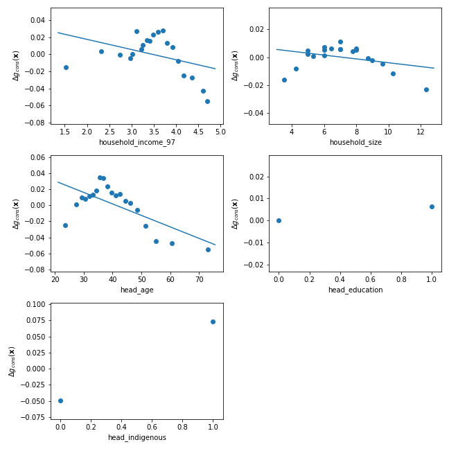
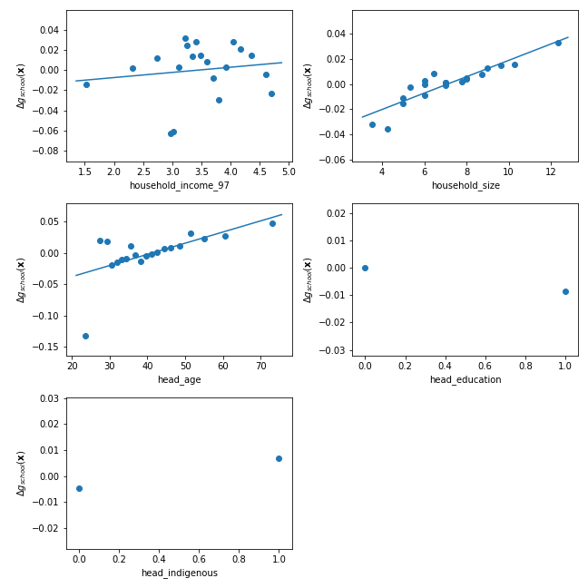
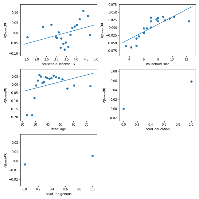
Notes: Binscatter plots of treatment effects from causal forest over a selected group of five covariates: household size; household head education; household head indigenous status; household head age; and log household income in the pre-period of 1997. Figures shown for treatment effects over per-person monthly consumption, number of sick days per child, and number of missed school days per child. Treatment effects shown are residualized against remaining covariates in the regression (the other graphed covariates).
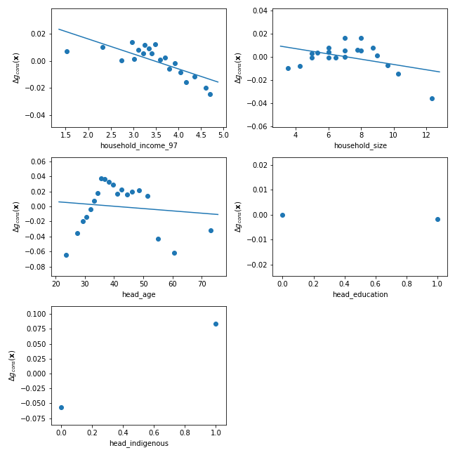
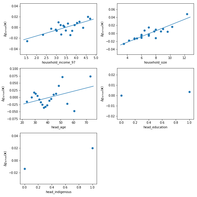
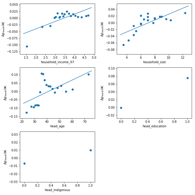
Notes: Binscatter plots of treatment effects from OLS over five covariates: household size; household head education; household head indigenous status; household head age; and log household income in the pre-period of 1997. Figures shown for treatment effects over per-person monthly consumption, number of sick days per child, and number of missed school days per child. Treatment effects shown are residualized against remaining covariates in the regression (the other graphed covariates).
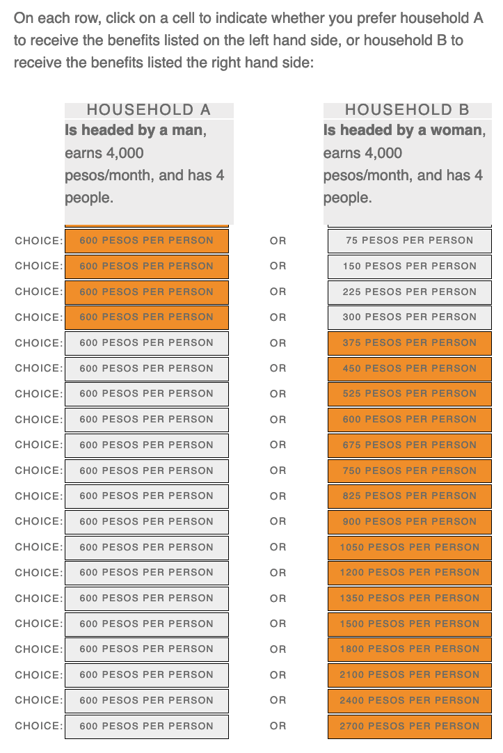
Notes: Respondents saw a version of this question translated into Spanish.
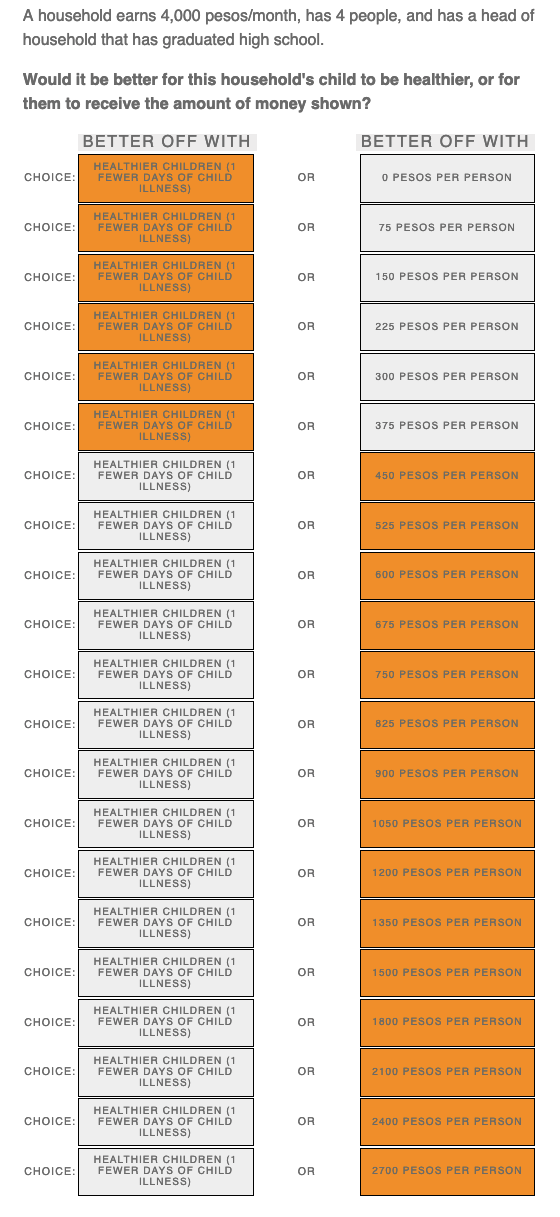
Notes: Respondents saw a version of this question translated into Spanish.
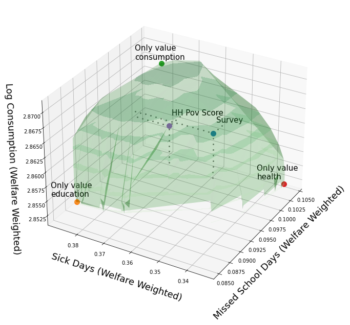
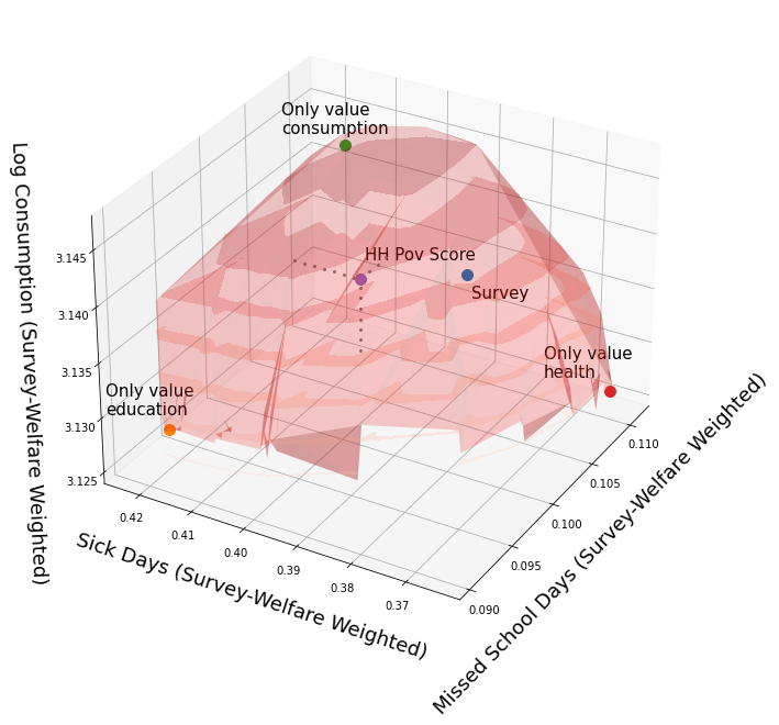
Notes: Figure shows the frontier of outcomes resulting from all possible allocations, weighted by welfare weights. Panel (a) weights outcomes by the welfare weights consistent with the implemented PROGRESA program, derived using our method. Panel (b) uses welfare weights consistent with the inferred preferences from the implemented survey. Labeled points correspond to particular allocations described in Table 3.
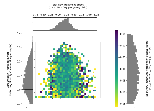
Notes: Joint and marginal distributions of estimated treatment effects of PROGRESA conditional cash transfer on schooling, health, and consumption, estimated using OLS. Schooling treatment effects are measured over the number of missed school days per school-age child in a given household. Health treatment effects are measured over the number of sick days per young (0-5 years old) child in a given household. Consumption treatment effects are measured over per-person consumption in pesos in a given household. Marginal distributions for consumption and health treatment effects are shown over the y and x axes, respectively, and are binned together in the center figure. Average schooling treatment effects in each consumption-health-treatment-effect bin is shown by the fill color of the bin, according to the index of the legend on the right. The marginal distribution of schooling treatment effects is shown in parallel to this legend. Note that missed school days and sick days are inferred to be ”bads”, according to our estimated weights, and so higher negative values for these treatment effects are associated with higher social utility. Note also that we drop households without children in the relevant age range for health and schooling treatment effects; the above graphs show only TEs for households for which these TEs are defined.