Superharmonic Instability of Stokes Waves

Abstract

A stability of nearly limiting Stokes waves to superharmonic perturbations is considered numerically. The new, previously inaccessible branches of superharmonic instability were investigated. Our numerical simulations suggest that eigenvalues of linearized dynamical equations, corresponding to the unstable modes, appear as a result of a collision of a pair of purely imaginary eigenvalues at the origin, and a subsequent appearance of a pair of purely real eigenvalues: a positive and a negative one that are symmetric with respect to zero. Complex conjugate pairs of purely imaginary eigenvalues correspond to stable modes, and as the steepness of the underlying Stokes wave grows, the pairs move toward the origin along the imaginary axis. Moreover, when studying the eigenvalues of linearized dynamical we find that as the steepness of the Stokes wave grows, the real eigenvalues follow a universal scaling law, that can be approximated by a power law. The asymptotic power law behaviour of this dependence for instability of Stokes waves close to the limiting one is proposed. Surface elevation profiles for several unstable eigenmodes are made available through http://stokeswave.org website.

I Introduction

A key object in ocean dynamics is a swell which is a spatially periodic train of surface gravity waves propagating in one direction with constant velocity. Such train is well described by Stokes waves discovered by Stokes Stokes (1847, 1880a, 1880b). These nonlinear long waves (with wavelengths typically in the range from meters to hundred of meters) propagate without change of form and are described by a potential flow of ideal (incompressible and inviscid) $2$-dimensional fluid with free surface and infinite depth. There is a long history of study of Stokes waves including Michell (1893); Nekrasov (1921); Grant (1973); Schwartz (1974); Longuet-Higgins and Fox (1977, 1978a); Toland (1978); Plotnikov (1982); Amick et al. (1982); Williams (1981, 1985); Tanveer (1991); Longuet-Higgins (2008); Dyachenko et al. (2013, 2016); Lushnikov (2016); Lushnikov et al. (2017).

A stability of Stokes waves determines an eventual fate of Stokes waves in ocean. We follow Longuet-Higgins (1978a) and Longuet-Higgins (1978b) to distinguish  superharmonic stability and subharmonic stability. Superharmonic stability means addressing perturbations with the same spatial period as the spatial period $\Lambda$ of Stokes wave (with the cases of the smaller spatial periods $\Lambda/n,n=2,3,\ldots$ of perturbations also included as particular cases). Subharmonic perturbations have larger period than $\Lambda.$ Subharmonic instability of deep water with small amplitudes has been extensively studied since Benjamin and Feir (1967); Lighthill (1965); Whitham (1967); Zakharov (1968). The same instability was discovered in Bespalov and Talanov (1966) for nonlinear optics. That instability is now called either by Benjamin-Feir instability or modulational instability, see also Zakharov and Ostrovsky (2009) for historical overview. Modulational instability is efficiently described by the approximation of nonlinear Schrödinger equation for the envelope of slowly modulated Stokes wave Zakharov (1968). A nonlinear stage of the development of that instability results in formation of solitons as well as in weak turbulence of surface gravity waves with dynamics of time scales greatly exceeding a period of Stokes wave. Another type is high frequency instability of Stokes waves of small amplitude which typically produces small growth rates, see Deconinck and Oliveras (2011); Creedon et al. (2022). Ref. Murashige and Choi (2020) provides a conformal mapping approach to linear stability of Stokes waves in irrotational and waves on shear current setting for both super- and subharmonic instability.

In this work, we focus on superharmonic instability of strongly nonlinear Stokes waves. Instability growth rate is much larger than the growth rate of modulational instability of small amplitudes waves. Thus this instability may play significant role in wavebreaking at the nonlinear stage of instability development. This is consistent with well-know oceanic observations, water tank experiments and large scale simulations that strongly nonlinear gravity waves quickly results in multiple wavebreaking events provided steepness $H/\Lambda$ exceeds $\approx 0.0178$  Banner and Tian (1998); Banner et al. (2000); Song and Banner (2002); Korotkevich et al. (2019).

A nonlinearity of Stokes wave is determined by a steepness $H/\Lambda$, where $H$ is the Stokes wave height defined as the vertical distance from the crest to the trough of Stokes wave. Without loss of generality we use scaled units at which a phase speed $c_{0}$ of linear gravity wave of wavelength $\Lambda$ is $c_{0}=1$ and we set $\Lambda=2\pi$ (see e.g. Dyachenko et al. (2016) for details of that scaling). In these units Stokes wave has a speed $c>1$ with the limit $H\to 0,\ c\to 1$ corresponding to the linear gravity wave. The Stokes wave of the greatest height $H=H_{max}$ (also called by the limiting Stokes wave) has the singularity in the form of the sharp angle of $2\pi/3$ radians on the crest Stokes (1880b). Refs. Dyachenko et al. (2016); Lushnikov et al. (2017) and a website http://stokeswave.org provide high precision numerical approximation for Stokes wave including the estimate $H_{max}/\Lambda=0.141063483980\pm 10^{-12}$.

In Longuet-Higgins (1978a) the superharmonic instability of Stokes waves was predicted at the steepness exceeding $H/\Lambda\approx 0.1388$ (Ref. Longuet-Higgins (1978a) used $ka$ for waves steepness with $k=2\pi/\Lambda$ and $a=H/2$ implying $ka=\pi H/\Lambda$) and suggested that the instability threshold corresponds to the maximum of $c$ as the function of $H/\Lambda$. In Tanaka (1983) the first computation of a growth rate of superharmonic instability was performed from the analysis of the eigenvalue problem of the linearization around Stokes wave and found that superharmonic instability has a threshold at $H/\Lambda=0.1366$, with one unstable mode appearing above that threshold. In addition, in Tanaka (1983) it was conjectured that this threshold corresponds to the first maximum of the total energy of Stokes wave as the function of $H/\Lambda$ in the contrast with the prediction of Longuet-Higgins (1978a). This conjecture was confirmed analytically in Saffman (1985) based on the Hamiltonian formulation of free surface dynamics Zakharov (1968), see also Bridges (2004) for more discussion. In Longuet-Higgins and Tanaka (1997a) it was found that as steepness of the Stokes wave increases past $H/\Lambda\approx 0.1366$ a second unstable mode appears at $H/\Lambda\approx 0.141$. It is natural to assume that as we approach the limiting Stokes waves, more unstable modes would appear. A nonlinear stage of the development of Stokes waves instability of all these modes typically results in wave breaking as were studied from simulations in multiple papers including Longuet-Higgins and Cokelet (1978); Longuet-Higgins and Dommermuth (1997a); Dyachenko and Newell (2016).

In this paper we provide numerical solution of eigenvalue problem for superharmonic instability and obtain three unstable branches. These branches originate from extrema of Stokes wave energy as a function of $H/\Lambda$. In particular, the first instability branch originates at $H_{1}/\Lambda=0.1366035\pm 10^{-7}$, the second branch at $H_{2}/\Lambda=0.1407965\pm 10^{-7}$ and the third branch at $H_{3}/\Lambda=0.1410496\pm 10^{-7}$. The accuracy of these numerical values can be further improved to any desired level by computing Stoke wave with variable precision following approaches of Dyachenko et al. (2013, 2016); Lushnikov (2016); Lushnikov et al. (2017). The latter paper discusses implementation of an auxiliary conformal mapping to improve the convergence rate of Fourier series representing Stokes solutions; this mapping was used to improve the numerical resolution of the eigenfunctions appearing in the linear stability analysis implemented in the present paper. We found that the dependence of these growth rates as functions of $H/\Lambda$ collapses into a universal curve via a shift and a rescaling of $H/\Lambda$ into $(H_{max}-H)/(H_{max}-H_{n})$, where $n=1,2,3$ is the number of the unstable eigenmode.

The paper is organized as follows. Section II.1 provides basic dynamic equations for free surface dynamics. Section II.2 considers a linearization of these equations and formulate an eigenvalue for the stability analysis of Stokes wave. Section II.3 describes a numerical approach to solve the large scale eigenvalue problem. A shift-invert method in combination with Arnoldi algorithm is used to address eigenvalues for large matrices up to $90,000\times 90,000$ of linearized problem. Section III provides the main results including the numerical results on three unstable branches in Section III.1 and a rescaling of these branches to the universal curve in Section III.2. Section IV summarizes the main results and discusses future directions.

II Formulation of the Problem

II.1 Dynamical equations of free surface dynamics

We consider a 2D flow of an ideal incompressible fluid with a free surface in a gravity field without surface tension. Fluid occupies the region $-\infty<x<\infty$ and $-\infty<y<\eta(x,t)$ with the elevation of the moving free surface given by the function $y=\eta(x,t)$ at a moment of time $t$. A gravity field is pointed in the negative direction of $y.$ We consider a potential flow with the velocity $\mathbf{v}$ represented through the scalar velocity potential $\Phi(x,y;t)$ as follows $\mathbf{v}=\mathbf{\nabla}\Phi$. The incompressibility condition $\mathrm{div}(\mathbf{v})=0$ requires the velocity potential to be a harmonic function $\nabla^{2}\Phi=0$. The kinematic boundary condition (BC)

$$\frac{\partial\eta}{\partial t}=\left.\left(-\frac{\partial\Phi}{\partial x}\frac{\partial\eta}{\partial x}+\frac{\partial\Phi}{\partial y}\right)\right|_{y=\eta(x,t)}$$ (1)

and dynamic BC

$$\quad\;\;\left.\left(\frac{\partial\Phi}{\partial t}+\frac{1}{2}\left(\mathbf{\nabla}\Phi\right)^{2}\right)\right|_{y=\eta(x,t)}+g\eta=0,$$ (2)

have to be satisfied on the free surface, where $g$ is the acceleration due to gravity. The kinematic BC means that the free surface moves together with fluid particles located at that surface, i.e. there is no separation of fluid particles from the free surface. The dynamic BC is given by the time-dependent Bernoulli equation at the free surface ensuring the zero pressure at the free surface. We also assume decaying boundary condition on the velocity potential deep inside fluid $\left.\Phi(x,y)\right|_{y\to-\infty}\to 0$. We consider periodic solutions thus focusing of one period of length $\Lambda$ with $x\in[-\Lambda/2,\Lambda/2]$ and periodic BC in $x$.

As a result, we have to solve Laplace equation $\nabla^{2}\Phi=0$ in time-dependent domain with the motion of of free surface determined by boundary conditions (1),(2) which form a closed set of equation. An efficient way to solve these equation is through the time-dependent conformal mapping $z(w,t)=x(u,v;t)+\mathrm{i}y(x,y;t)$ of a fixed domain (lower complex half-plane $\mathbb{C}^{-}$) of the auxiliary variable $w=u+\mathrm{i}v,$ $u,v\in\mathbb{R}$ into a time-dependent fluid domain in the physical complex plane $z=x+\mathrm{i}y$. Because of assumed $\Lambda$-periodicity in $x$, we restrict to one spatial period (along $u$) in $w$-plane as well, see Figure 1.

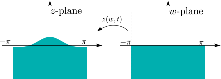
Figure 1: Half-strip in $w$ plane ($(u,v)\in[-\pi,\pi]\times(-\infty,0]$) into the area in $(x,y)$ plane under the free-surface $\eta(x,t)$. The line $v=0$ is mapped into the fluid surface.

The idea of using such type of time-dependent conformal transformation was exploited by several authors including Ovsyannikov (1973); Meison et al. (1981); Tanveer (1991, 1993); Dyachenko et al. (1996); Chalikov and Sheinin (1998, 2005). We follow Dyachenko et al. (1996) to recast equations (1) and (2) into the equivalent form for $x(u,0;t),\ y(u,0;t)$ and $\Psi(u,0;t)$ (here and below we abuse the notation and use the same symbol $\Psi$ for function of both $(x,y,t)$ and $(u,v,t)$) at the real line $w=u$ of the complex plane $w$ as follows

$$y_{t}=(y_{u}\hat{H}-x_{u})\left[\frac{\hat{H}\Psi_{u}}{|z_{u}|^{2}}\right],\;\;\Psi_{t}=\Psi_{u}\hat{H}\left[\frac{\hat{H}\Psi_{u}}{|z_{u}|^{2}}\right]+\frac{\hat{H}\left[\Psi_{u}\hat{H}\Psi_{u}\right]}{|z_{u}|^{2}}-gy,\;x=u-\hat{H}y,$$ (3)

Here subscripts denote partial derivatives and $\hat{H}f(u)=\frac{1}{\pi}\text{p.v.}\int^{+\infty}_{-\infty}\frac{f(u^{\prime})}{u^{\prime}-u}\mathrm{d}u^{\prime}$ is the Hilbert transform with p.v. meaning a Cauchy principal value of the integral. The Hilbert transform in Fourier space is given by $(\hat{H}f(u))_{k}=\mathrm{i}\,\text{sign}{\,(k)}\,f_{k}$, with $f_{k}$ being the harmonics of Fourier series specified for $\Lambda$-periodic function $f(u)=f(u+\Lambda)$ as follows

$$f_{k}=\frac{1}{\Lambda}\int\limits_{-\Lambda/2}^{\Lambda/2}f(u)\exp\left(-\mathrm{i}ku\frac{2\pi}{\Lambda}\right)\mathrm{d}u,\;\;f(u)=\sum\limits_{k=-\infty}^{\infty}f_{k}\exp\left(\mathrm{i}ku\frac{2\pi}{\Lambda}\right),$$ (4)

where $\text{sign}(k)=-1,0,1$ for $k<0,\ k=0$ and $k>0$, respectively.

More compact but equivalent form of equations (3) was found in  Dyachenko (2001) as follows

$$\frac{\partial R}{\partial t} =\mathrm{i}\left(UR_{u}-RU_{u}\right),$$ (5)

$$\qquad U =\hat{P}^{-}(R\bar{V}+\bar{R}V),\quad B=\hat{P}^{-}(|V|^{2}),$$ (6)

$$\frac{\partial V}{\partial t} =\mathrm{i}\left[UV_{u}-RB_{u}\right]+g(R-1),$$ (7)

and is often called “Tanveer–Dyachenko equations”. Here the new unknowns

$$R\equiv\frac{1}{z_{u}}\quad\mbox{and}\quad V\equiv\frac{\mathrm{i}(\Psi+\mathrm{i}\hat{H}\Psi)_{u}}{z_{u}}$$ (8)

were introduced by S. Tanveer in  Tanveer (1991) for the periodic BC and later independently obtained by A. I. Dyachenko in Dyachenko (2001) for the decaying BCs so we refer to these variables as “Tanveer-Dyachenko variables”. Also $\hat{P}^{-}\equiv\frac{1}{2}(1+\mathrm{i}\hat{H})$ is the projector operator of any function $f(u)$ defined by the Fourier series (4) into the space of functions analytic in lower half plane $w\in\mathbb{C}^{-}$, which is given by $\hat{P}^{-}(f(u))=f_{0}/2+\sum\limits_{k=-\infty 1}^{-1}f_{k}\exp\left(\mathrm{i}ku\frac{2\pi}{\Lambda}\right)$. Here and below $\bar{f}$ means a complex conjugate of $f.$ Equations  (5)-(7) are convenient to consider below in a problem of stability of the Stokes waves.

II.2 Linearization and eigenvalue problem

Stokes wave is time-independent solution of equations  (5)-(7) in the moving frame with the speed $c$ such that both $R$ and $V$ are functions of $u-ct$ only. To study stability of Stokes waves, we first consider a small perturbation of general solutions $R$, $V$ of equations (6)-(7) in the following form $R\rightarrow R+\delta R$, $V\rightarrow V+\delta V$. A linearization of Eqs. (5)-(7) with respect to perturbations $\delta R$ and $\delta V$ gives that

$$\frac{\partial\delta R}{\partial t} =\mathrm{i}\left(\delta UR_{u}+U\delta R_{u}-\delta RU_{u}-R\delta U_{u}\right),$$ (9)

$$\qquad\delta U =\hat{P}^{-}(\delta R\bar{V}+R\delta\bar{V}+{\delta\bar{R}}V+\bar{R}\delta V),\quad\delta B=\hat{P}^{-}(\delta V\bar{V}+V\delta\bar{V}),$$ (10)

$$\frac{\partial\delta V}{\partial t} =\mathrm{i}\left[\delta UV_{u}+U\delta V_{u}-\delta RB_{u}-R\delta B_{u}\right]+g\delta R.$$ (11)

Now we add a restriction that both $R$ and $V$ in equations (9)-(11) correspond to Stokes wave. Assuming an exponential time dependence of perturbation around Stokes wave, we represent these perturbations as follows

$$\begin{split}&\delta R(u-ct,t)=e^{\lambda t}\delta R_{1}(u-ct)+e^{\bar{\lambda}t}\delta R_{2}(u-ct),\\ &\delta V(u-ct,t)=e^{\lambda t}\delta V_{1}(u-ct)+e^{\bar{\lambda}t}\delta V_{2}(u-ct),\end{split}$$ (12)

where subscripts $1$ and and its complex conjugate $2$ are used to distinguish different functions of $u.$ $Re(\lambda)$ is the growth rate of perturbation. Then

$$\begin{split}&\delta\bar{R}(u-ct,t)=e^{\bar{\lambda}t}\delta\bar{R}_{1}(u-ct)+e^{\lambda t}\delta\bar{R}_{2}(u-ct),\\ &\delta\bar{V}(u-ct,t)=e^{\bar{\lambda}t}\delta\bar{V}_{1}(u-ct)+e^{\lambda t}\delta\bar{V}_{2}(u-ct).\end{split}$$ (13)

A dynamics of general perturbations can be represented as superposition of solutions with different $\lambda$. Thus our goal is to find possible values of $\lambda$.

Substituting (12) and (13) into (9)-(11) and collecting terms $\propto e^{\lambda t}$ we obtain that

$$\lambda\delta R_{1} =c(\delta R_{1})_{u}+\mathrm{i}\left[\delta U_{1}R_{u}+U(\delta R_{1})_{u}-\delta R_{1}U_{u}-R(\delta U_{1})_{u}\right],$$

$$\lambda\delta\bar{R}_{2} =c(\delta\bar{R}_{2})_{u}-\mathrm{i}\left[\delta\bar{U}_{2}\bar{R}_{u}+\bar{U}(\delta\bar{R}_{2})_{u}-\delta\bar{R}_{2}\bar{U}_{u}-\bar{R}(\delta\bar{U}_{2})_{u}\right],$$ (14)

$$\lambda\delta V_{1} =c(\delta V_{1})_{u}+\mathrm{i}\left[\delta U_{1}V_{u}+U(\delta V_{1})_{u}-\delta R_{1}B_{u}-R(\delta B_{1})_{u}\right]+g\delta R_{1},$$

$$\lambda\delta\bar{V}_{2} =c(\delta\bar{V}_{2})_{u}-\mathrm{i}\left[\delta\bar{U}_{2}\bar{V}_{u}+\bar{U}(\delta\bar{V}_{2})_{u}-\delta\bar{R}_{2}\bar{B}_{u}-\bar{R}(\delta\bar{B}_{2})_{u}\right]+g\delta\bar{R}_{2},$$

where

$$\delta U_{1} =\hat{P}^{-}(\delta R_{1}\bar{V}+R\delta\bar{V}_{2}+{\delta\bar{R}_{2}}V+\bar{R}\delta V_{1}),$$

$$\delta\bar{U}_{2} =\hat{P}^{+}(\delta\bar{R}_{2}V+\bar{R}\delta V_{1}+{\delta R_{1}}\bar{V}+R\delta\bar{V}_{2}),$$

$$\quad\delta B_{1} =\hat{P}^{-}(\delta V_{1}\bar{V}+V\delta\bar{V}_{2}),$$

$$\quad\delta\bar{B}_{2} =\hat{P}^{+}(\delta\bar{V}_{2}V+\bar{V}\delta V_{1}).$$

Here $\hat{P}^{+}(f(u))\equiv\frac{1}{2}(1-\mathrm{i}\hat{H})f$ is the projector onto the class of functions analytic in the upper half-plane $\mathbb{C}^{+}$ of $w$.

Equations (14) together with the periodicity of $\delta R_{1},\delta\bar{R}_{2},\delta V_{1},\delta\bar{V}_{2}$ in $u$ form the eigenvalue problem for the eigenvector

$$(\delta R_{1},\delta\bar{R}_{2},\delta V_{1},\delta\bar{V}_{2})^{T},$$ (15)

where $T$ means transposition. Without loss of generality we assume the spatial period $2\pi$.

II.3 Numerical solution of the eigenvalue problem

For $R$ and $V$ in equations (14) we use high precision Stokes waves available at Dyachenko et al. (2022). Eigenvalue problem given by the equations (14) were solved by application of shift-invert method in combination with Arnoldi algorithm for largest magnitude eigenvalues, specifically ARPACK-NG (available at ARPACK-NG (2020)) realization was used. We briefly describe that algorithm below.

We represent each of $\delta R_{1},\delta\bar{R}_{2},\delta V_{1},\delta\bar{V}_{2}$ by a truncated Fourier series of $N$ Fourier harmonics. Then equations (14) can be written in a matrix form as follows:

$$\hat{A}{\mathbf{x}}=\lambda{\mathbf{x}},$$ (16)

where $\hat{A}$ is a $4\times 4$ block operator matrix. It can be reduced to a matrix of coefficients $A$ by acting on the natural basis $(\mathbf{e}_{i})_{j}=\delta_{i,j}$ in wavenumbers space with where $\delta_{i,j}$ being the Kröneker delta, $\delta_{i,j}=1$ for $i=j$ and $\delta_{i,j}=0$ for $i\neq j$.

Arnoldi algorithm is the most efficient, when it tries to locate few eigenvalues of largest magnitude. Let us suppose that we have a guess of an eigenvalue $\sigma$. Then we can consider the modified eigenvalue problem Saad (1992):

$$(A-\sigma I)^{-1}\mathbf{x}=\nu\mathbf{x},$$ (17)

eigenvalues of which $\nu_{j}$ are related to the eigenvalues of original problem $\lambda_{j}$ by a simple formula:

$$\nu_{j}=\frac{1}{\lambda_{j}-\sigma}.$$ (18)

It is clear, that if our guess $\sigma$ is close enough to the eigenvalue $\lambda_{j}$ we are looking for, the magnitude of the $\nu_{j}$ eigenvalue will be the largest one. In practice, it was enough to take $\sigma=0.1$ and to request to find 16 largest magnitude eigenvalues of modified problem (17) to find all purely real value $\lambda_{j}$’s corresponding to unstable eigenmodes. Instead of computation of $(A-\sigma I)^{-1}$ with multiplication on $\mathbf{x}$ it is more efficient to perform once $LU$-factorization of $A-\sigma I$ and then solve a linear system $(A-\sigma I){\mathbf{v}}={\mathbf{x}}$ in order to find $\mathbf{v}=(A-\sigma I)^{-1}\mathbf{x}$. In order to decrease memory requirements, we use our knowledge of analytic structure of parts of (15). Specifically, in Fourier space, all functions without complex conjugation signs have to be analytic in the lower half plane, meaning that we can neglect harmonics with positive $k$ (pay attention, that $k=0$ harmonic has to be kept!), while for functions with bars it is enough to keep only harmonics with positive $k$ (these functions are analytic in the upper half of complex plane). Such approach allows to decrease the memory requirements for storage of $A$ by a factor of 4. In addition, one can also consider iterative methods for solving of $(A-\sigma I){\mathbf{v}}={\mathbf{x}}$ using one of the standard algorithms for non-symmetric matrices (e.g. GMRES Saad and Schultz (1986)), as application of $\hat{A}$ operator can be performed using $O(N\log N)$-operations, where N is the number of harmonics. Another approach which accelerated our computations dramatically is auxiliary conformal mapping, effectively introducing nonhomogeneous grid, which was originally introduced in Lushnikov et al. (2017) and is described in Appendix A. Calculation with the same level of accuracy on the homogeneous grid would would require e.g. $N\sim 10^{9}$ harmonics instead of $N=45000$.

During the computations, spurious egenvalues were observed close to the origing of the complex plane with both real and imaginary parts of the order of $10^{-8}$ and smaller. One could detect them by changing the number of used harmonics, as they were slightly changing in position, while the physically relevant eigenvalues (both real and imaginary ones) were practically stationary. Also, computations of egenvalues with different resolutions and methods allowed us to determine how many digits of precision after decimal point we could trust (usually at least 6).

We were able to compute eigenvalues for matrices of the size up to $90,000\times 90,000$ (corresponding to resolution of $N=45000$ harmonics for the original Stokes’ wave), which for complex double precision numbers corresponds to $\simeq 120$ GiB. Computations in such a case were taking more than 24 hours on a relatively modern 24-cores computational workstation and used practically all available $128$ GiB of RAM. The memory usage could be substantially decreased by application of iterative methods for solution of (17) instead of formation of the full matrix, as it is described above. This is a necessary improvement for investigation of next instability branches and will be done in the near future.

III Main Results

For the Stokes wave it is traditional to introduce a wave steepness $s$ as a ratio $s=H/\Lambda$ of crest-to-trough height $H$ and the wavelength $\Lambda$. It is well-known that integral quantities associated with the Stokes wave oscillate as a function of wave steepness $s$. Following the asymptotic theory of Longuet-Higgins and Fox (1978b)-Longuet-Higgins and Dommermuth (1997b), we may identify the extremal points of the Hamiltonian,

$$E=\frac{1}{2}\int\psi\hat{k}\psi\,du+\frac{g}{2}\int y^{2}x_{u}\,du,$$ (19)

as Stokes waves approach the wave of the greatest height.

This theory provides formulae for Stokes wave speed, and total energy, $E$, in the vicinity of limiting wave:

$$c^{2}(\epsilon)=\frac{g}{k}\left(1.1931-1.18\epsilon^{3}\cos(2.143\ln\epsilon+2.22\right),$$ (20)

$$E(\epsilon)=\frac{g}{k}\left(0.07286-0.383\epsilon^{3}\cos(2.143\ln\epsilon+1.59\right),$$ (21)

where $\epsilon^{2}=\frac{kq^{2}}{2g}$ provides a distinct parameterization of the Stokes wave family. Here $k=2\pi/\Lambda$ and $q$ is the magnitude of velocity of a fluid particle located at the crest of the wave measured in the reference frame moving with the speed $c$. Local extrema of Hamiltonian can be obtained from formula (21) as

$$\frac{\partial E}{\partial\epsilon}=0,\quad\mbox{when}\quad\tan\left(2.143\ln\epsilon+1.59\right)=1.4.$$ (22)

$n$	$\frac{H}{\Lambda}$ (Longuet-Higgins)	$\frac{H}{\Lambda}$ (numerics)	$E$ (Longuet-Higgins)	$E$ (numerics)
1	0.136258683901074	0.13660355596621762	0.464823018228553	0.46517718027280353
2	0.140827871097976	0.14079658408852538	0.457706391816943	0.45770579203963280
3	0.141061656416396	0.14104962672339530	0.457793945537506	0.45779727678745985
4	0.141074235010001	0.14106274069928185	0.457792868390338	0.45779615273931995

Table 1: Correspondence between Hamiltonian extrema positions from Longuet-Higgins theory (21) and numerical computations improves with increase of steepness. We computed the extrema of Hamiltonian and corresponding steepnesses by the $6$th order polynomial interpolation with error being of the order $10^{-7}$.

In the Table 1 we show the comparison of the results obtained from Longuet–Higgins asymptotic theory and the results of numerical simulations of the fully nonlinear equations for the Stokes wave. In the first column, we show the locations for extrema of the Hamiltonian at which unstable eigenmodes occur as estimated from Longuet–Higgins formula (21), and the second column are the locations of extrema of Hamiltonian obtained from our direct computations. The $3$rd and the $4$th columns show the corresponding values of Hamiltonian at these extrema.

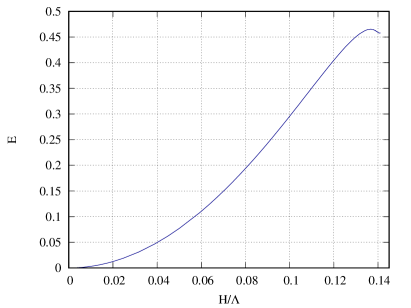
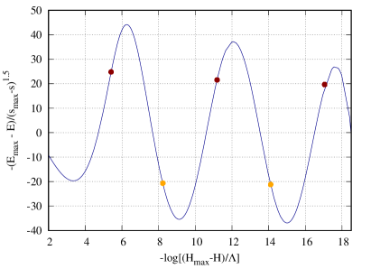
Figure 2: (Left Panel) The Hamiltonian, $E$, as a function of $s$, the steepness of the Stokes wave, exhibits oscillations in the vicinity of the limiting wave. (Right Panel) In order to distinguish the tiny features of oscillations we show a magnified plot in the logarithmic scale $-\log(s_{max}-s)$ and the Hamiltonian is magnified by a factor $(s_{max}-s)^{3/2}$. The extrema of the Hamiltonian are displaced to positions marked by the red points (the maxima) and the golden points (the minima).

It was shown in Tanaka (1983)-Longuet-Higgins and Tanaka (1997b) that as we increase steepness of the Stokes wave, after some threshold, there appears the first unstable eigenmode. It was investigated in details in the papers mentioned before. Also it was demonstrated that with further increase of stepness the second unstable mode appears. The values of steepness, which are thresholds for new unstable modes appearance, correspond to the local extrema of the Hamiltonian of the Stokes wave. We were able to investigate in details the first three unstable modes.

It is convenient to consider square of the eigenvalues corresponding to unstable modes as a function of steepness. Before the threshold eigenvalues are purely imaginary and above the threshold they are purely real. So we can define the threshold as a point where square of the eigenvalue goes through zero. Corresponding functions for the first two unstable modes are represented in Figure 3.

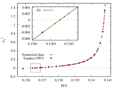
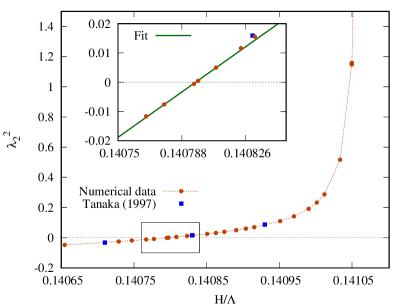
Figure 3: (Left) The square of first real eigenvalue $\lambda^{2}(s)$ is crossing the instability threshold at $s_{1}=0.1366035$ when Hamiltonian goes through the first local extremum. The eigenvalues computed in present work (orange circles), the numerical data of the work Longuet-Higgins and Tanaka (1997b) (blue squares) all fit well with the same line (green line); (Right) The square of the second real eigenvalue $\lambda^{2}(s)$ crosses the instability threshold at $s_{2}=0.140796$.

We used a least square fit to a linear function:

$$f_{n}(s)\sim(s-s_{n})$$ (23)

in the vicinity of appearance of every eigenmode. As a result of this procedure we were able to find thresholds for the appearance of the first unstable mode $s_{1}=0.136603552635709$ and the second mode $s_{2}=0.140796170578837$. These numbers correspond to the values obtained from direct Stokes waves calculations (see Table 1 up to 7 and 6 digits, respectively (close to accuracy of the obtained eigenvalues). For the third unstable eigenmode the fitting procedure gave $s_{3}=0.141049633798808$, 7 digits of which coincide with the result of direct computations in Table 1. The plot of squared eigenvalues is given in the left panel of Figure 4.

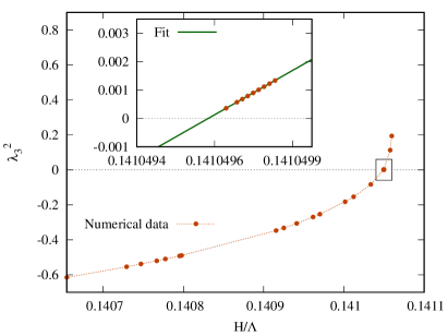
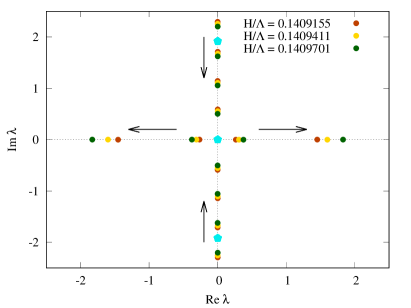
Figure 4: (Left) The square of the third real eigenvalue is crossing the instability threshold at $s_{3}=1.410496$ at the third local extremum of the Hamiltonian. Circles are numerical solutions of eigenvalue problem, and solid line is a numerical fit. (Right) A motion of eigenvalues near the origin just after the second extremum of the Hamiltonian, shows that there are two kinds of eigenvalues, the ones that are sensitive to small changes in $s$ (red, yellow and green), and the less sensitive ones (cyan). It is evident that more eigenvalues are moving to the origin to collide and produce more unstable eigenmodes.

III.1 Dependence of eigenvalues on the steepness and appearance of new branches of instability

In the right panel of Figure 4 one can observe that eigenvalues continuously move in the complex plane as steepness grows. We find that some eigenvalues are more sensitive than others to small changes of steepness of the underlying Stokes wave. The less sensitive eigenvalues are marked with cyan pentagons, they are located at the origin and on the imaginary axis.

The green, yellow and red circles correspond to the sensitive eigenvalues that are observed as complex conjugated pairs. These eigenvalues continuously move toward the origin as the steepness of the underlying Stokes wave grows. The first pair collides at the origin when the steepness of the underlying Stokes wave reaches the first maximum of the Hamiltonian, the second pair collides when the steepness of Stokes wave reaches the first minimum of the Hamiltonian, and so forth. The mechanism of collisions with formation of unstable modes was previously discussed in the work MacKay and Saffman (1986).

The linear dispersion relation of the gravity wave in the frame moving with velocity $c$ is given by $\omega_{k}=\pm ck\pm\sqrt{gk}$. It provides a good estimate to the eigenvalues for linearization about small amplitude Stokes waves, but we find that finite amplitude Stokes waves always have small deviations from the linear dispersion relation due to the nonlinear frequency shift Zakharov et al. (1992). The discrepancy between the linear dispersion and less sensitive eigenvalues obtained numerically become more evident as the steepness of the Stokes waves, hence nonlinearity of the system, grows.

III.2 Universal dependence of branches of instability

It is striking to note, that all computed eigenvalues for all eigemodes ($n=1,2,3$) collapse into one curve (see Figure 5, left panel). Here we used the normalized variable $(s_{max}-s)/(s_{max}-s_{n})$ on horizontal axis where $n=1,2,3$ is the number of the unstable eigenmode and $s_{max}$ corresponds to the steepness of the limiting Stokes wave (e.g. see Dyachenko et al. (2016)).

The curve is fitted by the nonlinear least squares algorithm to the function $(b_{0}+b_{1}x+b_{2}x^{2}+b_{3}x^{3})\log(x)$ with $b_{0}=-0.140023$, $b_{1}=0.0366936$, $b_{2}=-0.0129251$, and $b_{3}=0.00125835$. In the right panel of the Figure 5, we see that the eigenvalues can be well approximated by the power law $\lambda_{n}^{2}\propto 1/(s_{max}-s)$ in the vicinity of the limiting Stokes wave for all $n$.

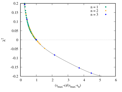
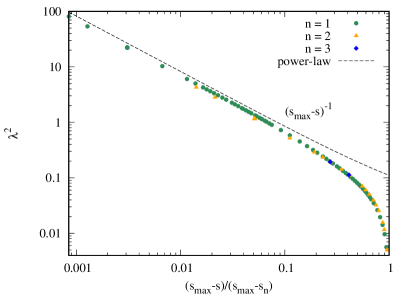
Figure 5: (Left panel) All eigenvalues corresponding to unstable eigenmodes collapse to a single universal curve as a function of normalized steepness $(s_{max}-s)/(s_{max}-s_{n})$, where $n=1,2,3$ is the number of the unstable eigenmode and $s_{max}$ corresponds to the steepness of the limiting Stokes wave. (Right panel) Plot in loglog scale of eigenvalues and power law $\lambda_{n}^{2}\sim 1/(s_{max}-s)$ in the vicinity of the limiting wave for all $n$.

IV Discussion and Conclusions

We compute the first three unstable eigenmodes of linearized equations about Stokes waves with the same spatial period as in Stokes wave (superharmonic instability). It is shown that these unstable modes emerge at the threshold values of steepness, which correspond to the extrema of Hamiltonian. This fact supports and extends observations in Longuet-Higgins and Tanaka (1997b). The results of numerical computations suggest that eigenvalues corresponding to unstable eigenmodes appear due to a collision of a pair of purely imaginary eigenvalues at the origin in the complex plane when steepness reaches the threshold values.

Our conjecture based on the results in the Figure 5 is that all eigenvalues corresponding to unstable eigenmodes above and below the thresholds of instability lie on a single curve if we plot them as a function of normalized steepness $(s_{max}-s)/(s_{max}-s_{n})$. In addition, our simulations suggest power law for $\lambda_{n}^{2}\sim 1/(s_{max}-s)$ in the vicinity of the limiting wave for unstable eigenmodes $n=1,2,3$. Further analytical work is needed to explain these observations.

Investigation of the stability properties can give one an insight into the evolution of the Stokes wave. In practice trains of Stokes waves in turbulent ocean is always accompanied by other small waves which can be considered as perturbation of the solution. If we can represent such perturbation as a combination of unstable eigenmodes, the initial stage of the dynamics of the perturbation will be determined by growth rates of the unstable eigenmodes.

The approach to investigation of instabilities of solutions similar to Stokes waves developed in this paper can be applied to study stability of Stokes waves with constant vorticity Dosaev et al. (2017); Murashige and Choi (2020). We plan to extend the stability analysis of the present paper to waves on a linear shear current formulated in conformal variables such see e.g. Dyachenko and Hur (2019).

Appendix A Auxiliary Conformal Mapping

We employ additional conformal mapping given by the formula:

$$u(q)=2\operatorname{atan}{L\tan{\frac{q}{2}}},\quad\mbox{and}\quad q_{u}=\frac{1}{L}\left(\cos^{2}{\frac{q}{2}}+L^{2}\sin^{2}{\frac{q}{2}}\right)$$ (24)

that allows to reduce the number of Fourier modes for resolving eigenfunctions of the linearization problem from $N$ to $\sim\sqrt{N}$ and allows to find eigenvalues in the vicinity of the third extremum of the Stokes wave.

The eigenvalue problem formulated in the $q$-plane is closely related to the equations (14) and is given by:

$$\lambda u_{q}\delta R_{1} =c(\delta R_{1})_{q}+\mathrm{i}\left[\delta U_{1}R_{q}+U(\delta R_{1})_{q}-\delta R_{1}U_{q}-R(\delta U_{1})_{q}\right],$$

$$\lambda u_{q}\delta\bar{R}_{2} =c(\delta\bar{R}_{2})_{q}-\mathrm{i}\left[\delta\bar{U}_{2}\bar{R}_{q}+\bar{U}(\delta\bar{R}_{2})_{q}-\delta\bar{R}_{2}\bar{U}_{q}-\bar{R}(\delta\bar{U}_{2})_{q}\right],$$ (25)

$$\lambda u_{q}\delta V_{1} =c(\delta V_{1})_{q}+\mathrm{i}\left[\delta U_{1}V_{q}+U(\delta V_{1})_{q}-\delta R_{1}B_{q}-R(\delta B_{1})_{q}\right]+gu_{q}\delta R_{1},$$

$$\lambda u_{q}\delta\bar{V}_{2} =c(\delta\bar{V}_{2})_{q}-\mathrm{i}\left[\delta\bar{U}_{2}\bar{V}_{q}+\bar{U}(\delta\bar{V}_{2})_{q}-\delta\bar{R}_{2}\bar{B}_{q}-\bar{R}(\delta\bar{B}_{2})_{q}\right]+gu_{q}\delta\bar{R}_{2},$$

References

- Stokes (1847) G. G. Stokes, Transactions of the Cambridge Philosophical Society 8, 441 (1847).
- Stokes (1880a) G. G. Stokes, Mathematical and Physical Papers 1, 197 (1880a).
- Stokes (1880b) G. G. Stokes, Mathematical and Physical Papers 1, 314 (1880b).
- Michell (1893) J. H. Michell, The London, Edinburgh, and Dublin Philosophical Magazine and Journal of Science 36, 430 (1893).
- Nekrasov (1921) A. I. Nekrasov, Izv. Ivanovo-Voznesensk. Polytech. Inst. 3, 52 (1921).
- Grant (1973) M. A. Grant, J. Fluid Mech. 59(2), 257 (1973).
- Schwartz (1974) L. W. Schwartz, J. Fluid Mech. 62(3), 553 (1974).
- Longuet-Higgins and Fox (1977) M. S. Longuet-Higgins and M. J. H. Fox, J. Fluid Mech. 80(4), 721 (1977).
- Longuet-Higgins and Fox (1978a) M. S. Longuet-Higgins and M. J. H. Fox, J. Fluid Mech. 85(4), 769 (1978a).
- Toland (1978) J. F. Toland, Proceedings of the Royal Society of London. A. Mathematical and Physical Sciences 363, 469 (1978).
- Plotnikov (1982) P. Plotnikov, Dinamika Splosh. Sredy (In Russian. English translation Stud. Appl. Math. 108:217-244 (2002)) 57, 41 (1982).
- Amick et al. (1982) C. J. Amick, L. E. Fraenkel, and J. F. Toland, Acta Math. 148, 193 (1982).
- Williams (1981) J. M. Williams, Phil. Trans. R. Soc. Lond. A 302(1466), 139 (1981).
- Williams (1985) J. M. Williams, Tables of Progressive Gravity Waves (Pitman, London, 1985).
- Tanveer (1991) S. Tanveer, Proc. R. Soc. Lond. A 435, 137 (1991).
- Longuet-Higgins (2008) M. S. Longuet-Higgins, Wave Motion 45, 770 (2008).
- Dyachenko et al. (2013) S. A. Dyachenko, P. M. Lushnikov, and A. O. Korotkevich, JETP Letters 98, 675 (2013).
- Dyachenko et al. (2016) S. A. Dyachenko, P. M. Lushnikov, and A. O. Korotkevich, Studies in Applied Mathematics 137, 419 (2016), eprint 1507.02784.
- Lushnikov (2016) P. M. Lushnikov, Journal of Fluid Mechanics 800, 557 (2016).
- Lushnikov et al. (2017) P. M. Lushnikov, S. A. Dyachenko, and D. A. Silantyev, Proc. Roy. Soc. A 473, 20170198 (2017).
- Longuet-Higgins (1978a) M. S. Longuet-Higgins, Proceedings of the Royal Society of London. A. Mathematical and Physical Sciences 360, 471 (1978a).
- Longuet-Higgins (1978b) M. S. Longuet-Higgins, Proceedings of the Royal Society of London. A. Mathematical and Physical Sciences 360, 489 (1978b).
- Benjamin and Feir (1967) T. B. Benjamin and J. E. Feir, J. Fluid mech 27, 417 (1967).
- Lighthill (1965) M. J. Lighthill, J. Inst. Maths. Applics. 1, 269 (1965).
- Whitham (1967) G. B. Whitham, Journal of Fluid Mechanics 27, 399 (1967).
- Zakharov (1968) V. E. Zakharov, J. Appl. Mech. Tech. Phys. 9, 190 (1968).
- Bespalov and Talanov (1966) V. I. Bespalov and V. I. Talanov, JETP Letters 3, 307 (1966).
- Zakharov and Ostrovsky (2009) V. E. Zakharov and L. A. Ostrovsky, Phys. D 540–548, 238 (2009).
- Deconinck and Oliveras (2011) B. Deconinck and K. Oliveras, Journal of Fluid Mechanics 675, 141 (2011).
- Creedon et al. (2022) R. P. Creedon, B. Deconinck, and O. Trichtchenko, Journal of Fluid Mechanics 937 (2022).
- Murashige and Choi (2020) S. Murashige and W. Choi, Journal of Fluid Mechanics 885 (2020).
- Banner and Tian (1998) M. L. Banner and X. Tian, J. Fluid Mech. 367, 107 (1998).
- Banner et al. (2000) M. L. Banner, A. V. Babanin, and I. R. Young, J. Phys. Oceanogr. 30, 3145 (2000).
- Song and Banner (2002) J.-B. Song and M. L. Banner, J. Phys. Oceanography 32, 2541 (2002).
- Korotkevich et al. (2019) A. O. Korotkevich, A. O. Prokofiev, and V. E. Zakharov, JETP Lett. 109, 309 (2019), eprint 1808.04953.
- Tanaka (1983) M. Tanaka, Journal of the physical society of Japan 52, 3047 (1983).
- Saffman (1985) P. Saffman, Journal of Fluid Mechanics 159, 169 (1985).
- Bridges (2004) T. J. Bridges, Journal of Fluid Mechanics 505, 153 (2004).
- Longuet-Higgins and Tanaka (1997a) M. Longuet-Higgins and M. Tanaka, J. Fluid Mech. 336, 51 (1997a).
- Longuet-Higgins and Cokelet (1978) M. S. Longuet-Higgins and E. D. Cokelet, Proceedings of the Royal Society of London. A. Mathematical and Physical Sciences 364, 1 (1978).
- Longuet-Higgins and Dommermuth (1997a) M. S. Longuet-Higgins and D. G. Dommermuth, Journal of Fluid Mechanics 33–50, 336 (1997a).
- Dyachenko and Newell (2016) S. Dyachenko and A. C. Newell, Studies in Applied Mathematics 137, 199 (2016).
- Ovsyannikov (1973) L. V. Ovsyannikov, M.A. Lavrent’ev Institute of Hydrodynamics Sib. Branch USSR Ac. Sci. 15, 104 (1973).
- Meison et al. (1981) D. Meison, S. Orzag, and M. Izraely, J. Comput. Phys. 40, 345 (1981).
- Tanveer (1993) S. Tanveer, Proc. R. Soc. Lond. A 441, 501 (1993).
- Dyachenko et al. (1996) A. I. Dyachenko, E. A. Kuznetsov, M. Spector, and V. E. Zakharov, Phys. Lett. A 221, 73 (1996).
- Chalikov and Sheinin (1998) D. Chalikov and D. Sheinin, Adv. Fluid Mech 17, 207 (1998).
- Chalikov and Sheinin (2005) D. Chalikov and D. Sheinin, Journal of Computational Physics 210, 247 (2005).
- Dyachenko (2001) A. I. Dyachenko, Dokl. Math. 63, 115 (2001).
- Dyachenko et al. (2022) S. A. Dyachenko, P. M. Lushnikov, A. O. Korotkevich, A. Semenova, and D. Silantyev (2022), URL http://stokeswave.org.
- ARPACK-NG (2020) ARPACK-NG (2020), URL https://github.com/opencollab/arpack-ng.
- Saad (1992) Y. Saad, Numerical methods for large eigenvalue problems (Manchester University Press, 1992).
- Saad and Schultz (1986) Y. Saad and M. H. Schultz, SIAM J. Sci. Stat. Comput. 7, 856 (1986).
- Longuet-Higgins and Fox (1978b) M. S. Longuet-Higgins and M. J. H. Fox, J. Fluid Mech. 85, 769 (1978b).
- Longuet-Higgins and Dommermuth (1997b) M. S. Longuet-Higgins and D. G. Dommermuth, Journal of Fluid Mechanics 336, 33 (1997b).
- Longuet-Higgins and Tanaka (1997b) M. Longuet-Higgins and M. Tanaka, Journal of Fluid Mechanics 336, 51 (1997b).
- MacKay and Saffman (1986) R. S. MacKay and P. G. Saffman, Proceedings of the Royal Society of London. A. Mathematical and Physical Sciences 406, 115 (1986).
- Zakharov et al. (1992) V. E. Zakharov, V. S. Lvov, and G. Falkovich, Kolmogorov Spectra of Turbulence I (Springer-Verlag, Berlin, 1992).
- Dosaev et al. (2017) A. S. Dosaev, Y. I. Troitskaya, and M. I. Shishina, Fluid Dynamics 52, 58 (2017).
- Dyachenko and Hur (2019) S. A. Dyachenko and V. M. Hur, Journal of Fluid Mechanics 878, 502 (2019).
- Frigo and Johnson (2005) M. Frigo and S. G. Johnson, Proc. IEEE 93, 216 (2005), URL http://fftw.org.
- GNU Project (1984-2021) GNU Project, http://gnu.org (1984-2021), URL http://gnu.org.