Effects of a Geometrically Realized Early Dark Energy Era on the Spectrum of Primordial Gravitational Waves

Abstract

In this work we investigate the effects of a geometrically generated early dark energy era on the energy spectrum of the primordial gravitational waves. The early dark energy era, which we choose it to have a constant equation of state parameter $w$, is synergistically generated by an appropriate $f(R)$ gravity in the presence of matter and radiation perfect fluids. As we demonstrate, the predicted signal for the energy spectrum of the $f(R)$ primordial gravitational waves is amplified and can be detectable, for various reheating temperatures, especially for large reheating temperatures. The signal amplitude depends on the duration of the early dark energy era and on the value of the dark energy equation of state parameter, with the most latter affecting more crucially the amplification. Specifically the amplification occurs when the equation of state parameter approaches the de Sitter value $w=-1$. Regarding the duration of the early dark energy era, we find that the largest amplification occurs when the early dark energy era commences at a temperature $T=0.85\,$eV until $T=7.8\,$eV. Moreover we study a similar scenario in which amplification occurs, where the early dark energy era commences at $T=0.29\,$eV and lasts until the temperature is increased by $\Delta T\sim 1.7\,$eV.

Introduction

One of the solutions proposed in the literature for solving the $H_{0}$-tension problem is the existence of an early dark energy era Niedermann:2020dwg ; Poulin:2018cxd ; Karwal:2016vyq ; Oikonomou:2020qah ; Nojiri:2019fft . If such an era is observed, then this could eliminate the $H_{0}$-tension problem. In this work the focus is on the effects of an early dark energy era on the energy spectrum of the primordial gravitational waves generated by an $f(R)$ gravity. Specifically we shall assume that an $f(R)$ gravity is the underlying geometric source that drives inflation, the early dark energy era and the late-time acceleration era, the commonly known dark energy era. In our approach, inflation will be controlled by a vacuum $R^{2}$ gravity, while the early and ordinary dark energy era will synergistically be controlled by appropriate $f(R)$ gravity terms and radiation and cold dark matter fluids. Our aim is to see in a quantitative way the direct effect of a geometrically generated early dark energy era on the primordial gravitational waves energy spectrum. For our analysis, we shall use the theoretically predicted energy spectrum, which appears in many studies, see for example Refs. Kamionkowski:2015yta ; Denissenya:2018mqs ; Turner:1993vb ; Boyle:2005se ; Zhang:2005nw ; Schutz:2010xm ; Sathyaprakash:2009xs ; Caprini:2018mtu ; Arutyunov:2016kve ; Kuroyanagi:2008ye ; Clarke:2020bil ; Kuroyanagi:2014nba ; Nakayama:2009ce ; Smith:2005mm ; Giovannini:2008tm ; Liu:2015psa ; Zhao:2013bba ; Vagnozzi:2020gtf ; Watanabe:2006qe ; Kamionkowski:1993fg ; Giare:2020vss ; Kuroyanagi:2020sfw ; Zhao:2006mm ; Nishizawa:2017nef ; Arai:2017hxj ; Bellini:2014fua ; Nunes:2018zot ; DAgostino:2019hvh ; Mitra:2020vzq ; Kuroyanagi:2011fy ; Campeti:2020xwn ; Nishizawa:2014zra ; Zhao:2006eb ; Cheng:2021nyo ; Nishizawa:2011eq ; Chongchitnan:2006pe ; Lasky:2015lej ; Guzzetti:2016mkm ; Ben-Dayan:2019gll ; Nakayama:2008wy ; Capozziello:2017vdi ; Capozziello:2008fn ; Capozziello:2008rq ; Cai:2021uup ; Cai:2018dig ; Odintsov:2021kup ; Benetti:2021uea ; Lin:2021vwc ; Zhang:2021vak ; Odintsov:2021urx ; Pritchard:2004qp ; Zhang:2005nv ; Baskaran:2006qs ; Oikonomou:2022xoq ; Odintsov:2022cbm ; Odintsov:2022sdk and references therein, and we shall evaluate numerically the effects of the $f(R)$ gravity on the general relativistic waveform. We shall use a WKB approach developed in Nishizawa:2017nef and we shall investigate the amount of amplification caused by an early dark energy era, which is generated by an $f(R)$ gravity in the presence of perfect matter and radiation fluids. The early dark energy era is described by a constant equation of state (EoS) parameter $w$, and we shall find which $f(R)$ gravity can generate such an evolution in the presence of matter and radiation perfect fluids. Then we shall calculate the overall amplification factor of the general relativistic energy spectrum of the primordial gravitational waves. Our results will be confronted with the sensitivity curves of future interferometric experiments, like the LISA laser interferometer space antenna Baker:2019nia ; Smith:2019wny , the DECIGO Seto:2001qf ; Kawamura:2020pcg , the Einstein Telescope Hild:2010id , the future BBO (Big Bang Observatory) Crowder:2005nr ; Smith:2016jqs , and also the non-interferometric experiments Square Kilometer Array (SKA) Bull:2018lat and the NANOGrav collaboration Arzoumanian:2020vkk ; Pol:2020igl . As we shall demonstrate, the general relativistic energy spectrum is amplified by the presence of an $f(R)$ gravity generated early dark energy era, only if several conditions hold true. Specifically, the duration of the early dark energy era plays an important role and also the value of the EoS parameter $w$ also crucially affects the results. As we show, in most of the cases we studied, the energy spectrum signal is amplified due to this $f(R)$ gravity generated early dark energy era. As a conclusion, we point out that a detection of a stochastic gravitational wave signal in future interferometric experiments may have many possible explanations, and the early dark energy realized by an f(R) gravity is one of these explanations.

I $f(R)$ Gravity Realization of Inflation and Subsequent Eras

The standard approach for realizing various cosmological eras in Einstein-Hilbert cosmology is usually done by using perfect matter fluids. The latter dominate the evolution at certain point, and the corresponding era is controlled by those fluids, for example the radiation domination era is controlled by the radiation fluid, the energy density of which redshifts as $\rho_{r}\sim a^{-4}$, where $a$ is the scale factor of a flat Friedmann-Robertson-Walker (FRW) metric. Also for the matter domination era the matter perfect fluid dominates the evolution, which describes non-baryonic non-relativistic matter and its energy density redshifts as $\rho_{m}\sim a^{-3}$. Apart from the three standard evolution eras which we usually assume that the Universe underwent, that is, the inflationary, radiation and matter domination and dark energy era, we basically do not know the behavior of our Universe post-inflationary. We have hints for the post-inflationary era, but no proofs. This era is a mysterious era, and it commences with the reheating era, which is the beginning of radiation era, and it is believed that the reheating era smoothly deforms to the radiation era. Remarkably, we also lack of knowledge of what happened from the reheating era up to the matter domination era, and before the recombination era. So the question is what do we know? We know very well the physics beyond the recombination era, up to the present day. The recombination era is basically where the last scattering surface of the CMB photons was formed, and from this era until present day we understand the physics relatively well.

Thus the epoch before the recombination era we have no measured data from that era, only at last scattering and beyond. So let us assume that an early dark energy era is realized before the recombination and specifically from the matter-radiation equality redshift $z\sim 3400$ until some final redshift in the past, deeply in the matter domination era $z_{f}$. In this work we shall assume that this final redshift is a free variable and we shall investigate what would be the effect of an early dark energy era on the spectrum of the primordial gravitational waves, focusing on modes which were subhorizon modes immediately after the inflationary era and during the first stages of the reheating era. Also, regarding the early dark energy era itself, we shall assume that it is described by a constant EoS parameter, and more importantly, it is not realized by some perfect matter fluid, but it is realized geometrically, by some dominant form of $f(R)$ gravity for the whole early dark energy era. Also it is natural to assume that $f(R)$ controls the inflationary and the late dark energy era, as follows,

$$f(R)=\left\{\begin{array}[]{ccc}R+\frac{R^{2}}{6M^{2}}&R\sim R_{I}\,,\\ F_{w}(R)&R_{f}\leq R\ll R_{eq}\,,\\ R+F_{DE}(R)&R\sim R_{0}\ll R_{rec}\,,\\ \end{array}\right.$$

with $R_{I}$ being the curvature scale of inflation, which is calculated primordially when the modes exit the horizon at the first time, so at the beginning of inflation. Also the curvature scale $R_{rec}$ is the curvature scale at the recombination, $R_{f}$ is the curvature scale when the early dark energy era commences, $R_{eq}$ the curvature at matter radiation equality and $R_{0}$ is the curvature scale at present day, so it is basically identical with the cosmological constant. Note that according to our scenario, the era between the curvature scales $R_{I}<R<R_{f}$ is not described by modified gravity. So modified gravity affects post-inflationary the evolution after $R>R_{f}$.

The exact forms of $F_{w}(R)$ and $F_{DE}(R)$ will be specified shortly on the basis of phenomenological viability. Regarding the function $F_{w}(R)$, this in conjunction with the matter and radiation perfect fluids will synergistically generate the early dark energy era with a constant EoS parameter $w$, and we shall find that shortly. The function $F_{DE}(R)$ will realize the dark energy era, at late-times, so some appropriate form of this will be used in order to provide a viable dark energy era phenomenology. In order to find the exact forms of the $f(R)$ gravity, we consider the gravitational action with perfect matter fluids present,

$$\mathcal{S}=\frac{1}{2\kappa^{2}}\int\mathrm{d}^{4}x\sqrt{-g}\,f(R)+\mathcal{S}_{m}\,,$$ (1)

with $\kappa^{2}=8\pi G=\frac{1}{M_{p}^{2}}$, with being $G$ Newton’s constant, and $M_{p}$ stands for the reduced Planck mass. In the metric formalism, the field equations are,

$$f_{R}(R)R_{\mu\nu}(g)-\frac{1}{2}f(R)g_{\mu\nu}-\nabla_{\mu}\nabla_{\nu}f_{R}(R)+g_{\mu\nu}\square f_{R}(R)=\kappa^{2}T_{\mu\nu}^{m}\,,$$ (2)

with $T_{\mu\nu}^{m}$ being the energy momentum tensor of the matter and radiation perfect fluids, and furthermore $f_{R}=\frac{\mathrm{d}f}{\mathrm{d}R}$. For a flat FRW spacetime, in which case the line element reads,

$$\centering{\rm d}s^{2}=-{\rm d}t^{2}+a(t)^{2}\sum_{i=1}^{3}{({\rm d}x^{i})^{2}}\,,\@add@centering$$ (3)

the field equations become,

$$-18\left(4H(t)^{2}\dot{H}(t)+H(t)\ddot{H}(t)\right)f_{RR}(R)+3\left(H^{2}(t)+\dot{H}(t)\right)f_{R}(R)-\frac{f(R)}{2}+\kappa^{2}\left(\rho_{m}+\rho_{r}\right)=0\,,$$ (4)

with $\rho_{m}$, $\rho_{r}$ standing for the cold dark matter energy density and radiation energy density respectively.

Now let us proceed to the core of our analysis and we assume that the Universe goes through an intermediate early dark energy era, with a constant EoS parameter $w$, thus $p_{eff}=w\rho_{eff}$, where $p_{eff}$ and $\rho_{eff}$ are the Universe’s total pressure and energy density. The early dark energy era will be assumed to last from $z=3400$, so from the matter radiation equality, until a redshift $z_{f}$ which will be a free parameter in our analysis. During the early dark energy era, lasting from $z=3400$ up to $z=z_{f}$, the scale factor of the Universe is,

$$a(t)=a_{end}\,t^{\frac{2}{3(1+w)}}\,,$$ (5)

with $a_{end}$ being the scale factor at the redshift $z=z_{f}$. It is easy to find which geometrical $f(R)$ theory can realize the cosmology (5) synergistically in the presence of matter and radiation perfect fluids. In order to do so we shall apply the formalism of Ref. Nojiri:2009kx , so we use the $e$-foldings number as a dynamical variable, so we have,

$$e^{-N}=\frac{a_{i}}{a}\,,$$ (6)

where $a_{i}$ is some initial value of the scale factor. Using the $e$-foldings number $N$, the Friedmann equation takes the form,

$$-18\left[4H^{3}(N)H^{\prime}(N)+H^{2}(N)(H^{\prime})^{2}+H^{3}(N)H^{\prime\prime}(N)\right]f_{RR}(R)+3\left[H^{2}(N)+H(N)H^{\prime}(N)\right]f_{R}(R)-\frac{f(R)}{2}+\kappa^{2}\rho=0\,,$$ (7)

where $\rho=\rho_{m}+\rho_{r}$. Introducing the auxiliary function, $G(N)=H^{2}(N)$, the Ricci scalar is written as follows,

$$R=3G^{\prime}(N)+12G(N)\,.$$ (8)

Eventually the Friedman equation becomes,

$$-9G(N(R))\left[4G^{\prime}(N(R))+G^{\prime\prime}(N(R))\right]f_{RR}(R)+\left[3G(N)+\frac{3}{2}G^{\prime}(N(R))\right]f_{R}(R)-\frac{f(R)}{2}+\kappa^{2}\left(\rho_{m}+\rho_{r}\right)=0\,,$$ (9)

where $G^{\prime}(N)=\mathrm{d}G(N)/\mathrm{d}N$ and $G^{\prime\prime}(N)=\mathrm{d}^{2}G(N)/\mathrm{d}N^{2}$. By solving the above equation, one obtains the $f(R)$ gravity which realizes the given scale factor of interest, which in our case is that of Eq. (5). Let us now proceed to find the explicit form of the $f(R)$ gravity which realizes the scale factor (5). For the scale factor (5), $G(N)$ becomes,

$$G(N)=\frac{4e^{-3N(w+1)}}{9(w+1)^{2}}\,,$$ (10)

and we took $a_{r}=1$ for simplicity. Upon combining Eqs. (8) and (10), we get,

$$N=\frac{\log\left(\frac{4(1-3w)}{3R(w+1)^{2}}\right)}{3(w+1)}.$$ (11)

The above in conjunction with the following,

$$\rho_{tot}=\sum_{i}\rho_{i0}a_{0}^{-3(1+w_{i})}e^{-3N(R)(1+w_{i})}\,,$$ (12)

affect the Friedmann equation (9), which becomes,

$$a_{1}R^{2}\frac{\mathrm{d}^{2}f(R)}{\mathrm{d}R^{2}}+a_{2}R\frac{\mathrm{d}f(R)}{\mathrm{d}R}-\frac{f(R)}{2}+\sum_{i}S_{i}R^{\frac{3(1+w_{i})}{3(1+w)}}=0\,,$$ (13)

where the index “i” takes values $i=(r,m)$ with $i=r$ indicating radiation and $i=m$ indicating cold dark matter perfect fluids. Also the parameters $a_{1}$ and $a_{2}$, $S_{i}$ and $A$ are defined in the following way,

$$a_{1}=\frac{3(1+w)}{4-3(1+w)},\,\,\,a_{2}=\frac{2-3(1+w)}{2(4-3(1+w))},\,\,\,S_{i}=\frac{\kappa^{2}\rho_{i0}a_{0}^{-3(1+w_{i})}}{[3A(4-3(1+w))]^{\frac{3(1+w_{i})}{3(1+w)}}},\,\,\,A=\frac{4}{3(w+1)}$$ (14)

By solving (13) we will get the $f(R)$ gravity which generates the early dark energy era, which was denoted $F_{w}(R)$ previously, so the solution is,

$$F_{w}(R)=\left[\frac{c_{2}\rho_{1}}{\rho_{2}}-\frac{c_{1}\rho_{1}}{\rho_{2}(\rho_{2}-\rho_{1}+1)}\right]R^{\rho_{2}+1}+\sum_{i}\left[\frac{c_{1}S_{i}}{\rho_{2}(\delta_{i}+2+\rho_{2}-\rho_{1})}\right]R^{\delta_{i}+2+\rho_{2}}-\sum_{i}B_{i}c_{2}R^{\delta_{i}+\rho_{2}}+c_{1}R^{\rho_{1}}+c_{2}R^{\rho_{2}}\,,$$ (15)

where $c_{1},c_{2}$ are simple integration constants, and also $\delta_{i}$ and $B_{i}$ are,

$$\delta_{i}=\frac{3(1+w_{i})-23(1+w)}{3(1+w)}-\rho_{2}+2,\,\,\,B_{i}=\frac{S_{i}}{\rho_{2}\delta_{i}}\,,$$ (16)

with $i=(r,m)$. Let us now specify the late time era, and we shall choose a convenient $f(R)$ gravity which is known to provide a viable late-time phenomenology. We shall choose the one used in Ref. Odintsov:2021kup which is known to be a viable dark energy $f(R)$ gravity model, which is,

$$F_{DE}(R)=-\gamma\Lambda\Big{(}\frac{R}{3m_{s}^{2}}\Big{)}^{\delta}\,,$$ (17)

where $m_{s}$ is $m_{s}^{2}=\frac{\kappa^{2}\rho_{m}^{(0)}}{3}$, and also $\rho_{m}^{(0)}$ denotes the cold dark matter energy density at present day. Furthermore, the parameter $\delta$ is chosen $0<\delta<1$, $\gamma$ is an arbitrary dimensionless parameter, and $\Lambda$ is the cosmological constant. Hence, the Universe’s evolution is controlled during inflation by an $R^{2}$ model, while from $z_{f}$ and up to $z=3400$ by $F_{w}(R)$ given in Eq. (15), and at late times by $F_{DE}(R)$ given in Eq. (17). In principle it is not hard to find such a phenomenological model, for example such a phenomenological model would look like,

$$f(R)=e^{-\frac{\Lambda}{R}}\left(R+\frac{R^{2}}{6M^{2}}\right)+e^{-\frac{R}{\Lambda}}\tanh\left(\frac{R-R_{f}}{\Lambda}\right)\left(\frac{R-R_{eq}}{\Lambda}\right)F_{DE}(R)+e^{-\frac{R}{\Lambda}}\tanh\left(\frac{R-R_{0}}{\Lambda}\right)\left(F_{w}(R)-R-\frac{R^{2}}{6M^{2}}\right)\,.$$ (18)

It should be noted that the above model is not the only one that can reproduce the phenomenology we want to describe, it is one example, but certainly not the only one. We just quote one example for completeness. With regard to the early dark energy era we shall consider three cases for values of the EoS parameter, described below,

$$\mathrm{Scenario}\,\,I\,:\,\,\mathrm{EoS}\,\,w=-0.99\,\,\,,$$ (19)

$$\mathrm{Scenario}\,\,II\,:\,\,\mathrm{EoS}\,\,w=-\frac{1}{3}-0.001\,.,$$

$$\mathrm{Scenario}\,\,III\,:\,\,\mathrm{EoS}\,\,w=-0.7\,.$$

So Scenarios I and II basically describe the limiting cases of accelerating expansion nearly a de Sitter one (Scenario I) and nearly accelerating (Scenario II slightly smaller EoS parameter compared to the value of the EoS parameter for which non-accelerating nor decelerating cosmology occurs, namely $w=-\frac{1}{3}$). Finally, for Scenario III the EoS parameter takes an intermediate value for the sake of completeness.

Let us now proceed to the evaluation of the observational indices relevant to the calculation of the energy spectrum of the primordial gravitational waves. Specifically, we shall calculate the tensor-to-scalar ratio and the tensor spectral index. We shall be interested in modes with , which is the pivot scale used in Planck. For $f(R)$ gravity, the tensor spectral index is reviews1 ; Odintsov:2020thl ; Odintsov:2021kup ,

$$n_{T}\simeq-2\epsilon_{1}^{2}\,,$$ (20)

and the tensor-to-scalar ratio is reviews1 ; Odintsov:2020thl ; Odintsov:2021kup ,

$$r=48\epsilon_{1}^{2}\,,$$ (21)

with $\epsilon_{1}$ being the first slow-roll index $\epsilon_{1}=-\dot{H}/H^{2}$. For the $R^{2}$ gravity we have $\epsilon_{1}\simeq\frac{1}{2N}$, hence,

$$n_{T}\simeq-\frac{1}{2N^{2}}\,,$$ (22)

and the corresponding tensor-to-scalar ratio is,

$$r=\frac{12}{N^{2}}\,.$$ (23)

In the next section we shall evaluate numerically the energy spectrum of the primordial gravitational waves at present day, for all the modes that became subhorizon during the early stages of the reheating era. We shall be interested in short wavelength modes with $\lambda\gg 10\,$Mpc, or equivalently with wavenumbers $k>10^{7}\,$Mpc^-1 up to $k>10^{18}\,$Mpc^-1, which corresponds to the frequency range $10^{-7}<f<10^{3}\,$Hz.

II Primordial Gravitational Wave Energy Spectrum: The effects of an Early Dark Energy Phase

In the next ten years, several space interferometers will provide observational data on whether the theoretically predicted stochastic gravitational wave background exists or not. Already in the literature, the theoretical predictions for the stochastic background of primordial gravitational waves are intensively studied, see Refs. Kamionkowski:2015yta ; Denissenya:2018mqs ; Turner:1993vb ; Boyle:2005se ; Zhang:2005nw ; Schutz:2010xm ; Sathyaprakash:2009xs ; Caprini:2018mtu ; Arutyunov:2016kve ; Kuroyanagi:2008ye ; Clarke:2020bil ; Kuroyanagi:2014nba ; Nakayama:2009ce ; Smith:2005mm ; Giovannini:2008tm ; Liu:2015psa ; Zhao:2013bba ; Vagnozzi:2020gtf ; Watanabe:2006qe ; Kamionkowski:1993fg ; Giare:2020vss ; Kuroyanagi:2020sfw ; Zhao:2006mm ; Nishizawa:2017nef ; Arai:2017hxj ; Bellini:2014fua ; Nunes:2018zot ; DAgostino:2019hvh ; Mitra:2020vzq ; Kuroyanagi:2011fy ; Campeti:2020xwn ; Nishizawa:2014zra ; Zhao:2006eb ; Cheng:2021nyo ; Nishizawa:2011eq ; Chongchitnan:2006pe ; Lasky:2015lej ; Guzzetti:2016mkm ; Ben-Dayan:2019gll ; Nakayama:2008wy ; Capozziello:2017vdi ; Capozziello:2008fn ; Capozziello:2008rq ; Cai:2021uup ; Cai:2018dig ; Odintsov:2021kup ; Benetti:2021uea ; Lin:2021vwc ; Zhang:2021vak ; Odintsov:2021urx ; Pritchard:2004qp ; Zhang:2005nv ; Baskaran:2006qs ; Oikonomou:2022xoq ; Odintsov:2022cbm ; Odintsov:2022sdk and references therein.

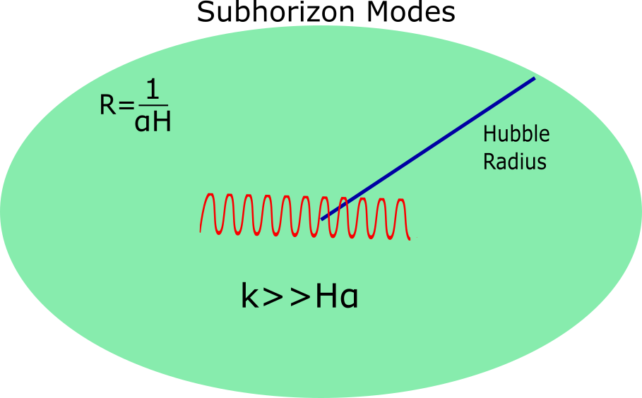
Figure 1: Subhorizon inflationary modes which during the inflationary era, these were at subhorizon scales, and have the smallest wavelength. These are the first that reenter the horizon after the end of the inflationary era and during the early stages of the reheating era. The subhorizon modes will be probed by future space interferometers.

In this paper, the focus is to investigate the effect of an $f(R)$ gravity realized early dark energy era, with constant EoS parameter $w$, which commences at the matter-radiation equality and stretches up to a final redshift $z_{f}$, which shall be a free variable for the moment. Our main assumption is that $z_{f}\sim\mathcal{O}(10^{4})$, but we shall allow for other higher values for completeness, in order to see the effect on the energy spectrum of the primordial gravitational waves. Let us note that the choice of $z_{f}$ is arbitrary, it just indicates the end of the early dark energy era. This is the maximum redshift which we will allow the upper redshift limit of the early dark energy era to be.

Let us discuss more the duration of the early dark energy era, and as we stated we shall assume that it starts around the matter-radiation equality at redshift $z=3400$ so at a temperature $T=0.85\,$eV Garcia-Bellido:1999qrp and it ends at $z_{f}$ which will be assumed in the range $z_{f}=[10^{4},3\times 10^{4}]$ which corresponds to a temperature range $T_{f}=[0.89,7.8]\,$eV Garcia-Bellido:1999qrp . In terms of the temperature, the early dark energy era does not go deeply in the radiation domination era, and specifically we shall assume that it lasts from $T=0.89\,$eV up to $T_{f}=2.6\,$eV, however we shall extend the duration up to $T_{f}=7.8\,$eV.

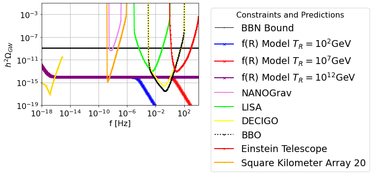
Figure 2: The $h^{2}$-scaled gravitational wave energy spectrum for the early dark energy $w$-era generated by $f(R)$ gravity, for the Scenario I for $z_{f}=10^{5}$, with reheating temperatures $T_{R}=10^{12}$GeV (purple), to $T_{R}=10^{7}$GeV (red) and to (blue) $T_{R}=10^{2}$GeV.

The procedure to extract the overall effect of the $f(R)$ gravity on the primordial gravitational waves is based on a WKB method which applies on the modes that became subhorizon just after the inflationary era ended, so during the reheating era. For a pictorial representation of the subhorizon modes see Fig. 1. The WKB method was developed in Refs. Nishizawa:2017nef ; Arai:2017hxj and relies on the calculation of the parameter $\alpha_{M}$, defined as,

$$a_{M}=\frac{f_{RR}\dot{R}}{f_{R}H}\,,$$ (24)

and the modified gravity effect on the waveform is,

$$h=e^{-\mathcal{D}}h_{GR}\,,$$ (25)

where $h_{GR}$ is the waveform with $a_{M}=0$ which corresponds to the general relativity case, and also the quantity $\mathcal{D}$ is defined as,

$$\mathcal{D}=\frac{1}{2}\int^{\tau}a_{M}\mathcal{H}{\rm d}\tau_{1}=\frac{1}{2}\int_{0}^{z}\frac{a_{M}}{1+z^{\prime}}{\rm dz^{\prime}}\,.$$ (26)

The primordial gravity waves energy density including the $f(R)$ gravity effects is Boyle:2005se ; Nishizawa:2017nef ; Arai:2017hxj ; Nunes:2018zot ; Liu:2015psa ; Zhao:2013bba ; Odintsov:2021kup ,

$$\Omega_{\rm gw}(f)=e^{-2\mathcal{D}}\times\frac{k^{2}}{12H_{0}^{2}}r\mathcal{P}_{\zeta}(k_{ref})\left(\frac{k}{k_{ref}}\right)^{n_{T}}\left(\frac{\Omega_{m}}{\Omega_{\Lambda}}\right)^{2}\left(\frac{g_{*}(T_{\rm in})}{g_{*0}}\right)\left(\frac{g_{*s0}}{g_{*s}(T_{\rm in})}\right)^{4/3}\left(\overline{\frac{3j_{1}(k\tau_{0})}{k\tau_{0}}}\right)^{2}T_{1}^{2}\left(x_{\rm eq}\right)T_{2}^{2}\left(x_{R}\right)\,,$$ (27)

with $k_{ref}=0.002$ Mpc^-1 being CMB pivot scale. Also $n_{T}$ denotes the tensor spectral index and $r$ denotes the tensor-to-scalar ratio. The calculation of the quantity $\mathcal{D}$ is the main aim hereafter, for the redshift ranges $z=[0,3400]$, and $z=[3400,3\times 10^{4}]$ and to see the overall amplification or damping on the energy spectrum. Thus the quantity that needs to be calculated is,

$$\mathcal{D}=\frac{1}{2}\left(\int_{0}^{3400}\frac{a_{M_{1}}}{1+z^{\prime}}{\rm dz^{\prime}}+\int_{3400}^{z_{f}}\frac{a_{M_{2}}}{1+z^{\prime}}{\rm dz^{\prime}}\right)\,,$$ (28)

with $a_{M_{1}}$ and $a_{M_{2}}$ being calculated for $f(R)\sim R+f_{DE}(R)$ and $f(R)\sim F_{w}(R)$ respectively and with $z_{f}$ varying in the range $z_{f}=[10^{4},3\times 10^{4}]$. Let us now present our analysis for the three different scenarios we defined in the previous section. For the scenarios II and III, the overall amplification factors $\mathcal{D}$ are nearly zero, hence the predicted energy spectrum of the primordial gravitational waves is undetectable. Just for the sake of being precise, for scenario II, the parameter $\mathcal{D}$ is $\mathcal{D}\sim 10^{-68}$ and these results apply for both the redshift ranges $z=[3400,10^{4}]$ and $z=[3400,3\times 10^{4}]$. Also the first integral $\frac{1}{2}\left(\int_{0}^{3400}\frac{a_{M_{1}}}{1+z^{\prime}}{\rm dz^{\prime}}\right)$ for all scenarios is of the order $\sim-0.05$ for all the scenarios. The only non-trivial result occurs only for the Scenario I, in which case we get $\int_{3400}^{10^{4}}\frac{a_{M_{2}}}{1+z^{\prime}}{\rm dz^{\prime}}=-4.6353$ and $\int_{3400}^{3\times 10^{4}}\frac{a_{M_{2}}}{1+z^{\prime}}{\rm dz^{\prime}}=-9.35798$, so in both cases amplification occurs for the energy spectrum. In Fig. 2 and 3 we plot the $f(R)$ gravity $h^{2}$-scaled energy spectrum as a function of the frequency, and specifically Fig. 2 corresponds to the case for which the early dark energy era lasts up to $z_{f}=10^{4}$ and Fig. 3 for $z_{f}=3\times 10^{4}$. In both the plots we also included the sensitivity curves of most of the future interferometer experiments, and the predicted energy spectrum is presented for three distinct reheating temperatures, for $T_{R}=10^{12}$GeV (purple curve), for $T_{R}=10^{7}$GeV (red curve) and $T_{R}=10^{2}$GeV (blue curve).

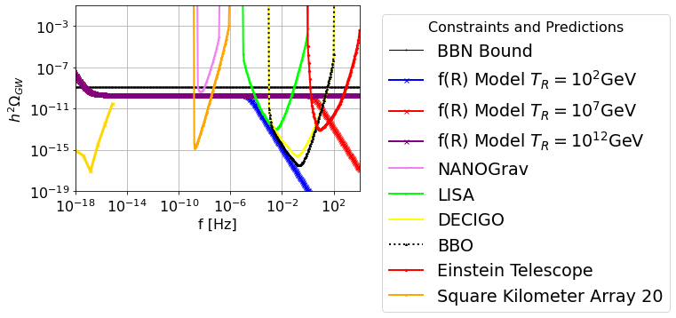
Figure 3: The $h^{2}$-scaled gravitational wave energy spectrum for the early dark energy $w$-era generated by $f(R)$ gravity, for the Scenario I for $z_{f}=3\times 10^{4}$, with reheating temperatures $T_{R}=10^{12}$GeV (purple), to $T_{R}=10^{7}$GeV (red) and to (blue) $T_{R}=10^{2}$GeV.

As it is obvious from both Figs. 2 and 3, the signals corresponding to the $f(R)$ gravity models are detectable from most future experiments. Specifically, for the case with $z_{f}=10^{4}$, the $f(R)$ gravity signal will be detected by the SKA experiment for all reheating temperatures, and by the DECIGO and BBO experiments for reheating temperatures $T_{R}=10^{7}$GeV and $T_{R}=10^{12}$GeV. As for the case with $z_{f}=3\times 10^{4}$, in which case the early dark energy era lasts slightly longer compared to the standard scenarios in the literature, the signal will be detected by all the experiments, except for the case with reheating temperature $T_{R}=10^{2}$GeV, which will be detected only by the SKA and NANOGrav experiments. Also let us note that if the early dark energy era commences earlier, for example at the recombination with $z\sim 1100$ and lasts until $z=10^{4}$, similar results are obtained. Indeed in this case we get $\int_{1100}^{10^{4}}\frac{a_{M_{2}}}{1+z^{\prime}}{\rm dz^{\prime}}=-10$, and in Fig. 4 we plot the $h^{2}$-scaled energy spectrum for this case. As it can be seen the signal will be detected by all the future experiments, except for the low reheating temperature scenario. As an overall comment for all the cases we studied in this section, it seems that the signal of $f(R)$ gravity gravitational waves depends on the duration of the early dark energy era, and for a good possibility of detection, the eras between which the early dark energy era occurs must have a temperature difference of approximately of the order $\Delta T\sim 1.7\,$eV. Also we need to comment on an important issue: since our WKB approach affects the subhorizon modes during reheating, the figures we presented must be looked with caution for small frequencies, because these modes were superhorizon during reheating. Hence our results are valid for frequencies starting from the NANOGrav until the Einstein telescope.

Figure 4: The $h^{2}$-scaled gravitational wave energy spectrum for the early dark energy $w$-era generated by $f(R)$ gravity, for the Scenario I for $z_{f}=\times 10^{4}$ and for starting redshift of the early dark energy era $z=1100$, with reheating temperatures $T_{R}=10^{12}$GeV (purple), to $T_{R}=10^{7}$GeV (red) and to (blue) $T_{R}=10^{2}$GeV.

Before closing this section, an important comment is in order. In standard contexts of the Starobinsky inflationary scenario, the signal of the primordial gravitational waves is undetectable. This has to do with the fact that the tensor spectral index for the standard Starobinsky inflation is negative, and thus, the energy spectrum of the primordial gravitational waves generated is significantly lower than the sensitivity curves of most future gravitational waves experiments. This result however is mainly based on a standard post-inflationary evolution, which includes the reheating, radiation domination and matter domination eras. However, with this work we aimed to show in a quantitative way that a geometrically generated early dark energy era which occurs just before recombination can amplify the energy spectrum significantly. By geometrically generated, we mean that the origin of this era is an $f(R)$ gravity in the presence of matter and radiation perfect fluids. The reason for this amplification is an overall amplifying factor $\sim e^{-2\mathcal{D}}$ appearing in front of Eq. (27). This factor takes into account the WKB effects of the modified gravity beyond the inflationary era. The gravitational waves still redshift as radiation but their energy spectrum is amplified, and this amplification is a direct modified gravity effect, due to the fact that the evolution equation contains a WKB overall factor. In most studies known for the Starobinsky inflation predictions for primordial gravitational waves, this post-inflationary amplification is absent, due to the fact that the post-inflationary evolution is comprised by the reheating, radiation domination and matter domination eras. In our case, post-inflationary there are non-trivial effects generated by the $f(R)$ gravity geometrically generated early dark energy era. To show in a simple and brief way this issue, in the presence of a non-trivial modified gravity, the evolution equation for tensor perturbations is described by the following equation, of the tensor perturbation $h_{ij}$,

$$\ddot{h}(k)+\left(3+a_{M}\right)H\dot{h}(k)+\frac{k^{2}}{a^{2}}h(k)=0\,,$$ (29)

where $\alpha_{M}$ is in our case given in Eq. (24). If post-inflationary the evolution is the standard one, then the solution to the above equation is described by the one appearing in Eq. (25) without the factor $\sim e^{-\mathcal{D}}$, thus $h(k)\sim h_{GR}$. In our case though, the amplifying factor is non-trivial and as we showed numerically by evaluating $\mathcal{D}$ in Eq. (26) for a constant EoS parameter early dark energy era generated by $f(R)$ gravity in the presence of matter and radiation perfect fluids, the amplification is significant.

Furthermore, we need to clarify that the epochs before the early dark energy era are not affected at all in our framework. The only effect of the early dark energy era is contained in the amplifying factor $\mathcal{D}$ in Eq. (27). The post-inflationary epochs in between inflation and the early dark energy era are contained in the Eq. (27), and even the era of BBN is contained there. The BBN bounds are also taken into consideration in Figs. 2-4, corresponding to a straight solid black line.

III Conclusions

In this work we investigated quantitatively the effect of a geometrically generated early dark energy era on the energy spectrum of the primordial gravitations waves. Specifically the early dark energy era is generated by an appropriate $f(R)$ gravity in the presence of matter and radiation perfect fluids. The main assumption we made is that $f(R)$ gravity generates the inflationary era, and specifically an $R^{2}$ gravity, the late-time acceleration era, and also the early dark energy era. As we showed, the energy spectrum of the primordial gravitational waves is significantly amplified in a detectable way, and the signal can be detected by most of the future gravitational waves experiments that will seek for stochastic gravitational waves. Our analysis indicated that the amplification of the signal depends on two crucial parameters, the value of the dark energy EoS parameter $w$ and the duration of the early dark energy era. As we showed, the amplification occurs only when the EoS parameter of the early dark energy era is close to the de Sitter value and specifically we studied the case $w=-0.9$. In addition the duration of the early dark energy era affects the amplification. We assumed that the early dark energy era started at $z=3400$ up to $z=3\times 10^{4}$ and also we considered the case in which the early dark energy era started at $z=1100$ up to $z=10^{4}$. In both cases, the amplification is significant, for $w=-0.9$ and for large reheating temperatures. In conclusion, the scenario we described in this paper indicates one certain thing: if a stochastic gravitational wave signal is detected in future gravitational waves experiments, the source of this signal is far from being certain, since several scenarios might lead to such a spectrum.

References

- (1) Niedermann F., Sloth M. S., Resolving the Hubble tension with new early dark energy, Phys. Rev. D (2020), 102, 063527
- (2) Poulin V., Smith T. L., Karwal T., Kamionkowski M., Early Dark Energy Can Resolve The Hubble Tension, Phys. Rev. Lett. (2019), 122, 221301 [arXiv:1811.04083 [astro-ph.CO]].
- (3) Karwal T. and M. Kamionkowski, Dark energy at early times, the Hubble parameter, and the string axiverse, Phys. Rev. D (2016), 94, 103523 [arXiv:1608.01309 [astro-ph.CO]].
- (4) Oikonomou V.K., Unifying inflation with early and late dark energy epochs in axion gravity, Phys. Rev. D (2021), 103, 044036
- (5) Nojiri S., Odintsov S. D., Oikonomou V.K., Unifying Inflation with Early and Late-time Dark Energy in Gravity, Phys. Dark Univ. 29 (2020), 100602 [arXiv:1912.13128 [gr-qc]].
- (6) Kamionkowski M.; Kovetz E.D., The Quest for B Modes from Inflationary Gravitational Waves, Ann. Rev. Astron. Astrophys. (2016), 54, 227
- (7) Denissenya M.; Linder E.V., Gravity’s Islands: Parametrizing Horndeski Stability, JCAP (2018), 11, 010
- (8) Turner M.S.; White M.J.; Lidsey J.E., Tensor perturbations in inflationary models as a probe of cosmology, Phys. Rev. D (1993), 48, 4613-4622
- (9) Boyle A.L.; Steinhardt P.J., Probing the early universe with inflationary gravitational waves, Phys. Rev. D (2008), 77, 063504
- (10) Y. Zhang, Y. Yuan, W. Zhao and Y. T. Chen, Relic gravitational waves in the accelerating Universe, Class. Quant. Grav. (2005), 22, 1383 [arXiv:astro-ph/0501329 [astro-ph]].
- (11) Schutz B.F.; Ricci F., ‘Gravitational Waves, Sources, and Detectors, [arXiv:1005.4735 [gr-qc]].
- (12) Sathyaprakash S.B.; Schutz F.B., Physics, Astrophysics and Cosmology with Gravitational Waves, Living Rev. Rel. (2009), 12, 2
- (13) Caprini C.; Figueroa D.G., Cosmological Backgrounds of Gravitational Waves, Class. Quant. Grav. (2018), 35 no.16, 163001
- (14) Arutyunov G.; Heinze M.; Medina-Rincon D., Superintegrability of Geodesic Motion on the Sausage Model, J. Phys. A (2017), 50 no.24, 244002
- (15) Kuroyanagi S.; Chiba T.; Sugiyama N., Precision calculations of the gravitational wave background spectrum from inflation, Phys. Rev. D (2009), 79, 103501
- (16) Clarke T.J.; Copeland E.J.; Moss A., Constraints on primordial gravitational waves from the Cosmic Microwave Background, JCAP (2020), 10, 002
- (17) Kuroyanagi S.; Takahashi T.; Yokoyama S., Blue-tilted Tensor Spectrum and Thermal History of the Universe, JCAP (2015), 02, 003
- (18) Nakayama K.; Yokoyama J., Gravitational Wave Background and Non-Gaussianity as a Probe of the Curvaton Scenario, JCAP (2010), 01, 010
- (19) Smith T.L.; Kamionkowski M.; Cooray A., Direct detection of the inflationary gravitational wave background, Phys. Rev. D (2006), 73, 023504
- (20) Giovannini M., Thermal history of the plasma and high-frequency gravitons, Class. Quant. Grav. (2009), 26, 045004
- (21) Liu X.J.; Zhao W.; Zhang Y.; Zhu Z.H., Detecting Relic Gravitational Waves by Pulsar Timing Arrays: Effects of Cosmic Phase Transitions and Relativistic Free-Streaming Gases, Phys. Rev. D (2016), 93 no.2, 024031
- (22) Zhao W.; Zhang Y.; You X.P.; Zhu Z.H., Constraints of relic gravitational waves by pulsar timing arrays: Forecasts for the FAST and SKA projects, Phys. Rev. D (2013), 87 no.12, 124012
- (23) Vagnozzi S., Implications of the NANOGrav results for inflation, Mon. Not. Roy. Astron. Soc. (2021), 502 no.1, L11-L15
- (24) Watanabe Y.; Komatsu E., Improved Calculation of the Primordial Gravitational Wave Spectrum in the Standard Model, Phys. Rev. D (2006), 73, 123515
- (25) Kamionkowski M.; Kosowsky A.; Turner M.S., Gravitational radiation from first order phase transitions, Phys. Rev. D (1994), 49, 2837-2851
- (26) Giarè W.; Renzi F., Propagating speed of primordial gravitational waves, Phys. Rev. D (2020), 102 no.8, 083530
- (27) Kuroyanagi S.; Takahashi T.; Yokoyama S., Blue-tilted inflationary tensor spectrum and reheating in the light of NANOGrav results, JCAP (2021), 01, 071
- (28) Zhao W.; Zhang Y., Relic gravitational waves and their detection, Phys. Rev. D (2006), 74, 043503
- (29) Nishizawa A., Generalized framework for testing gravity with gravitational-wave propagation. I. Formulation, Phys. Rev. D (2018), 97 no.10, 104037
- (30) Arai S.; Nishizawa A., Generalized framework for testing gravity with gravitational-wave propagation. II. Constraints on Horndeski theory, Phys. Rev. D (2018), 97 no.10, 104038
- (31) Bellini E.; Sawicki I., Maximal freedom at minimum cost: linear large-scale structure in general modifications of gravity, JCAP (2014), 07, 050
- (32) Nunes C.R.; Alves S.E.M; de Araujo N.C.J, Primordial gravitational waves in Horndeski gravity, Phys. Rev. D (2019), 99 no.8, 084022
- (33) D’Agostino R.; Nunes R.C., Probing observational bounds on scalar-tensor theories from standard sirens, Phys. Rev. D (2019), 100 no.4, 044041
- (34) Mitra A.; Mifsud J.; Mota D.F.; Parkinson D., Cosmology with the Einstein Telescope: No Slip Gravity Model and Redshift Specifications, Mon. Not. Roy. Astron. Soc. (2021), 502 no.4, 5563-5575
- (35) Kuroyanagi S.; Nakayama K.; Saito S., Prospects for determination of thermal history after inflation with future gravitational wave detectors, Phys. Rev. D (2011), 84, 123513
- (36) Campeti P.; Komatsu E.; Poletti D.; Baccigalupi C.,Measuring the spectrum of primordial gravitational waves with CMB, PTA and Laser Interferometers, JCAP (2021), 01, 012
- (37) Nishizawa A.; Motohashi H., ‘Constraint on reheating after inflation from gravitational waves, Phys. Rev. D (2014), 89 no.6, 063541
- (38) Zhao W., Improved calculation of relic gravitational waves, Chin. Phys. (2007), 16, 2894-2902
- (39) Cheng W.; Qian T.; Yu Q.; Zhou H.; Zhou Y.R., Wave From Axion-like Particle Inflation, [arXiv:2107.04242 [hep-ph]].
- (40) Nishizawa A.; Yagi K.; Taruya A.; Tanaka T., Cosmology with space-based gravitational-wave detectors — dark energy and primordial gravitational waves —, Phys. Rev. D (2012), 85, 044047
- (41) Chongchitnan S.; Efstathiou G., Prospects for direct detection of primordial gravitational waves, Phys. Rev. D (2006), 73, 083511
- (42) Lasky P.D.; Mingarelli C.M. F.; Smith T.L.; Giblin J.T.; Reardon D.J.; Caldwell R.; Bailes M.; Bhat N.D.R.; Burke-Spolaor S.; Coles W.; et al., Gravitational-wave cosmology across 29 decades in frequency, Phys. Rev. X (2016), 6 no.1, 011035
- (43) Guzzetti M.C.; Bartolo N.; Liguori M.; Matarrese S., Gravitational waves from inflation, Riv. Nuovo Cim. (2016), 39 no.9, 399-495
- (44) Ben-Dayan I; Keating B.; Leon D.; Wolfson I., Constraints on scalar and tensor spectra from , JCAP (2019), 06, 007
- (45) Nakayama K.; Saito S.; Suwa Y.; Yokoyama J., Probing reheating temperature of the universe with gravitational wave background, JCAP (2008), 06, 020
- (46) Capozziello S.; De Laurentis M.; Nojiri S.; Odintsov S. D., Evolution of gravitons in accelerating cosmologies: The case of extended gravity, Phys. Rev. D (2017), 95 no.8, 083524
- (47) Capozziello S.; De Laurentis M.; Nojiri S.; Odintsov S. D., f(R) gravity constrained by PPN parameters and stochastic background of gravitational waves, Gen. Rel. Grav. (2009), 41, 2313-2344
- (48) Capozziello S.; Corda C.; De Laurentis F.M., Massive gravitational waves from f(R) theories of gravity: Potential detection with LISA, Phys. Lett. B (2008), 669, 255-259
- (49) Cai R.G.; Fu C.; Yu W.W., Parity violation in stochastic gravitational wave background from inflation
- (50) Cai R.G.; Pi S.; Sasaki M., Gravitational Waves Induced by non-Gaussian Scalar Perturbations, Phys. Rev. Lett. (2019), 122 no.20, 201101
- (51) Odintsov S. D.; Oikonomou V. K.; Fronimos F.P., Quantitative predictions for f(R) gravity primordial gravitational waves, Phys. Dark Univ. (2022), 35, 100950
- (52) Benetti M.; Graef L.L.; Vagnozzi S., Primordial gravitational waves from NANOGrav: A broken power-law approach, Phys. Rev. D (2022), 105 no.4, 043520
- (53) Lin J.; Gao S.; Gong Y.; Lu Y.; Wang Z.; Zhang F., Primordial black holes and scalar induced secondary gravitational waves from Higgs inflation with non-canonical kinetic term
- (54) Zhang F.; Lin J.; Lu Y., Double-peaked inflation model: Scalar induced gravitational waves and primordial-black-hole suppression from primordial non-Gaussianity, Phys. Rev. D (2021), 104 no.6, 063515
- (55) Odintsov S. D.; Oikonomou V. K., Pre-inflationary bounce effects on primordial gravitational waves of f(R) gravity, Phys. Lett. B (2022), 824, 136817
- (56) J. R. Pritchard and M. Kamionkowski, Annals Phys. 318 (2005), 2-36 doi:10.1016/j.aop.2005.03.005 [arXiv:astro-ph/0412581 [astro-ph]].
- (57) Y. Zhang, W. Zhao, T. Xia and Y. Yuan, Phys. Rev. D 74 (2006), 083006 doi:10.1103/PhysRevD.74.083006 [arXiv:astro-ph/0508345 [astro-ph]].
- (58) D. Baskaran, L. P. Grishchuk and A. G. Polnarev, Phys. Rev. D 74 (2006), 083008 doi:10.1103/PhysRevD.74.083008 [arXiv:gr-qc/0605100 [gr-qc]].
- (59) V. K. Oikonomou, Astropart. Phys. 141 (2022), 102718 doi:10.1016/j.astropartphys.2022.102718 [arXiv:2204.06304 [gr-qc]].
- (60) S. D. Odintsov, V. K. Oikonomou and R. Myrzakulov, Symmetry 14 (2022) no.4, 729 doi:10.3390/sym14040729 [arXiv:2204.00876 [gr-qc]].
- (61) S. D. Odintsov and V. K. Oikonomou, [arXiv:2203.10599 [gr-qc]].
- (62) Baker J.; Bellovary J.; Bender P.L.; Berti E.; Caldwell R.; Camp J.; Conklin J.W.; Cornish N; Cutler C.; DeRosa R. et al., The Laser Interferometer Space Antenna: Unveiling the Millihertz Gravitational Wave Sky, [arXiv:1907.06482 [astro-ph.IM]].
- (63) Smith T.L.; Caldwell R., LISA for Cosmologists: Calculating the Signal-to-Noise Ratio for Stochastic and Deterministic Sources, Phys. Rev. D (2019),100 no.10, 104055
- (64) Seto N.; Kawamura S.; Nakamura T., Possibility of direct measurement of the acceleration of the universe using 0.1-Hz band laser interferometer gravitational wave antenna in space, Phys. Rev. Lett. (2001), 87, 221103
- (65) Kawamura S.; Ando M.; Seto N.; Sato S.; Musha M.; Kawano I.; Yokoyama J.; Tanaka T.; Ioka K.; Akutsu T., et al., Current status of space gravitational wave antenna DECIGO and B-DECIGO, [arXiv:2006.13545 [gr-qc]].
- (66) Hild S.; Abernathy M.; Acernese F.; Amaro-Seoane P.; Andersson N.; Arun K.; Barone F.; Barr B.; Barsuglia M.; Beker M.; et al., Sensitivity Studies for Third-Generation Gravitational Wave Observatories, Class. Quant. Grav. (2011), 28, 094013
- (67) Crowder J.; Cornish J.N., Beyond LISA: Exploring future gravitational wave missions,” Phys. Rev. D (2005), 72, 083005
- (68) Smith T.L.; Caldwell R., Sensitivity to a Frequency-Dependent Circular Polarization in an Isotropic Stochastic Gravitational Wave Background, Phys. Rev. D (2017), 95 no.4, 044036
- (69) Weltman A.; Bull P.; Camera S.; Kelley K.; Padmanabhan H.; Pritchard J.; Raccanelli A.; Riemer-Sørensen S.; Shao L.; Andrianomena S.; et al., Fundamental physics with the Square Kilometre Array, Publ. Astron. Soc. Austral. (2020), 37 e002
- (70) Arzoumanian Z.; et al. [NANOGrav], The NANOGrav 12.5 yr Data Set: Search for an Isotropic Stochastic Gravitational-wave Background, Astrophys. J. Lett. (2020), 905 no.2, L34
- (71) Pol N.S.; et al. [NANOGrav], Astrophysics Milestones For Pulsar Timing Array Gravitational Wave Detection, [arXiv:2010.11950 [astro-ph.HE]].
- (72) Nojiri S., Odintsov S. D., Saez-Gomez D., Cosmological reconstruction of realistic modified F(R) gravities, Phys. Lett. B (2009), 681, 74
- (73) Nojiri S., Odintsov S. D., Oikonomou V. K., Modified Gravity Theories on a Nutshell: Inflation, Bounce and Late-time Evolution, Phys. Rept. (2017), 692, 1 [arXiv:1705.11098 [gr-qc]].
- (74) Odintsov S. D., Oikonomou V. K., Inflationary attractors in gravity, Phys. Lett. B (2020), 807, 135576
- (75) Garcia-Bellido, J., Astrophysics and cosmology, [arXiv:hep-ph/0004188 [hep-ph]].