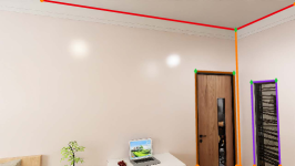
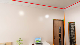
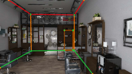
Semantic Room Wireframe Detection
from a Single View

Abstract

Reconstruction of indoor surfaces with limited texture information or with repeated textures, a situation common in walls and ceilings, may be difficult with a monocular Structure from Motion system. We propose a Semantic Room Wireframe Detection task to predict a Semantic Wireframe from a single perspective image. Such predictions may be used with shape priors to estimate the Room Layout and aid reconstruction. To train and test the proposed algorithm we create a new set of annotations from the simulated Structured3D dataset. We show qualitatively that the SRW-Net handles complex room geometries better than previous Room Layout Estimation algorithms while quantitatively out-performing the baseline in non-semantic Wireframe Detection.

Figure 1: The images on top show the desired results from Semantic Room Wireframe detection and below are the results from a Room Layout estimation algorithm [1]. Lines are added between all detected planes for comparison. The algorithm produces satisfying results on simple scenes (left) but is lacking on more complex scenes, e.g. to the right where the wide opening is erroneously classified as part of the wall.

I Introduction

Reconstruction of indoor spaces is useful for many applications, e.g. Virtual Reality, Real Estate sales and navigation for robots. Using consumer grade devices with a single camera (and possibly IMU) is preferred since this enables the application on a larger number of platforms. For this type of reconstruction one typically uses Structure from Motion (SfM) or Monocular Vision SLAM (Simultaneous Localization and Mapping). These rely on point features – points in the image with high saliency in terms of texture. This may be problematic in indoor spaces since most walls and ceilings are without salient textures.

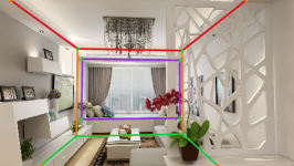
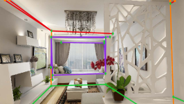
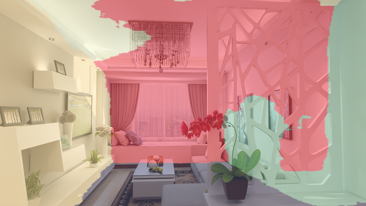
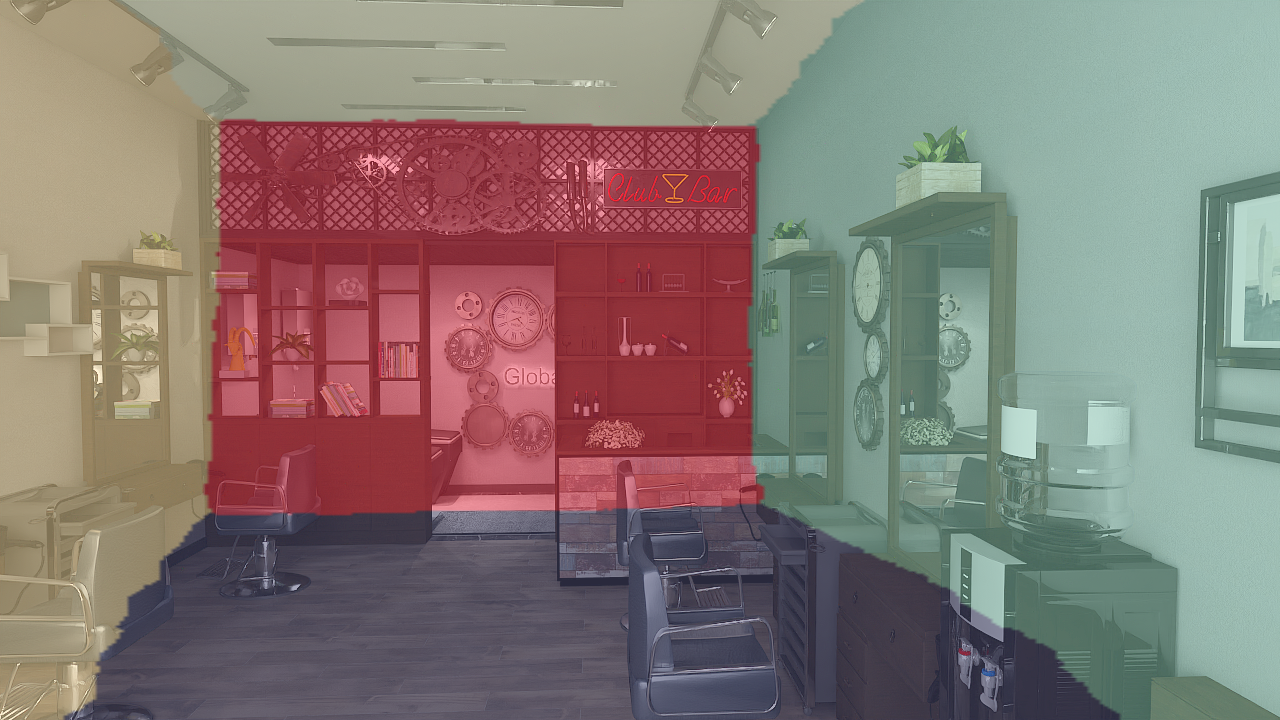
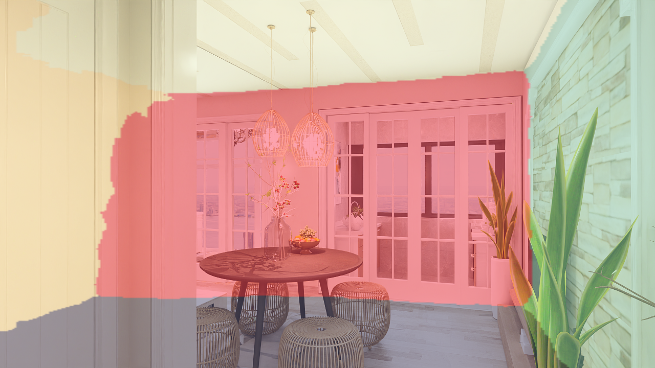
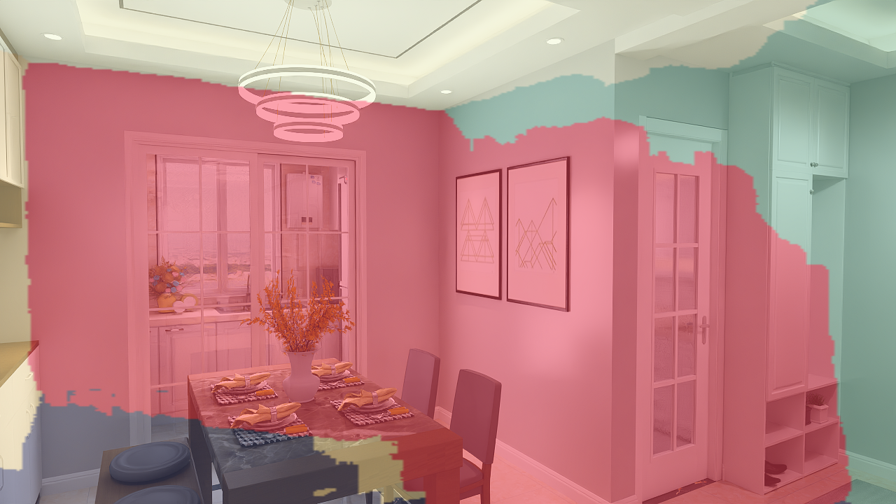
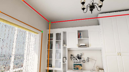
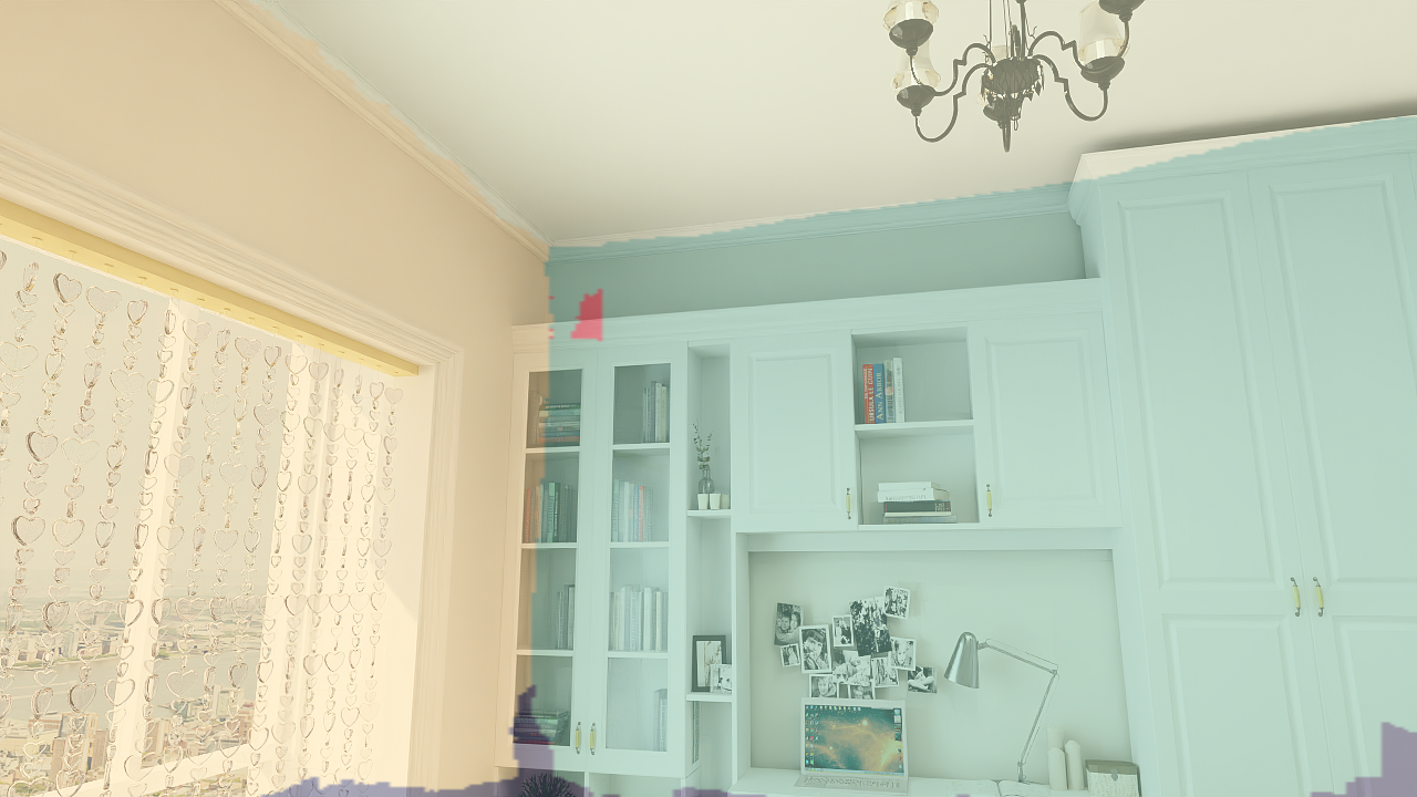
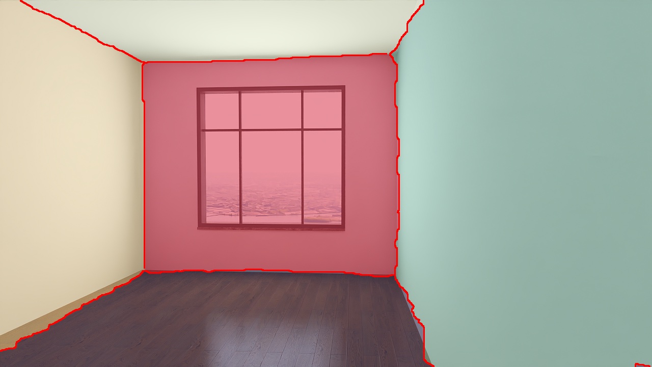
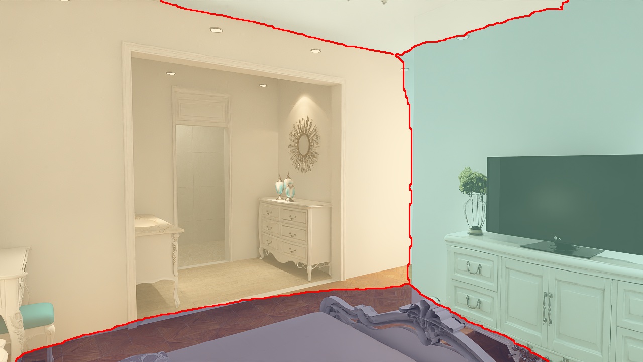
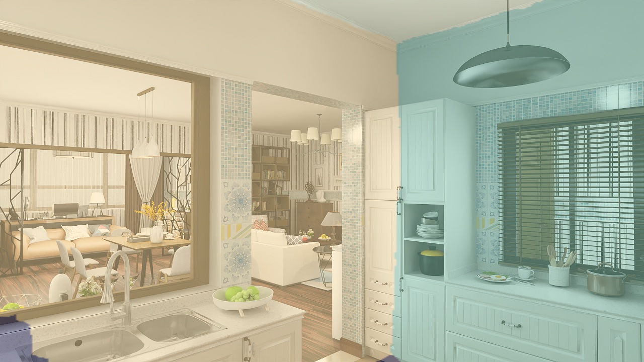
This has been the inspiration for research on Room Layout Estimation, which is the task of estimating the Room Geometry in terms of planar surfaces. Often strong priors about the relation between the surfaces are used and Room Geometries are assumed to be too simple, see Figure 1. Furthermore the multi-view case is often handled using Panorama, which is not always applicable.

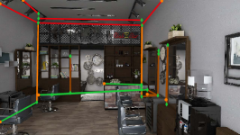
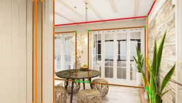
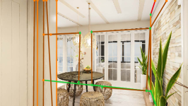
To relax the assumptions and handle multi-view scenarios we believe that the way forward is to develop several pipelines: semantic segmentation in the image, semantic segmentation in 3D, image object detection, corner detection and semantic line detection. These could then be used together – ideally in an end-to-end fashion. In this work our aim is to concentrate on one of these aspects and propose a Semantic Room Wireframe Detection task, where connected semantic line segments forming a wireframe, are to be detected. Since this is a detection task no strong assumptions are made and the detections can be used in a larger optimization framework to handle more complex Room Geometries captured from multiple views. Compared to previous methods we for example include labels for neighbouring rooms visible through open doors and label doors and windows in addition to the room structure.

We generate annotations, which consist of semantic line segments and semantic junctions from the synthetic Structured3D dataset. To perform the detection we adapt HAWP [2], which is a CNN (Convolutional Neural Network) developed for the Wireframe Detection task, and extend it with a Graph Convolutional Network (GCN) [3] module. We call the new network SRW-Net (Semantic Room Wireframe Network). We show qualitatively that the SRW-Net handles complex room geometries better than previous Room Layout Estimation algorithms while quantitatively out-performing HAWP [2] and L-CNN [4] for non-semantic Wireframe Detection. The contributions of this paper are:

• Proposal of the Semantic Room Wireframe detection task.

• New annotations for this task which we call Structured3D-SRW.

• Implementation and evaluation of a Neural Net for Semantic Room Wireframe detection, SRW-Net.

II Related Work

Room Layout Estimation was studied early by Hedau et al.[5] which used the Manhattan World assumption [6] as prior for the room shape. Early methods [7, 8, 9] used a pipeline which first extracted handcrafted features, then did vanishing point detection and lastly hypothesis generation and ranking. Recent approaches use CNNs, e.g. Mallya and Lazebnik [10] use structured edge detection forests, and a CNN to predict edge probability masks. Lin et al.[1] propose an end-to-end CNN with adaptive edge penalty and smoothness terms for pixelwise segmentation of the room image. RoomNet [11] directly predicts ordered keypoints in a room layout and DeepRoom3D [12] use an end-to-end CNN to predict a cuboid. Most recent methods [13, 14, 15, 16] use CNNs to predict edges and then optimize for the Room Layout using geometric priors. The datasets mostly used are LSUN [17] and Hedau [5].

Zhang et al.[18] advocated the use of Panorama images for increased performance in Room Layout Estimation. This has since been an inspiration for Panoramic Room Layout Estimation, which allows for better use of context and prior knowledge about camera orientation and calibration. Algorithms are typically based on CNNs [19, 20, 21] using different image representations and post-processing. For example CFL [22] predicts the 3D layout from a spherical image using edge and corner maps. Despite the promising results from these methods Room Layout Estimation from panorama does, indeed, limit the use of more conventional images. Common datasets for panorama are SUN360 [23], Stanford (2D-3D-S) [24] and Structured3D [25].

Recently, general Room Layout Estimation from a single perspective image, which does not assume cuboid shape, has been studied. [26] solves a discrete optimization problem over 3D polygons using both RGB and Depth information. [27] use plane detection to form a 3D model over a video sequence. [28] use a combination of plane, depth and vertical line detections to estimate a general Room Layout. Neither of these handle detections through open doorways. Data for this task is Structured3D [25] and ScanNet [29].

There is a vast literature on the use of lines for 3D understanding, even though SfM and SLAM are most often used in terms of points. For example understanding consistency constraints [30], exploiting such constraints for 3D understanding and SfM methods using only lines [31, 32, 33, 34, 35, 36, 37].

Detection of connected line segments has been studied as the task of Wireframe Estimation [38, 39, 40, 2]. However, these methods do not try to use semantic understanding of the lines and junctions and do not exploit such semantic understanding in terms of Room Layout Estimation. While recent works mostly form the Wireframe using junction proposals some works use line predictions directly. For example in [41], a combination of line predictions and graph networks are used. YorkUrban [42] and ShanghaiTech [43] are common datasets. Other approaches that predict semantic information for line segments [44] are focused around object detection rather than detection of indoor room structures.

III Semantic Room Wireframe Detection

We define a Semantic Room Wireframe Detection task. The prediction is done from a single perspective image and should result in a number of semantic lines in the image which – when connected by junctions – form a wireframe marking the intersections between the planes defining the room layout.

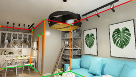
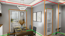
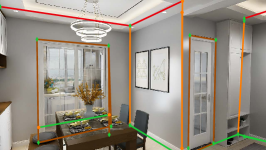
The task can be seen as a combination of Room Layout Estimation and Wireframe Detection. It is more flexible than Room Layout Estimation since no priors on the room structure are used but also contains more information than regular Wireframe Detection. The results can, e.g., be used to aid reconstructions, s.a. SfM and SLAM where salient textures are missing. It is also suitable for multi-view Room Layout Estimation, where it gives more flexibility for global optimization and better information in door openings. For an example of the desired output of a Semantic Room Wireframe Detector, see the top row of Figure 1.

IV Structured3D-SRW

Our annotations for this task, which we call Structured3D-SRW, are generated from Structured3D [25] which is a large-scale, photo-realistic simulated dataset with 3D structure annotations. It consists of 3500 scenes, with a total of 21’835 rooms and 196’515 frames. Structured3D contains 3D information about the room structure and is built up from junctions, lines and plane polygons. A junction is a point in $\mathbb{R}^{3}$ and a line is defined as the line segment formed by two junctions. A plane polygon is defined by a set of connected line segments and its parameters $\pi$ defining the normal vector and plane equation. These planes are labeled with semantic information, for example if the plane is a floor and part of a kitchen.

There are both panoramic and perspective images in the dataset. For each room, there are configurations both without furniture, with a little and with a lot of furniture. For each of the images, there is also a depth map and a semantic mask. The data is split so there are 3000 training, 250 validation and 250 testing scenes.

IV-A Data Analysis

Our annotations are generated by combining the 3D information, semantic masks and perspective RGB images with full furnishing. For the images with full furnishing there are 202 scenes missing from the training set, so that leaves us with 2’798 training scenes. While working with the data, we identified three main issues.

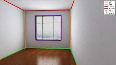
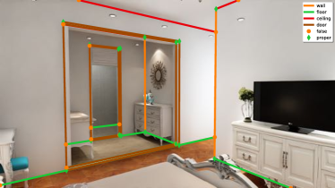
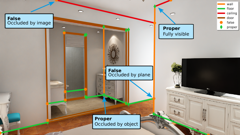
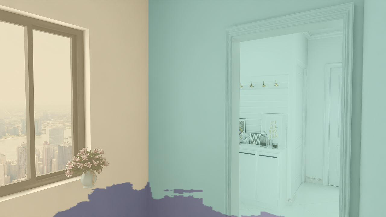
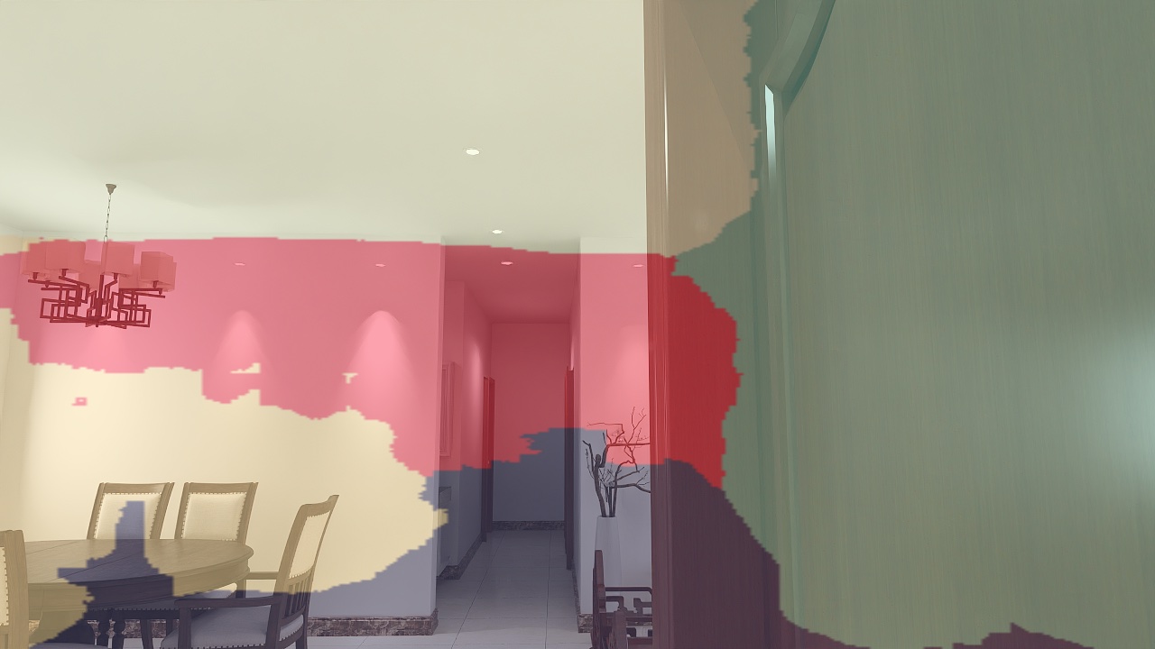
Firstly, there are a few planes to which only two junctions belong. However, only two junctions cannot uniquely define a plane. Secondly, it turns out that there are a number of planes for which the defining junctions do not lie in the plane. We calculated the Euclidean distance between all plane junctions and the plane according to supplied parameters and the result can be seen in Figure 2. We see that there are around $10^{3}$ planes with a maximum distance larger than 5mm. This is problematic since the assumption is that all surfaces are planar in this synthetic dataset. Thirdly, there is no information about whether the doors in Structured3D are open or closed. Since one of the strengths of our proposed method is that more complex structures can be captured, we want the method to identify open doors to create a wireframe also in the room behind them. One example of this can be seen in Figure 3, where the large opening in the left wall is annotated as a door. Knowing that it is open, we can train our method to detect the structure of the second room as well, as annotated in the image.

We have implemented the following measures to adjust for these three main issues:

(i) For the walls with only two junctions, we cannot form plane polygons to make occlusion checks. Because of this we simply discard the scenes containing such planes.

(ii) To verify that junctions lie in the plane, we chose to estimate new plane parameters from the junctions by solving the DLT problem

$$\min_{\|\pi\|^{2}=1}\|M\pi\|^{2},\;\text{for}\quad M =\begin{pmatrix}p_{1}&p_{2}&\ldots&p_{n}\end{pmatrix}^{T},$$ (1)

$$p_{i} =\begin{pmatrix}x_{i}&y_{i}&z_{i}&1\end{pmatrix}^{T},$$ (2)

where $p_{i}$ is a junction coordinate and $\pi$ are the four plane parameters s.t. a point $q$ is in the plane iff. $q^{T}\pi=0$. With these plane parameters we get lower maximum and median distances, compared to using the supplied parameters. Still, there are many planes that have large distances to their junctions. We therefore remove any scene with planes that have maximum error larger than 1mm. (i) and (ii) combined leaves us with 2’502, 218 and 205 scenes corresponding to 57’252, 5’684 and 5’085 images for training, validation and testing, respectively.

(iii) We do the following to determine whether doors are open or closed: For each door polygon $D_{i,j}$ belonging to wall plane $\pi_{i}$ we take a set of 100 uniformly distributed sample points $\hat{D}_{i,j}=\{p_{k}\in D_{i,j}\}$. For each sample set $\hat{D}_{i,j}$ and each perspective image $\hat{I}_{l}$ for a scene, we find the sample points

$$\hat{D}^{l}_{i,j}=\left\{(x_{k},y_{k},1)^{T}\sim P_{l}p_{k}\;\middle|\;(x_{k},y_{k})\in\hat{I}_{l}\right\},$$ (3)

in pixel coordinates using the camera matrix $P_{l}=K_{l}[R_{l}\;t_{l}]$, where $K_{l}$ are intrinsic parameters, $R_{l}$ rotation matrix and $t_{l}$ translation vector. We then compute a door closed ratio

$$c_{i,j}=\frac{\sum_{l}\sum_{k}\alpha_{lk}}{\sum_{l}\sum_{k}1},\qquad\alpha_{lk}=\begin{cases}1,\,\text{if}\;\hat{I}_{l}[y_{k},x_{k}]=\textit{door}{},\\ 0,\,\text{otherwise},\end{cases}$$ (4)

and say that the door $\hat{D}_{i,j}$ is closed if $c_{i,j}>0.3$.

Figure 2: Histograms for the maximum, median and minimum distance from each plane to its junctions using the supplied plane equation. Note that the plane parameters are not optimized to minimize distance to all junctions.

IV-B Semantic Information

In Structured3D each plane is annotated with a type and a semantic class. By combining the information in these two fields we mark each plane as either wall, floor, ceiling, door or window.

We choose to have one label per line and define each line label as the combination of the two planes it belongs to. If we look at the last column of Table I we see that there are seven occurring classes, where door and window planes yield two different line labels each. Since most of the door-door and window-window lines will be concealed behind doors and window glass we choose to merge these with door-wall and window-wall, respectively. We then get the mapping in Table I, which consists of the same five labels as for the planes, namely wall, floor, ceiling, door and window.

Furthermore, we also label the junctions. The dataset consists of two different kinds of junctions. There are junctions corresponding to a 3D junction where three planes meet; these we call proper and they should be detected even when occluded by furniture. There are also junctions which occur either due to the camera having limited field of view, or due to occlusion from other planes. These we call false. See Figure 3 for an example.

TABLE I: Mapping of line labels from plane labels.

Line label	Plane labels	Occurrence [%]
door	door-wall	20.4
wall	wall-wall	15.5
ceiling	ceiling-wall	15.5
floor	floor-wall	15.5
door	door-door	11.6
window	window-wall	11.0
window	window-window	10.4

Figure 3: Example cases for junction labels proper and false .

V SRW-Net

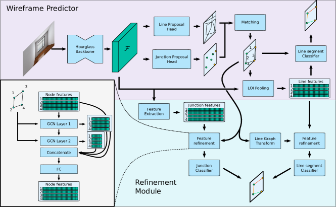
For the CNN architecture we chose to base it on HAWP (Holistically-Attracted Wireframe Parsing), presented in Xue et al.[2]. Since our data contains semantic labels for both lines and junctions, but fewer lines per image, we had to make some adjustments to the architecture and parameters. In addition to the changes we introduce a GCN module, trained separately, to refine the features using neighbours in the wireframe. See Figure 4 for an overview of the architecture.

Figure 4: An overview of the SRW-Net architecture.

V-A Backbone

Before fed into the network, the image is resized to $H\times W$ pixels, where $H=W=512$. It is then passed through a backbone Hourglass Network [45] which generates a latent feature space $\mathcal{F}$ of size $N\times\hat{H}\times\hat{W}$, where $\hat{H}=\hat{W}=128$ and $N=128$ is the number of channels. These features are then used by the different network heads.

V-B Junction Proposals

The junction proposal head predicts from $\mathcal{F}$ a junction label matrix $\mathcal{J}$ of size $3\times\hat{H}\times\hat{W}$ with one-hot encoding for labels invalid, false, proper. It also predicts an offset matrix $\mathcal{O}$ of size $2\times\hat{H}\times\hat{W}$. They are computed using a $1\times 1$ convolutional layer and then sigmoid for $\mathcal{O}$ and softmax for $\mathcal{J}$. This is different from HAWP since they did not have labels for junctions and used sigmoid for $\mathcal{J}$. We then form $\mathcal{J}_{v}=1-\mathcal{J}[\textit{invalid}{}]$. After a $3\times 3$ NMS (Non-Maximum Suppression) to $\mathcal{J}_{v}$ the top $K$ bins $\mathcal{J}_{K}=\{(x_{k},y_{k}),k=1...K\}$ are selected ($K=80$) and the offset map is used to compute the final position of the junctions $\mathcal{J}_{f}=\{(x_{k},y_{k})+\mathcal{O}(x_{k},y_{k})\cdot w,k=1...K\}$ where $w$ is a rescaling factor. Like HAWP we use cross entropy loss to form $\mathbb{L}(\mathcal{J},\hat{\mathcal{J}})$ and L1 loss for $\mathbb{L}(\mathcal{O},\hat{\mathcal{O}})$. But we weight invalid as 1:250 in $\mathbb{L}(\mathcal{J},\hat{\mathcal{J}})$ to account for bias and improve recall. The final loss function is $\mathbb{L}_{j}=\lambda_{msk}\cdot\mathbb{L}(\mathcal{J},\hat{\mathcal{J}})+\lambda_{off}\cdot\mathcal{J}_{v}\odot\mathbb{L}(\mathcal{O},\hat{\mathcal{O}})$, where $\odot$ is elementwise multiplication, $\lambda_{msk}$ and $\lambda_{off}$ are design parameters.

V-C Line Segment Proposal

The line segment proposal head is the same as for HAWP and is a modification of AFM [39] which uses a parametrization of line segments using four parameters. It is, however, not unique and each parametrization may yield up to three line segments. The proposal head takes $\mathcal{F}$ and predicts a $4\times\hat{H}\times\hat{W}$ matrix, where the first dimension is the 4D AFM parametrization, which is then converted to the endpoint line segment representation. The loss function is the same as for HAWP and we denote it $\mathbb{L}_{LS}$.

V-D Line Segment and Junction Proposal Matching

Now we have line segment proposals and junction proposals. Each line segment’s endpoints are matched to their closest junction. If the Euclidean distance between each endpoint and matched junction is below $\tau=10$, we form a line segment between these two junctions. We denote the set of matched line segments $\mathcal{L}_{m}$.

V-E Matched line segment classification

Each matched line segment $l\in\mathcal{L}_{m}$ will be classified as either invalid, wall, floor, ceiling, window or door. Following the implementation of HAWP we use the LoIPool operation [4] from L-CNN. First $s=32$ uniformly spaced points along the line are sampled from $\mathcal{F}$. All features are then reduced, concatenated and given to the 2-layer fully connected classifier ending with the softmax operation and cross entropy loss $\mathbb{L}_{cls}$. This is trained end to end and the final loss is $\mathbb{L}=\mathbb{L}_{junc}+\mathbb{L}_{LS}+\mathbb{L}_{cls}$. During training we balance negative and positive examples while also providing hard negative examples from the ground truth data, see HAWP [2] for details. We reduced the number of sampled lines to 100 negative and 100 positive.

V-F Wireframe Refinement - Graph Convolutional Network

This GCN module uses the graph structure to augment the line and junction features with encoded features from the neighbouring lines and junctions prior to classification. The module is trained separately from the larger network and takes lines with invalid score less than $0.95$ as input. We form two graphs, the junction graph is simply the estimated wireframe where junction features are nodes and lines define edges. The line segment graph is created by taking the Line Graph [46] of the junction graph, s.t. the line segment features now are nodes. The architecture of the GCN layers are encoder-based with skip-connections to a fully connected classifier layer, see Figure 4. We use 4 GCN layers for junction and line head respectively. To achieve good results we sample positive and negative examples as 5:1 for the loss function. The loss and classifier architecture are the same as previously.

VI Evaluation

sAP (structural average precision) [4] is the area under the precision and recall curve for a set of scored detected line segments. Let $\hat{L}=\begin{pmatrix}\hat{p_{1}}&\hat{p_{2}}\end{pmatrix}\in\mathcal{L}_{g}$ be any line segment in the set of true line segments. A detected line segment $L=\begin{pmatrix}p_{1}&p_{2}\end{pmatrix}$ is a true positive if

$$\min_{\hat{L}\in\mathcal{L}_{g}}\delta(L,\hat{L})=\|p_{1}-\hat{p}_{1}\|^{2}_{2}+\|p_{2}-\hat{p}_{2}\|^{2}_{2}\leq\beta,$$ (5)

where $\beta$ is a design parameter. We also require that only one detection is matched to each true line segment. Any extra predictions are marked as false positives. In our experiments we evaluate the metric at $\beta=5,10,15$ at $128\times 128$ resolution and denote the metrics $\text{sAP}^{5}$, $\text{sAP}^{10}$ and $\text{sAP}^{15}$ respectively. We calculate sAP for each separate label and then take the mean to form msAP. We also calculate $\text{sAP}^{m}=\sum_{\beta}\text{sAP}^{\beta}/3$ for each label and take its mean across labels as $\text{msAP}^{m}$.

NMS (Non Maximum Suppression) is also performed on line segments to improve performance. We use the same distance $\delta$ as in Equation (5) and say that if a line segment $L$ has a neighbour $\hat{L}$ s.t. $\delta(L,\hat{L})<\gamma^{2}$ with the same predicted label and higher score, $L$ is removed. We use $\gamma=3$.

jAP (junction AP), is analogous to sAP. Instead of the criteria in Equation (5) we take the Euclidean distance between the junction and the closest ground truth junction of the same label. The thresholds are $0.5$, $1.0$ and $2.0$ and $\text{mjAP}^{m}$, $\text{jAP}^{m}$ follows as before.

VII Experiments

All experiments were done using pre-trained weights from HAWP as initialization for applicable layers, as we noticed this produced better results than training from scratch. Models were trained for 40 epochs with learning rate $4\cdot 10^{-4}$, weight decay $10^{-4}$ and batch size $11$ on a Nvidia Titan V. The learning rate was reduced to $4\cdot 10^{-5}$ at epoch 25. For the GCN refinement module we trained for 10 epochs with learning rate $1.2\cdot 10^{-3}$, weight decay $10^{-4}$ and batch size $60$. The learning rate was reduced to $1.2\cdot 10^{-4}$ at epoch 5.

VII-A Model evaluation

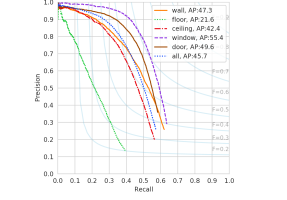
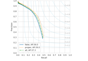
We evaluate the proposed model on the test set. See Table II for AP numbers and Figure 5 for the PR (precision recall) curve for threshold 10. We see that floor is by far the most difficult line type to detect correctly. Since there is no method available for direct comparison we trained HAWP [2] and L-CNN [4] on Structured3D-SRW using their code and training methods. All models are initiated with the pre-trained weights provided by the code releases. Since these algorithms output a non-semantic wireframe we generate a wireframe prediction from our method by calculating the score as $(1-\textit{invalid}{})$ for junctions and lines. In Table III we see that our method out-performs both HAWP and L-CNN in line segment detection (sAP). HAWP performs better in the junction metric jAP.

TABLE II: AP Scores for the final model.

Type	$\text{sAP}^{5}$	$\text{sAP}^{10}$	$\text{sAP}^{15}$	$\text{sAP}^{m}$
ceiling	35.5	42.4	46.5	41.5
door	44.7	49.6	52	48.8
floor	15.5	21.6	24.6	20.6
wall	39.8	47.3	51.2	46.1
window	49.5	55.4	58.2	54.4
mAP	37	43.3	46.5	42.3
Type	$\text{jAP}^{0.5}$	$\text{jAP}^{1}$	$\text{jAP}^{2}$	$\text{jAP}^{m}$
false	17.8	36	43.7	32.5
proper	21.9	39	46.8	35.9
mAP	19.9	37.5	45.3	34.2

TABLE III: Comparision of the (1-invalid) score against HAWP and L-CNN.

Arch.	$\text{sAP}^{m}$	$\text{jAP}^{m}$
LCNN	31.8	34.9
HAWP	46.0	37.0
SRW	46.6	36.2

Figure 5: Left: $\text{sAP}^{10}$ PR curve for line segments. Right: $\text{jAP}^{1}$ PR curve for junctions. Note that floor is the most difficult line label to predict. While all junction labels are equally difficult.

Figure 6: Results from the comparison with Room Layout Estimation. On top: the original images with Semantic Wireframe annotations. In the middle: the results from our method. In the bottom: Room Layout results from [1].

VII-B Ablation study

In Table IV we show results on how the class weights for the junction loss $\mathbb{L}(\mathcal{J},\hat{\mathcal{J}})$, the GCN refinement module and line NMS affects the classification for the validation set. Although equal weights for $\mathbb{L}(\mathcal{J},\hat{\mathcal{J}})$ outperforms a weighted loss in $\text{sAP}^{m}$ the GCN refinement module benefits from the improved $\text{jAP}^{m}$ and recall. Therefore the weighted loss with GCN refinement module and line NMS has the best performance.

TABLE IV: Ablation study on validation set.

GCN	NMS	$\mathbb{L}(\mathcal{J},\hat{\mathcal{J}})$	$\text{sAP}^{m}$	$\text{jAP}^{m}$
		equal	44.6	26.4
		weighted	31.6	37.4
✓		equal	45.0	39.0
✓		weighted	45.3	37.9
✓	✓	equal	45.8	37.9
✓	✓	weighted	46.7	37.9

VII-C Room Layout vs Semantic Room Wireframe

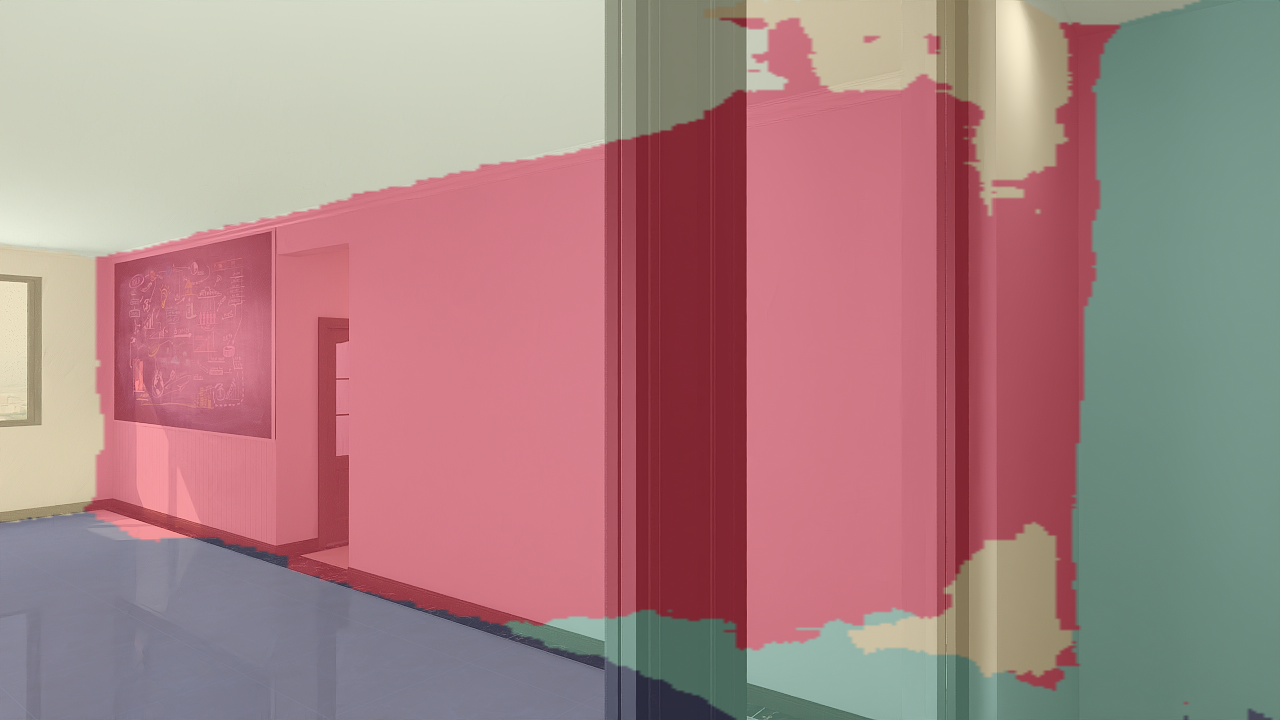
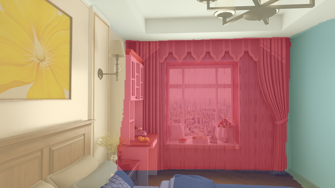
We make a qualitative comparison in Figure 6 with the method of Lin et al.[1] from the Room Layout Estimation task to illustrate the benefits of this data. For our method we use all lines with score higher than 0.9. Since the methods are trained on different data we cannot compare performance, but we see that the representation for the Room Layout Estimation task is not sufficient for these complex scenes.

VIII Conclusions

We have introduced the task of Semantic Room Wireframe detection and generated annotations from Structured3D. This dataset challenges algorithms to detect complex Room Geometries from single view perspective images. We show that a CNN for Wireframe estimation can be adapted to this task and handles complex Room Geometries better than a reference method for Room Layout Estimation. We also show how the graph structure can be used with a GCN refinement module to out-perform the baseline even in non-semantic wireframe detection.

A-i Introduction

This is supplementary material for our paper "Semantic Room Wireframe Detection from a Single View". It further describes the data generation process and provides more images for qualitative evaluation.

A-ii Structured3D-SRW Data Generation

This section gives a brief explanation on how our dataset Structured3D-SRW, described in Section IV of the paper, is generated. For further details we refer to the code.

First we define for a point $r=\begin{pmatrix}x_{1}&x_{2}&\ldots&x_{n}\end{pmatrix}\in\mathbb{R}^{n}$ and its corresponding point $p=\begin{pmatrix}y_{1}&y_{2}&\ldots&y_{n+1}\end{pmatrix}\in\mathbb{P}^{n}$ in homogeneous coordinates the mapping function

$$\mathbb{P}^{n}\rightarrow\mathbb{R}^{n}:\phi(p)=\begin{pmatrix}\frac{y_{1}}{y_{n+1}}&\frac{y_{2}}{y_{n+1}}&\ldots&\frac{y_{n}}{y_{n+1}}\end{pmatrix}.$$ (6)

The task is to generate a set of junctions $J_{i}$ connected by edges $E_{i}$ for each image $I_{i}$. To simplify we will consider a single line segment $\hat{l}=\begin{pmatrix}\hat{p_{1}}&\hat{p_{2}}\end{pmatrix}$ with endpoints $\hat{p}_{1},\hat{p}_{2}\in\mathbb{P}^{3}$ s.t $\phi(\hat{p}_{1}),\phi(\hat{p}_{2})\in\mathbb{R}^{3}$ are in the scene coordinate system. as well as the scene’s defining set of planes, which have polygons $W=\{w_{k},k=1,...,N\}$ and plane parameters

$$\hat{\Pi}=\left\{\hat{\pi}_{k}=\begin{pmatrix}\hat{n}_{k}\\ \hat{d}\end{pmatrix}\;\middle|\;\|\hat{n}_{k}\|=1,\phi(p)\in w_{k}\Rightarrow p^{T}\hat{\pi}_{k}=0\right\},$$ (7)

where $\hat{n}_{k}\in\mathbb{R}^{3}$ is the normal vector.

For now we assume that the line segment is in front of the camera and inside the image. We start by transforming the planes and line segment to the camera centered coordinate system

$$L=\begin{pmatrix}p_{1}&p_{2}\end{pmatrix}=T_{i}\hat{L},\quad\\ \Pi=\left\{\pi_{k}=T^{-1}\hat{\pi}_{k}\;\middle|\;\hat{\pi}\in\hat{\Pi}\right\},\;\text{where}\;T_{i}=\begin{pmatrix}R_{i}&t_{i}\\ 0&1\end{pmatrix}.$$ (8)

For each plane $\pi_{k}$ we find where on the viewing ray for line segment endpoint $p_{j}$ we have the plane. So if

$$a_{j}=-\frac{d_{k}}{\phi(p_{j})^{T}n_{k}}$$ (9)

we know that $0<a_{j}<1$ if the point is occluded. Now we have four cases

• $a_{1},a_{2}\geq 1\Rightarrow$ The entire line segment is in front of plane, we are done.

• $a_{1},a_{2}\leq 0\Rightarrow$ The plane is behind the camera, we are done.

• $a_{1},a_{2}<1\Rightarrow$ The line segment is behind the plane, $L_{b}=L$.

• For all other cases a part of the line segment is in front of the plane. We form the line segment $L_{b}$ which is behind the plane and $L_{f}$ which is in front.

Now we can project $L_{b}$ onto the plane $\pi_{k}$ and take the 2D geometric difference to get a set of line segments

$$\hat{L}_{w}=\left(\begin{pmatrix}a_{1}\\ a_{2}\end{pmatrix}\odot L_{b}\right)-w_{k},$$ (10)

where $\odot$ is elementwise multiplication. These are in the plane $\pi_{k}$ so we so we find the corresponding line segments on $L$ and denote them $L_{w}$. We then merge $L_{f}$ with $L_{w}$ and get the visible set of line segments which we transform back to the camera coordinate system and apply $K_{i}$ to get the pixel coordinates. An overview of the algorithm is given in Algorithm 1. Please refer to the implementation code for details.

Data: Parameters of scene planes: $\hat{\Pi}$, Semantic images: $\hat{\textbf{I}}$, RGB images: I, All plane junctions: J, All scene lines: $\hat{\textbf{L}}$,

Result: Set of visible line segments $\textbf{L}^{i}_{V}$ for each image $i$

$W:=$ makePolygons($\hat{\textbf{I}},\hat{\Pi},\textbf{J}$);

for $I_{i}\in\textbf{I}$ do

       $\Pi:=T^{-1}_{i}\hat{P_{i}}$;

       $\textbf{L}:=T_{i}\hat{\textbf{L}}$;

       for $L\in\textbf{L}$ do

             $L:=$cutInFrontAndInImage($L$);

             if $L=\emptyset$ then

                   continue ;

                  

             end if

            $\textbf{L}^{i}_{V}=\{L\}$ ;

             for $w_{k}\in W,\pi_{k}\in\Pi$ do

                   $L_{t}:=\emptyset$;

                   for $L\in L^{i}_{V}$ do

                         $L_{f},L_{b}:=$ behindPlane($\pi_{k},L$);

                         $\textbf{L}_{p}:=$ inPolygon($L_{b}$);

                         $L_{t}:=L_{t}\cup$ appendLine($\textbf{L}_{p},L_{f}$);

                        

                   end for

                  $\textbf{L}^{i}_{V}:=L_{t}$;

                  

             end for

            

       end for

      

end for

Algorithm 1 An overview of how the algorithm to annotate one scene works. For details and special cases please refer to the implementation code.

A-iii Plane estimation

In Section IV-A we estimate new plane parameters that fit optimally with the plane junction. See Figure 7 for the histograms of distances from plane to junctions.

Figure 7: Histograms for the maximum, median and minimum distance from each plane to its junctions using the estimated plane equation.

A-iv Additional Images for Qualitative Comparison

Here is and extension to Section VII-C of the paper, where we compared SRW-Net a Room Layout estimation algorithm [1]. For additional images from Structured3D-SRW, see Figure 8.

Figure 8: Results from the comparison with room layout estimation. On the left: images with ground truth semantic wireframe annotations. In the middle: the results from our method. To the right: room layout results from [1].

References

- [1] H. J. Lin, S.-W. Huang, S.-H. Lai, and C.-K. Chiang, “Indoor scene layout estimation from a single image,” in 2018 24th International Conference on Pattern Recognition (ICPR), 2018.
- [2] N. Xue, T. Wu, S. Bai, F.-D. Wang, G.-S. Xia, L. Zhang, and P. H. Torr, “Holistically-attracted wireframe parsing,” in IEEE Conference on Computer Vision and Pattern Recognition (CVPR), 2020.
- [3] T. N. Kipf and M. Welling, “Semi-supervised classification with graph convolutional networks,” in 5th International Conference on Learning Representations, ICLR 2017, Toulon, France, April 24-26, 2017, Conference Track Proceedings, 2017.
- [4] Y. Zhou, H. Qi, and Y. Ma, “End-to-end wireframe parsing,” in ICCV 2019, 2019.
- [5] V. Hedau, D. Hoiem, and D. Forsyth, “Recovering the spatial layout of cluttered rooms,” in 2009 IEEE 12th international conference on computer vision. IEEE, 2009, pp. 1849–1856.
- [6] J. M. Coughlan and A. L. Yuille, “Manhattan world: compass direction from a single image by bayesian inference,” in Proceedings of the Seventh IEEE International Conference on Computer Vision, vol. 2, 1999, pp. 941–947 vol.2.
- [7] A. Schwing, T. Hazan, M. Pollefeys, and R. Urtasun, “Efficient structured prediction for 3d indoor scene understanding,” in 2012 IEEE Conference on Computer Vision and Pattern Recognition, CVPR 2012, ser. Proceedings of the IEEE Computer Society Conference on Computer Vision and Pattern Recognition, 2012, pp. 2815–2822.
- [8] L. Del Pero, J. Bowdish, D. Fried, B. Kermgard, E. Hartley, and K. Barnard, “Bayesian geometric modeling of indoor scenes,” in 2012 IEEE Conference on Computer Vision and Pattern Recognition, CVPR 2012, ser. Proceedings of the IEEE Computer Society Conference on Computer Vision and Pattern Recognition, Oct. 2012, pp. 2719–2726, 2012 IEEE Conference on Computer Vision and Pattern Recognition, CVPR 2012 ; Conference date: 16-06-2012 Through 21-06-2012.
- [9] W. Zhang, W. Zhang, and J. Gu, “Edge-semantic learning strategy for layout estimation in indoor environment,” CoRR, vol. abs/1901.00621, 2019. [Online]. Available: http://arxiv.org/abs/1901.00621
- [10] A. Mallya and S. Lazebnik, “Learning informative edge maps for indoor scene layout prediction,” in 2015 International Conference on Computer Vision, ICCV 2015, ser. Proceedings of the IEEE International Conference on Computer Vision. United States: Institute of Electrical and Electronics Engineers Inc., Feb. 2015, pp. 936–944, 15th IEEE International Conference on Computer Vision, ICCV 2015 ; Conference date: 11-12-2015 Through 18-12-2015.
- [11] C.-Y. Lee, V. Badrinarayanan, T. Malisiewicz, and A. Rabinovich, “Roomnet: End-to-end room layout estimation,” 2017.
- [12] H. J. Lin and S.-H. Lai, “Deeproom: 3d room layout and pose estimation from a single image,” in Pattern Recognition, S. Palaiahnakote, G. Sanniti di Baja, L. Wang, and W. Q. Yan, Eds. Cham: Springer International Publishing, 2020, pp. 719–733.
- [13] Y. Ren, S. Li, C. Chen, and C.-C. J. Kuo, “A coarse-to-fine indoor layout estimation (cfile) method,” in Computer Vision – ACCV 2016, S.-H. Lai, V. Lepetit, K. Nishino, and Y. Sato, Eds. Cham: Springer International Publishing, 2017, pp. 36–51.
- [14] H. Zhao, M. Lu, A. Yao, Y. Guo, Y. Chen, and L. Zhang, “Physics inspired optimization on semantic transfer features: An alternative method for room layout estimation,” 2017.
- [15] C. Yan, B. Shao, H. Zhao, R. Ning, Y. Zhang, and F. Xu, “3d room layout estimation from a single rgb image,” IEEE Transactions on Multimedia, vol. 22, no. 11, pp. 3014–3024, 2020.
- [16] I. Kruzhilov, M. Romanov, D. Babichev, and A. Konushin, “Double refinement network for room layout estimation,” in Pattern Recognition. Cham: Springer International Publishing, 2020, pp. 557–568.
- [17] F. Yu, A. Seff, Y. Zhang, S. Song, T. Funkhouser, and J. Xiao, “Lsun: Construction of a large-scale image dataset using deep learning with humans in the loop,” 2016.
- [18] Y. Zhang, S. Song, P. Tan, and J. Xiao, “Panocontext: A whole-room 3d context model for panoramic scene understanding,” in Computer Vision – ECCV 2014, D. Fleet, T. Pajdla, B. Schiele, and T. Tuytelaars, Eds. Cham: Springer International Publishing, 2014, pp. 668–686.
- [19] C. Zou, A. Colburn, Q. Shan, and D. Hoiem, “Layoutnet: Reconstructing the 3d room layout from a single rgb image,” in Proceedings of the IEEE Conference on Computer Vision and Pattern Recognition, 2018, pp. 2051–2059.
- [20] S.-T. Yang, F.-E. Wang, C.-H. Peng, P. Wonka, M. Sun, and H.-K. Chu, “Dula-net: A dual-projection network for estimating room layouts from a single rgb panorama,” in Proceedings of the IEEE/CVF Conference on Computer Vision and Pattern Recognition, 2019, pp. 3363–3372.
- [21] C. Sun, C.-W. Hsiao, M. Sun, and H.-T. Chen, “Horizonnet: Learning room layout with 1d representation and pano stretch data augmentation,” in Proceedings of the IEEE/CVF Conference on Computer Vision and Pattern Recognition, 2019, pp. 1047–1056.
- [22] C. Fernandez-Labrador, J. M. Facil, A. Perez-Yus, C. Demonceaux, J. Civera, and J. J. Guerrero, “Corners for layout: End-to-end layout recovery from 360 images,” IEEE Robotics and Automation Letters, vol. 5, no. 2, pp. 1255–1262, 2020.
- [23] J. Xiao, K. A. Ehinger, A. Oliva, and A. Torralba, “Recognizing scene viewpoint using panoramic place representation,” in IEEE Conference on Computer Vision and Pattern Recognition (CVPR), Jun. 2012.
- [24] I. Armeni, S. Sax, A. R. Zamir, and S. Savarese, “Joint 2d-3d-semantic data for indoor scene understanding,” 2017.
- [25] J. Zheng, J. Zhang, J. Li, R. Tang, S. Gao, and Z. Zhou, “Structured3d: A large photo-realistic dataset for structured 3d modeling,” in Proceedings of The European Conference on Computer Vision (ECCV), 2020.
- [26] S. Stekovic, S. Hampali, M. Rad, S. D. Sarkar, F. Fraundorfer, and V. Lepetit, “General 3d room layout from a single view by render-and-compare,” in Computer Vision – ECCV 2020. Cham: Springer International Publishing, 2020, pp. 187–203.
- [27] H. Howard-Jenkins, S. Li, and V. A. Prisacariu, “Thinking outside the box: Generation of unconstrained 3d room layouts,” in ACCV, 2018.
- [28] C. Yang, J. Zheng, X. Dai, R. Tang, Y. Ma, and X. Yuan, “Learning to reconstruct 3d non-cuboid room layout from a single rgb image,” in WACV, 2022.
- [29] A. Dai, A. X. Chang, M. Savva, M. Halber, T. Funkhouser, and M. Nießner, “Scannet: Richly-annotated 3d reconstructions of indoor scenes,” in Proc. Computer Vision and Pattern Recognition (CVPR), IEEE, 2017.
- [30] A. Heyden, “Consistency and correction of line-drawings, obtained by projections of piecewise planar objects,” in European Conference on Computer Vision. Springer, 1994, pp. 411–419.
- [31] F. Kahl and A. Heyden, “Structure and motion from points, lines and conics with affine cameras,” in European Conference on Computer Vision. Springer, 1998, pp. 327–341.
- [32] K. Åström, A. Heyden, F. Kahl, and M. Oskarsson, “Structure and motion from lines under affine projections,” in Proceedings of the Seventh IEEE International Conference on Computer Vision, vol. 1. IEEE, 1999, pp. 285–292.
- [33] M. Oskarsson, A. Zisserman, and K. Åström, “Minimal projective reconstruction for combinations of points and lines in three views,” Image and Vision Computing, vol. 22, no. 10, pp. 777–785, 2004.
- [34] A. Bartoli and P. Sturm, “Structure-from-motion using lines: Representation, triangulation, and bundle adjustment,” Computer vision and image understanding, vol. 100, no. 3, pp. 416–441, 2005.
- [35] V. Larsson, K. Åström, and M. Oskarsson, “Efficient solvers for minimal problems by syzygy-based reduction,” in Proceedings of the IEEE Conference on Computer Vision and Pattern Recognition, 2017, pp. 820–829.
- [36] B. Micusik and H. Wildenauer, “Structure from motion with line segments under relaxed endpoint constraints,” International Journal of Computer Vision, vol. 124, no. 1, pp. 65–79, 2017.
- [37] T. Lemaire and S. Lacroix, “Monocular-vision based slam using line segments,” in Proceedings 2007 IEEE International Conference on Robotics and Automation. IEEE, 2007, pp. 2791–2796.
- [38] G.-S. Xia, J. Delon, and Y. Gousseau, “Accurate junction detection and characterization in natural images,” International journal of computer vision, vol. 106, no. 1, pp. 31–56, 2014.
- [39] N. Xue, S. Bai, F. Wang, G.-S. Xia, T. Wu, and L. Zhang, “Learning attraction field representation for robust line segment detection,” in Proceedings of the IEEE/CVF Conference on Computer Vision and Pattern Recognition, 2019, pp. 1595–1603.
- [40] N. Xue, S. Bai, F.-D. Wang, G.-S. Xia, T. Wu, L. Zhang, and P. H. Torr, “Learning regional attraction for line segment detection,” IEEE transactions on pattern analysis and machine intelligence, 2019.
- [41] Q. Meng, J. Zhang, Q. Hu, X. He, and J. Yu, LGNN: A Context-Aware Line Segment Detector. New York, NY, USA: Association for Computing Machinery, 2020, p. 4364–4372. [Online]. Available: https://doi.org/10.1145/3394171.3413784
- [42] N.-G. Cho, A. Yuille, and S.-W. Lee, “A novel linelet-based representation for line segment detection,” IEEE Transactions on Pattern Analysis and Machine Intelligence, vol. 40, no. 5, pp. 1195–1208, 2018.
- [43] K. Huang, Y. Wang, Z. Zhou, T. Ding, S. Gao, and Y. Ma, “Learning to parse wireframes in images of man-made environments,” in Proceedings of the IEEE Conference on Computer Vision and Pattern Recognition (CVPR), June 2018.
- [44] Y. Sun, X. Han, K. Sun, B. Li, Y. Chen, and M. Li, “Sem-lsd: A learning-based semantic line segment detector,” 2019.
- [45] A. Newell, K. Yang, and J. Deng, “Stacked hourglass networks for human pose estimation,” in Computer Vision - 14th European Conference, ECCV 2016, Proceedings, ser. Lecture Notes in Computer Science (including subseries Lecture Notes in Artificial Intelligence and Lecture Notes in Bioinformatics). Germany: Springer Verlag, 2016, pp. 483–499.
- [46] L. W. Beineke, “Characterizations of derived graphs,” Journal of Combinatorial Theory, vol. 9, no. 2, pp. 129–135, 1970. [Online]. Available: https://www.sciencedirect.com/science/article/pii/S0021980070800199