One- and two-dimensional solitons in spin-orbit-coupled Bose-Einstein condensates with fractional kinetic energy

Abstract

We address effects of spin-orbit coupling (SOC), phenomenologically added to a two-component Bose-Einstein condensate composed of particles moving by Lévy flights, in one- and two-dimensional (1D) and (2D) settings. The corresponding system of coupled Gross-Pitaevskii equations includes fractional kinetic-energy operators, characterized by the Lévy index, $\alpha<2$ (the normal kinetic energy corresponds to $\alpha=2$). The SOC terms, with strength $\lambda$, produce strong effects in the 2D case: they create families of stable solitons of the semi-vortex (SV) and mixed-mode (MM) types in the interval of $1<\alpha<2$, where the supercritical collapse does not admit the existence of stable solitons in the absence of the SOC. At $\lambda\rightarrow 0$, amplitudes of these solitons vanish $\sim\lambda^{1/(\alpha-1)}$.

I Introduction

The concept of derivatives of fractional orders was proposed in 1823 by Niels Henrik Abel Abel . In physics, the implementation of the fractionality was proposed by N. Laskin Laskin , who had introduced a linear fractional differential operator (actually, it is defined by an integral expression, see Eq. (2) below) which replaces the usual quantum-mechanical kinetic energy. The result is the fractional Schrödinger equation (FSE) for wave function $\psi(x,t)$, with the Lévy index $\alpha$, time $t$, spatial coordinate $x$, and potential $U(x)$. The normalized form of the one-dimensional (1D) FSE is

$$i\frac{\partial\psi}{\partial t}=\frac{1}{2}\left(-\frac{\partial^{2}}{\partial x^{2}}\right)^{\alpha/2}\psi+U(x)\psi.$$ (1)

It was derived, by means of the Feynman’s path-integral method (tantamount to stochastic quantization), for a particle whose stochastic motion is realized not by the usual Brownian regime, but rather by Lévy flights. This means that the average distance of the corresponding randomly walking classical particle from the initial position growth with time as $t^{1/\alpha}$ Levy flights . In the case of $\alpha=2$, this is the usual random-walk law for a Brownian particle, and, accordingly, Eq. (1) amounts to the usual Schrödinger equation. The Lévy-flight regime, corresponding to $\alpha<2$, implies diffusive walk faster than Brownian, which is performed, at the classical level, by random leaps. The quantum counterpart of this regime, represented by Eq. (1) in the 1D case, is the basis of fractional quantum mechanics Laskin book .

While there are different formal definitions of fractional derivatives, the one which is relevant in the context of quantum mechanics is the Riesz derivative, which is based on the juxtaposition of the direct and inverse Fourier transforms Riesz-original ; Riesz :

$$\left(-\frac{\partial^{2}}{\partial x^{2}}\right)^{\alpha/2}\psi(x)=\frac{1}{2\pi}\int_{-\infty}^{+\infty}|p|^{\alpha}dp\int_{-\infty}^{+\infty}\psi(\xi)\exp\left(ip(x-\xi)\right)d\xi.$$ (2)

Similarly, in the two-dimensional (2D) version of the FSE the fractional kinetic-energy operator is defined as a fractional power of the Laplacian, i.e.,

$$\left(-\nabla^{2}\right)^{\alpha/2}\psi(x,y)\equiv\left(-\frac{\partial^{2}}{\partial x^{2}}-\frac{\partial^{2}}{\partial y^{2}}\right)^{\alpha/2}\psi(x,y)$$

$$=\frac{1}{(2\pi)^{2}}\int_{-\infty}^{+\infty}\int_{-\infty}^{+\infty}\left(p^{2}+q^{2}\right)^{\alpha/2}dpdq\int_{-\infty}^{+\infty}\int_{-\infty}^{+\infty}\psi(\xi,\eta)\exp\left[ip(x-\xi)+iq(y-\eta)\right]d\xi d\eta,$$ (3)

The similarity of the quantum-mechanical Schrödinger equation to the wave-propagation equation under the action of the paraxial diffraction in optics suggests a possibility to simulate FSE in optical setups, with time $t$ replaced by the propagation distance, $z$. This option was proposed by S. Longhi Longhi , who elaborated a scheme based on a Fabry-Perot resonator, in which the 4f setup (two lenses with four focal lengths 4f ) is employed to approximate the fractional diffraction by transforming the spatial structure of the light beam into its Fourier counterpart, applying the fractional diffraction in its straightforward form in the Fourier layer (as proposed in early works early1 ; early2 ), and then transforming the result back into the spatial domain. This physical picture also corresponds to the definition of the Riesz derivative in Eqs. (2) and (3). In other physical contexts, it was proposed to create a Lévy crystal, which provides discretization of the FSE in a dynamical lattice Stickler , and to realize an effective FSE in a condensate of polaritons in a semiconductor cavity Pinsker .

The emulation of the fractional diffraction in optics suggests to take into regard the natural Kerr nonlinearity of optical media, and thus to address a possibility of the existence of fractional solitons. Various aspects of this topic were a subject of many recent theoretical works Zhong -Zeng 2 , see also a review in Ref. review . In this case, the FSE in free space (without the external potential) is replaced by one containing the self-focusing cubic term:

$$i\frac{\partial\psi}{\partial z}=\frac{1}{2}\left(-\nabla^{2}\right)^{\alpha/2}\psi-|\psi|^{2}\psi,$$ (4)

where the fractional-diffraction operator $\left(-\nabla^{2}\right)^{\alpha/2}$ may be one- or two-dimensional, as defined in Eqs. (2) and (3), respectively. In 1D, Eq. (4) gives rise to stable solitons at $\alpha>1$ and to the critical collapse at $\alpha=1$, if the norm of a localized input exceeds a critical value collapse ; review . In 2D, the critical collapse takes place at $\alpha=2$ (it is the usual critical collapse in the 2D nonlinear Schrödinger equation with normal diffraction Sulem ; Fibich ), and the supercritical collapse (for which the critical value is zero) at $\alpha<2$.

Another natural possibility is to consider a Bose-Einstein condensate (BEC) in an ultracold gas of quantum particles moving by Lévy flights. In this case, Eq. (4), with $z$ replaced by time $t$, represents the scaled form of the corresponding free-space Gross-Pitaevskii equation (GPE), assuming attractive interaction between particles. As well as in the realization in optics, a crucially important issue is a possibility of the stabilization of solutions for matter-wave solitons, created by Eq. (4), against the collapse. In this connection, it is relevant to mention that the spin-orbit coupling (SOC) efficiently stabilizes 2D matter-wave solitons of two types, viz., semi-vortices (SVs) and mixed modes (MMs), against the critical collapse, in the framework of the two-component system of GPEs with the normal kinetic-energy operators and cubic self- and cross-attraction terms we ; Sherman , see also a review in Ref. EPL . SVs are composite states with zero vorticity in one component, and vorticity $1$ in the other, while MMs mix terms with zero and nonzero vorticities in both components. Thus, a relevant issue is to consider the SOC system with the fractional kinetic-energy operators, and construct soliton states in them, with emphasis on possibilities to stabilize them against the collapse. This is the subject of the present work.

The character of the motion of the particles in the condensate (Lévy flights) does not affect the form of the nonlinearity in the GPE. As concerns the SOC term in the system’s Hamiltonian, its systematic derivation, starting from the consideration of transitions between two intrinsic quantum states in the particle, driven by the Raman laser fields, and applying the unitary transformation to the spinor wave function Zhai ; Busch , produces a cumbersome result, in the case of the fractional kinetic energy. In this work, we adopt a phenomenological model, in which the SOC is represented by the same term of the Rashba type in the system’s Hamiltonian as in the usual situation usual . Actually, the results reported below demonstrate that the SOC produces a minor effect in the 1D setup (therefore, the 1D case is considered below in a brief form in Section 2), while in the most interesting 2D case, considered in Section 3, the effect is conspicuous: it shows partial stabilization of the solitons of the SV and MM types at $1<\alpha\leq 2$ (the range of $\alpha<1$ is considered too, but it produces no soliton states).

It is plausible that the results will be quite similar beyond the framework of the phenomenological model. Indeed, the stabilization of the 2D solitons by SOC is accounted for by its spatial scale. It breaks the scaling invariance which underlies the onset of the collapse Sulem ; Fibich . This fact is equally true for the full and phenomenological forms of the system which includes the fractional kinetic energy and SOC interaction. On the other hand, it is expected that the cumbersome form of the full system will not allow one to clearly distinguish the SV and MM species of 2D solitons, adding extra vortical terms to both components of each soliton.

In the analysis following below, stationary shapes of both 1D and 2D solitons are produced in a numerical form, and, in parallel, analytically by means of the variational approximation (VA). Stability of the solitons is tested with the help of direct simulations of their perturbed evolution.

II The 1D system

The system of 1D GPEs for the spinor wave function, $\boldsymbol{\phi}=(\phi_{+},\phi_{-})$, of the binary BEC with attractive contact interactions and the phenomenologically introduced SOC terms of the Rashba type usual , with strength $\lambda$, under the action of the fractional kinetic-energy operator (2) is written, in the scaled form, as

$$i\frac{\partial\phi_{+}}{\partial t} = \frac{1}{2}\left(-\frac{\partial^{2}}{\partial x^{2}}\right)^{\alpha/2}\phi_{+}-(|\phi_{+}|^{2}+\gamma|\phi_{-}|^{2})\phi_{+}+\lambda\frac{\partial\phi_{-}}{\partial x},$$

$$i\frac{\partial\phi_{-}}{\partial t} = \frac{1}{2}\left(-\frac{\partial^{2}}{\partial x^{2}}\right)^{\alpha/2}\phi_{-}-(|\phi_{-}|^{2}+\gamma|\phi_{+}|^{2})\phi_{-}-\lambda\frac{\partial\phi_{+}}{\partial x},$$ (5)

where $\gamma\geq 0$ is the relative strength of the inter-component attraction, while the strength of the self-attraction is scaled to be $1$. Stationary soliton solutions of Eq. (5) with chemical potential $\mu<0$ are looked for as

$$\phi_{\pm}\left(x,t\right)=e^{-i\mu t}u_{\pm}(x),$$ (6)

with real functions $u_{\pm}(x)$ satisfying the following equations:

$$\mu u_{+} = \frac{1}{2}\left(-\frac{\partial^{2}}{\partial x^{2}}\right)^{\alpha/2}u_{+}-(u_{+}^{2}+\gamma u_{-}^{2})u_{+}+\lambda\frac{du_{-}}{dx},$$

$$\mu u_{-} = \frac{1}{2}\left(-\frac{\partial^{2}}{\partial x^{2}}\right)^{\alpha/2}u_{-}-(u_{-}^{2}+\gamma u_{+}^{2})u_{-}-\lambda\frac{du_{+}}{dx}.$$ (7)

In agreement Eqs. (7), it is possible to set $u_{+}(x)$ and $u_{-}(x)$ to be, respectively, even and odd functions of $x$.

Note that the system of 1D stationary equations (7) can be derived from the Lagrangian,

$$L_{\mathrm{1D}}=\frac{\mu}{2}\int_{-\infty}^{+\infty}dx\left[u_{+}^{2}(x)+u_{-}^{2}(x)\right]$$

$$-\frac{1}{4\pi}\int_{0}^{+\infty}p^{\alpha}dp\int_{-\infty}^{+\infty}d\xi\int_{-\infty}^{+\infty}dx\cos\left(p(x-\xi\right))\cdot\left[u_{+}(x)u_{+}(\xi)+u_{-}(x)u_{-}(\xi)\right]$$

$$+\int_{-\infty}^{+\infty}\left[\lambda u_{-}\frac{du_{+}}{dx}+\frac{1}{4}\left(u_{+}^{4}+u_{-}^{4}\right)+\frac{\gamma}{2}u_{+}^{2}u_{-}^{2}\right]dx.$$ (8)

Taking into regard the parities of functions $u_{\pm}(x)$, the Lagrangian can be additionally simplified:

$$L_{\mathrm{1D}}=\frac{\mu}{2}\int_{-\infty}^{+\infty}dx\left[u_{+}^{2}(x)+u_{-}^{2}(x)\right]$$

$$-\frac{1}{4\pi}\int_{0}^{+\infty}p^{\alpha}dp\int_{-\infty}^{+\infty}d\xi\int_{-\infty}^{+\infty}dx\left\{\cos(px)\cos(p\xi)\left[u_{+}(x)u_{+}(\xi)\right]+\sin(px)\sin(p\xi)\left[u_{-}(x)u_{-}(\xi)\right]\right\}$$

$$+\int_{-\infty}^{+\infty}dx\left[\lambda u_{-}\frac{du_{+}}{dx}+\frac{1}{4}\left(u_{+}^{4}+u_{-}^{4}\right)+\frac{\gamma}{2}u_{+}^{2}u_{-}^{2}\right].$$ (9)

The Lagrangian is used to look for solitons in the framework of the VA, which may be based on the Gaussian-shaped ansatz,

$$u_{+}(x)=\sqrt{\frac{N}{\sqrt{\pi}W}}\left(\cos\theta\right)\exp\left(-\frac{x^{2}}{2W^{2}}\right),u_{-}(x)=\sqrt{\frac{2N}{\sqrt{\pi}W}}\left(\sin\theta\right)\frac{x}{W}\exp\left(-\frac{x^{2}}{2W^{2}}\right).$$ (10)

Free parameters $\theta$ and $W$ in Eq. (10) determine the distribution of the norm between the components and the width of the soliton, for fixed total norm,

$$N=\int_{-\infty}^{+\infty}dx\left(u_{+}^{2}+u_{-}^{2}\right).$$ (11)

The substitution of ansatz (10) in Lagrangian (9) yields an expressions for the effective Lagrangian,

$$\left(L_{\mathrm{eff}}\right)_{\mathrm{1D}} = \frac{\mu}{2}N-\Gamma\left(\frac{\alpha+1}{2}\right)\frac{N}{4\sqrt{\pi}W^{\alpha}}\left[\cos^{2}\theta+\left(\alpha+1\right)\sin^{2}\theta\right]-\frac{\lambda N}{2\sqrt{2}W}\sin\left(2\theta\right)$$ (12)

$$+\frac{N^{2}}{4\sqrt{2\pi}W}\left(\cos^{4}\theta+\frac{3}{4}\sin^{4}\theta\right)+\frac{\gamma N^{2}}{16\sqrt{2\pi}W}\sin^{2}(2\theta),$$

where $\Gamma$ is the Euler’s Gamma-function. Then, for given $N$ the VA predicts values $\theta$ and $W$ as solutions of the Euler-Lagrange equations,

$$\frac{\partial\left(L_{\mathrm{eff}}\right)_{\mathrm{1D}}}{\partial W}=\frac{\partial\left(L_{\mathrm{eff}}\right)_{\mathrm{1D}}}{\partial\theta}=0.$$ (13)

In the case of $\lambda=0$ in Eq. (5) and, accordingly, $\theta=0$ in Eq. (10), equation $\partial\left(L_{\mathrm{eff}}\right)_{\mathrm{1D}}/\partial W=0$ is identical to that derived in Ref. Guangzhou . In addition to Eq. (13), a relation between $\mu$ and $N$ is determined, in the framework of the VA, by equation

$$\frac{\partial\left(L_{\mathrm{eff}}\right)_{\mathrm{1D}}}{\partial N}=0.$$ (14)

Note that the equations which correspond to the critical collapse, i.e., the 1D version of Eq. (4) with $\alpha=1$, or its 2D version with $\alpha=2$, produce degenerate families of (unstable) soliton solutions, with the single (critical) value of the norm, $N_{c}$, that does not depend on $\mu$. In particular, in the 2D case with $\alpha=2$, this is the well-known family of Townes solitons Townes ; Sulem ; Fibich , whose single (numerically found) value of the norm is

$$\left(N_{c}\right)_{\mathrm{2D}}\equiv\left(N_{\mathrm{Townes}}^{\mathrm{(num)}}\right)_{\mathrm{2D}}\approx 5.85.$$ (15)

The simple Gaussian-based VA for the Townes solitons predicts an approximate value of the norm Anderson ,

$$\left(N_{\mathrm{Townes}}^{\mathrm{(VA)}}\right)_{\mathrm{2D}}=2\pi,$$ (16)

the relative error, in comparison to Eq. (15) being $\simeq 7\%$. In the case of the 1D version of Eq. (4) with $\alpha=1$, similar results for the degenerate soliton family are Zeng 2

$$~{}\left(N_{c}\right)_{\mathrm{1D}}\equiv N_{\mathrm{1D,}\alpha=1}^{\mathrm{(num)}}\approx 1.23,~{}N_{\mathrm{1D,}\alpha=1}^{\mathrm{(VA)}}=\sqrt{2},$$ (17)

the relative error being $\simeq 13\%$, cf. Eqs. (15) and (16).

If the SOC terms are included ($\lambda>0$), width $W$ drops out from Eqs. (13) and (12) at $\alpha=1$, hence this system too admits a solution at a single (critical) value $N_{c}$ of $N$, i.e., the soliton family remains a degenerate one in this case. This conclusion, which is a natural consequence of the fact that operator (2) with $\alpha=1$ and SOC terms in Eq. (5) feature the same scaling with respect to $x$, is confirmed by a numerically found solution of Eq. (7), which was obtained by applying the imaginary-time integration method to the full system of equations (5).

Dependences $N_{c}(\lambda)$ for the 1D system with $\alpha=1$, as produced by the numerical solution and VA, are displayed in Fig. 1(a). In particular, a straightforward consequence of Eqs. (13) and (12) is the value of the SOC strength, $\lambda$, at which the VA-predicted critical norm vanishes:

$$N_{c}^{\mathrm{(var)}}\left(\lambda=\left(\lambda_{\max}^{\mathrm{(var)}}\right)_{\alpha=1}\equiv 1/\sqrt{\pi}\approx 0.56\right)=0,$$ (18)

with no solitons existing at $\lambda>\lambda_{\max}$. The exact value of $\lambda_{\max}$ can be found too, without the use of the VA. Indeed, it follows from the consideration of the scaling of soliton’s tails decaying at $|x|\rightarrow\infty$, which are produced by Eq. (7) with $\alpha=1$, that exponentially decaying tails are possible at

$$\lambda<\left(\lambda_{\max}^{\mathrm{(exact)}}\right)_{\alpha=1}=1/2.$$ (19)

At $\lambda>1/2$, there exist solutions for tails decaying algebraically, rather than exponentially:

$$u_{+,-}(x)\sim|x|^{-1/\left(4\lambda^{2}-1\right)}.$$ (20)

The results demonstrate that slowly decaying tails (20) cannot be used for constructing solitons (in addition, it is relevant to mention that the total norm, determined by the asymptotic form (20) at $|x|\rightarrow\infty$, diverges at $\lambda\geq\sqrt{3}/2$).

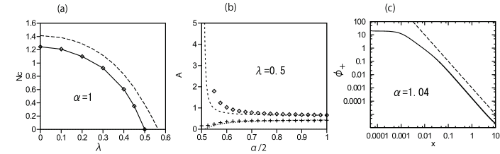
Figure 1: (a) The chain of rhombuses shows the numerically found critical norm $N_{c}$ of the degenerate 1D soliton family as a function of the SOC strength, $\lambda$, at $\alpha=1$. The numerical results are produced by imaginary-time simulations of Eq. (5). The dashed line is the same value as predicted by the VA, as per Eqs. (13) and (12). The numerical and variational values of $N_{c}$ vanish precisely at points (19) and (18), respectively. (b) Chains of rhombuses and crosses show the amplitude of component $|\phi_{+}(x)|$ of the 1D solitons for two fixed values of the norm, $N=1.3$ and $0.8$, respectively, as functions of $\alpha/2$ at fixed $\lambda=0.3$. Dashed lines represent the respective VA-predicted results. (c) An example of a stable 1D soliton, found in the numerical form at $\alpha=1.04$ and $\lambda=1/2$, with total norm $N=1$, is displayed by means of the double-logarithmic plot of $|\phi_{+}(x)|$. The dashed-line fit is $0.001/x^{2}$ (this fit is not valid at still larger values of $|x|$, where the soliton’s tail decays exponentially). In this figure and Fig. 2, the results are presented for $\gamma=0$ in Eq. (5) (no attraction between the two components).

The norm-degenerate family of the 1D solitons existing at $\alpha=1$ and $\lambda<1/2$ is completely unstable. Its relation to nondegenerate families of stable solitons existing at $\alpha>1$ is illustrated by Fig. 1(b), which shows the amplitude of the solitons as a function of $\alpha$ for a fixed SOC strength, $\lambda=0.3$, which is smaller than the one given by Eq. (19) (at $\lambda>1/2$, the solitons definitely do not exist in the limit of $\alpha=1$, as shown above), and for two different fixed norms, $N=0.8$ and $1.3$. Because both are different from the respective value $N_{c}^{\mathrm{(num)}}(\lambda=0.3)\approx 0.9$, see Fig. 1(a), the 1D solitons with these fixed values of $N$ do not exist in the limit of $\alpha=1$. Accordingly, Fig. 1(b) demonstrates that the solitons with $N<N_{c}^{\mathrm{(num)}}(\lambda=0.3)$ suffer delocalization at $\alpha\rightarrow 1$, with the amplitude approaching zero in this limit, while the solitons with $N>N_{c}^{\mathrm{(num)}}(\lambda=0.3)$ suffer collapse (divergence of the amplitude).

Figure 1(c) shows that, at values of $\alpha$ slightly exceeding $1$ (here, $\alpha=1.04$) and $\lambda=1/2$, the 1D soliton exists with tails close to the algebraic shape (comparison to that expression is relevant as $\alpha$ is close to $1$, although Eq. (20) cannot be directly applied because $\alpha$ is not 1). Lastly, Fig. 2 illustrates the stability of a typical 1D soliton with $N=1.3$ at $\alpha=1.4$ and $\lambda=0.3$.

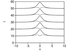
Figure 2: The evolution of $|\phi_{+}(x)|$ and $|\phi_{-}(x)|$ (solid and dashed lines, respectively), produced by simulations of Eq. (5) with $\alpha=1.4$ and $\lambda=0.3$. The norm of this 1D soliton is $N=1.3$.

Thus, the effect of the SOC terms in the 1D system changes the critical norm for the collapse but fails to stabilize the solitons in the critical case of $\alpha=1$. At $\alpha>1$, the effect is not strong either. In particular, additional calculations clearly demonstrate that variation of $\alpha$ does not strongly affect stability of the 1D solitons (details are not displayed here, as they do not convey something remarkable). It is shown below that the SOC terms produce a much more conspicuous impact in the 2D system.

III The 2D system

Following Ref. we , the 2D system of GPEs with the SOC coupling of the Rashba type and the fractional kinetic-energy operator (3) is written, in the scaled form, as

$$i\frac{\partial\phi_{+}}{\partial t} = \frac{1}{2}\left(-\nabla^{2}\right)^{\alpha/2}\phi_{+}-(|\phi_{+}|^{2}+\gamma|\phi_{-}|^{2})\phi_{+}+\lambda\left(\frac{\partial\phi_{-}}{\partial x}-i\frac{\partial\phi_{-}}{\partial y}\right),$$

$$i\frac{\partial\phi_{-}}{\partial t} = \frac{1}{2}\left(-\nabla^{2}\right)^{\alpha/2}\phi_{-}-(|\phi_{-}|^{2}+\gamma|\phi_{+}|^{2})\phi_{-}-\lambda\left(\frac{\partial\phi_{+}}{\partial x}+i\frac{\partial\phi_{+}}{\partial y}\right),$$ (21)

cf. Eq. (5). Note that, except for case of $\alpha=1$, rescaling

$$\left(x,y\right)=\lambda^{-1/(\alpha-1)}\left(\tilde{x},\tilde{y}\right),t=\lambda^{-\alpha/(\alpha-1)}\tilde{t},\phi_{\pm}=\lambda^{\alpha/\left(2(\alpha-1)\right)}\tilde{\phi}_{\pm}$$ (22)

makes it possible to set $\lambda\equiv 1$ in Eq. (21). Accordingly, the norm of the 2D states scales with the variation of the SOC strength as

$$N(\lambda)\equiv\int\int\left(\left|u_{+}\right|^{2}+\left|u_{-}\right|^{2}\right)dxdy=\lambda^{-(2-\alpha)/(\alpha-1)}N(\lambda=1),$$ (23)

where $N(\lambda=1)$ is the norm at the reference point, $\lambda=1$.

Solutions of Eqs. (21) for 2D stationary states with chemical potential $\mu$ are looked for as

$$\phi_{\pm}\left(x,y,t\right)=e^{-i\mu t}u_{\pm}(x,y),$$ (24)

with complex functions $u_{\pm}(x,y)$, cf. the 1D counterpart given by Eq. (6) with real functions $u_{\pm}(x)$. The substitution of ansatz (24) in Eqs. (21) leads to the stationary equations for complex functions $u_{\pm}(x,y)$:

$$\mu u_{+} = \frac{1}{2}\left(-\nabla^{2}\right)^{\alpha/2}u_{+}-(|u_{+}|^{2}+\gamma|u_{-}|^{2})u_{+}+\lambda\left(\frac{\partial u_{-}}{\partial x}-i\frac{\partial u_{-}}{\partial y}\right),$$

$$\mu u_{-} = \frac{1}{2}\left(-\nabla^{2}\right)^{\alpha/2}u_{-}-(|u_{-}|^{2}+\gamma|u_{+}|^{2})u_{-}-\lambda\left(\frac{\partial u_{+}}{\partial x}+i\frac{\partial u_{+}}{\partial y}\right),$$ (25)

cf. the 1D stationary equations (7). Taking into regard definition (3), Eqs. (25) can be derived from the respective Lagrangian:

$$L=\mu\int_{-\infty}^{+\infty}dx\int_{-\infty}^{+\infty}dy\left[\left|u_{+}(x,y)\right|^{2}+\left|u_{-}(x,y)\right|^{2}\right]$$

$$-\frac{1}{2\pi^{2}}\int_{0}^{+\infty}dp\int_{0}^{+\infty}dq(p^{2}+q^{2})^{\alpha/2}\int_{-\infty}^{+\infty}d\xi\int_{-\infty}^{+\infty}d\eta\int_{-\infty}^{+\infty}dx\int_{-\infty}^{+\infty}dy\cos\left[p(x-\xi)+q(y-\eta)\right]$$

$$\times\left[u_{+}^{\ast}(x,y)u_{+}(\xi,\eta)+u_{-}^{\ast}(x,y)u_{-}(\xi,\eta)\right]$$

$$-\lambda\int_{-\infty}^{+\infty}dx\int_{-\infty}^{+\infty}dy\left[u_{+}^{\ast}\frac{\partial u_{-}}{\partial x}+u_{+}\frac{\partial u_{-}^{\ast}}{\partial x}-i\left(u_{+}^{\ast}\frac{\partial u_{-}}{\partial y}-u_{+}\frac{\partial u_{-}^{\ast}}{\partial y}\right)\right]$$

$$+\int_{-\infty}^{+\infty}dx\int_{-\infty}^{+\infty}dy\left[\frac{1}{2}\left(|u_{+}|^{4}+|u_{-}|^{4}\right)+\gamma|u_{+}|^{2}|u_{-}|^{2}\right],$$ (26)

cf. Eq. (8). The integration with respect to $p$ and $q$ in Eq. (26) is reduced from original domains $\left(-\infty,+\infty\right)$ to $\left(0,\infty\right)$, using the symmetry of the domain.

As suggested by Ref. we (which addressed the system with the normal kinetic-energy operator, i.e., $\alpha=2$), we first aim to construct 2D soliton solutions of the SV type. To this end, the following ansatz is adopted:

$$u_{+}=A_{+}\exp(-\beta(x^{2}+y^{2})),u_{-}=A_{-}(x+iy)\exp(-\beta(x^{2}+y^{2})),$$ (27)

which implies vorticities $0$ and $1$ in the components $u_{+}$ and $u_{-}$, respectively, in accordance with the definition of the SV mode. Note that the maximum of component $u_{-}$ of the ansatz, $\left|u_{-}(r)\right|_{\max}=e^{-1/2}A_{-}/\sqrt{2\beta}$, is attained at $r=1/\sqrt{2\beta}$.

The substitution of ansatz (27) in Lagrangian (26) produces the respective effective Lagrangian, cf. Eq. (12):

$$L_{\mathrm{eff}}=\mu N-\frac{\pi\Gamma\left(1+\alpha/2\right)}{2\left(2\beta\right)^{1-\alpha/2}}\left[A_{+}^{2}+\left(1+\frac{\alpha}{2}\right)\frac{A_{-}^{2}}{2\beta}\right]-\frac{\pi\lambda}{\beta}A_{+}A_{-}+\frac{\pi}{8\beta}\left(A_{+}^{4}+\frac{A_{-}^{4}}{8\beta^{2}}+\frac{\gamma A_{+}^{2}A_{-}^{2}}{2\beta}\right),$$ (28)

where the total 2D norm of ansatz (27) is

$$N=\frac{\pi}{2\beta}\left(A_{+}^{2}+\frac{A_{-}^{2}}{2\beta}\right).$$ (29)

Then, for given $\mu$, SV’s parameters are predicted by the Euler-Lagrange equations (cf. Eq. (13)),

$$\frac{\partial L_{\mathrm{eff}}}{\partial A_{\pm}}=\frac{\partial L_{\mathrm{eff}}}{\partial\beta}=0.$$ (30)

Figure 3 presents the most essential results of the analysis for the 2D case with $\gamma=0$ (no nonlinear interaction between components $\phi_{\pm}$ in Eq. (21)). Namely, unlike the 2D version of Eq. (4) with $\alpha\leq 2$, which does not include SOC and generates only completely unstable soliton solutions, Eq. (21) gives rise to stable SVs at $1<\alpha\leq 2$, with norms falling below the respective critical value, viz., $N\,<N_{c}^{\mathrm{(SV)}}(\alpha)$. The dependence of $N_{c}^{\mathrm{(SV)}}$ on $\alpha$, as obtained from the numerical solution (using simulations of Eq. (21) in imaginary time) and VA, is displayed in Fig. 3(a) for $\lambda=0.5$. As it follows from the above argument which demonstrates the peculiarity of the case of $\alpha=1$, $N_{c}^{\mathrm{(SV)}}$ vanishes at $\alpha=1$, which is indeed demonstrated by the numerical results in Fig. 3(a) (while the VA result is inaccurate at $\alpha\rightarrow 1$, as the ansatz (27) is not relevant in this limit). Thus, SV states with a finite amplitude do not exist at $\alpha=1$. On the other hand, for the same case of $\alpha=1$ the solution with the vanishing amplitude can be obtained from the linearized version of Eq. (21). This solution, generated by the imaginary-time simulations of the linearized equations, with periodic boundary conditions fixed for domain $|x|,|y|\leq 10$, is displayed by means of cross sections $\left|\phi_{\pm}\left(x\right)\right|$, drawn through $y=0$, in Fig. 3(b). The effective localization of the solution implies that it is, roughly speaking, similar to periodic states represented by the Jacobi’s elliptic functions with modulus close to $k=1$.

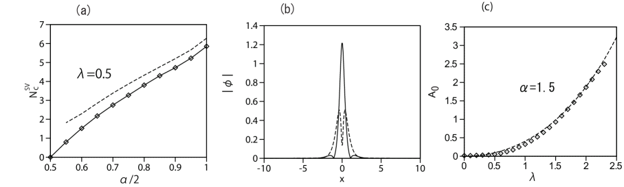
Figure 3: (a) The critical value of the norm of the SV solitons in the 2D system, $N_{c}^{\mathrm{(SV)}}$, as a function of the half Lévy index, $\alpha/2$, at $\lambda=0.5$ for $\gamma=0$ in Eq. (21). At $1<\alpha\leq 2$, the system gives rise to stable SV (semi-vortex) solitons at $N<N_{c}^{\mathrm{(SV)}}$, and to collapse at $N>N_{c}^{\mathrm{(SV)}}$. Here and in panel (c), the chain of rhombuses and dashed line represent, respectively, the numerical findings, obtained from the imaginary-time simulations of Eq. (21), and VA results produced by Eqs. (28) and (30). (b) The cross-section profiles of $|\phi_{+}|$ and $\left|\phi_{-}\right|$ (the solid and dashed lines, respectively), produced at $\lambda=0.5$ and $\alpha=1$ by the numerical solution of the linearized system of size $20\times 20$. Amplitudes of the linear solution are determined by an (arbitrarily adopted) normalization condition $N=1$. (c) The amplitude of the SV solitons (largest value of $|\phi_{+}(x)|$ vs. the SOC strength $\lambda$, at $\alpha=1.5$, $\gamma=0$ and a fixed total norm, $N=0.5$. At small $\lambda$, the dependence is explained by the scaling relation (31) with $\alpha=1.5$, i.e., $A_{0}\sim\sqrt{N}\lambda^{2}$.

The build of the family of stable SV solitons, constructed by means of the numerical solution and VA, is illustrated by Fig. 3(c) for a generic value of the Lévy index, $\alpha=1.5$. In this figure, the SOC strength $\lambda$ is not fixed but varied, to explicitly display the effect of the SOC, while the scaling is used to keep a fixed value of the norm, $N=0.5$ (the mutual scaling of $N$ and $\lambda$ is determined by Eq. (23). It is seen that the SV’s amplitude, $A_{0}(\lambda)$, vanishes at $\lambda\rightarrow 0$ (in agreement with the fact there are no stable 2D solitons in the absence of the SOC in the system). Straightforward analysis of Eqs. (25) and its VA counterpart (30) demonstrates the following scaling relation between the SV’s amplitude, $A_{0}$, its width, $\beta^{-1/2}$ (see Eq. (27)), and $\lambda$, at $\lambda\rightarrow 0$ (cf. Eq. (23):

$$A_{0}\sim\sqrt{N}\lambda^{1/(\alpha-1)},\beta^{-1/2}\sim\lambda^{-1/(\alpha-1)}.$$ (31)

For $\alpha=1.5$, Eq. (31) yields $A_{0}\sim\sqrt{N}\lambda^{2}$, which obviously agrees with the curves plotted in Fig. 3(c).

Further, Fig. 3(c) shows that the amplitude increases with the increase of the SOC strength, up to a maximum value, $\lambda_{\max}\approx 2.4$, above which the SV soliton is destroyed by the collapse. While the VA produces, in the same figure, the amplitude-vs.-$\lambda$ curve which is very close to the numerical counterpart, it does not terminate at $\lambda$ close to $\lambda_{\max}$. Nevertheless, the termination of the soliton family at large $\lambda$ is a natural finding, as the existence of solitons in the system with the SOC terms dominating over the kinetic energy requires the presence of the Zeeman splitting between the components we2 , which is absent in Eqs. (5) and (21).

It is plausible that the stable SV solitons, populating the area beneath the right branch of the $N_{c}^{\mathrm{(SV)}}(\alpha)$ curve in Fig. 3(a), play the role of the system’s ground state, which is missing (formally replaced by the collapsing solution) in the absence of the SOC terms, cf. a similar conclusion made in Ref. we for the usual 2D system with $\alpha=2$. This point calls for a deeper consideration, which is beyond the scope of the present paper.

At values of the norm $N>N_{c}^{\mathrm{(SV)}}$ simulations of Eqs. (21) demonstrate the collapse of the SV, no stationary solitons being possible. At $\alpha<1$, the system does not give rise to solitons either.

The evolution and stability of typical SV solitons in real-time simulations of Eq. (21) with $\gamma=0$ are illustrated in Fig. 4 for (a) $\lambda=1$, $\alpha=1.5$, and $N=1$ and (b) $\lambda=0.4$, $\alpha=1.9$, and $N=5.15$. The latter case represents the 2D system with the Lévy index close to $\alpha=2,$ which corresponds to the system with the usual (non-fractional) kinetic-energy operator, that was considered in Ref. we .

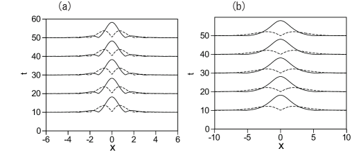
Figure 4: Stable evolution of $|\phi_{+}(x,y)|$ and $|\phi_{-}(x,y)|$ in the SV soliton, plotted in the cross section $y=0$ by solid and dashed lines, respectively, (a) An example for a typical fractional system, with $\lambda=1$, $\alpha=1.5$, and $\gamma=0$ in Eq. (21), and the soliton’s norm $N=1$. (b) The stable evolution in a system close to the regular (non-fractional) one, with $\lambda=0.4$, $\alpha=1.9$, $\gamma=0$, and $N=5.15$.

The above consideration was performed for $\gamma=0$ in Eq. (21), when (as well as for $\gamma<1$, i.e., for the self-attraction of each component stronger than the cross-attraction) the SV is expected to be the dominant species of 2D solitons we . On the other hand, in the usual (non-fractional) system, SVs are unstable at $\gamma>1$, while stable 2D solitons are MM solution, which, as mentioned above, mix the zero-vorticity and vortex terms in each component. The MM represents the ground state of the non-fractional system with $\gamma>1$ we .

In the present case, the MMs may be approximated by the following variational ansatz for the stationary components (see Eq. (24)),

$$u_{+} = A_{1}\exp(-\beta(x^{2}+y^{2}))-A_{2}(x-iy)\exp(-\beta(x^{2}+y^{2})),$$

$$u_{-} = A_{1}\exp(-\beta(x^{2}+y^{2}))+A_{2}(x+iy)\exp(-\beta(x^{2}+y^{2})),$$ (32)

which indeed mixes terms with zero and nonzero vorticities. The substitution of ansatz (32) in Lagrangian (26) yields

$$L_{\mathrm{eff}}=\mu N-\frac{\pi\Gamma\left(2+\alpha/2\right)}{\left(2\beta\right)^{2-\alpha/2}}\left(2\beta A_{1}^{2}+A_{2}^{2}\right)+(1+\gamma)\left(\frac{\pi A_{1}^{4}}{4\beta}+\frac{\pi A_{2}^{4}}{32\beta^{3}}\right)+\frac{\pi A_{1}^{2}A_{2}^{2}}{4\beta^{2}}-\frac{2\lambda\pi A_{1}A_{2}}{\beta},$$ (33)

cf. Eq. (28), where the total norm is $N=\pi[A_{1}^{2}/(\beta)+A_{2}^{2}/(2\beta^{2})]$, cf. Eq. (29). The corresponding variational equations are then derived as per Eq. (30).

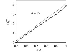
Figure 5: The critical value of the norm of the MM (mixed-mode) solitons in the 2D system, $N_{c}^{\mathrm{(MM)}}$, as a function of the half Lévy index, $\alpha/2$, for fixed $\lambda=0.5$ and $\gamma=2$ in Eq. (21). At $1<\alpha\leq 2$, the system gives rise to stable MM solitons at $N<N_{c}^{\mathrm{(MM)}}$, and to collapse at $N>N_{c}^{\mathrm{(MM)}}$. The chain of rhombuses and dashed line represent, respectively, the numerical findings, obtained from the imaginary-time simulations of Eq. (21), and VA results produced by Eq. (33).

Similar to the SV family, stable 2D solitons of the MM type exist at $\alpha>1$, below the respective critical value of the norm, $N<N_{c}^{\mathrm{(MM)}}$. The numerically found and VA-predicted dependences $N_{c}^{\mathrm{(MM)}}(\alpha)$ are shown in Fig. 5, with $\lambda=0.5$ and $\gamma=2$ fixed in Eq. (21). Note that values of $N_{c}^{\mathrm{(MM)}}$ in Fig. 5 are close to $2/3$ of the respective values of $N_{c}^{\mathrm{(SV)}}$, which are presented, for the same values of $\lambda$ and $\alpha$, in Fig. 3(a). This relation is explained by the same argument which was presented, for $\alpha=2$, in Ref. we : taking into regard that the dominant contribution to the total norm of the SV soliton is produced by the zero-vorticity component, and that the nonlinear interaction between the MM components may be, roughly speaking, absorbed by means of rescaling, $u_{\pm}\rightarrow\left(1+\gamma\right)^{-1/2}u_{\pm}$, an approximate relation between the SV and MM norms is $N^{\mathrm{(MM)}}\approx 2\left(1+\gamma\right)^{-1}N^{\mathrm{(SV)}}$. For $\gamma=2$, it amounts to the above-mentioned norm ratio, $N^{\mathrm{(MM)}}/N^{\mathrm{(SV)}}\approx 2/3$. A similar result, $N^{\mathrm{(MM)}}/N^{\mathrm{(SV)}}\approx 2/(1+\gamma)$, can be obtained for other values of $\gamma>1$, which maintain the MMs as stable states.

If $N<N_{c}^{\mathrm{(MM)}}$ is fixed, while the SOC strength $\lambda$ is varying, the dependence of the MM’s amplitude on $\lambda$ is similar to that for the SVs plotted in Fig. 3(b), i.e., the amplitude vanishes in the limit of $\lambda\rightarrow 0$ according to the same relation (31) which is produced above for the SVs. Figure 6 displays the evolution of components $|\phi_{\pm}(x,y)|$ at $\lambda=1$, $\alpha=1.5$, $\gamma=2$ and $N=0.8$, as produced by real-time simulations of Eq. (21) (note that these parameters correspond to a state located beneath the stability boundary in Fig. 5). The plots clearly demonstrate the structure and stability of the generic MM.

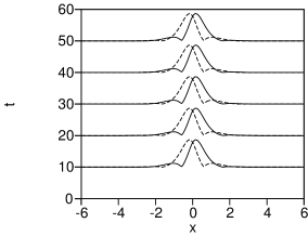
Figure 6: The stable evolution of components $|\phi_{+}(x,y)|$ and $|\phi_{-}(x,y)|$ of a typical MM soliton, shown by solid and dashed lines, respectively, in the cross section of $y=0$. The parameters are $\lambda=1$, $\alpha=1.5$, $\gamma=2$. The total norm of the soliton is $N=0.8$. The input was produced by simulations of Eq. (21) in imaginary time.

At $N>N_{c}^{\mathrm{(MM)}}$, the MM-shaped input leads to the collapse. In the range of $\alpha<1$, where SV solitons do not exist, MM solitons were not found either.

IV Conclusion

This works aims to consider effects of SOC (spin-orbit coupling) in 1D and 2D binary matter waves with the fractional kinetic-energy operator and the usual cubic self- and cross-attractive nonlinearity. This is a model of BEC composed of particles moving by Lévy flights, characterized by the value of the Lévy index, $\alpha<2$ (the normal, non-fractional, kinetic energy corresponds to $\alpha=2$). In the 1D setting, the effect of the SOC is not dramatic, leading to decrease of the norm at which the collapse takes place in the system with $\alpha=1$. Essential effects are predicted in the 2D setting. In that case, the SOC creates regions of stable solitons of the SV (semi-vortex) and MM (mixed-mode) solitons in the interval of $1<\alpha<2$, where the supercritical collapse occurs and no stable modes exist in the absence of SOC. The stable solitons exist at values of the norm below the respective critical values, $N<N_{c}^{\mathrm{(SV,MM)}}$. Amplitudes of the stable solitons in these regions vanish along with SOC strength, $\lambda$, as per Eq. (31).

As an extension of the present analysis, it may be relevant to consider moving solitons and collisions between them. The 2D system may also be used to predict other patterns, such as vortex lattices, cf. Refs. vort-latt -Fukuoka .

References

- (1) Podlubny I, Magin R L and Trymorush I 2017 Niels Henrik Abel and the birth of fractional calculus Fractional Calculus Appl. Anal. 20 1068-1075
- (2) Laskin N 2000 Fractional quantum mechanics and Lévy path integrals Phys. Lett. A 268 298-305
- (3) Dubkov A A, Spagnolo B and Uchaikin V V 2008 Lévy flight superdiffusion: an introduction Int. J. Bifurcat. Chaos 18 2649.
- (4) Laskin N 2018 Fractional Quantum Mechanics (World Scientific, Singapore)
- (5) Riesz M 1949 L’intégrale de Riemann-Liouville et le problème de Cauchy Acta Mathematica 81 1–223, doi:10.1007/BF02395016
- (6) Cai M Li C P 2019 On Riesz derivative Fractional Calculus Appl. Anal. 22 287–301
- (7) Longhi S 2015 Fractional Schrödinger equation in optics Opt. Lett. 40 1117-1120
- (8) Monmayrant A, Weber S and Chatel B 2010 A newcomer’s guide to ultrashort pulse shaping and characterization J. Phys. B: At. Mol. Opt. Phys. 43 103001.
- (9) Kasprzak H 1982 Differentiation of a noninteger order and its optical implementation Appl. Opt. 21 3287-3291
- (10) Davis J A, Smith D A, McNamara D E, Cottrell D M and Campos J 2001 Fractional derivatives - analysis and experimental implementation Appl. Opt. 40 5943-5948
- (11) Stickler B A 2013 Potential condensed-matter realization of space-fractional quantum mechanics: The one-dimensional Lévy crystal Phys. Rev. E 88 012120
- (12) Pinsker F, Bao W, Zhang Y, Ohadi H, Dreismann A, and Baumberg J 2015 Fractional quantum mechanics in polariton condensates with velocity-dependent mass Phys. Rev. B 92 195310
- (13) Zhong W P, Belić M R and Zhang Y 2016 Accessible solitons of fractional dimension Ann. Phys. 368 110–116
- (14) Huang C and Dong L 2016 Gap solitons in the nonlinear fractional Schrödinger equation with an optical lattice Opt. Lett. 41 5636–5639
- (15) Zhang L, He Z, Conti C, Wang Z, Hu Y, Lei D, Li Y and Fan A D 2017 Modulational instability in fractional nonlinear Schrödinger equation Commun. Nonlin. Sci. Numer. Simul. 48, 531–540
- (16) Xiao J, Tian Z, Huang C and Dong L 2018 Surface gap solitons in a nonlinear fractional Schrödinger equation Opt. Exp. 26 2650–2658
- (17) Zeng L and Zeng J 2019 One-dimensional gap solitons in quintic and cubic-quintic fractional nonlinear Schrödinger equations with a periodically modulated linear potential Nonlinear Dyn. 98, 985–995
- (18) Molina M I 2020 The fractional discrete nonlinear Schrödinger equation Phys. Lett. A 384, 126180
- (19) Qiu Y, Malomed B A, Mihalache D, Zhu X, Zhang L and He Y 2020 Soliton dynamics in a fractional complex Ginzburg-Landau model Chaos, Solitons and Fractals 131 109471
- (20) Li P, Malomed B A and Mihalache D 2020 Vortex solitons in fractional nonlinear Schrödinger equation with the cubic-quintic nonlinearity Chaos Solitons & Fractals 137 109783
- (21) Wang Q and Liang G 2020 Vortex and cluster solitons in nonlocal nonlinear fractional Schrödinger equation J. Optics 22 055501
- (22) Li P, Malomed B A, and Mihalache D 2020 Metastable soliton necklaces supported by fractional diffraction and competing nonlinearities Opt. Exp. 28 34472-34488
- (23) Qiu Y, Malomed B A, Mihalache D, Zhu X, Peng X and He Y 2020 Stabilization of single- and multi-peak solitons in the fractional nonlinear Schrödinger equation with a trapping potential Chaos, Solitons & Fractals 140 110222
- (24) Li P, Malomed B A and Mihalache D 2020 Symmetry breaking of spatial Kerr solitons in fractional dimension Chaos Solitons & Fractals 132 109602
- (25) Li P and Dai C 2020 Double loops and pitchfork symmetry breaking bifurcations of optical solitons in nonlinear fractional Schrödinger equation with competing cubic-quintic nonlinearities Ann. Phys. (Berlin) 532 2000048
- (26) Li P, Li R and Dai C 2021 Existence, symmetry breaking bifurcation and stability of two-dimensional optical solitons supported by fractional diffraction Opt. Exp. 29, 3193–3210
- (27) Zeng L, Mihalache D, Malomed B A, Lu X, Cai Y, Zhu Q, and Li J 2021 Families of fundamental and multipole solitons in a cubic-quintic nonlinear lattice in fractional dimension Chaos Sol. Fract. 144 110589
- (28) Zeng L, Zhu Y, Malomed B A, Mihalache D, Wang Q, Long H, Cai Y, Lu X and Li J 2022 Quadratic fractional solitons Chaos, Solitons & Fractals 154 111586
- (29) Malomed B A 2021 Optical solitons and vortices in fractional media: A mini-review of recent results Photonics 8 353
- (30) Chen M N, Zeng S H, Lu D Q, Hu W and Guo Q 2018, Optical solitons, self-focusing, and wave collapse in a space-fractional Schrödinger equation with a Kerr-type nonlinearity Phys. Rev. E 98 022211
- (31) Sulem C and Sulem P L 1999 The Nonlinear Schrödinger Equation: Self-focusing and Wave Collapse (Springer, Berlin).
- (32) Fibich G 2015 The Nonlinear Schrödinger Equation: Singular Solutions and Optical Collapse (Springer, Heidelberg)
- (33) Sakaguchi H, Li B, and Malomed B A 2014 Creation of two-dimensional composite solitons in spin-orbit-coupled self-attractive Bose-Einstein condensates in free space Phys. Rev. E 89 032920
- (34) Sakaguchi H, Sherman E Ya, and Malomed B A 2016 Vortex solitons in two-dimensional spin-orbit coupled Bose-Einstein condensates: Effects of the Rashba-Dresselhaus coupling and the Zeeman splitting Phys. Rev. E 94 032202
- (35) Malomed B A 2018 Creating solitons by means of spin-orbit coupling EPL 122 36001
- (36) Zhai H 2015 Degenerate quantum gases with spin–orbit coupling: a review Rep. Prog. Phys. 78 026001
- (37) Zhang Y, Mossman M E, Busch T, Engels P and Zhang C 2016 Properties of spin–orbit-coupled Bose–Einstein condensates Front. Phys. 11 118103
- (38) Zhang Y, Mao L, and Zhang C 2012 Mean-field dynamics of spin-orbit coupled Bose-Einstein condensates Phys. Rev. Lett. 108 035302
- (39) Chiao R Y, Garmire E and Townes C H 1964 Self-trapping of optical beams Phys. Rev. Lett. 13 479–482
- (40) Desaix M, Anderson D and Lisak M 1991 Variational approach to collapse of optical pulses J. Opt. Soc. Am. B 8 2082-2086
- (41) Sakaguchi H and Malomed B A 2016 One- and two-dimensional solitons in -symmetric systems emulating spin–orbit coupling New J. Phys. 18, 105005
- (42) Zhou X F, Zhou J, Wu, and Wu C J 2011 Vortex structures of rotating spin-orbit-coupled Bose-Einstein condensates Phys. Rev. A 84, 063624
- (43) Xu Z F, Kawaguchi Y, You L, and Ueda M 2012 Symmetry classification of spin-orbit-coupled spinor Bose-Einstein condensates Phys. Rev. A 86, 033628
- (44) Ruokokoski E, Huhtamaki J A M, and Mottonen M 2012 Stationary states of trapped spin-orbit-coupled Bose-Einstein condensates Phys. Rev. A 86, 051607
- (45) H. Sakaguchi and B. Li 2013 Vortex lattice solutions to the Gross-Pitaevskii equation with spin-orbit coupling in optical lattices Phys. Rev. A 87, 015602