Optimization with Access to Auxiliary Information

Abstract

We investigate the fundamental optimization question of minimizing a target function $f({\bm{x}})$, whose gradients are expensive to compute or have limited availability, given access to some auxiliary side function $h({\bm{x}})$ whose gradients are cheap or more available. This formulation captures many settings of practical relevance, such as i) re-using batches in SGD, ii) transfer learning, iii) federated learning, iv) training with compressed models/dropout, etc. We propose two generic new algorithms that apply in all these settings and prove that we can benefit from this framework using only an assumption on the Hessian similarity between the target and side information. A benefit is obtained when this similarity measure is small, we also show a potential benefit from stochasticity when the auxiliary noise is correlated with that of the target function.

1 Introduction

Motivation.

Stochastic optimization methods such as SGD (Robbins & Monro, 1951) or Adam (Kingma & Ba, 2014) are arguably at the core of the success of large-scale machine learning (LeCun et al., 2015; Schmidhuber, 2015). This success has led to significant (perhaps even excessive) research efforts dedicated to designing new variants of these methods (Schmidt et al., 2020). In all these methods, massive datasets are collected centrally on a server, and immense parallel computational resources of a data center are leveraged to perform training (Goyal et al., 2017; Brown et al., 2020). Meanwhile, modern machine learning is moving away from this centralized training setup with new paradigms emerging, such as i) distributed/federated learning, ii) semi-supervised learning, iii) personalized/multi-task learning, iv) model compression, etc. Relatively little attention has been devoted to these more practical settings from the optimization community. In this work, we focus on extending the framework and tools of stochastic optimization to bear on these novel problems.

At the heart of these newly emergent training paradigms lies the following fundamental optimization question: We want to minimize a target loss function $f({\bm{x}})$, but computing its stochastic gradients is either very expensive or unreliable due to the limited amount of data. However, we assume having access to some auxiliary loss function $h({\bm{x}})$ whose stochastic gradient computation is relatively cheaper or more reliable. For example, in transfer learning, $f({\bm{x}})$ would represent the downstream task we care about and for which we have very little data available, whereas $h({\bm{x}})$ would be the pretraining task for which we have plenty of data (Yosinski et al., 2014). Similarly, in semi-supervised learning, $f({\bm{x}})$ would represent the loss over our clean labeled data, whereas $h({\bm{x}})$ represents the loss over unlabeled or noisily labeled data (Chapelle et al., 2009). Our challenge then is the following question:

How can we leverage an auxiliary $h({\bm{x}})$ to speed up the optimization of our target loss function $f({\bm{x}})$?

Of course, if $f({\bm{x}})$ and $h({\bm{x}})$ are completely unrelated, our task is impossible and we cannot hope for any speedup over simply running standard stochastic optimization methods (e.g. SGD) on $f({\bm{x}})$. So an additional question before us is to define and take advantage of useful measures of similarity between $f({\bm{x}})$ and $h({\bm{x}})$.

Contributions. The main results in this work are

• We formulate the following as stochastic optimization with auxiliary information: i)Re-using batches in SGD, ii) Semi-supervised learning, iii) transfer learning, iv) Federated Learning, v) personalized learning, and iv) training with sparse models.

• We show a useful and simple trick (Eq3) to construct biased gradients using gradients from an auxiliary function.

• Based on the above trick, We design a biased gradient estimator of $f({\bm{x}})$ which reuses stochastic gradients of $f({\bm{x}})$ and combines it with gradients of $h({\bm{x}})$.

• We then use this estimator to develop algorithms for minimizing smooth non-convex functions. Our methods improve upon known optimal rates that don’t use any side information.

Related work. Optimizing one function $f$ while having access to another function $h$ (or its gradients) is an important idea that has been used in special cases in machine learning and optimization communities. To the best of our knowledge, this problem was never considered in all of its generality before this time. For this reason, we can only cite works that used this idea indirectly. Lately, masked training of neural networks was considered for example in (Alexandra et al., 2019; Amirkeivan et al., 2021), this approach can be understood as a special case of our framework, where the auxiliary information is given by the sub-network (or mask). In distributed optimization, (Shamir et al., 2013) define sub-problems based on available local information, the main problem with this approach is that the defined sub-problems need to be solved precisely in theory and to high precision in practice. In Federated Learning (Konecny et al., 2016; McMahan et al., 2017a; Mohri et al., 2019), the local functions (constructed using local datasets) can be seen as side information. Applying our framework recuperates an algorithm close to MiMe (Karimireddy et al., 2020a). In personalization, Chayti et al. (2021) study the collaborative personalization problem where one user optimizes its loss by using gradients from other available users (that are willing to collaborate), again these collaborators can be seen as side information, one drawback of the approach in (Chayti et al., 2021) is that they need the same amount of work from the main function and the helpers, in our case we alleviate this by using the helpers more.
There is also auxiliary learning (Baifeng et al., ; Aviv et al., ; Xingyu et al., ) that is very similar to what we are proposing in this work. Auxiliary learning also has the goal of learning one given task using helper tasks, however, all these works come without any theoretical convergence guarantees, furthermore, our approach is more general.
The proposed framework is general enough to include all the above problems and more. More importantly, we don’t explicitly make assumptions on how the target function $f$ is related to the auxiliary side information $h$ (potentially a set of functions) like in Distributed optimization or Federated learning where we assume $f$ is the average of the side-information $h$. Also, it is not needed to solve the local problems precisely as expected by DANE (Shamir et al., 2013).

2 General Framework

Our main goal is to solve the following optimization problem:

$$\min_{{\bm{x}}\in\mathbb{R}^{d}}f({\bm{x}})\,,$$ (1)

and we suppose that we have access to an auxiliary function $h({\bm{x}})$ that is related to $f$ in a sense that we don’t specify at this level.

Specifically, we are interested in the stochastic optimization framework. We assume that the target function is of the form $f({\bm{x}}):=\mathbb{E}_{\xi_{f}}\big{[}f({\bm{x}};\xi_{f})\big{]}$ over ${\bm{x}}\in\mathbb{R}^{d}$ while the auxiliary function has the form $h({\bm{x}}):=\mathbb{E}_{\xi_{h}}\big{[}h({\bm{x}};\xi_{h})\big{]}$ defined over the same parameter space. We will refer to these two functions simply as $f$ and $h$ and stress that they should not be confused with $f(\cdot;\zeta_{f})$ and $h(\cdot;\zeta_{h})$. It is evident that if both functions $f$ and $h$ are unrelated, we can’t hope to benefit from the auxiliary information $h$. Hence we need to assume some similarity between $f$ and $h$. In our case, we propose to use the hessian similarity (defined in assumption 3.3).

Many optimization algorithms can be framed as sequential schemes that, starting from an estimate ${\bm{x}}$ of the minimizer, compute the next (hopefully better estimate) ${\bm{x}}^{+}$ by solving a potentially simpler problem

$${\bm{x}}^{+}\in arg\min_{{\bm{z}}\in\mathbb{R}^{d}}\{\hat{f}({\bm{z}};{\bm{x}})+\lambda R({\bm{z}};{\bm{x}})\}\,,$$ (2)

where $\hat{f}(\cdot;{\bm{x}})$ is an approximation of $f$ around the current state ${\bm{x}}$, $R({\bm{z}};{\bm{x}})$ is a regularization function that measures the quality of the approximation and $\lambda$ is a parameter that trades off the two terms.

For example, the gradient descent algorithm is obtained by choosing $\hat{f}({\bm{z}};{\bm{x}})=f({\bm{x}})+\nabla f({\bm{x}})^{\top}({\bm{z}}-{\bm{x}})$, $R({\bm{z}};{\bm{x}})=\frac{1}{2}\|{\bm{z}}-{\bm{x}}\|_{2}^{2}$ and $\lambda=\frac{1}{\eta}$ where $\eta$ is the stepsize. Mirror descent uses the same approximation $\hat{f}$ but a different regularizer $R({\bm{z}};{\bm{x}})=\mathcal{D}_{\phi}({\bm{z}};{\bm{x}})$ where $\mathcal{D}_{\phi}$ is the Bregman divergence of a certain strongly-convex function $\phi$.

We take inspiration from this approach in this work. However, we would like to take advantage of the existence of the auxiliary function $h$. We will mainly focus on first-order approximations of $f$ throughout this work, we will also fix the regularization function $R({\bm{z}};{\bm{x}})=\frac{1}{2}\|{\bm{z}}-{\bm{x}}\|_{2}^{2}$, we note that our ideas can be easily adapted to other choices of $R$ and more involved approximations of $f$.

For any function $h$, we can always write $f$ as

$$f({\bm{z}}):=\underbrace{h({\bm{z}})}_{\text{cheap}}\;+\;\underbrace{f({\bm{z}})-h({\bm{z}})}_{\text{expensive}}\,,$$

we term the first term as “cheap" but this should not be understood in a strict manner, it can for example also mean more available.

A very straightforward approach is to use $f$ whenever it is available and use $h$ as its proxy whenever it is not, we term this approach the naive approach. This is equivalent to simply ignoring (in other words using a zeroth-order approximation of) the “expensive" part.

A more involved strategy is to approximate the “expensive" part $f({\bm{z}})-h({\bm{z}})$ as well but not as much as the “cheap" part $h({\bm{z}})$. We can do this by approximating $f({\bm{z}})-h({\bm{z}})$ around ${\bm{x}}$ ( a global state, or a snapshot, the idea is that it is the state of $f$) and approximating $h({\bm{z}})$ around ${\bm{y}}$ (a local state in the sense that it is updated by $h$). Doing this we get the following update rule

$${\bm{y}}^{+}\in arg\min_{{\bm{z}}\in\mathbb{R}^{d}}\{\hat{f}({\bm{z}};{\bm{y}},{\bm{x}})+\frac{1}{2\eta}\|{\bm{z}}-{\bm{y}}\|_{2}^{2}\}\,,$$

where $\hat{f}({\bm{z}};{\bm{y}},{\bm{x}}):=h({\bm{y}})+f({\bm{x}})-h({\bm{x}})+(\nabla h({\bm{y}})-\nabla h({\bm{x}})+\nabla f({\bm{x}}))^{\top}({\bm{z}}-{\bm{x}})$.

This is equivalent to

$${\bm{y}}^{+}={\bm{y}}-\eta(\nabla h({\bm{y}})-\nabla h({\bm{x}})+\nabla f({\bm{x}}))$$ (3)

We will refer to (3) as a local step because it uses a new gradient of $h$ to update the state. The idea is that for each state ${\bm{x}}$ of $f$, we perform a number of local steps, then update the state ${\bm{x}}$ based on the last “local" steps.

Control variates and SVRG. (3) can be understood as a generalization of the control variate idea used in SVRG (Johnson & Zhang, 2013). To optimize a function $f({\bm{x}}):=\frac{1}{n}\sum_{i=1}^{n}f_{i}({\bm{x}})$, SVRG uses the modified gradient ${\bm{g}}_{SVRG}=\nabla f_{i}({\bm{y}})-\nabla f_{i}({\bm{x}})+\nabla f({\bm{x}})$ where ${\bm{x}}$ is a snapshot that is updated less frequently and $i$ is sampled randomly so that this new gradient is still unbiased. The convergence of SVRG is guaranteed by the fact that the “error” of this new gradient is $\mathbb{E}\|{\bm{g}}_{SVRG}-\nabla f({\bm{x}})\|_{2}^{2}=\mathcal{O}(\|{\bm{y}}-{\bm{x}}\|_{2}^{2})$ so that if ${\bm{y}}-{\bm{x}}\rightarrow 0$, then convergence is guaranteed without needing to take small step-sizes. The main idea of our work is to use instead of $f_{i}$ another function $h$ that is related to $f$, this means using a gradient ${\bm{g}}=\nabla h({\bm{y}})-\nabla h({\bm{x}})+\nabla f({\bm{x}})$, then if we can still guarantee that the error is $\mathcal{O}(\|{\bm{y}}-{\bm{x}}\|_{2}^{2})$ everything should still work fine.

What if we can’t access the true gradient of $f$? when $f$ is not a finite average, we can’t access its true gradient, in this case, we propose replacing the “correction” $\nabla f({\bm{x}})-\nabla h({\bm{x}})$ by a quantity ${\bm{m}}_{f-h}$ that is a form of momentum (takes into account past observed gradients of $f-h$), the idea of using momentum is used to stabilize the estimate of the quantity $\nabla f({\bm{x}})-\nabla h({\bm{x}})$ as momentum can be used to reduce the variance. Specifically, we use ${\bm{g}}=\nabla h({\bm{y}})+{\bm{m}}_{f-h}$. We note that for this estimate we have $\mathbb{E}\|{\bm{g}}-\nabla f({\bm{y}})\|_{2}^{2}=\mathcal{O}(\|{\bm{y}}-{\bm{x}}\|_{2}^{2}+\|{\bm{m}}_{f-h}-\nabla f({\bm{x}})+\nabla h({\bm{x}})\|_{2}^{2})$ which means that ${\bm{g}}$ approximates $\nabla f({\bm{y}})$ as long as ${\bm{y}}$ is not far from ${\bm{x}}$ and ${\bm{m}}_{f-h}$ is a good estimate of the quantity $\nabla f({\bm{x}})-\nabla h({\bm{x}})$.

Local steps or a subproblem? we note that another possible approach is instead of defining local steps based on $h$, to define a subproblem that gives the next estimate of $f$ directly by solving

$${\bm{x}}^{+}\in arg\min_{{\bm{y}}\in\mathbb{R}^{d}}\{h({\bm{y}})+{\bm{m}}_{f-h}^{\top}({\bm{y}}-{\bm{x}})+\frac{1}{2\eta}\|{\bm{y}}-{\bm{x}}\|_{2}^{2}\}\;.$$ (4)

Our results can be understood as approximating a solution to this sub-optimization problem (4).

Notation. For a given function $J$, we denote ${\bm{g}}_{J}(\cdot,\xi_{J})$ an unbiased estimate of the gradient of $J$ with randomness $\xi_{J}$.

General meta-algorithm. Based on the discussion above, we propose the (meta)-Algorithm 1: at the beginning of each round $t$, we have an estimate ${\bm{x}}^{t-1}$ of the minimizer. We sample a new $\zeta_{f-h}$ and compute ${\bm{g}}_{f-h}({\bm{x}}_{t-1},\zeta_{f-h})$ a noisy unbiased estimate of the gradient of $f-h$, we then update ${\bm{m}}_{f-h}^{t}$ a momentum of $f-h$. We transfer both ${\bm{x}}^{t-1}$ and ${\bm{m}}_{f-h}^{t}$ to the helper $h$ which uses both to construct a set of biased gradients ${\bm{d}}^{t}_{k}$ of $\nabla f({\bm{y}}^{t}_{k-1})$ that are updated by $h$ . These biased gradients are then used to update the “local" states ${\bm{y}}^{t}_{k}$, then $f$ updates its own state ${\bm{x}}^{t}$ based on the last local states ${\bm{y}}^{t}_{0\leq k\leq K}$. Throughout this work, we simply take ${\bm{x}}_{t}={\bm{y}}^{t}_{K}$.

0:  ${\bm{x}}_{0}$, $\eta$, $T$, $K$

  for $t=1$ to $T$ do

     sample ${\bm{g}}_{f-h}({\bm{x}}^{t-1},\xi^{t}_{f-h})\approx\nabla f({\bm{x}}^{t-1})-\nabla h({\bm{x}}^{t-1})$

     update ${\bm{m}}_{f-h}^{t}\approx\nabla f({\bm{x}}^{t-1})-\nabla h({\bm{x}}^{t-1})$ § momentum

     define ${\bm{y}}^{t}_{0}={\bm{x}}^{t-1}$

     for $k=1$ to $K$ do

        sample ${\bm{g}}_{h}({\bm{y}}^{t}_{k-1},\xi^{t,k}_{h})\approx\nabla h({\bm{y}}^{t}_{k-1})$

        use it and ${\bm{m}}^{t}$ to form ${\bm{d}}^{t}_{k}\approx\nabla f({\bm{y}}^{t}_{k-1})$

        ${\bm{y}}^{t}_{k}={\bm{y}}^{t}_{k-1}-\eta{\bm{d}}^{t}_{k}$

     end for

     update ${\bm{x}}^{t}$

  end for

Algorithm 1 stochastic optimization of $f$ with access to the auxiliary $h$

For our purposes we can take ${\bm{d}}^{t}_{k}={\bm{g}}_{h}({\bm{y}}^{t}_{k-1},\xi^{t,k}_{h})+{\bm{m}}^{t}_{f-h}$ which should be a good approximation of $\nabla f({\bm{y}}^{t}_{k-1})$ and ${\bm{m}}^{t}_{f-h}$ is a momentum of $f-h$, we will consider two options: classical momentum or MVR (for momentum based variance reduction).

Decentralized auxiliary information. More generally, we can assume having access to $N$ auxiliary functions $h_{i}({\bm{x}}):=\mathbb{E}_{\xi_{h_{i}}}\big{[}h_{i}({\bm{x}};\xi_{h_{i}})\big{]}$. While we can treat this case by taking $h=(1/N)\sum_{i=1}^{N}h_{i}$, we propose a more interesting solution that will also work if the helpers $h_{i}$ are decentralized and cannot live in the same server. In this case, we can sample a set $S^{t}$ of helpers, each $h_{i}\in S^{t}$ will do the updates exactly as in Algorithm1, but this time ${\bm{x}}^{t}$ will be constructed using all $\{{\bm{y}}^{t}_{i,K},i\in S^{t}\}$. In our case, we propose to use the average ${\bm{x}}^{t}=(1/S)\sum_{i\in S^{t}}{\bm{y}}^{t}_{i,K}$ .

3 Algorithms and Results

We discuss here some special cases of Algorithm 1 based on choices of ${\bm{m}}^{t}_{f-h}$ and ${\bm{d}}^{t}_{k}$ which we kept a little bit vague purposefully.

We will consider mainly two approaches, the first one we call the Naive approach and the second one we refer to as Bias correction.

We remind the reader that we can take ${\bm{d}}^{t}_{k}={\bm{g}}_{h}({\bm{y}}^{t}_{k-1},\xi^{t,k}_{h})+{\bm{m}}^{t}_{f-h}$.

Naive approach. This approach is exactly as it is suggested by its name, naive, it simply ignores the part $f-h$ or in other words ${\bm{m}}^{t}_{f-h}=0$ . The main idea is to use gradients (or gradient estimates) of $f$ whenever they are available and use gradients of $h$ when gradients of $f$ are not available. In our case, we alternate between one step using a gradient of $f$ and $(K-1)$-steps using gradients of $h$ without any correction. We will show that this approach suffers heavily from the bias between the gradients of $f$ and $h$. It is worth noting that in federated learning, this approach corresponds to Federated averaging (McMahan et al., 2017a).
Bias correction. In the absence of noise, this approach simply implements (3). Specifically, the inner loop in Algorithm 1 does this

$${\bm{y}}^{t}_{k}={\bm{y}}^{t}_{k-1}-\eta(\underbrace{\nabla h({\bm{y}}^{t}_{k-1})-\nabla h({\bm{x}}^{t-1})+\nabla f({\bm{x}}^{t-1})}_{:={\bm{d}}^{t}_{k}})$$

In the noisy case (when we can only have access to noisy gradients of $f$) we approximate the above step in the following way:

$${\bm{y}}^{t}_{k}={\bm{y}}^{t}_{k-1}-\eta(\underbrace{{\bm{g}}_{h}({\bm{y}}^{t}_{k-1},\xi^{t}_{k-1})+{\bm{m}}_{f-h}^{t}}_{:={\bm{d}}^{t}_{k}})\;,$$

where ${\bm{m}}_{f-h}^{t}$ is a momentum of $f-h$. We consider two methods for defining this momentum:

$${\bm{m}}_{f-h}^{t} =(1-a){\bm{m}}_{f-h}^{t-1}+a{\bm{g}}_{f-h}({\bm{x}}^{t-1},\xi^{t-1}_{f-h})\qquad(\textbf{AuxMom})$$ (5)

$${\bm{m}}_{f-h}^{t} =(1-a){\bm{m}}_{f-h}^{t-1}+a{\bm{g}}_{f-h}({\bm{x}}^{t-1},\xi^{t}_{f-h})$$

$$+(1-a)\big{(}{\bm{g}}_{f-h}({\bm{x}}^{t-1},\xi^{t}_{f-h})-{\bm{g}}_{f-h}({\bm{x}}^{t-2},\xi^{t-2}_{f-h})\big{)}\qquad(\textbf{AuxMVR})$$ (6)

AuxMom simply uses the classical momentum, whereas AuxMVR uses the momentum-based variance reduction technique introduced in (Cutkosky & Orabona, 2019).

Assumptions. To analyze our algorithms, we will make the following assumptions on the target $f$ and the helper $h$.

Assumption 3.1.

(Smoothness.) We assume that $f$ has $L$-Lipschitz gradients and satisfy

$$\|\nabla f({\bm{x}})-\nabla f({\bm{y}})\|_{2}\leq L\|{\bm{x}}-{\bm{y}}\|_{2}\,.$$

Assumption 3.2.

(Variance.) The stochastic gradients ${\bm{g}}_{f}({\bm{x}};\zeta_{f})$, ${\bm{g}}_{h}({\bm{x}};\zeta_{h})$ and ${\bm{g}}_{f-h}({\bm{x}};\zeta_{f-h})$ are unbiased, and satisfy

$$\mathbb{E}_{\zeta_{J}}\|{\bm{g}}_{J}({\bm{x}};\zeta_{J})-\nabla J({\bm{x}})\|_{2}^{2}\leq\sigma_{J}^{2}\,,J\in\{f,h,f-h\}\,.$$

In Assumption 3.2 we assume that we directly have access to unbiased gradient estimates of $f-h$. This does not restrict in any way our work since ${\bm{g}}_{f}-{\bm{g}}_{h}$ is such an estimate, however, this last estimate has a variance of $\sigma_{f-h}^{2}=\sigma_{f}^{2}+\sigma_{h}^{2}$, in general, it is possible to have a correlated estimate such that $\sigma_{f-h}^{2}<\sigma_{f}^{2}+\sigma_{h}^{2}$.

Assumption 3.3.

Hessian similarity. Finally, we will assume that for some $\delta\in[0,2L]$ we have

$$\|\nabla^{2}f({\bm{x}})-\nabla^{2}h({\bm{x}})\|_{2}\leq\delta\,.$$

Note that if $h(\cdot)$ is also smooth (satisfies Assumption 3.1), then we would have Hessian similarity with $\delta\leq 2L$ since

$$\|\nabla^{2}f({\bm{x}})-\nabla^{2}h({\bm{x}})\|_{2}\leq\|\nabla^{2}f({\bm{x}})\|_{2}+\|\nabla^{2}h({\bm{x}})\|_{2}\leq 2L\,.$$

As sanity checks, $h=0$ corresponds to $\delta=L$ (this case should not lead to any benefit), and $h=f$ gives $\delta=0$, we will consider these two cases to verify our convergence rates.

Relaxing the Hessian similarity. Jingzhao et al. propose a generalized smoothness assumption where the norm of the Hessian can grow with the norm of the gradient. We believe it is possible to extend our theory to accommodate such an assumption. In the same spirit, we can let $\|\nabla^{2}f({\bm{x}})-\nabla^{2}h({\bm{x}})\|_{2}$ grow with $\|\nabla f({\bm{x}})\|_{2}$. More important than this would be to find similarity measures that apply to some of the potential applications that we cite in Section 5.

4 Results

We start by showing the convergence rate of the naive approach is dominated by the gradient bias. Then show the convergence rate of our momentum variant AuxMom that will be compared to SGD/GD. We will also state the convergence rate of our AuxMVR variant and compare it to MVR/GD.
Notation. We assume $f$ is bounded from below and denote $f^{\star}=\underset{{\bm{x}}\in\mathbb{R}^{d}}{\inf}f({\bm{x}})$.
Remark. We would like to note that while we state our results for the case of one helper $h$, they also apply without needing any additional assumption when we have $N$ decentralized helpers $h_{1},\ldots,h_{N}$ from which we sample $S=1$ helper at random. In the case where $S>1$, we need an additional weak-convexity assumption to deal with the averaging performed at the end of each step; this general case is treated in Appendix C.4.

4.1 Naive approach

In this section, we show the convergence results using the naive approach that uses a gradient of $f$ followed by $K-1$ gradients of $h$. For the analysis of this case (and only of this case), we need to make an assumption on the gradient bias between $f$ and $h$.

Assumption 4.1.

The gradient bias between $f$ and $h$ is $(m,\zeta^{2})-$bounded: $\forall{\bm{x}}\in\mathbb{R}^{d}\;:\|\nabla f({\bm{x}})-\nabla h({\bm{x}})\|_{2}^{2}\leq m\|\nabla f({\bm{x}})\|_{2}^{2}+\zeta^{2}.$

There exists $f$ and $h$ satisfying assumptions 3.1,3.2,4.1 with $\sigma_{f}=0$ such that $\frac{1}{KT}\sum_{t=1}^{T}\|\nabla f({\bm{x}}^{t-1})\|_{2}^{2}=\Omega(\zeta^{2})$. Using the biased SGD analysis in (Ajalloeian & Stich, 2020) it is easy to prove an upper bound, but we only need a lower bound for our purposes. Theorem 4.1 shows that this naive approach cannot guarantee convergence to less than $\zeta^{2}$ (up to some constant).
Note. Theorem 4.1 does not apply to Federated averaging since in this case $f$ is directly related to the helpers. However, heterogeneity and client drift (similar to gradient bias) are known to limit the performance of FedAVG. Hence approaches that try to reduce it like (Karimireddy et al., 2020b; a)

In the following, we will show that our two proposed algorithms solve this bias problem.

4.2 Momentum based approach

We consider the instance of Algorithm 1 with the momentum choice in (5). For clarity, a detailed Algorithm can be found in the Appendix Algorithm 3.

Convergence rate. We prove the following theorem that gives the convergence rate of this algorithm in the non-convex case. Under assumptions A3.1, 3.2,3.3. For $a=32\delta K\eta$
and $\eta=\min\bigg{(}\frac{1}{L},\frac{1}{192\delta K},\sqrt{\frac{\tilde{F}}{128LKT\beta\sigma_{f}^{2}}}\bigg{)}\,,$ we have :

$$\frac{1}{KT}\sum_{t=1}^{T}\sum_{k=0}^{K-1}\mathbb{E}\big{[}\|\nabla f({\bm{y}}^{t}_{k})\|_{2}^{2}\big{]}=\\ \mathcal{O}\bigg{(}\sqrt{\frac{L\tilde{F}\sigma_{f}^{2}\beta}{T}}+\frac{(L+\delta K)\tilde{F}}{KT}\bigg{)}\,.$$

where $\tilde{F}=F^{0}+\frac{E^{0}}{\delta}$, $F^{0}=f({\bm{x}}^{0})-f^{\star}$, $E^{0}=\mathbb{E}[\|{\bm{m}}^{0}-\nabla f({\bm{x}}^{0})+\nabla h({\bm{x}}^{0})\|_{2}^{2}]$ and $\beta=\mathcal{O}\big{(}\frac{\delta}{L}\frac{\sigma_{f-h}^{2}}{\sigma_{f}^{2}}+\frac{1}{K}(1+\frac{\delta}{L})\frac{\sigma_{h}^{2}}{\sigma_{f}^{2}}$) . Note. We note the term $E^{0}$ in the definition of $\tilde{F}$, we show in the appendix how to get rid of this term $E^{0}$ by making it $\mathcal{O}(1/T)$, for this reason, we may consider $\tilde{F}=F^{0}$.
For simplicity, we take $\sigma_{h}=\sigma_{f}$ (it is reasonable to assume the two quantities of the same order).

Sanity checks. For $h=f$, we have $\delta=0$, and it is easy to see that we get the rate of $KT$-steps of SGD. For $h=0$ we have $\delta=L$, in this case, we don’t gain anything as should be the case.
We will compare this rate to that of SGD under the same amount of work asked from $f$: $\mathcal{O}\bigg{(}\sqrt{\frac{LF^{0}\sigma_{f}^{2}}{T}}+\frac{LF^{0}}{T}\bigg{)}$.
When do we gain from the helper? (Noiseless case.) for $\sigma_{f}=\sigma_{h}=0$, we have the rate $\mathcal{O}(LF^{0}/(KT)+\delta F^{0}/T)$, we compare this to $\mathcal{O}(LF^{0}/T)$ the expected rate had we only used gradients of $f$. This means that we gain a multiplicative factor of $1/K+\delta/L$, which means we need $\delta/L\ll 1$ (very small) to neglect it. however, there is another consequence: for $K\leq L/\delta$ the rate is $\mathcal{O}(LF^{0}/(KT))$, in other words, it is as if we were using $K$ gradients of $f$ instead of only $1$ and $K-1$ gradients of $h$.(Noisy case.) We see that in the dominant term we have the factor $\beta$ that multiplies the variance term $\sigma_{f}^{2}$ that we have in SGD (when we don’t use the helper $h$), the smaller $\beta$ the better, this is the case in general if $\delta/L$, $\sigma_{h}^{2}/\sigma_{f}^{2}$ are small and $\sigma_{f-h}^{2}/\sigma_{f}^{2}$. We also notice a small gain from $K$.

Specifically, $\beta=\mathcal{O}\big{(}\frac{\delta}{L}\frac{\sigma_{f-h}^{2}}{\sigma_{f}^{2}}+\frac{1}{K}(1+\frac{\delta}{L})\frac{\sigma_{h}^{2}}{\sigma_{f}^{2}}$) is constituted of two terms, the first one $\frac{\delta}{L}\frac{\sigma_{f-h}^{2}}{\sigma_{f}^{2}}$ suggests that we may benefit if $\delta\ll L$ or if $\sigma_{f-h}^{2}\ll\sigma_{f}^{2}$, we get the latter if our gradient estimates of $f$ are positively correlated with the gradients of $h$. The second term $\frac{1}{K}(1+\frac{\delta}{L})\frac{\sigma_{h}^{2}}{\sigma_{f}^{2}}$ decreases with $K$ and we can neglect it if we take $K\geq K_{0}=\max(L\sigma_{f}^{2}/\delta\sigma_{f-h}^{2},\sigma_{h}^{2}/\sigma_{f-h}^{2})$.

Overall, we have two regimes:

• (I) if $K\leq K_{0}$ then our rate becomes $\mathcal{O}\bigg{(}\sqrt{\frac{LF^{0}\sigma_{h}^{2}}{KT}}+\frac{LF^{0}}{KT}\bigg{)}$ i.e. we replaced $L$ by $L/K$, we gain from increased values of $K$.

• (II) If $K\geq K_{0}$ our rate becomes $\mathcal{O}\bigg{(}\sqrt{\frac{\delta F^{0}\sigma_{f-h}^{2}}{T}}+\frac{\delta F^{0}}{T}\bigg{)}$, which means we replaced $L$ by $\delta$ which might be very small This is equivalent to solving the sub-problem  (4), but instead of needing $K\rightarrow\infty$ we only need $K\sim L/\delta$. We also replaced $\sigma_{f}^{2}$ by $\sigma_{f-h}^{2}$ which might also be small if we have positively correlated noise between gradients of $f$ and $h$.

SVRG in the non-convex setting. In particular, because Theorem 4.2 also applies for the case where we have multiple helpers, and we sample each time $S=1$ helpers, we get that SVRG converges in this case as $\mathcal{O}\big{(}\frac{(L+\delta K)F^{0}}{KT}\big{)}$, which matches the known SVRG rate (Reddi et al., 2016) (up to $\delta$ being small). More interestingly, we obtain the same convergence rate by using only one batch (no need to sample) if the batch is representative enough of the data (i.e., satisfies our Hessian similarity Assumption 3.3).
Local steps help in federated learning. Using the decentralized variant of this theorem (see Appendix C.4), we also find that local steps ($K$ in our case) do indeed help (meaning $K$ helps) in Federated Learning which was shown in (Karimireddy et al., 2020a).

4.3 MVR based approach

We consider now the instance of Algorithm 1 which uses the MVR momentum in in (6). The detailed algorithm can be found in the Appendix Algorithm 4.
Stronger assumptions. For the analysis of this variant we need a stronger similarity assumption

Assumption 4.2.

Stronger Hessian similarity.

$\exists\delta\in[0,L]\;\forall\zeta_{f-h}\;$ :  ${\bm{g}}_{f-h}(\cdot,\zeta_{f-h})$ is $\delta$-Lipschitz.

Assumption 4.2 is stronger than its counterpart Assumption 3.3, it is reasonable to need it since already in using the MVR momentum we need a stronger smoothness assumption to hold.
Convergence of this variant. We prove the following theorem that gives the convergence rate of this algorithm in the non-convex case. Under assumptions A3.1, 3.2,4.2. Assuming $\sigma_{h}=0$, for $a=\max(\frac{1}{T},1296\delta^{2}K^{2}\eta^{2})$, for $\eta=\min\bigg{(}\frac{1}{L},\frac{1}{1926\delta K},\frac{1}{K}\big{(}\frac{F^{0}}{7776\delta^{2}T\sigma_{f}^{2}}\big{)}^{1/3}\bigg{)}\,,$ ensuring $E^{0}\leq\sigma_{f}^{2}/T$ we have :

$$\frac{1}{KT}\sum_{t=1}^{T}\sum_{k=1}^{K-1}\mathbb{E}\big{[}\|\nabla f({\bm{y}}^{t}_{k})\|_{2}^{2}\big{]}=\\ \mathcal{O}\bigg{(}\big{(}\frac{\delta F^{0}\sigma_{f-h}}{T}\big{)}^{2/3}+\frac{(L+\delta K)F^{0}}{KT}+\frac{\sigma_{f-h}^{2}}{T}\bigg{)}\,.$$

We provide the general theorem including $\sigma_{h}\neq 0$ in the Appendix.
Baseline. Under the same assumptions and for the same amount of work, MVR or STORM (Cutkosky & Orabona, 2019) has the rate: $\mathcal{O}\bigg{(}\big{(}\frac{LF^{0}\sigma_{f}}{T}\big{)}^{2/3}+\frac{LF^{0}}{T}\bigg{)}$.
Gain. (Noiseless case) If $\sigma_{f}=\sigma_{f-h}=0$ then we see that we replaced $L$ with $\frac{L}{K}+\delta$ which is smaller if $\delta\ll L$, in fact, exactly as for AUXMOM, we have two regimes, if $K\leq L/\delta$, then $\frac{L+\delta K}{K}=\mathcal{O}(L/K)$ this means that we improve with $K$, and we have a saturation regime when $K\geq L/\delta$ for which $\frac{L+\delta K}{K}=\mathcal{O}(\delta)$, which means we replace $L$ by $\delta$. Overall, we gain from using $f$ the moment we have $\delta\leq L$.

(Noisy case) In this case We see that our noise term has $\delta\sigma_{f-h}^{2}$ instead of the $L\sigma_{f}^{2}$ in MVR’s rate. Hence, if there is noise ($\sigma_{f-h}\neq 0$) then we have a better rate if $\delta\leq L$ or if $\sigma_{f-h}^{2}\leq\sigma_{f}^{2}$. Overall, we gain when the similarity $\delta$ is small compared to $L$ or when we have a positive correlation between the noise of $f$ and $h$.

5 Potential applications

The optimization with access to auxiliary information proposed is general enough that we can use it in many applications where, we either, have access to auxiliary information explicitly such as in auxiliary learning or transfer learning, or implicitly such as in semi-supervised learning. We present here a non-exhaustive list of potential applications.
Reusing batches in SGD training and core-sets. In Machine Learning the empirical risk minimization consisting of minimizing a function of the form $f({\bm{x}})=\frac{1}{N}\sum_{i=1}^{N}L({\bm{x}},\xi_{i})$ is ubiquitous. In many applications, we want to summarize the data-set $\{\xi_{i}\}_{i=1}^{N}$ by a smaller potentially weighted subset $CS=\{(\xi_{i_{j}},w_{j})\}_{j=1}^{M}$, for positive weights $(w_{j})_{j=1}^{M}$ that add up to one, this is referred to as a core-set (Bachem et al., 2017). In this case we can set $h({\bm{x}})=\sum_{(w,\xi)\in CS}wL({\bm{x}},\xi)$. An even more sampler problem is when we sample a batch $B\subset\{\xi_{i}\}_{i=1}^{N}$ of size $b\leq N$, one question we can ask is how can we reuse this same batch to optimize $f$? In this case we set $h({\bm{x}})=(1/b)\sum_{\xi\in B}L({\bm{x}},\xi)$. In the case where we have many batches $\{B_{i}\}_{i\in I}$, we can set $h_{i}({\bm{x}})=(1/|B_{i}|)\sum_{\xi\in B_{i}}L({\bm{x}},\xi)$ for each $i\in I$ and use our decentralized framework to sample each time a helper $h$.
Note. In case $h$ is obtained using a subset $B$ of the dataset defining $f$, there is a-priori a trade-off between the similarity between $f$ and $h$ measured by the hessian similarity parameter $\delta(B)$ and the cheapness of the gradients of $h$. A-priori, the bigger the size of $B$ is, the easier it is to obtain a small $\delta(B)$, but the more expensive it is to compute the gradients of $h$.
Semi-supervised learning. In Semi-supervised Learning (Zhu, 2005), We have a small set of carefully cleaned data $\mathcal{Z}$ directly related to our target task and a large set of unlabeled data $\tilde{\mathcal{Z}}$. Let us also assume that there is an auxiliary pre-training task defined over the source data, for e.g., this can be the popular learning with contrastive loss (Chen et al., 2020). In this setting, we have a set of transformations $\mathcal{T}$ which preserves the semantics of the data, two unlabeled data samples $\tilde{\zeta_{1}},\tilde{\zeta_{2}}\in\tilde{\mathcal{Z}}$, and a feature extractor $\phi_{{\bm{x}}}(\cdot):\tilde{\mathcal{Z}}\rightarrow\mathbb{R}^{k}$ parameterized by ${\bm{x}}$. Then the contrastive loss is of the form $\tilde{\ell}(\,\phi_{{\bm{x}}}(\tilde{\zeta}_{1})\,,\,\phi_{{\bm{x}}}(\mathcal{T}(\tilde{\zeta_{1}}))\,,\,\phi_{{\bm{x}}}(\tilde{\zeta}_{2})\,)$ where the loss tries to minimize the distance between the representations $\phi_{{\bm{x}}}(\tilde{\zeta}_{1})$ and $\phi_{{\bm{x}}}(\mathcal{T}(\tilde{\zeta}_{1}))$, while simultaneously maximizing distance to $\phi_{{\bm{x}}}(\tilde{\zeta}_{2})$. Similarly, we also have a target loss $\ell:\mathcal{Z}\rightarrow\mathbb{R}$ which we care about. Then, we can define

$$f({\bm{x}})=\mathbb{E}_{\zeta\in\mathcal{Z}}\big{[}{\ell({\bm{x}};\xi)}\big{]}$$

and

$$h({\bm{x}})=\mathbb{E}_{\tilde{\zeta}_{1},\tilde{\zeta}_{2},\mathcal{T}}\big{[}\tilde{\ell}(\phi_{{\bm{x}}}(\tilde{\zeta}_{1}),\phi_{{\bm{x}}}(\mathcal{T}(\tilde{\zeta}_{1})),\phi_{{\bm{x}}}(\tilde{\zeta}_{2}))\big{]}\,.$$

The quality of the auxiliary unsupervised task can then be quantified as the Hessian distance $\|\nabla^{2}f({\bm{x}})-\nabla^{2}h({\bm{x}})\|_{2}\leq\delta\,.$ Perhaps unintuitively, this is the only measure of similarity we need between the target task and the auxiliary source task. In particular, we do not need the optimum parameters to be related in any other manner. We hope this relaxation of the similarity requirements will allow for a more flexible design of the unsupervised source tasks.
Transfer learning. For a survey, see (Zhuang et al., 2020). In this case, in addition to a cleaned data set $\mathcal{Z}$ we have access to $\tilde{\mathcal{Z}}$ a pre-training source $\tilde{\mathcal{Z}}$. Given a fixed mask $M$ (for masking deep layers in a neural network) and a loss $\tilde{\ell}$, we set

$$f({\bm{x}})=\mathbb{E}_{\zeta\in\mathcal{Z}}\big{[}{\ell({\bm{x}};\xi)}\big{]}\quad\text{ and }\quad h({\bm{x}})=\mathbb{E}_{\tilde{\zeta}\in\tilde{\mathcal{Z}}}\big{[}\tilde{\ell}(M\odot{\bm{x}},\tilde{\zeta})\big{]}\,.$$

Again, we quantify the quality of the transfer using the hessian distance.
Federated learning. Consider the problem of distributed/federated learning where data is decentralized over $N$ workers (McMahan et al., 2017b). Let $\{F_{1}({\bm{x}}),\dots,F_{N}({\bm{x}})\}$ represent the $N$ loss functions defined over their respective local datasets. In such settings, communication is much more expensive (say $M$ times more expensive) than the minibatch gradient computation time (Karimireddy et al., 2018). In this case, we set

$$f({\bm{x}})=\frac{1}{N}\sum_{i=1}^{N}F_{i}({\bm{x}})\;\text{ and }\quad h_{i}({\bm{x}})=F_{i}({\bm{x}})\;.$$

Thus, we want to minimize the target function $f({\bm{x}})$ defined over all the workers’ data but only have access to the cheap loss functions defined over local data. The main goal, in this case, is to limit the number of communications and use as many local steps as possible. Our proposed two variants are very close to MiMeSGDm and MiMeMVR from (Karimireddy et al., 2020a).
Personalized learning. This problem is a combination of the federated learning and transfer learning problems described above and is closely related to multi-task learning (Ruder, 2017). Here, there are $N$ workers each with a task $\{F_{1}({\bm{x}}),\dots,F_{N}({\bm{x}})\}$ and without loss of generality, we describe the problem from the perspective of worker 1. In contrast to the delayed communication setting above, in this scenario, we only care about the local loss $F_{1}({\bm{x}})$, whereas all the other worker training losses $\{F_{2}({\bm{x}}),\dots,F_{N}({\bm{x}})\}$ constitute auxiliary data:

$$f({\bm{x}})=\big{[}F_{1}({\bm{x}})=E_{\zeta_{1}}[F_{1}({\bm{x}};\zeta_{1})]\big{]}$$

and for $i>2$

$$h_{i}({\bm{x}})=\big{[}F_{i}({\bm{x}})=\mathbb{E}_{\zeta_{i}}[F_{i}({\bm{x}};\zeta_{i})]\big{]}\,.$$

In this setting, our main concern is the limited amount of training data available on any particular worker—if this was not an issue, we could have simply directly minimized the local loss $F_{1}({\bm{x}})$.
Training with compressed models. Here, we want to train a large model parameterized by ${\bm{x}}\in\mathbb{R}^{d}$. To decrease the cost (both time and memory) of computing the backprop, we instead mask (delete) a large part of the parameters and perform backprop only on the remaining small subset of parameters (Sun et al., 2017; Yu & Huang, 2019). Suppose that our loss function $\ell$ is defined over sampled minibatches $\xi$ and parameters ${\bm{x}}$. Also, let us suppose we have access to some sparse/low-rank masks $\{\bm{1}_{\mathcal{M}_{1}},\dots,\bm{1}_{\mathcal{M}_{k}}\}$ from which we can choose. Then, we can define the problem as

$$f({\bm{x}})=\mathbb{E}_{\zeta}\big{[}\ell({\bm{x}}\,;\,\xi)\big{]}\quad\text{ and }\quad h({\bm{x}})=\mathbb{E}_{\xi,\mathcal{M}}\big{[}\,\ell(\bm{1}_{\mathcal{M}}\odot{\bm{x}}\,;\,\xi)\,\big{]}\,.$$

Thus, to compute a minibatch stochastic gradient of $h({\bm{x}})$ requires only storing and computing a significantly smaller model $\bm{1}_{\mathcal{M}}\odot{\bm{x}}$ where most of the parameters are masked out. Let ${\bm{D}}_{\mathcal{M}}=diag(\bm{1}_{\mathcal{M}})$ be a diagonal matrix with the same mask as $\bm{1}_{\mathcal{M}}$. The similarity condition then becomes

$$\|\nabla^{2}f({\bm{x}})-\mathbb{E}_{\mathcal{M}}\big{[}{\bm{D}}_{\mathcal{M}}\nabla^{2}f(\bm{1}_{\mathcal{M}}\odot{\bm{x}}){\bm{D}}_{\mathcal{M}}\big{]}\|_{2}\leq\delta\,.$$

The quantity above first computes the Hessian on the masked parameters $\bm{1}_{\mathcal{M}}\odot{\bm{x}}$ and then is averaged over the various possible masks to compute $\mathbb{E}_{\mathcal{M}}\big{[}{\bm{D}}_{\mathcal{M}}\nabla^{2}f(\bm{1}_{\mathcal{M}}\odot{\bm{x}}){\bm{D}}_{\mathcal{M}}\big{]}$. Thus, $\delta$ here is a measure of the decomposability of the full Hessian $\nabla^{2}f({\bm{x}})$ along the different masked components. Again, we do not need the functions $f$ and $h$ to be related to each other in any other way beyond this condition on the Hessians—they may have completely different gradients and optimal parameters.
Does the Hessian similarity hold in these examples? In general, the answer is no, since already smoothness does not necessarily hold. Also, this will depend on the models that we have and should be treated on a case-by-case basis. However, we can see from the experiment section that our algorithms perform well even for deep learning models. This work should be seen as a first attempt to unify these frameworks.
Examples where it holds. There are two special and simple examples where this similarity assumption holds. In both semi-supervised linear and logistic regressions we note that the hessian does not depend on the label distribution, for this reason, we can endow the unlabeled data with any label distribution and construct the helper $h$ (based on unlabeled data) with $\delta=0$ (under the assumption that unlabeled data come from the same distribution as that of labeled data).

6 Experiments

Baselines. We will consider fine-tuning and the naive approach as baselines. Fine-tuning is equivalent to using the gradients of the helper all at the beginning and then only using the gradients of the main objective $f$. We note that in our experiments $K=1$ corresponds to SGD with momentum, this means we are also comparing with SGDm.

6.1 Toy example

We consider a simple problem that consists in optimizing a function $f(x)=\frac{1}{2}x^{2}$ by enlisting the help of the function $h(x)=\frac{1}{2}(1+\delta)(x-\zeta/(1+\delta))^{2}$ for $x\in\mathbb{R}$.

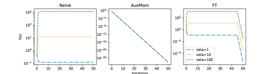
Figure 1: Effect of the bias $\zeta$ (zeta in the figure) on the naive approach (Naive), AuxMom and Fine Tuning (FT) for $K=10$,$\delta=1$ and $\eta=\min(1/2,1/(\delta K))$. We can see the naive approach fails to converge for big bias values, whereas AuxMom converges all the time no matter the value of the bias. Fine Tuning converges much slower (note the difference in scale).

Effect of the bias $\zeta$. Figure 1 shows that indeed our algorithm AuxMom does correct for the bias. We note that in this simple example, having a big value of $\zeta$ means that the gradients of $h$ point are opposite to those of $f$ and hence it’s better to not use them in a naive way. However, our approach can correct for this automatically and hence does not suffer from increasing values of $\zeta$. In real-world data, it is very difficult to quantify $\zeta$, hence why we can still benefit a little bit (in non-extreme cases) using the naive way.

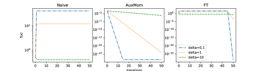
Figure 2: Effect of the similarity $\delta$ (delta in the figure) on both the naive approach (Naive), AuxMom and Fine Tuning for $K=10$,$\zeta=10$ and $\eta=\min(1/2,1/(\delta K))$. We can see the naive approach fails to benefit from small values of $\delta$, AuxMom does not suffer from the same problem, whereas Fine Tuning is slower than AuxMom.

Effect of the similarity $\delta$. Figure 2 shows how the three approaches compare when changing $\delta$. We note that $\delta=0.1$ corresponds to $L/\delta=K=10$ the value used in our experiment, our theory predicts that for values of $\delta$, the convergence is as if we were using only gradients of $f$.

6.2 Leveraging noisy or mislabeled data

We show here how our approach can be used to leverage data with questionable quality, like the case where some of the inputs might be noisy or in general transformed in a way that does not preserve the labels. A second example is when a part of the data is either unlabeled or has wrong labels.

We consider a simple feed-forward neural network ($Linear(28*28,512)\rightarrow ReLU\rightarrow Linear(512,512)\rightarrow ReLU\rightarrow Linear(512,10)$) to classify the MNIST dataset (LeCun & Cortes, 2010) which is the main task $f$. As a helper function $h$ we rotate MNIST images by a certain angle $\in\{0,45,90,180\}$. The rotation plays the role of heterogeneity. We note that this is not simple data augmentation as numbers “meanings” are not conserved under such a transformation. We plot the test accuracy that is obtained using both the naive approach and AuxMom.

First of all, Figure 3 shows that we indeed benefit from using bigger values of $K$ up to a certain level (this is predicted by our theory), this suggests that we have somehow succeeded in making a new gradient of $f$ out of each gradient of $h$ we had.

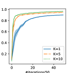
Figure 3: Effect of $K$ ($K-1$ is the number of times we use the helper h) on the test accuracy on the main task (for an angle = 45). We can see that our approach, as our theory predicts, benefits from bigger values of $K$.

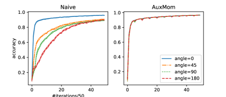
Figure 4: Test accuracy obtained using different angles as helpers, for $K=10$, step size $\eta=0.01$ and momentum parameter $a=0.1$. We see that, astonishingly, AuxMom does not suffer much from the change in the angle, whereas, as expected, the bigger the angle the worse the accuracy on the main task for the naive approach.

Next, Figure 4 shows how much the angle of rotation affects the performances of the naive approach and AuxMom. Astonishingly AuxMom seems to not suffer from increasing the value of the angle (which we should increase the bias).

Figure 5 shows a comparison with the fine-tuning approach as well.

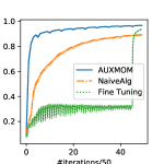
Figure 5: comparison of The Naive approach, AuxMom and Fine Tuning for an angle = 90. Again we see that while not suffering from the added bias, Fine Tuning is slower than AuxMom.

In a similar experiment, the helper $h$ is given again by MNIST images, but this time we choose a wrong label for each image with a probability $p$, Figure 6 shows the results.

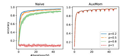
Figure 6: Test accuracy obtained using different probabilities $p$ as helpers, for $K=10$, step size $\eta=0.01$ and momentum parameter $a=0.1$. Again, astonishingly, AuxMom does not suffer much from the change in the angle, whereas, as expected, the bigger the angle the worse the accuracy on the main task.

6.3 Semi-supervised logistic regression

We consider a semi-supervised logistic regression task on the "mushrooms" dataset which has $8124$ samples each with $112$ features. We divide this dataset into three equal parts, one for training and one for testing, and the third one is unlabeled. In this context, the helper task $h$ is constituted of the unlabeled data to which random labels were assigned. Figure 7 shows indeed AuxMom accelerates convergence on the training set, more importantly, it also leads to a smaller loss on the test set which suggests a generalization benefit coming from the use of the unlabeled set.

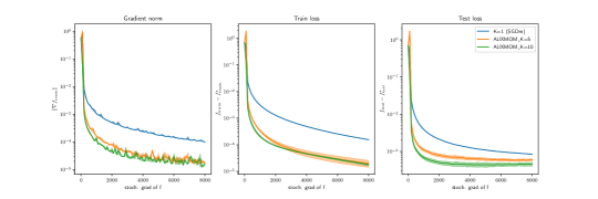
Figure 7: Gradient norm, train loss, and test loss. The parameter $a$ was chosen $a=0.1$ and the stepsizes were optimized using grid-search for best training loss.

7 Discussion

Fine Tuning. Fine Tuning uses the helper gradients first, and then uses the gradients of $f$, in this sense fine-tuning has the advantage that it can be used for different functions $f$ without having to go through the first phase each time. AuxMom seems to beat it, however, it does not enjoy the same advantage. Can we reconcile both worlds?
Better measures of similarity? Quantifying similarity between functions of the previous stochastic form is an open problem in Machine Learning that touches many domains such as Federated learning, transfer learning, curriculum learning and continual learning. Knowing what measure is most appropriate for each case is an interesting problem. In this work, we don’t pretend to solve the latter problem.
Higher order strategies. We believe our work can be “easily” extended to higher order strategies by using proxies of $f-h$ based on higher order derivatives. We expect that, in general, if we use a given Taylor approximation, we will need to make assumptions about its error. For example, if we use a 2nd order Taylor approximation, we expect we will need to bound the difference of the third derivatives of $f$ and $h$; this will be similar to the analysis of the Newton algorithm with cubic regularization(Nesterov & Polyak, 2006).
Dealing with the noise of the snapshot. In this work we propose to deal with the noise of the snapshot gradient of $f-h$ using momentum, other approaches such as using batch sizes of varying sizes with training (typically a batch size that increases as convergence is near) are possible, such an approach was used in SCSG(Lihua et al., ).
Positively correlated noise. We showed in this work that we might benefit if we could sample gradients of $h$ that are positively correlated with gradients of $f$, but we did not mention how this can be done. This is an interesting question that we intend to follow in the future.

8 Conclusion

We studied the general problem of optimizing a target function with access to a set of potentially decentralized helpers. Our framework is broad enough to recover many machine learning and optimization settings. While there are different ways of solving this problem in general, we proposed two variants AuxMom and AuxMVR that we showed improve on known optimal convergence rates. We also showed how we could go beyond the bias correction we proposed; this can be accomplished by using higher-order approximations of the difference between target and helper functions. Furthermore, we only needed the hessian similarity assumption in this work, but we think it is possible to use other similarity measures depending on the solved problem; finding such measures is outside of the scope of this work, but it might be a good future direction.

Appendix A Code

The code for our experiments is available at https://anonymous.4open.science/r/OptAuxInf-77C2/README.md.

Appendix B Basic lemmas

Lemma B.1.

$\forall{\bm{a}},{\bm{b}}\in\mathbb{R}^{d},\,c>0\>:\>\|{\bm{a}}+{\bm{b}}\|_{2}^{2}\leq(1+c)\|{\bm{a}}\|_{2}^{2}+(1+\dfrac{1}{c})\|{\bm{b}}\|_{2}^{2}\,.$

Proof.

The difference of the two quantities above is exactly $\|\sqrt{c}{\bm{a}}-\frac{1}{\sqrt{c}}{\bm{b}}\|_{2}^{2}\geq 0\,.$ ∎

Lemma B.2.

$\forall N\in\mathrm{N},\forall{\bm{a}}_{1},\ldots,{\bm{a}}_{N}\in\mathbb{R}^{d}\>:\>\|\sum_{i=1}^{N}{\bm{a}}_{i}\|_{2}^{2}\leq N\sum_{i=1}^{N}\|{\bm{a}}_{i}\|_{2}^{2}\,.$

Lemma B.3.

It is common knowledge that if $f$ is $L$-smooth, .i.e. satisfies A3.1 then :

$$\forall{\bm{x}},{\bm{y}}\in\mathbb{R}^{d}\;:f({\bm{y}})-f({\bm{x}})\leq\nabla f({\bm{x}})^{\top}({\bm{y}}-{\bm{x}})+\frac{L}{2}\|{\bm{y}}-{\bm{x}}\|_{2}^{2}\,.$$

Appendix C Missing proofs

C.1 Naive approach

As a reminder, the naive approach uses one unbiased gradient of $f$ at the beginning of each cycle followed by $K-1$ unbiased gradients of $h$.

0:  ${\bm{x}}_{0}$,${\bm{m}}^{0}$, $\eta$, $T$, $K$

  for $t=1$ to $T$ do

     Sample $\xi^{t}_{f}$; compute ${\bm{g}}_{f}({\bm{x}}^{t-1},\xi^{t}_{f})$

     ${\bm{m}}^{t}={\bm{g}}_{f}({\bm{x}}^{t-1},\xi^{t}_{f})$

     ${\bm{y}}^{t}_{0}={\bm{x}}^{t-1}$

     for $k=0$ to $K-1$ do

        if k=0 then

           ${\bm{d}}^{t}_{k}={\bm{m}}^{t}$

        else

           Sample $\xi^{t,k}_{h}$;  Compute ${\bm{g}}_{h}({\bm{y}}^{t}_{k},\xi^{t,k}_{h})$

           ${\bm{d}}^{t}_{k}={\bm{g}}_{h}({\bm{y}}^{t}_{k},\xi^{t,k}_{h})$

        end if

        ${\bm{y}}^{t}_{k+1}={\bm{y}}^{t}_{k}-\eta{\bm{d}}^{t}_{k}$

     end for

     Update ${\bm{x}}^{t}={\bm{y}}^{t}_{K}$

  end for

Algorithm 2 Naive$(f,h)$

We prove the following theorem :

Theorem C.1.

Under Assumptions 3.1,3.2,4.1. Starting from ${\bm{x}}^{0}$ and using a step size $\eta$ we have :

$$\frac{1}{2KT}\sum_{t=1}^{T}\mathbb{E}[\|\nabla f({\bm{x}}^{t-1})\|_{2}^{2}]+\frac{1-m}{2KT}\sum_{t=1}^{T}\sum_{k=2}^{K}\mathbb{E}[\|\nabla f({\bm{y}}^{t}_{k-1})\|_{2}^{2}]\leq\frac{F^{0}}{KT\eta}+\frac{L\sigma^{2}}{2}\eta+\frac{K-1}{K}\zeta^{2}\,.$$

For $\sigma^{2}=\frac{\sigma_{f}^{2}+(K-1)\sigma_{h}^{2}}{K}$ the average variance, $F^{0}=\mathbb{E}[f({\bm{x}}^{0})]-f^{\star}$.

Proof.

The proof is based on biased SGD theory. From (Ajalloeian & Stich, 2020) we have that if we the gradients ${\bm{g}}({\bm{x}})$ that we are using are such that :

$$\mathbb{E}[{\bm{g}}({\bm{x}})]=\nabla f({\bm{x}})+{\bm{b}}({\bm{x}})$$

For a target function $f$ and a gradient bias ${\bm{b}}({\bm{x}})$. Then we have for $\eta\leq\frac{1}{L}$:

$$f({\bm{y}}^{t}_{k+1})-f({\bm{y}}^{t}_{k})\leq\frac{\eta}{2}\big{(}-\|\nabla f({\bm{y}}^{t}_{k})\|_{2}^{2}+\|{\bm{b}}({\bm{y}}^{t}_{k})\|_{2}^{2}\big{)}+\frac{L\eta^{2}}{2}\sigma_{k}^{2}$$

In our case, by Assumption4.1 : $\|{\bm{b}}({\bm{y}}^{t}_{k})\|_{2}^{2}\leq\big{(}\zeta^{2}+m\|\nabla f({\bm{y}}^{t}_{k})\|_{2}^{2}\big{)}1_{k>0}$ and $\sigma_{k}^{2}=1_{k=0}\sigma_{f}^{2}+1_{k>0}\sigma_{h}^{2}$.
Summing the above inequality from $t=1,k=0$ to $t=T,k=K-1$ and then dividing by $KT$ we get the statement of the theorem. ∎

Lower bound.

It is not difficult to prove that we cannot do better using the naive strategy. We can for example pick in $1d$ a target function $f(x)=\frac{1}{2}x^{2}$ and an auxiliary function $h(x)=\frac{1}{2}(x-\zeta)^{2}$. Both functions are $1$-smooth and satisfy hessian similarity with $\delta=0$, however, $\zeta$ is not (necessarily zero), in particular, this shows that hessian similarity (Assumption3.3) and gradient dissimilarity (Assumption4.1) are orthogonal. To show the lower bound we can consider the perfect case where we have access to full gradients of $f$ and $h$.

The dynamics of the naive approach can be written in the form:

$${\bm{x}}^{t+1}=(1-\eta){\bm{x}}^{t}+\eta\zeta 1_{t\neq 0mod(K)}$$

Which implies

$${\bm{x}}^{t} =(1-\eta)^{t}{\bm{x}}^{0}+\zeta\sum_{i=0}^{t-1}\eta(1-\eta)^{t-i-1}1_{i\neq 0mod(K)}$$

$$=(1-\eta)^{t}{\bm{x}}^{0}+\Omega(\zeta)$$

This sequence does not converge to zero no matter the choice of $\eta<1$.

C.2 Momentum with auxiliary information

C.2.1 Algorithm description

The algorithm that we proposed proceeds in cycles, at the beginning of each cycle we have ${\bm{x}}^{t-1}$ and take $K$ iterations of the form ${\bm{y}}^{t}_{k}={\bm{y}}^{t}_{k-1}-\eta{\bm{d}}^{t}_{k}$ where ${\bm{y}}^{t}_{0}={\bm{x}}^{t-1}$, ${\bm{d}}^{t}_{k}={\bm{g}}_{h}({\bm{y}}^{t}_{k-1},\xi^{t}_{h,k})+{\bm{m}}^{t}$ and ${\bm{m}}^{t}=(1-a){\bm{m}}^{t-1}+a{\bm{g}}_{f-h}({\bm{x}}^{t-1},\xi^{t-1}_{f-h})$. Then we set ${\bm{x}}^{t}={\bm{y}}^{t}_{K}$.

0:  ${\bm{x}}_{0}$,${\bm{m}}^{0}$, $\eta$, $a$, $T$, $K$

  for $t=1$ to $T$ do

     Sample $\xi^{t}_{f-h}$; compute ${\bm{g}}_{f-h}({\bm{x}}^{t-1},\xi^{t}_{f-h})$

     ${\bm{m}}^{t}=(1-a){\bm{m}}^{t-1}+a{\bm{g}}_{f-h}({\bm{x}}^{t-1},\xi^{t-1}_{f-h})$

     ${\bm{y}}^{t}_{0}={\bm{x}}^{t-1}$

     for $k=0$ to $K-1$ do

        Sample $\xi^{t,k}_{h}$;  Compute ${\bm{g}}_{h}({\bm{y}}^{t}_{k},\xi^{t,k}_{h})$

        ${\bm{d}}^{t}_{k}={\bm{g}}_{h}({\bm{y}}^{t}_{k},\xi^{t,k}_{h})+{\bm{m}}^{t}$

        ${\bm{y}}^{t}_{k+1}={\bm{y}}^{t}_{k}-\eta{\bm{d}}^{t}_{k}$

     end for

     Update ${\bm{x}}^{t}={\bm{y}}^{t}_{K}$

  end for

Algorithm 3 AUXMOM$(f,h)$

We will introduce $\bar{{\bm{d}}}^{t}_{k}=\nabla h({\bm{y}}^{t}_{k-1})+{\bm{m}}^{t}$ and we note that $\mathbb{E}[{\bm{d}}^{t}_{k}|{\bm{y}}^{t}_{k-1}]=\bar{{\bm{d}}}^{t}_{k}$ and $\mathbb{E}[\|{\bm{d}}^{t}_{k}-\bar{{\bm{d}}}^{t}_{k}\|_{2}^{2}]\leq\sigma_{h}^{2}$. We will be using this fact and sometimes we will condition on ${\bm{y}}^{t}_{k-1}$ implicitly to replace ${\bm{d}}^{t}_{k}$ by $\bar{{\bm{d}}}^{t}_{k}$.

C.2.2 Convergence rate

We prove the following theorem that gives the convergence rate of this algorithm in the non-convex case.

Theorem C.2.

Under assumptions A3.1, 3.2,3.3. For $a=32\delta K\eta$ and $\eta=\min(\frac{1}{L},\frac{1}{192\delta K},\sqrt{\frac{\tilde{F}}{128L\beta KT\sigma_{f}^{2}}})\,.$ This choice gives us the rate :

$$\frac{1}{8KT}\sum_{t=1}^{T}\sum_{k=0}^{K-1}\mathbb{E}\big{[}\|\nabla f({\bm{y}}^{t}_{k})\|_{2}^{2}\big{]}\leq 24\sqrt{\frac{L\beta\tilde{F}\sigma_{f}^{2}}{T}}+\frac{(L+192\delta K)\tilde{F}}{KT}\,.$$

where $\tilde{F}=F^{0}+\frac{E^{0}}{16\delta}$, $\beta=\frac{\delta}{L}\bigg{(}\frac{\sigma_{f-h}^{2}}{\sigma_{f}^{2}}+\frac{1}{16K}\frac{\sigma_{h}^{2}}{\sigma_{f}^{2}}\bigg{)}+\frac{1}{256K}\frac{\sigma_{h}^{2}}{\sigma_{f}^{2}}$, $F^{0}=f({\bm{x}}^{0})-f^{\star}$ and $E^{0}=\mathbb{E}[\|{\bm{m}}^{0}-\nabla f({\bm{x}}^{0})+\nabla h({\bm{x}}^{0})\|_{2}^{2}]$.

Furthermore, if we use a batch-size $T$ times bigger for computing an estimate ${\bm{m}}^{0}$ of $\nabla f({\bm{x}}^{0})-\nabla h({\bm{x}}_{0})$, then by taking $a=\max(\frac{1}{T},32\delta K\eta)$ and replacing $\tilde{F}$ by $F^{0}$ in the expression of $\eta$, we get :

$$\frac{1}{8KT}\sum_{t=1}^{T}\sum_{k=0}^{K-1}\mathbb{E}\big{[}\|\nabla f({\bm{y}}^{t}_{k})\|_{2}^{2}\big{]}\leq 24\sqrt{\frac{L\beta F^{0}\sigma_{f}^{2}}{T}}+\frac{(L+192\delta K)\tilde{F}}{KT}+\frac{2\sigma_{f-h}^{2}}{T}\,.$$

C.2.3 Bias in helpers updates and Notation

Lemma C.3.

Under the $\delta$-Bounded Hessian Dissimilarity assumption, we have :
$\forall{\bm{x}},{\bm{y}}\in\mathbb{R}^{d}\;$ : $\|\nabla h({\bm{y}})-\nabla h({\bm{x}})-\nabla f({\bm{y}})+\nabla f({\bm{x}})\|^{2}\leq\delta^{2}\|{\bm{y}}-{\bm{x}}\|^{2}\,.$

Proof.

A simple application of the $\delta$-Bounded Hessian Dissimilarity assumption. ∎

Notation : We will use the following notations : ${\bm{e}}^{t}={\bm{m}}^{t}-\nabla f({\bm{x}}^{t-1})+\nabla h({\bm{x}}^{t-1})$ to denote the momentum error and $E^{t}=\mathbb{E}[\|{\bm{e}}^{t}\|_{2}^{2}]$ to denote its expected squared norm. $\Delta^{t}_{k}=\mathbb{E}[\|{\bm{y}}^{t}_{k}-{\bm{x}}^{t-1}\|^{2}]$ will denote the progress made up to the k-th round of the t-th cycle, and for the progress in a whole cycle we will use $\Delta^{t}=\mathbb{E}[\|{\bm{x}}^{t}-{\bm{x}}^{t-1}\|^{2}]$. We also denote $\bar{{\bm{d}}}^{t}_{k}={\bm{d}}^{t}_{k}-{\bm{g}}_{h}({\bm{y}}^{t}_{k},\xi^{t,k}_{h})+\nabla h({\bm{y}}^{t}_{k-1})=\nabla h({\bm{y}}^{t}_{k-1})+{\bm{m}}^{t}.$

C.2.4 Change during each cycle

Variance of $\bar{{\bm{d}}}^{t}_{k}$. We would like $\bar{{\bm{d}}}^{t}_{k}$ to be $\nabla f({\bm{y}}^{t}_{k-1})$, but it is not. In the next lemma, we control the error resulting from these two quantities being different.

Lemma C.4.

Under assumption A3.3, we have the following inequality :

$$\mathbb{E}[\|\bar{{\bm{d}}}^{t}_{k}-\nabla f({\bm{y}}^{t}_{k-1})\|_{2}^{2}]\leq 2\delta^{2}\Delta^{t}_{k-1}+2E^{t}$$

Proof.

We have

$$\bar{{\bm{d}}}^{t}_{k}-\nabla f({\bm{y}}^{t}_{k-1}) =\nabla h({\bm{y}}^{t}_{k-1})-\nabla f({\bm{y}}^{t}_{k-1})+{\bm{m}}^{t}$$

$$=h({\bm{y}}^{t}_{k-1})-\nabla f({\bm{y}}^{t}_{k-1})-\nabla f({\bm{y}}^{t}_{k-1})+\nabla f({\bm{x}}^{t-1})+{\bm{m}}^{t}-\nabla f({\bm{x}}^{t-1})+\nabla h({\bm{x}}^{t-1})$$

$$=h({\bm{y}}^{t}_{k-1})-\nabla f({\bm{y}}^{t}_{k-1})-\nabla f({\bm{y}}^{t}_{k-1})+\nabla f({\bm{x}}^{t-1})+{\bm{e}}^{t}$$

Using Lemma B.1 with $c=1$, we get :

$$\mathbb{E}[\|\bar{{\bm{d}}}^{t}_{k}-\nabla f({\bm{y}}^{t}_{k-1})\|_{2}^{2}] \leq 2\mathbb{E}[\|h({\bm{y}}^{t}_{k-1})-\nabla f({\bm{y}}^{t}_{k-1})-\nabla f({\bm{y}}^{t}_{k-1})+\nabla f({\bm{x}}^{t-1})\|_{2}^{2}]+2\mathbb{E}[\|{\bm{e}}^{t}\|_{2}^{2}]$$

$$\leq 2\delta^{2}\|{\bm{y}}^{t}_{k-1}-{\bm{x}}^{t-1}\|_{2}^{2}+2\mathbb{E}[\|{\bm{e}}^{t}\|_{2}^{2}]$$

$$=2\delta^{2}\Delta^{t}_{k-1}+2E^{t}$$

∎

Distance moved in each step.

Lemma C.5.

for $\eta\leq\frac{1}{5\delta K}$ we have:

$$\Delta^{t}_{k}\leq(1+\frac{1}{K})\Delta^{t}_{k-1}+12K\eta^{2}E^{t}+6K\eta^{2}\mathbb{E}[\|\nabla f({\bm{y}}^{t}_{k-1})\|_{2}^{2}]+\eta^{2}\sigma_{h}^{2}\,.$$

Proof.

$$\Delta^{t}_{k} =\mathbb{E}[\|{\bm{y}}^{t}_{k}-{\bm{x}}^{t-1}\|_{2}^{2}]$$

$$=\mathbb{E}[\|{\bm{y}}^{t}_{k-1}-\eta{\bm{d}}^{t}_{k}-{\bm{x}}^{t-1}\|_{2}^{2}]$$

$$=\mathbb{E}[\|{\bm{y}}^{t}_{k-1}-\eta\bar{{\bm{d}}}^{t}_{k}-{\bm{x}}^{t-1}\|_{2}^{2}]+\eta^{2}\mathbb{E}[\|{\bm{d}}^{t}_{k}-\bar{{\bm{d}}}^{t}_{k}\|_{2}^{2}]$$

$$\leq(1+\frac{1}{2K})\Delta^{t}_{k-1}+(2K+1)\eta^{2}\mathbb{E}[\|\bar{{\bm{d}}}^{t}_{k}\|_{2}^{2}]+\eta^{2}\sigma_{h}^{2}$$

$$=(1+\frac{1}{2K})\Delta^{t}_{k-1}+3K\eta^{2}\mathbb{E}[\|\bar{{\bm{d}}}^{t}_{k}\pm\nabla f({\bm{y}}^{t}_{k-1})\|_{2}^{2}]+\eta^{2}\sigma_{h}^{2}$$

$$\leq(1+\frac{1}{2K})\Delta^{t}_{k-1}+6K\eta^{2}\mathbb{E}[\|\bar{{\bm{d}}}^{t}_{k}-\nabla f({\bm{y}}^{t}_{k-1})\|_{2}^{2}]+6K\eta^{2}\mathbb{E}[\|\nabla f({\bm{y}}^{t}_{k-1})\|_{2}^{2}]+\eta^{2}\sigma_{h}^{2}$$

$$\leq(1+\frac{1}{2K})\Delta^{t}_{k-1}+6K\eta^{2}(2\delta^{2}\Delta^{t}_{k-1}+2E^{t})+6K\eta^{2}\mathbb{E}[\|\nabla f({\bm{y}}^{t}_{k-1})\|_{2}^{2}]+\eta^{2}\sigma_{h}^{2}$$

$$=(1+\frac{1}{2K}+12\delta^{2}K\eta^{2})\Delta^{t}_{k-1}+12K\eta^{2}E^{t}+6K\eta^{2}\mathbb{E}[\|\nabla f({\bm{y}}^{t}_{k-1})\|_{2}^{2}]+\eta^{2}\sigma_{h}^{2}$$

The condition $\eta\leq\frac{1}{5\delta K}$ ensures $12\delta^{2}K\eta^{2}\leq\frac{1}{2K}$ which finishes the proof.

∎

Progress in one step.

Lemma C.6.

For $\eta\leq\min(\frac{1}{L},\frac{1}{192\delta K})$, under assumptions A3.1 and A3.3, the following inequality is true:

$$\mathbb{E}\big{[}f({\bm{y}}^{t}_{k})+\delta(1+\frac{2}{K})^{K-k}\Delta^{t}_{k}\big{]} \leq\mathbb{E}\big{[}f({\bm{y}}^{t}_{k-1})+\delta(1+\frac{2}{K})^{K-(k-1)}\Delta^{t}_{k-1}\big{]}$$

$$-\frac{\eta}{4}\mathbb{E}[\|\nabla f({\bm{y}}^{t}_{k-1})\|_{2}^{2}]+2\eta E^{t}+(\frac{L}{2}+8\delta)\eta^{2}\sigma_{h}^{2}\,.$$

Proof.

The $L$-smoothness of $f$ guarantees :

$$f({\bm{y}}^{t}_{k})-f({\bm{y}}^{t}_{k-1})\leq-\eta\nabla f({\bm{y}}^{t}_{k-1})^{\top}{\bm{d}}^{t}_{k}+\frac{L\eta^{2}}{2}\|{\bm{d}}^{t}_{k}\|_{2}^{2}\,.$$

By taking expectation conditional to the knowledge of ${\bm{y}}^{t}_{k-1}$ we have:

$$\mathbb{E}[f({\bm{y}}^{t}_{k})-f({\bm{y}}^{t}_{k-1})]\leq-\eta\mathbb{E}[\nabla f({\bm{y}}^{t}_{k-1})^{\top}\bar{{\bm{d}}}^{t}_{k}]+\frac{L\eta^{2}}{2}\mathbb{E}[\|\bar{{\bm{d}}}^{t}_{k}\|_{2}^{2}]+\frac{L\eta^{2}}{2}\sigma_{h}^{2}\,.$$

Using the identity $-2ab=(a-b)^{2}-a^{2}-b^{2}$, we have :

$$E[f({\bm{y}}^{t}_{k})-f({\bm{y}}^{t}_{k-1})]\leq-\frac{\eta}{2}E[\|\nabla f({\bm{y}}^{t}_{k-1})\|_{2}^{2}]+\frac{\eta}{2}E[\|{\bm{d}}^{t}_{k}-\nabla f({\bm{y}}^{t}_{k-1})\|_{2}^{2}]+\frac{L\eta^{2}-\eta}{2}E[\|{\bm{d}}^{t}_{k}\|_{2}^{2}]+\frac{L\eta^{2}}{2}\sigma_{h}^{2}\,.$$

Using $\eta\leq\frac{1}{L}$ we can get rid of the last term in the above inequality.

Using LemmaC.4, we get :

$$\mathbb{E}[f({\bm{y}}^{t}_{k})-f({\bm{y}}^{t}_{k-1})] \leq-\frac{\eta}{2}\mathbb{E}\big{[}\|\nabla f({\bm{y}}^{t}_{k-1})\|_{2}^{2}\big{]}+\frac{\eta}{2}\mathbb{E}\big{[}\|{\bm{d}}^{t}_{k}-\nabla f({\bm{y}}^{t}_{k-1})\|_{2}^{2}\big{]}+\frac{L\eta^{2}}{2}\sigma_{h}^{2}$$

$$\leq-\frac{\eta}{2}\mathbb{E}\big{[}\|\nabla f({\bm{y}}^{t}_{k-1})\|_{2}^{2}\big{]}+\frac{\eta}{2}(2\delta^{2}\Delta^{t}_{k-1}+2E^{t})+\frac{L\eta^{2}}{2}\sigma_{h}^{2}$$

$$=\delta^{2}\eta\Delta^{t}_{k-1}+\eta E^{t}-\frac{\eta}{2}\mathbb{E}\big{[}\|\nabla f({\bm{y}}^{t}_{k-1})\|_{2}^{2}\big{]}+\frac{L\eta^{2}}{2}\sigma_{h}^{2}\,.$$

Now we multiply LemmaC.5 by $\delta(1+\frac{2}{K})^{K-k}$. Note that $1\leq(1+\frac{2}{K})^{K-k}\leq 8$.

$$\delta(1+\frac{2}{K})^{K-k}\Delta^{t}_{k} \leq\delta(1+\frac{2}{K})^{K-k}\big{(}(1+\frac{1}{K})\Delta^{t}_{k-1}+12K\eta^{2}E^{t}+6K\eta^{2}\mathbb{E}[\|\nabla f({\bm{y}}^{t}_{k-1})\|_{2}^{2}]\big{)}$$

$$+\delta(1+\frac{2}{K})^{K-k}\eta^{2}\sigma_{h}^{2}$$

$$\leq\delta(1+\frac{2}{K})^{K-(k-1)}\Delta^{t}_{k-1}-\frac{\delta}{K}(1+\frac{2}{K})^{K-k}\Delta^{t}_{k-1}+96K\delta\eta^{2}E^{t}$$

$$+48K\delta\eta^{2}\mathbb{E}[\|\nabla f({\bm{y}}^{t}_{k-1})\|_{2}^{2}]+8\delta\eta^{2}\sigma_{h}^{2}$$

$$\leq\delta(1+\frac{2}{K})^{K-(k-1)}\Delta^{t}_{k-1}-\frac{\delta}{K}\Delta^{t}_{k-1}+96K\delta\eta^{2}E^{t}$$

$$+48K\delta\eta^{2}\mathbb{E}[\|\nabla f({\bm{y}}^{t}_{k-1})\|_{2}^{2}]+8\delta\eta^{2}\sigma_{h}^{2}$$

Adding the last two inequalities, we get :

$$\mathbb{E}[f({\bm{y}}^{t}_{k})]+\delta(1+\frac{2}{K})^{K-k}\Delta^{t}_{k} \leq\mathbb{E}[f({\bm{y}}^{t}_{k-1})]+\delta(1+\frac{2}{K})^{K-(k-1)}\Delta^{t}_{k-1}$$

$$+(\delta^{2}\eta-\frac{\delta}{K})\Delta^{t}_{k-1}$$

$$+(\eta+96K\delta\eta^{2})E^{t}$$

$$+(-\frac{\eta}{2}+48K\delta\eta^{2})\mathbb{E}[\|\nabla f({\bm{y}}^{t}_{k-1})\|_{2}^{2}]$$

$$+(L/2+8\delta)\eta^{2}\sigma_{h}^{2}$$

For $\eta\leq\frac{1}{192\delta K}$ we have $\delta^{2}\eta-\frac{\delta}{K}\leq 0$, $\eta+96K\delta\eta^{2}\leq 2\eta$ and $-\frac{\eta}{2}+48K\delta\eta^{2}\leq-\frac{\eta}{4}$ which gives the lemma. ∎

Distance moved in a cycle.

Lemma C.7.

For $\eta\leq\frac{1}{5K\delta}$ and under assumptions A3.1 and A3.3 with $G^{t}=\frac{1}{K}\sum_{k=0}^{K-1}\mathbb{E}\big{[}\|\nabla f({\bm{y}}^{t}_{k})\|_{2}^{2}\big{]}$, we have :

$$\Delta^{t}\Big{(}:=\mathbb{E}\big{[}\|{\bm{x}}^{t}-{\bm{x}}^{t-1}\|_{2}^{2}\big{]}\Big{)}\leq 36K^{2}\eta^{2}E^{t}+18K^{2}\eta^{2}G^{t}+3K\eta^{2}\sigma_{h}^{2}\,.$$

Proof.

We use the fact ${\bm{x}}^{t}={\bm{y}}^{t}_{K}$, which means $\Delta^{t}=\Delta^{t}_{K}$. The recurrence established in LemmaC.5 implies :

$$\Delta^{t} \leq\sum_{k=1}^{K}(1+\frac{1}{K})^{K-k}\Big{(}12K\eta^{2}E^{t}+6K\eta^{2}\mathbb{E}[\|\nabla f({\bm{y}}^{t}_{k-1})\|_{2}^{2}]+\eta^{2}\sigma_{h}^{2}\Big{)}$$

$$\leq 36K^{2}\eta^{2}E^{t}+18K(K+1)\eta^{2}\frac{1}{K}\sum_{k}\mathbb{E}\big{[}\|\nabla f({\bm{y}}^{t}_{k})\|_{2}^{2}\big{]}+3K\eta^{2}\sigma_{h}^{2}$$

$$=36K^{2}\eta^{2}E^{t}+18K^{2}\eta^{2}G^{t}+3K\eta^{2}\sigma_{h}^{2}\,.$$

Where we used the fact that $(1+\frac{1}{K})^{K-k}\leq 3$. ∎

Momentum variance. Here we will bound the quantity $E^{t}$.

Lemma C.8.

Under assumptions A3.1,A3.2 and for $a\geq 12K\delta\eta$ , we have :

$$E^{t}\leq(1-\frac{a}{2})E^{t-1}+\frac{32\delta^{2}K^{2}\eta^{2}}{a}G^{t-1}+a^{2}\sigma_{f-h}^{2}\,.$$

Proof.

$$E^{t} =\mathbb{E}\big{[}\|{\bm{m}}^{t}-\nabla f({\bm{x}}^{t-1})+\nabla h({\bm{x}}^{t-1})\|_{2}^{2}\big{]}$$

$$=\mathbb{E}\big{[}\|(1-a)({\bm{m}}^{t-1}-\nabla f({\bm{x}}^{t-1})+\nabla h({\bm{x}}^{t-1}))+a({\bm{g}}_{f}({\bm{x}}^{t-1})+{\bm{g}}_{h}({\bm{x}}^{t-1})-\nabla f({\bm{x}}^{t-1})+\nabla h({\bm{x}}^{t-1}))\|_{2}^{2}\big{]}$$

$$\leq(1-a)^{2}\mathbb{E}\big{[}\|{\bm{m}}^{t-1}\pm(\nabla f({\bm{x}}^{t-2})-\nabla h({\bm{x}}^{t-2}))-(\nabla f({\bm{x}}^{t-1})-\nabla f({\bm{x}}^{t-1}))\|_{2}^{2}\big{]}+a^{2}\sigma_{f-h}^{2}$$

$$\leq(1-a)^{2}(1+a/2)E^{t-1}+(1-a)^{2}(1+2/a)\mathbb{E}\big{[}\|\nabla f({\bm{x}}^{t-2})-\nabla h({\bm{x}}^{t-2})-\nabla f({\bm{x}}^{t-1})+\nabla h({\bm{x}}^{t-1})\|_{2}^{2}\big{]}$$

$$+a^{2}\sigma_{f-h}^{2}$$

$$\leq(1-a)E^{t-1}+\frac{2\delta^{2}}{a}\Delta^{t-1}+a^{2}\sigma_{f-h}^{2}$$

Where we used the L-smoothness of $f$ to get the last inequality. We have also used the inequalities $(1-a)^{2}(1+a/2)\leq(1-a)$ and $(1-a)^{2}(1+2/a)\leq 2/a$ true for all $a\in(0,1]$.

We can now use LemmaC.7 to have :

$$E^{t}\leq(1-a+\frac{72\delta^{2}K^{2}\eta^{2}}{a})E^{t-1}+\frac{32\delta^{2}K^{2}\eta^{2}}{a}G^{t-1}+a^{2}\sigma_{f-h}^{2}$$

By taking $a\geq 12\delta K\eta$ we ensure $\frac{72\delta^{2}K^{2}\eta^{2}}{a}\leq\frac{a}{2}$, So :

$$E^{t}\leq(1-\frac{a}{2})E^{t-1}+\frac{32\delta^{2}K^{2}\eta^{2}}{a}G^{t-1}+a^{2}\sigma_{f-h}^{2}$$

∎

Progress in one round.

Lemma C.9.

Under the same assumptions as in LemmaC.6, we have :

$$\frac{\eta}{4}G^{t}\leq\frac{F^{t-1}-F^{t}}{K}-\frac{\delta}{K}\Delta^{t}+2\eta E^{t}+(\frac{L}{2}+8\delta)\eta^{2}\sigma_{h}^{2}\,.$$

Where $F^{t}=\mathbb{E}[f({\bm{x}}^{t})]-f^{\star}$.

Proof.

We use the inequality established in LemmaC.6, which can be rearranged in the following way :

$$\frac{\eta}{4}\mathbb{E}[\|\nabla f({\bm{y}}^{t}_{k-1})\|_{2}] \leq\mathbb{E}\big{[}f({\bm{y}}^{t}_{k-1})+\delta(1+\frac{2}{K})^{K-(k-1)}\Delta^{t}_{k-1}\big{]}-\Big{(}\mathbb{E}\big{[}f({\bm{y}}^{t}_{k})+\delta(1+\frac{2}{K})^{K-k}\Delta^{t}_{k}\big{]}\Big{)}$$

$$+2\eta E^{t}+(\frac{L}{2}+8\delta)\eta^{2}\sigma_{h}^{2}\,.$$

We sum this inequality from $k=1$ to $k=K$, this will give:

$$\frac{K\eta}{4}G^{t}\leq\mathbb{E}\big{[}f({\bm{y}}^{t}_{0})+\delta(1+\frac{2}{K})^{K}\Delta^{t}_{0}\big{]}-\Big{(}\mathbb{E}\big{[}f({\bm{y}}^{t}_{K})+\delta\Delta^{t}_{K}\big{]}\Big{)}+2\eta KE^{t}+(\frac{L}{2}+8\delta)K\eta^{2}\sigma_{h}^{2}\,.$$

We note that ${\bm{y}}^{t}_{0}={\bm{x}}^{t-1}$ and ${\bm{y}}^{t}_{K}={\bm{x}}^{t}$, which means $\Delta^{t}_{0}=0$ and $\Delta^{t}_{K}=\Delta^{t}$. So we have :

$$\frac{\eta}{4}G^{t}\leq\frac{F^{t-1}-F^{t}}{K}-\frac{\delta}{K}\Delta^{t}+2\eta E^{t}+(\frac{L}{2}+8\delta)\eta^{2}\sigma_{h}^{2}\,.$$

∎

Let’s derive now the convergence rate.

We have :

$$\left\{\begin{array}[]{ll}\frac{\eta}{4}G^{t}\leq\frac{F^{t-1}-F^{t}}{K}+2\eta E^{t}+(\frac{L}{2}+8\delta)\eta^{2}\sigma_{h}^{2}\,,\\ E^{t}\leq(1-\frac{a}{2})E^{t-1}+\frac{32\delta^{2}K^{2}\eta^{2}}{a}G^{t-1}+a^{2}\sigma_{f-h}^{2}\,.\end{array}\right.$$

We will add to both sides of the first inequality the quantity $\frac{4\eta}{a}E^{t}$.

So :

$$\frac{\eta}{4}G^{t}+\frac{4\eta}{a}E^{t}\leq\frac{F^{t-1}-F^{t}}{K}+2\eta E^{t}+(\frac{L}{2}+8\delta)\eta^{2}\sigma_{h}^{2}+\frac{4\eta}{a}\Big{(}(1-\frac{a}{2})E^{t-1}+\frac{32\delta^{2}K^{2}\eta^{2}}{a}G^{t-1}+a^{2}\sigma_{f-h}^{2}\Big{)}\,,$$

Which gives for $a\geq 32\delta K\eta$ :

$$\frac{\eta}{4}G^{t}-\frac{\eta}{8}G^{t-1}\leq\Phi^{t-1}-\Phi^{t}+4\eta a\sigma_{f-h}^{2}+(\frac{L}{2}+8\delta)\eta^{2}\sigma_{h}^{2}\,,$$ (7)

For a potential $\Phi^{t}=\frac{F^{t}}{K}+(\frac{4\eta}{a}-2\eta)E^{t}\leq\frac{F^{t}}{K}+\frac{2\eta}{a}E^{t}$.

Summing the inequality 7 over $t$, gives :

$$\frac{1}{8T}\sum_{t=1}^{T}G^{t} \leq\frac{\Phi^{0}}{\eta T}+4a(\sigma_{f}^{2}+\sigma_{h}^{2})+(\frac{L}{2}+8\delta)\eta\sigma_{h}^{2}\,,$$

$$\leq\frac{F^{0}}{\eta KT}+\frac{2}{aT}E^{0}+4a\sigma_{f-h}^{2}+(\frac{L}{2}+8\delta)\eta\sigma_{h}^{2}\,,$$

Now taking $$a=32\delta K\eta\leq 1$$, we get :

$$\frac{1}{8T}\sum_{t=1}^{T}G^{t} \leq\frac{F^{0}}{\eta KT}+\frac{1}{16\delta K\eta T}E^{0}+128\delta K\eta\sigma_{f-h}^{2}+(\frac{L}{2}+8\delta)\eta\sigma_{h}^{2}\,,$$

$$=\frac{\tilde{F}}{\eta KT}+128\delta K\eta\sigma_{f-h}^{2}+(\frac{L}{2}+8\delta)\eta\sigma_{h}^{2}\,,$$

$$=\frac{\tilde{F}}{\eta KT}+128L\beta K\eta\sigma_{f}^{2}\,,$$

For $$\tilde{F}=F^{0}+\frac{E^{0}}{16\delta} \beta=\frac{\delta}{L}\bigg{(}\frac{\sigma_{f-h}^{2}}{\sigma_{f}^{2}}+\frac{1}{16K}\frac{\sigma_{h}^{2}}{\sigma_{f}^{2}}\bigg{)}+\frac{1}{256K}\frac{\sigma_{h}^{2}}{\sigma_{f}^{2}}$$ and .

Taking into account all the conditions on $\eta$ that were necessary, we can take :

$$\eta=\min(\frac{1}{L},\frac{1}{192\delta K},\sqrt{\frac{\tilde{F}}{128L\beta K^{2}T\sigma_{f}^{2}}})\,.$$

This choice gives us the rate :

$$\frac{1}{8T}\sum_{t=1}^{T}G^{t}\leq 24\sqrt{\frac{L\beta\tilde{F}\sigma_{f}^{2}}{T}}+\frac{(L+192\delta K)\tilde{F}}{KT}\,.$$

As for dealing with $E^{0}$ if we use a batch-size $S$ times bigger than the other batch-sizes we have $E^{0}\leq\frac{\sigma_{f-h}^{2}}{S}$. In particular, for $S=T$, $E^{0}\leq\frac{\sigma_{f-h}^{2}}{S}$, this way we get $\tilde{F}=F^{0}+\frac{\sigma_{f-h}^{2}}{16\delta T}$.

We can also take $a=\max(\frac{1}{T},32\delta K\eta)$, we get :

$$\frac{1}{8T}\sum_{t=1}^{T}G^{t}\leq 24\sqrt{\frac{L\beta F^{0}\sigma_{f}^{2}}{T}}+\frac{(L+192\delta K)\tilde{F}}{KT}+\frac{2\sigma_{f-h}^{2}}{T}\,.$$

C.3 MVR with auxiliary information

C.3.1 Algorithm description

The algorithm that we proposed proceeds in cycles, at the beginning of each cycle we have states ${\bm{x}}^{t-2}$ and ${\bm{x}}^{t-1}$. To update these states, we take $K+1$ iterations of the form ${\bm{y}}^{t}_{k}={\bm{y}}^{t}_{k-1}-\eta{\bm{d}}^{t}_{k}$ where ${\bm{y}}^{t}_{0}={\bm{x}}^{t-1}$, ${\bm{d}}^{t}_{k}={\bm{g}}_{h}({\bm{y}}^{t}_{k-1},\xi^{t}_{h,k})+(1-a){\bm{m}}^{t-1}+a{\bm{g}}_{f-h}({\bm{x}}^{t-2},\xi^{t-1}_{f-h})$ and ${\bm{m}}^{t}=(1-a){\bm{m}}^{t-1}+a{\bm{g}}_{f-h}({\bm{x}}^{t-1},\xi^{t-1}_{f-h})+(1-a)\Big{(}{\bm{g}}_{f-h}({\bm{x}}^{t-1},\xi^{t-1}_{f-h})-{\bm{g}}_{f-h}({\bm{x}}^{t-2},\xi^{t-1}_{f-h}))$. Then we set ${\bm{x}}^{t}={\bm{y}}^{t}_{K}$.

0:  ${\bm{x}}_{0}$,${\bm{m}}^{0}$, $\eta$, $a$, $T$, $K$

  ${\bm{x}}_{-1}={\bm{x}}_{0}$

  for $t=1$ to $T$ do

     Sample $\xi^{t}_{f-h}$

     ${\bm{g}}^{f-h}_{prev}={\bm{g}}_{f-h}({\bm{x}}^{t-2},\xi^{t}_{f-h})$

     ${\bm{g}}^{f-h}={\bm{g}}_{f-h}({\bm{x}}^{t-1},\xi^{t}_{f-h})$

     ${\bm{y}}^{t}_{0}={\bm{x}}^{t-1}$

     for $k=0$ to $K-1$ do

        Sample $\xi^{t,k}_{h}$;  Compute ${\bm{g}}_{h}({\bm{y}}^{t}_{k},\xi^{t,k}_{h})$

        ${\bm{d}}^{t}_{k}={\bm{g}}_{h}({\bm{y}}^{t}_{k},\xi^{t,k}_{h})+(1-a){\bm{m}}^{t-1}+a{\bm{g}}^{f-h}_{prev}$

        ${\bm{y}}^{t}_{k+1}={\bm{y}}^{t}_{k}-\eta{\bm{d}}^{t}_{k}$

     end for

     ${\bm{m}}^{t}=(1-a){\bm{m}}^{t-1}+a{\bm{g}}^{f-h}+(1-a)({\bm{g}}^{f-h}-{\bm{g}}^{f-h}_{prev})$ §update momentum

     Update ${\bm{x}}^{t}={\bm{y}}^{t}_{K}$

  end for

Algorithm 4 AUXMVR$(f,h)$

Notation change. From now on, we will denote $\Delta^{t}_{k}=\mathbb{E}\big{[}\|{\bm{y}}^{t}_{k}-{\bm{x}}^{t-2}\|_{2}^{2}\big{]}$, we will keep other quantities same as before. This time also we will denote $\bar{{\bm{d}}}^{t}_{k}=\nabla h({\bm{y}}^{t}_{k-1})+(1-a){\bm{m}}^{t-1}+a{\bm{g}}_{f-h}({\bm{x}}^{t-2},\xi^{t-1}_{f})$ and we note that by fixing ${\bm{y}}^{t}_{k-1}$ we have $\mathbb{E}[{\bm{d}}^{t}_{k}]=\bar{{\bm{d}}}^{t}_{k}$ and $\mathbb{E}[\|{\bm{d}}^{t}_{k}-\bar{{\bm{d}}}^{t}_{k}\|_{2}^{2}]\leq\sigma_{h}^{2}$.

C.3.2 Convergence of MVR with auxiliary information

We prove the following theorem that gives the convergence rate of this algorithm in the non-convex case.

Theorem C.10.

Under assumptions A3.1, 3.2,4.2. For $a=\max(\frac{1}{T},1296\delta^{2}K^{2}\eta^{2})$ if $\sigma_{h}=0$, $a=\max(\frac{1}{T},36\delta K\eta)$ otherwise, and $\eta=\min\bigg{(}\frac{1}{L},\frac{1}{1926\delta K},\frac{1}{K}\big{(}\frac{F^{0}}{7776\delta^{2}T\sigma_{f-h}^{2}}\big{)}^{1/3},\frac{1}{K}\sqrt{\frac{2F^{0}}{\gamma LT\sigma_{h}^{2}}}\bigg{)}\,.$ This choice gives us the rate :

$$\frac{1}{8KT}\sum_{t=1}^{T}\sum_{k=1}^{K-1}\mathbb{E}\big{[}\|\nabla f({\bm{y}}^{t}_{k})\|_{2}^{2}\big{]}\leq 2\sqrt{\frac{L\gamma F^{0}\sigma_{h}^{2}}{KT}}+30\big{(}\frac{\delta F^{0}\sigma_{f-h}}{T}\big{)}^{2/3}+\frac{(L+1926\delta K)F^{0}}{T}+\frac{3\sigma_{f-h}^{2}}{T}\,.$$

Where $F^{0}=f({\bm{x}}^{0})-f^{\star}$ and $\gamma=\frac{1}{2K}+\frac{126\delta}{L}$.

C.3.3 Change during each cycle

Variance of ${\bm{d}}^{t}_{k}$. Again ${\bm{d}}^{t}_{k}$ is not perfectly equal to $\nabla f({\bm{y}}^{t}_{k-1})$ due to the use of $h$ instead of $f$ the function we are actually optimizing. In the following lemma, we quantify the error resulting from this.

Lemma C.11.

Under assumption A3.3, we have the following inequality :

$$\mathbb{E}[\|\bar{{\bm{d}}}^{t}_{k}-\nabla f({\bm{y}}^{t}_{k-1})\|_{2}^{2}]\leq 3\delta^{2}\Delta^{t}_{k-1}+3E^{t-1}+3a^{2}\sigma_{f-h}^{2}\,.$$

Proof.

We have

$$\bar{{\bm{d}}}^{t}_{k}-\nabla f({\bm{y}}^{t}_{k-1}) =\nabla h({\bm{y}}^{t}_{k-1})+(1-a){\bm{m}}^{t-1}+a({\bm{g}}_{f}({\bm{x}}^{t-2},\xi^{t-1}_{f})-{\bm{g}}_{h}({\bm{x}}^{t-2},\xi^{t-1}_{h}))-\nabla f({\bm{y}}^{t}_{k-1})$$

$$=(1-a){\bm{e}}^{t-1}+(1-a)(\nabla f({\bm{x}}^{t-2})-\nabla h({\bm{x}}^{t-2}))$$

$$+\nabla h({\bm{y}}^{t}_{k-1})+a({\bm{g}}_{f}({\bm{x}}^{t-2},\xi^{t-1}_{f})-{\bm{g}}_{h}({\bm{x}}^{t-2},\xi^{t-1}_{h}))-\nabla f({\bm{y}}^{t}_{k-1})$$

$$=(1-a){\bm{e}}^{t-1}+a\big{(}{\bm{g}}_{f}({\bm{x}}^{t-2},\xi^{t-1}_{f})-{\bm{g}}_{h}({\bm{x}}^{t-2},\xi^{t-1}_{h})-\nabla f({\bm{x}}^{t-2})+\nabla h({\bm{x}}^{t-2})\big{)}$$

$$+\nabla h({\bm{y}}^{t}_{k-1})-\nabla h({\bm{x}}^{t-2})-\nabla f({\bm{y}}^{t}_{k-1})+\nabla f({\bm{x}}^{t-2})$$

Using Lemma B.2 with $N=3$, we get :

$$\mathbb{E}[\|{\bm{d}}^{t}_{k}-\nabla f({\bm{y}}^{t}_{k-1})\|_{2}^{2}] \leq 3\mathbb{E}[\|\nabla h({\bm{y}}^{t}_{k-1})-\nabla h({\bm{x}}^{t-2})-\nabla f({\bm{y}}^{t}_{k-1})+\nabla f({\bm{x}}^{t-2})\|_{2}^{2}]$$

$$+3(1-a)^{2}\mathbb{E}[\|{\bm{e}}^{t-1}\|_{2}^{2}]$$

$$+3a^{2}\mathbb{E}[\|{\bm{g}}_{f}({\bm{x}}^{t-2},\xi^{t-1}_{f})-{\bm{g}}_{h}({\bm{x}}^{t-2},\xi^{t-1}_{h})-\nabla f({\bm{x}}^{t-2})+\nabla h({\bm{x}}^{t-2})\|_{2}^{2}]$$

$$\leq 3\delta^{2}\Delta^{t}_{k-1}+3E^{t-1}+3a^{2}\sigma_{f-h}^{2}\,.$$

∎

Distance moved in each step.

Lemma C.12.

for $\eta\leq\frac{1}{6\delta K}$ we have:

$$\Delta^{t}_{k}\leq(1+\frac{1}{K})\Delta^{t}_{k-1}+18K\eta^{2}E^{t-1}+18K\eta^{2}a^{2}\sigma_{f-h}^{2}+6K\eta^{2}\mathbb{E}[\|\nabla f({\bm{y}}^{t}_{k-1})\|_{2}^{2}]+\eta^{2}\sigma_{h}^{2}$$

Proof.

Like for the proof of LemmaC.5, we get :

$$\Delta^{t}_{k} =\mathbb{E}[\|{\bm{y}}^{t}_{k}-{\bm{x}}^{t-2}\|_{2}^{2}]$$

$$=\mathbb{E}[\|{\bm{y}}^{t}_{k-1}-\eta{\bm{d}}^{t}_{k}-{\bm{x}}^{t-2}\|_{2}^{2}]$$

$$=\mathbb{E}[\|{\bm{y}}^{t}_{k-1}-\eta\bar{{\bm{d}}}^{t}_{k}-{\bm{x}}^{t-2}\|_{2}^{2}]+\eta^{2}\mathbb{E}[\|{\bm{d}}^{t}_{k}-\bar{{\bm{d}}}^{t}_{k}\|_{2}^{2}]$$

$$\leq(1+\frac{1}{2K})\Delta^{t}_{k-1}+(2K+1)\eta^{2}\mathbb{E}[\|\bar{{\bm{d}}}^{t}_{k}\|_{2}^{2}]+\eta^{2}\sigma_{h}^{2}$$

$$=(1+\frac{1}{2K})\Delta^{t}_{k-1}+3K\eta^{2}\mathbb{E}[\|{\bm{d}}^{t}_{k}\pm\nabla f({\bm{y}}^{t}_{k-1})\|_{2}^{2}]+\eta^{2}\sigma_{h}^{2}$$

$$\leq(1+\frac{1}{2K})\Delta^{t}_{k-1}+6K\eta^{2}\mathbb{E}[\|\bar{{\bm{d}}}^{t}_{k}-\nabla f({\bm{y}}^{t}_{k-1})\|_{2}^{2}]+6K\eta^{2}\mathbb{E}[\|\nabla f({\bm{y}}^{t}_{k-1})\|_{2}^{2}]+\eta^{2}\sigma_{h}^{2}$$

$$\leq(1+\frac{1}{2K})\Delta^{t}_{k-1}+6K\eta^{2}(3\delta^{2}\Delta^{t}_{k-1}+3E^{t-1}+3a^{2}\sigma_{f-h}^{2})+6K\eta^{2}\mathbb{E}[\|\nabla f({\bm{y}}^{t}_{k-1})\|_{2}^{2}]+\eta^{2}\sigma_{h}^{2}$$

$$=(1+\frac{1}{2K}+18\delta^{2}K\eta^{2})\Delta^{t}_{k-1}+18K\eta^{2}E^{t}+18K\eta^{2}a^{2}\sigma_{f-h}^{2}+6K\eta^{2}\mathbb{E}[\|\nabla f({\bm{y}}^{t}_{k-1})\|_{2}^{2}]+\eta^{2}\sigma_{h}^{2}$$

The condition $\eta\leq\frac{1}{6\delta K}$ ensures $18\delta^{2}K\eta^{2}\leq\frac{1}{2K}$ which finishes the proof. ∎

Progress in one step.

Lemma C.13.

For $\eta\leq\min(\frac{1}{L},\frac{1}{288\delta K})$, under assumptions A3.1 and A3.3, the following inequality is true:

$$\mathbb{E}\big{[}f({\bm{y}}^{t}_{k})+\delta(1+\frac{2}{K})^{K-k}\Delta^{t}_{k}\big{]} \leq\mathbb{E}\big{[}f({\bm{y}}^{t}_{k-1})+\delta(1+\frac{2}{K})^{K-(k-1)}\Delta^{t}_{k-1}\big{]}-\frac{\eta}{4}\mathbb{E}[\|\nabla f({\bm{y}}^{t}_{k-1})\|_{2}^{2}]$$

$$+2\eta E^{t-1}+2\eta a^{2}\sigma_{f-h}^{2}+(\frac{L}{2}+8\delta)\eta^{2}\sigma_{h}^{2}\,.$$

Proof.

Like Lemma C.6, the $L$-smoothness of $f$ gives us

$$E[f({\bm{y}}^{t}_{k})-f({\bm{y}}^{t}_{k-1})]\leq-\frac{\eta}{2}E[\|\nabla f({\bm{y}}^{t}_{k-1})\|_{2}^{2}]+\frac{\eta}{2}E[\|{\bm{d}}^{t}_{k}-\nabla f({\bm{y}}^{t}_{k-1})\|_{2}^{2}]+\frac{L\eta^{2}-\eta}{2}E[\|{\bm{d}}^{t}_{k}\|_{2}^{2}]+\frac{L\eta^{2}}{2}\sigma_{h}^{2}\,.$$

Using $\eta\leq\frac{1}{L}$ we can get rid of the third term in the right-hand side of the above inequality.

Using LemmaC.4, we get :

$$\mathbb{E}[f({\bm{y}}^{t}_{k})-f({\bm{y}}^{t}_{k-1})] \leq-\frac{\eta}{2}\mathbb{E}\big{[}\|\nabla f({\bm{y}}^{t}_{k-1})\|_{2}^{2}\big{]}+\frac{\eta}{2}\mathbb{E}\big{[}\|{\bm{d}}^{t}_{k}-\nabla f({\bm{y}}^{t}_{k-1})\|_{2}^{2}\big{]}+\frac{L\eta^{2}}{2}\sigma_{h}^{2}$$

$$\leq-\frac{\eta}{2}\mathbb{E}\big{[}\|\nabla f({\bm{y}}^{t}_{k-1})\|_{2}^{2}\big{]}+\frac{\eta}{2}(3\delta^{2}\Delta^{t}_{k-1}+3E^{t-1}+3a^{2}\sigma_{f-h}^{2})+\frac{L\eta^{2}}{2}\sigma_{h}^{2}$$

$$=\frac{3}{2}\delta^{2}\eta\Delta^{t}_{k-1}+\frac{3}{2}\eta E^{t-1}+\frac{3}{2}\eta a^{2}\sigma_{f-h}^{2}-\frac{\eta}{2}\mathbb{E}\big{[}\|\nabla f({\bm{y}}^{t}_{k-1})\|_{2}^{2}\big{]}+\frac{L\eta^{2}}{2}\sigma_{h}^{2}\,.$$

Now we multiply LemmaC.5 by $\delta(1+\frac{2}{K})^{K-k}$. Note that $1\leq(1+\frac{2}{K})^{K-k}\leq 8$.

$$\delta(1+\frac{2}{K})^{K-k}\Delta^{t}_{k} \leq\delta(1+\frac{2}{K})^{K-k}\big{(}(1+\frac{1}{K})\Delta^{t}_{k-1}+18K\eta^{2}E^{t-1}+18K\eta^{2}a^{2}\sigma_{f-h}^{2}$$

$$+6K\eta^{2}\mathbb{E}[\|\nabla f({\bm{y}}^{t}_{k-1})\|_{2}^{2}]+\eta^{2}\sigma_{h}^{2}\big{)}$$

$$\leq\delta(1+\frac{2}{K})^{K-(k-1)}\Delta^{t}_{k-1}-\frac{\delta}{K}(1+\frac{2}{K})^{K-k}\Delta^{t}_{k-1}+144K\delta\eta^{2}E^{t-1}+144K\delta\eta^{2}a^{2}\sigma_{f-h}^{2}$$

$$+48K\delta\eta^{2}\mathbb{E}[\|\nabla f({\bm{y}}^{t}_{k-1})\|_{2}^{2}]+8\delta\eta^{2}\sigma_{h}^{2}$$

$$\leq\delta(1+\frac{2}{K})^{K-(k-1)}\Delta^{t}_{k-1}-\frac{\delta}{K}\Delta^{t}_{k-1}+144K\delta\eta^{2}E^{t-1}+144K\delta\eta^{2}a^{2}\sigma_{f-h}^{2}$$

$$+48K\delta\eta^{2}\mathbb{E}[\|\nabla f({\bm{y}}^{t}_{k-1})\|_{2}^{2}]+8\delta\eta^{2}\sigma_{h}^{2}$$

Adding the last two inequalities, we get :

$$\mathbb{E}[f({\bm{y}}^{t}_{k})]+\delta(1+\frac{2}{K})^{K-k}\Delta^{t}_{k} \leq\mathbb{E}[f({\bm{y}}^{t}_{k-1})]+\delta(1+\frac{2}{K})^{K-(k-1)}\Delta^{t}_{k-1}$$

$$+(\frac{3}{2}\delta^{2}\eta-\frac{\delta}{K})\Delta^{t}_{k-1}$$

$$+(\frac{3}{2}\eta+144K\delta\eta^{2})E^{t-1}$$

$$+(\frac{3}{2}\eta+144K\delta\eta^{2})a^{2}\sigma_{f-h}^{2}$$

$$+(-\frac{\eta}{2}+48K\delta\eta^{2})\mathbb{E}[\|\nabla f({\bm{y}}^{t}_{k-1})\|_{2}^{2}]$$

$$+(\frac{L}{2}+8\delta)\eta^{2}\sigma_{h}^{2}$$

For $\eta\leq\frac{1}{288\delta K}$ we have $\frac{3}{2}\delta^{2}\eta-\frac{\delta}{K}\leq 0$, $\frac{3}{2}\eta+144K\delta\eta^{2}a^{2}\leq 2\eta$ and $-\frac{\eta}{2}+48K\delta\eta^{2}\leq-\frac{\eta}{4}$ which gives the lemma. ∎

Distance moved in a cycle.

Lemma C.14.

For $\eta\leq\frac{1}{6K\delta}$ and under assumptions A3.1 and A3.3 with $G^{t}=\frac{1}{K}\sum_{k}\mathbb{E}\big{[}\|\nabla f({\bm{y}}^{t}_{k})\|_{2}^{2}\big{]}$, we have :

$$\Delta^{t}\Big{(}:=\mathbb{E}\big{[}\|{\bm{x}}^{t}-{\bm{x}}^{t-1}\|_{2}^{2}\big{]}\Big{)}\leq 108K^{2}\eta^{2}\delta^{2}\Delta^{t-1}+54K^{2}\eta^{2}E^{t-1}+54K^{2}\eta^{2}a^{2}\sigma_{f-h}^{2}+18K^{2}\eta^{2}G^{t}+3K\eta^{2}\sigma_{h}^{2}$$

Proof.

We follow the same strategy as in the proof of LemmaC.12 to prove that for $\eta\leq\frac{1}{12\delta K}$ we have :

$$\mathbb{E}[\|{\bm{y}}^{t}_{k}-{\bm{x}}^{t-1}\|_{2}^{2}] =\mathbb{E}[\|{\bm{y}}^{t}_{k-1}-\eta{\bm{d}}^{t}_{k}-{\bm{x}}^{t-1}\|_{2}^{2}]$$

$$\leq\mathbb{E}[\|{\bm{y}}^{t}_{k-1}-\eta\bar{{\bm{d}}}^{t}_{k}-{\bm{x}}^{t-1}\|_{2}^{2}]+\eta^{2}\sigma_{h}^{2}$$

$$\leq(1+\frac{1}{2K})\mathbb{E}[\|{\bm{y}}^{t}_{k-1}-{\bm{x}}^{t-1}\|_{2}^{2}]+(2K+1)\eta^{2}\mathbb{E}[\|\bar{{\bm{d}}}^{t}_{k}\|_{2}^{2}]+\eta^{2}\sigma_{h}^{2}$$

$$=(1+\frac{1}{2K})\mathbb{E}[\|{\bm{y}}^{t}_{k-1}-{\bm{x}}^{t-1}\|_{2}^{2}]+3K\eta^{2}\mathbb{E}[\|\bar{{\bm{d}}}^{t}_{k}\pm\nabla f({\bm{y}}^{t}_{k-1})\|_{2}^{2}]+\eta^{2}\sigma_{h}^{2}$$

$$\leq(1+\frac{1}{2K})\mathbb{E}[\|{\bm{y}}^{t}_{k-1}-{\bm{x}}^{t-1}\|_{2}^{2}]+6K\eta^{2}\mathbb{E}[\|\bar{{\bm{d}}}^{t}_{k}-\nabla f({\bm{y}}^{t}_{k-1})\|_{2}^{2}]$$

$$+6K\eta^{2}\mathbb{E}[\|\nabla f({\bm{y}}^{t}_{k-1})\|_{2}^{2}]+\eta^{2}\sigma_{h}^{2}$$

$$\leq(1+\frac{1}{2K})\mathbb{E}[\|{\bm{y}}^{t}_{k-1}-{\bm{x}}^{t-1}\|_{2}^{2}]+6K\eta^{2}(3\delta^{2}\Delta^{t}_{k-1}+3E^{t-1}+3a^{2}\sigma_{f-h}^{2})$$

$$+6K\eta^{2}\mathbb{E}[\|\nabla f({\bm{y}}^{t}_{k-1})\|_{2}^{2}]+\eta^{2}\sigma_{h}^{2}$$

$$=(1+\frac{1}{2K}+36\delta^{2}K\eta^{2})\mathbb{E}[\|{\bm{y}}^{t}_{k-1}-{\bm{x}}^{t-2}\|_{2}^{2}]+36K\eta^{2}\delta^{2}\Delta^{t-1}+18K\eta^{2}E^{t-1}$$

$$+18K\eta^{2}a^{2}\sigma_{f-h}^{2}+6K\eta^{2}\mathbb{E}[\|\nabla f({\bm{y}}^{t}_{k-1})\|_{2}^{2}]+\eta^{2}\sigma_{h}^{2}$$

Where we used in the last inequality the fact :

$$\Delta^{t}_{k-1}=\mathbb{E}\big{[}\|{\bm{y}}^{t}_{k-1}-{\bm{x}}^{t-1}\|_{2}^{2}\big{]}\leq 2\mathbb{E}\big{[}\|{\bm{y}}^{t}_{k-1}-{\bm{x}}^{t-2}\|_{2}^{2}\big{]}+2\Delta^{t-1}\,.$$

Using the condition $\eta\leq\frac{1}{12\delta K}$, we get :

$$\mathbb{E}\big{[}\|{\bm{y}}^{t}_{k}-{\bm{x}}^{t-1}\|_{2}^{2}\big{]} \leq(1+\frac{1}{K})\mathbb{E}\big{[}\|{\bm{y}}^{t}_{k-1}-{\bm{x}}^{t-1}\|_{2}^{2}\big{]}+36K\eta^{2}\delta^{2}\Delta^{t-1}+18K\eta^{2}E^{t-1}+18K\eta^{2}a^{2}\sigma_{f-h}^{2}$$

$$+6K\eta^{2}\mathbb{E}[\|\nabla f({\bm{y}}^{t}_{k-1})\|_{2}^{2}]+\eta^{2}\sigma_{h}^{2}$$

We use now the fact ${\bm{x}}^{t}={\bm{y}}^{t}_{K}$.

$$\Delta^{t} =\mathbb{E}\big{[}\|{\bm{y}}^{t}_{K}-{\bm{x}}^{t-1}\|_{2}^{2}\big{]}$$

$$\leq\sum_{k}(1+\frac{1}{K})^{K-k}\Big{(}36K\eta^{2}\delta^{2}\Delta^{t-1}+18K\eta^{2}E^{t-1}+18K\eta^{2}a^{2}\sigma_{f-h}^{2}+6K\eta^{2}\mathbb{E}[\|\nabla f({\bm{y}}^{t}_{k-1})\|_{2}^{2}]+\eta^{2}\sigma_{h}^{2}\Big{)}$$

$$\leq 108K^{2}\eta^{2}\delta^{2}\Delta^{t-1}+54K^{2}\eta^{2}E^{t-1}+54K^{2}\eta^{2}a^{2}\sigma_{f-h}^{2}+18K^{2}\eta^{2}\frac{1}{K}\sum_{k}\mathbb{E}\big{[}\|\nabla f({\bm{y}}^{t}_{k})\|_{2}^{2}\big{]}+3K\eta^{2}\sigma_{h}^{2}$$

$$=108K^{2}\eta^{2}\delta^{2}\Delta^{t-1}+54K^{2}\eta^{2}E^{t-1}+54K^{2}\eta^{2}a^{2}\sigma_{f-h}^{2}+18K^{2}\eta^{2}G^{t}+3K\eta^{2}\sigma_{h}^{2}\,.$$

Where we used the fact that $(1+\frac{1}{K})^{K-k}\leq 3$. ∎

Momentum variance. Here we will bound the quantity $E^{t}$.

Lemma C.15.

Under assumptions A4.2,A3.2 , we have :

$$E^{t}\leq(1-a)E^{t-1}+2\delta^{2}\Delta^{t-1}+2a^{2}\sigma_{f-h}^{2}\,.$$

Proof.

First, we notice that

$${\bm{e}}^{t} ={\bm{m}}^{t}-\nabla f({\bm{x}}^{t-1})+\nabla h({\bm{x}}^{t-1})$$

$$=(1-a){\bm{m}}^{t-1}+a({\bm{g}}_{f}({\bm{x}}^{t-1},\xi^{t-1}_{f})-{\bm{g}}_{h}({\bm{x}}^{t-1},\xi^{t-1}_{h}))$$

$$+(1-a)\Big{(}{\bm{g}}_{f}({\bm{x}}^{t-1},\xi^{t-1}_{f})-{\bm{g}}_{h}({\bm{x}}^{t-1},\xi^{t-1}_{h})-{\bm{g}}_{f}({\bm{x}}^{t-2},\xi^{t-1}_{f})+{\bm{g}}_{h}({\bm{x}}^{t-2},\xi^{t-1}_{h})\Big{)}-\nabla f({\bm{x}}^{t-1})+\nabla h({\bm{x}}^{t-1})$$

$$=(1-a){\bm{e}}^{t-1}+a({\bm{g}}_{f}({\bm{x}}^{t-1},\xi)-{\bm{g}}_{h}({\bm{x}}^{t-1},\xi^{t-1}_{h})-\nabla f({\bm{x}}^{t-1})+\nabla h({\bm{x}}^{t-1}))$$

$$+(1-a)\big{(}{\bm{g}}_{f}({\bm{x}}^{t-1},\xi^{t-1}_{f})-\nabla f({\bm{x}}^{t-1})-{\bm{g}}_{h}({\bm{x}}^{t-1},\xi^{t-1}_{h})+\nabla h({\bm{x}}^{t-1})-{\bm{g}}_{f}({\bm{x}}^{t-2},\xi^{t-1}_{f})$$

$$+\nabla f({\bm{x}}^{t-2})+{\bm{g}}_{h}({\bm{x}}^{t-2},\xi^{t-1}_{h})-\nabla h({\bm{x}}^{t-2})\big{)}$$

Notice that ${\bm{e}}^{t-1}$ is independent of the rest of the formulae which is itself centered (has a mean equal to zero), so :

$$E^{t}\leq(1-a)^{2}E^{t-1}+2a^{2}\sigma_{f-h}^{2}+2\delta^{2}\Delta^{t-1}\,.$$

∎

Progress in one round.

Lemma C.16.

Under the same assumptions as in LemmaC.13, we have :

$$\frac{\eta}{4}G^{t}\leq\frac{F^{t-1}-F^{t}}{K}+\frac{8\delta}{K}\Delta^{t-1}+2\eta E^{t-1}+2\eta a^{2}\sigma_{f-h}^{2}+(\frac{L}{2}+8\delta)\eta^{2}\sigma_{h}^{2}\,.$$

Proof.

We use the inequality established in LemmaC.13, which can be rearranged in the following way :

$$\frac{\eta}{4}\mathbb{E}[\|\nabla f({\bm{y}}^{t}_{k-1})\|_{2}] \leq\mathbb{E}\big{[}f({\bm{y}}^{t}_{k-1})+\delta(1+\frac{2}{K})^{K-(k-1)}\Delta^{t}_{k-1}\big{]}-\Big{(}\mathbb{E}\big{[}f({\bm{y}}^{t}_{k})+\delta(1+\frac{2}{K})^{K-k}\Delta^{t}_{k}\big{]}\Big{)}+2\eta E^{t-1}$$

$$+2\eta a^{2}\sigma_{f-h}^{2}+(\frac{L}{2}+8\delta)\eta^{2}\sigma_{h}^{2}\,.$$

We sum this inequality from $k=1$ to $k=K$, this will give:

$$\frac{K\eta}{4}G^{t}\leq\mathbb{E}\big{[}f({\bm{y}}^{t}_{0})+\delta(1+\frac{2}{K})^{K}\Delta^{t}_{0}\big{]}-\Big{(}\mathbb{E}\big{[}f({\bm{y}}^{t}_{K})+\delta\Delta^{t}_{K}\big{]}\Big{)}+2\eta KE^{t-1}+2\eta Ka^{2}\sigma_{f-h}^{2}+K(\frac{L}{2}+8\delta)\eta^{2}\sigma_{h}^{2}\,.$$

We note that ${\bm{y}}^{t}_{0}={\bm{x}}^{t-1}$ and ${\bm{y}}^{t}_{0}={\bm{x}}^{t-1}$, which means this time that $\Delta^{t}_{0}=\Delta^{t-1}$. So we have :

$$\frac{\eta}{4}G^{t}\leq\frac{F^{t-1}-F^{t}}{K}+\frac{8\delta}{K}\Delta^{t}+2\eta E^{t-1}+2\eta a^{2}\sigma_{f-h}^{2}+(\frac{L}{2}+8\delta)\eta^{2}\sigma_{h}^{2}\,.$$

∎

Let’s derive now the convergence rate.

We have :

$$\left\{\begin{array}[]{ll}\frac{\eta}{4}G^{t}\leq\frac{F^{t-1}-F^{t}}{K}+\frac{8\delta}{K}\Delta^{t}+2\eta E^{t-1}+2\eta a^{2}\sigma_{f-h}^{2}+(\frac{L}{2}+8\delta)\eta^{2}\sigma_{h}^{2}\,,\\ E^{t}\leq(1-a)E^{t-1}+2\delta^{2}\Delta^{t-1}+2a^{2}\sigma_{f-h}^{2}\,.\\ \Delta^{t}\leq 108K^{2}\eta^{2}\delta^{2}\Delta^{t-1}+54K^{2}\eta^{2}E^{t-1}+54K^{2}\eta^{2}a^{2}\sigma_{f-h}^{2}+18K^{2}\eta^{2}G^{t}+3K\eta^{2}\sigma_{h}^{2}\,.\end{array}\right.$$

We will add to both sides of the first inequality the quantity $\frac{\beta\eta}{a}E^{t}+\big{(}\frac{\gamma\eta}{a}+\frac{\alpha\delta}{K}\big{)}\Delta^{t}$ for $\alpha,\beta,\gamma$ positive numbers to be defined later. So :

$$\frac{\eta}{4}G^{t}+\frac{F^{t}}{K}+\frac{\beta\eta}{a}E^{t}+\big{(}\frac{\gamma\eta}{a}+\frac{\alpha\delta}{K}\big{)}\Delta^{t}$$

$$\leq\frac{F^{t-1}}{K}+\frac{\beta\eta}{a}E^{t-1}+(2+54\frac{\gamma K^{2}\eta^{2}}{a}+54\alpha\delta K\eta-\beta)E^{t-1}$$

$$+\frac{\gamma\eta}{a}\Delta^{t-1}(\frac{2\beta\tilde{\delta}^{2}}{\gamma}+108K^{2}\eta^{2}\delta^{2})+\frac{\alpha\delta}{K}\Delta^{t-1}(\frac{8}{\alpha}+108K^{2}\eta^{2}\delta^{2})$$

$$+(2\beta a+54\alpha K^{2}\eta^{2}+54\alpha\delta K\eta^{2}a+2)\eta a\sigma_{f-h}^{2}$$

$$+(\frac{18\delta^{2}K^{2}\eta^{3}}{a}+18\alpha\delta K\eta^{2})G^{t-1}$$

$$+(L/2+8\delta+\frac{\gamma\eta}{a}+\frac{\alpha\delta}{K})\eta^{2}\sigma_{h}^{2}\,,$$

We choose $\alpha,\beta,\gamma$ such that :

$$\left\{\begin{array}[]{ll}2+54\frac{\gamma K^{2}\eta^{2}}{a}+54\alpha\delta K\eta-\beta\leq 0\\ \frac{2\beta\delta^{2}}{\gamma}+108K^{2}\eta^{2}\delta^{2}\leq 1\\ \frac{8}{\alpha}+108K^{2}\eta^{2}\delta^{2}\leq 1\\ \frac{18\tilde{\delta}^{2}K^{2}\eta^{3}}{a}\leq\frac{\eta}{8}\\ 18\alpha\delta K\eta^{2}\leq\frac{\eta}{8}\end{array}\right.$$

It is easy to show that for $\eta\leq\frac{1}{1926\delta K}$ and $a\geq 144\gamma K^{2}\eta^{2}$ we can take $\beta=3$, $\gamma=9\delta^{2}$ and $\alpha=9$ to satisfy all the above inequalities. This means :

$$\frac{\eta}{4}G^{t}-\frac{\eta}{8}G^{t-1}\leq\Phi^{t-1}-\Phi^{t}+3\eta a\sigma_{f-h}^{2}+(L/2+8\delta+\frac{9\delta^{2}\eta}{a}+\frac{9\delta}{K})\eta^{2}\sigma_{h}^{2}\,,$$ (8)

For a potential $\Phi^{t}=\frac{F^{t}}{K}+\frac{3\eta}{a}E^{t}+9\big{(}\frac{\tilde{\delta}^{2}\eta}{a}+\frac{\delta}{K}\big{)}\Delta^{t}$.

Summing the inequality 8 over $t$, gives :

$$\frac{1}{8T}\sum_{t=1}^{T}G^{t} \leq\frac{\Phi^{0}}{\eta T}+3a\sigma_{f-h}^{2}+(L/2+8\delta+\frac{9\delta^{2}\eta}{a}+\frac{9\delta}{K})\eta\sigma_{h}^{2}\,,$$

$$\leq\frac{F^{0}}{\eta KT}+\frac{3}{aT}E^{0}+9\big{(}\frac{\delta^{2}}{aT}+\frac{\delta}{\eta KT}\big{)}\Delta^{0}+3a\sigma_{f-h}^{2}+(L/2+8\delta+\frac{9\delta^{2}\eta}{a}+\frac{9\delta}{K})\eta^{2}\sigma_{h}^{2}\,,$$

Note that $$\Delta^{0}=0 T E^{0}\leq\frac{\sigma_{f}^{2}+\sigma_{h}^{2}}{T}$$. If we use a batch times larger at the beginning, we can ensure , so:

$$\frac{1}{8T}\sum_{t=1}^{T}G^{t} \leq\frac{F^{0}}{\eta KT}+\frac{3\sigma_{f-h}^{2}}{aT^{2}}+3a\sigma_{f-h}^{2}+(L/2+8\delta+\frac{9\delta^{2}\eta}{a}+\frac{9\delta}{K})\eta^{2}\sigma_{h}^{2}\,,$$

Now taking $$a=\max(\frac{1}{T},1296\delta^{2}K^{2}\eta^{2}) \sigma_{h}=0 a=\max(\frac{1}{T},36\delta K\eta)$$ if and otherwise, we get :

$$\frac{1}{8T}\sum_{t=1}^{T}G^{t} \leq\frac{F^{0}}{\eta KT}+3888\delta^{2}\eta^{2}K^{2}\sigma_{f-h}^{2}+(L/2+126\delta K)\eta\sigma_{h}^{2}+\frac{3\sigma_{f-h}^{2}}{T}\,,$$

Taking into account all the conditions on $\eta$ that were necessary, we can take :

$$\eta=\min(\frac{1}{L},\frac{1}{1926\delta K},\frac{1}{K}\Big{(}\frac{F^{0}}{7776\delta^{2}T\sigma_{f-h}^{2}}\Big{)}^{1/3},\sqrt{\frac{F^{0}}{KT(L/2+126\delta K)}})\,.$$

This choice gives us the rate :

$$\frac{1}{8T}\sum_{t=1}^{T}G^{t}\leq 2\sqrt{\frac{(L/2+126\delta K)F^{0}}{KT}}+30\Big{(}\frac{\delta F^{0}\sigma_{f-h}}{T}\Big{)}^{2/3}+\frac{(L+1926\delta K)F^{0}}{KT}+\frac{3\sigma_{f-h}^{2}}{T}\,.$$

C.4 Generalization to multiple decentralized helpers.

We consider now the case where we have $N$ helpers: $h_{1},\ldots,h_{N}$. This case can be easily solved by merging all the helpers into one helper $h=\frac{1}{N}\sum_{i=1}^{N}h_{i}$ for example (it is easy to see that if each $h_{i}$ is $\delta_{i}$-BHD from $f$ that their average $h$ would be $\frac{1}{N}\sum_{i=1}^{N}\delta_{i}$-BHD from f ). However, this is not possible if the helpers are decentralized (are not in the same place and cannot be made to be for privacy reasons for example). For this reason, we consider a Federated version of our optimization problem in the presence of auxiliary decentralized information.

In this case, we consider that all functions $h_{i}$ are such that :

$$\forall{\bm{x}},\xi\,:\,\|\nabla^{2}f({\bm{x}})-\nabla^{2}h_{i}({\bm{x}})\|_{2}\leq\delta\,.$$

We will also need an additional assumption on $f$ :

Assumption C.17.

(Weak convexity.) $f$ is $\delta$- weakly convex i.e. ${\bm{x}}\mapsto f({\bm{x}})+\delta\|{\bm{x}}\|_{2}^{2}$ is convex.

Lemma C.18.

Under Assumption C.17 the following is true :

$$\forall N\forall{\bm{x}},{\bm{x}}_{1},\ldots,{\bm{x}}_{N}\forall\alpha\geq\delta\,:\,f(\frac{1}{N}\sum_{i=1}^{N}{\bm{x}}_{i})+\alpha\|\frac{1}{N}\sum_{i=1}^{N}{\bm{x}}_{i}-{\bm{x}}\|_{2}^{2}\leq\frac{1}{N}\sum_{i=1}^{N}\Big{(}f({\bm{x}}_{i})+\alpha\|{\bm{x}}_{i}-{\bm{x}}\|_{2}^{2}\Big{)}\,.$$

About the need for Assumption C.17. Assumption C.17 becomes strong for $\delta$ small which is not good, as this should be the easiest case. however, we would like to point out that we only need Assumption C.17 to deal with the averaging that we perform to construct the new state ${\bm{x}}^{t}$. In the case where we sample each time one and only one helper (i.e. $S=1$), we don’t need such an assumption.

C.4.1 Decentralized momentum version

As in C.2.1 we start from ${\bm{x}}^{t-1}$, we sample $\xi_{f}^{t}$ , compute ${\bm{g}}_{f}({\bm{x}}^{t-1},\xi_{f}^{t})$ and then share it with all of the helpers $h_{i}$ which will construct ${\bm{m}}^{t}_{i}$. We sample (randomly) a set $S^{t}$ of $S$ helpers, then for $h_{i},i\in S^{t}$ then performs $K$ steps of ${\bm{y}}^{t}_{i,k}={\bm{y}}^{t}_{i,k-1}-\eta{\bm{d}}^{t}_{i,k}$, once this finishes ${\bm{y}}^{t}_{i,K}$ is sent back to $f$ which then does ${\bm{x}}^{t}=\frac{1}{S}\sum_{i\in S^{t}}{\bm{y}}^{t}_{i,K}$.

For each $i$ we will denote $E_{i}^{t}=\mathbb{E}[\|{\bm{m}}_{i}^{t}-\nabla f({\bm{x}}^{t-1})+\nabla h_{i}({\bm{x}}^{t-1})\|_{2}^{2}]$ and $E^{t}=\frac{1}{S}\sum_{i\in S^{t}}E_{i}^{t}$.

Theorem C.19.

Under assumptions A3.1, 3.2,3.3 (and assumption C.17 if $S>1$). For $a=32\delta K\eta$ and $\eta=\min(\frac{1}{L},\frac{1}{192\delta K},\sqrt{\frac{\tilde{F}}{128L\beta KT\sigma_{f}^{2}}})\,.$ This choice gives us the rate :

$$\frac{1}{8KST}\sum_{t=1}^{T}\sum_{k=1}^{K-1}\sum_{i\in S^{t}}^{N}\mathbb{E}\big{[}\|\nabla f({\bm{y}}^{t}_{i,k})\|_{2}^{2}\big{]}\leq 24\sqrt{\frac{L\beta\tilde{F}\sigma_{f}^{2}}{T}}+\frac{(L+192\delta K)\tilde{F}}{KT}\,.$$

where $\tilde{F}=F^{0}+\frac{E^{0}}{16\delta}$, $\beta=\frac{\delta}{L}\bigg{(}\frac{\sigma_{f-h}^{2}}{\sigma_{f}^{2}}+\frac{1}{16K}\frac{\sigma_{h}^{2}}{\sigma_{f}^{2}}\bigg{)}+\frac{1}{256K}\frac{\sigma_{h}^{2}}{\sigma_{f}^{2}}$, $F^{0}=f({\bm{x}}^{0})-f^{\star}$.

Furthermore, if we use a batch-size that $T$ times bigger for computing an estimate of ${\bm{g}}_{f}({\bm{x}}^{0})$, then by taking $a=\max(\frac{1}{T},32\delta K\eta)$, we get :

$$\frac{1}{8KST}\sum_{t=1}^{T}\sum_{k=1}^{K-1}\sum_{i\in S^{t}}\mathbb{E}\big{[}\|\nabla f({\bm{y}}^{t}_{i,k})\|_{2}^{2}\big{]}\leq 24\sqrt{\frac{L\beta\tilde{F}\sigma_{f}^{2}}{T}}+\frac{(L+192\delta K)\tilde{F}}{KT}+\frac{2\sigma_{f-h}^{2}}{T}\,.$$

Proof.

The proof follows the same lines as the proof of in C.2.1.
There are two changes that should be made to the proof. $G^{t}$ needs to be updated to $G^{t}=\frac{1}{SK}\sum_{i\in S^{t},k}\mathbb{E}\big{[}\|\nabla f({\bm{y}}^{t}_{k})\|_{2}^{2}\big{]}\,$ in both Lemmas C.7 and C.9

In fact, in this case ${\bm{x}}^{t}=\frac{1}{S}\sum_{i\in S^{t}}{\bm{y}}^{t}_{i,K}$, which means using convexity of the squared norm :

$$\Delta^{t} \leq\frac{1}{S}\sum_{i\in S^{t}}\Delta^{t}_{i,K}(:=\mathbb{E}\big{[}\|{\bm{y}}^{t}_{i,K}-{\bm{x}}^{t-1}\|_{2}^{2}\big{]})$$

$$\leq\frac{1}{S}\sum_{i\in S^{t}}\sum_{k}(1+\frac{1}{K})^{K-k}\Big{(}12K\eta^{2}E_{i}^{t}+6K\eta^{2}\mathbb{E}[\|\nabla f({\bm{y}}^{t}_{i,k-1})\|_{2}^{2}]+\eta^{2}\sigma_{h}^{2}\Big{)}$$

$$\leq 36K^{2}\eta^{2}E^{t}+18K^{2}\eta^{2}\frac{1}{KS}\sum_{i\in S^{t}}\sum_{k}\mathbb{E}\big{[}\|\nabla f({\bm{y}}^{t}_{i,k})\|_{2}^{2}\big{]}+3K\eta^{2}\sigma_{h}^{2}$$

$$=36K^{2}\eta^{2}E^{t}+18K^{2}\eta^{2}G^{t}+3K\eta^{2}\sigma_{h}^{2}\,.$$

And in the descent lemma (That modifies LemmaC.9) we will have :

$$\forall i\,:\,\frac{K\eta}{4}\frac{1}{K}\sum_{k}\mathbb{E}\big{[}\|\nabla f({\bm{y}}^{t}_{i,k})\|_{2}^{2}\big{]} \leq\mathbb{E}\big{[}f({\bm{y}}^{t}_{i,0})+\delta(1+\frac{2}{K})^{K}\Delta^{t}_{i,0}\big{]}-\Big{(}\mathbb{E}\big{[}f({\bm{y}}^{t}_{i,K})+\delta\Delta^{t}_{i,K}\big{]}\Big{)}$$

$$+2\eta KE^{t}+(\frac{L}{2}+8\delta)\eta^{2}\sigma_{h}^{2}\,.$$

Where $\Delta^{t}_{i,0}=0$ and using LemmaC.18 we have :

$$F^{t}+\delta\Delta^{t}\leq\frac{1}{S}\sum_{i\in S^{t}}\Big{(}\mathbb{E}\big{[}f({\bm{y}}^{t}_{i,K})+\delta\Delta^{t}_{i,K}\big{]}\Big{)}\,.$$

Using the last inequality it is easy to get :

$$\frac{K\eta}{4}G^{t}\leq F^{t-1}-F^{t}-\delta\Delta^{t}+2\eta KE^{t}+(\frac{L}{2}+8\delta)\eta^{2}\sigma_{h}^{2}\,.$$

All the rest is the same. ∎

C.4.2 Decentralized MVR version

As in C.3.1 we start from ${\bm{x}}^{t-1}$, we sample $\xi_{f}^{t}$ , compute ${\bm{g}}_{f}({\bm{x}}^{t-1},\xi_{f}^{t})$, share it with all of the helpers $h_{i}$ which can compute ${\bm{m}}^{t}_{i}$. We sample (randomly) a set $S^{t}$ of $S$ helpers, then for $h_{i},i\in S^{t}$ then performs $K$ steps of ${\bm{y}}^{t}_{i,k}={\bm{y}}^{t}_{i,k-1}-\eta{\bm{d}}^{t}_{i,k}$, once this finishes ${\bm{y}}^{t}_{i,K}$ is sent back to $f$ which then does ${\bm{x}}^{t}=\frac{1}{S}\sum_{i\in S^{t}}{\bm{y}}^{t}_{i,K}$.

We can prove the following theorem under the same changes as in the momentum case.

Theorem C.20.

Under assumptions A3.1, 3.2,3.3 (and assumption C.17 if $S>1$). For $a=\max(\frac{1}{T},1296\delta^{2}K^{2}\eta^{2})$ if $\sigma_{h}=0$, $a=\max(\frac{1}{T},36\delta K\eta)$ otherwise, and
$\eta=\min\bigg{(}\frac{1}{L},\frac{1}{1926\delta K},\frac{1}{K}\big{(}\frac{F^{0}}{7776\delta^{2}T\sigma_{f}^{2}}\big{)}^{1/3},\sqrt{\frac{2F^{0}}{\gamma LT\sigma_{h}^{2}}}\bigg{)}\,,$ we get:

$$\frac{1}{8KST}\sum_{t=1}^{T}\sum_{i\in S^{t}}\sum_{k=1}^{K-1}\mathbb{E}\big{[}\|\nabla f({\bm{y}}^{t}_{k})\|_{2}^{2}\big{]}\leq 2\sqrt{\frac{L\gamma F^{0}\sigma_{h}^{2}}{KT}}+30\big{(}\frac{\delta F^{0}\sigma_{f-h}}{T}\big{)}^{2/3}+\frac{(L+1926\delta K)F^{0}}{KT}+\frac{3\sigma_{f-h}^{2}}{T}\,.$$

Where $F^{0}=f({\bm{x}}^{0})-f^{\star}$ and $\gamma=1/2+\frac{126K\delta}{L}$.

References

- Ajalloeian & Stich (2020) Ahmad Ajalloeian and Sebastian U. Stich. On the convergence of sgd with biased gradients. arXiv:2008.00051 [cs.LG], 2020.
- Alexandra et al. (2019) Peste Alexandra, Iofinova Eugenia, Vladu Adrian, and Alistarh Dan. Ac/dc: Alternating compressed/decompressed training of deep neural networks. arXiv:2106.12379 [cs.LG], 2019.
- Amirkeivan et al. (2021) Mohtashami Amirkeivan, Jaggi Martin, and U. Stich Sebastian. Masked training of neural networks with partial gradients. arXiv:2106.08895 [cs.LG], 2021.
- (4) Navon Aviv, Achituve Idan, Maron Haggai, Chechik Gal, and Fetay Ethan. Auxiliary learning by implicit differentiation. ICLR 2021. URL https://arxiv.org/pdf/2007.02693.pdf.
- Bachem et al. (2017) Olivier Bachem, Mario Lucic, and Krause Andreas. Practical coreset constructions for machine learning. arXiv:1703.06476 [stat.ML]https://arxiv.org/abs/1703.06476, 2017.
- (6) Shi Baifeng, Hoffman Judy, Saenko Kate, Darrell Trevor, and Xu Huijuan. Auxiliary task reweighting for minimum-data learning. 34th Conference on Neural Information Processing Systems (NeurIPS 2020), Vancouver, Canada. URL https://arxiv.org/pdf/2010.08244.pdf.
- Brown et al. (2020) Tom B Brown, Benjamin Mann, Nick Ryder, Melanie Subbiah, Jared Kaplan, Prafulla Dhariwal, Arvind Neelakantan, Pranav Shyam, Girish Sastry, Amanda Askell, et al. Language models are few-shot learners. arXiv preprint arXiv:2005.14165, 2020.
- Chapelle et al. (2009) Olivier Chapelle, Bernhard Scholkopf, and Alexander Zien. Semi-supervised learning (chapelle, o. et al., eds.; 2006)[book reviews]. IEEE Transactions on Neural Networks, 20(3):542–542, 2009.
- Chayti et al. (2021) El Mahdi Chayti, Sai Praneeth Karimireddy, Sebastian U. Stich, Nicolas Flammarion, and Martin Jaggi. Linear speedup in personalized collaborative learning. arXiv:2111.05968 [cs.LG], 2021.
- Chen et al. (2020) Ting Chen, Simon Kornblith, Mohammad Norouzi, and Geoffrey Hinton. A simple framework for contrastive learning of visual representations. In International conference on machine learning, pp. 1597–1607. PMLR, 2020.
- Cutkosky & Orabona (2019) Ashok Cutkosky and Francesco Orabona. Momentum-based variance reduction in non-convex sgd. arXiv:1905.10018 [cs.LG], 2019.
- Goyal et al. (2017) Priya Goyal, Piotr Dollár, Ross Girshick, Pieter Noordhuis, Lukasz Wesolowski, Aapo Kyrola, Andrew Tulloch, Yangqing Jia, and Kaiming He. Accurate, large minibatch SGD: Training imagenet in 1 hour. arXiv preprint arXiv:1706.02677, 2017.
- (13) Zhang Jingzhao, Tianxing He, Suvrit Sra, and Ali Jadbabaie. Why gradient clipping accelerates training: A theoretical justification for adaptivity. arXiv:1905.11881 [math.OC]. URL https://arxiv.org/abs/1905.11881.
- Johnson & Zhang (2013) Rie Johnson and Tong Zhang. Accelerating stochastic gradient descent using predictive variance reduction. NeurIPS, 2013.
- Karimireddy et al. (2020a) Sai Praneeth Karimireddy, Martin Jaggi, Satyen Kale, Mehryar Mohri, Sashank J. Reddi, Sebastian U. Stich, and Ananda Theertha Suresh. Mime: Mimicking centralized stochastic algorithms in federated learning. arXiv:2008.03606 [cs.LG], 2020a.
- Karimireddy et al. (2020b) Sai Praneeth Karimireddy, Satyen Kale, Mehryar Mohri, Sashank J Reddi, Sebastian U Stich, and Ananda Theertha Suresh. SCAFFOLD: Stochastic controlled averaging for on-device federated learning. In 37th International Conference on Machine Learning (ICML), 2020b.
- Karimireddy et al. (2018) Sai Praneeth Reddy Karimireddy, Sebastian Stich, and Martin Jaggi. Adaptive balancing of gradient and update computation times using global geometry and approximate subproblems. In International Conference on Artificial Intelligence and Statistics, pp. 1204–1213. PMLR, 2018.
- Kingma & Ba (2014) Diederik P Kingma and Jimmy Ba. Adam: A method for stochastic optimization. arXiv preprint arXiv:1412.6980, 2014.
- Konecny et al. (2016) Jakub Konecny, H. Brendan McMahan, Daniel Ramage, and Peter Richtarik. Federated optimization : Distributed machine learning for on-device intelligence. arxiv.org/abs/1610.02527, 2016.
- LeCun & Cortes (2010) Yann LeCun and Corinna Cortes. MNIST handwritten digit database. 2010. URL http://yann.lecun.com/exdb/mnist/.
- LeCun et al. (2015) Yann LeCun, Yoshua Bengio, and Geoffrey Hinton. Deep learning. nature, 521(7553):436–444, 2015.
- (22) Lei Lihua, Ju Cheng, Chen Jianbo, and I. Jordan Michael. Non-convex finite-sum optimization via scsg methods. arXiv:1706.09156 [math.OC]. URL https://arxiv.org/abs/1706.09156.
- McMahan et al. (2017a) B. McMahan, E. Moore, D. Ramage, S. Hampson, and B. A. y Arcas. Communication-efficient learning of deep networks from decentralized data. In Proceedings of AISTATS, pp. 1273–1282, 2017a.
- McMahan et al. (2017b) Brendan McMahan, Eider Moore, Daniel Ramage, Seth Hampson, and Blaise Agüera y Arcas. Communication-efficient learning of deep networks from decentralized data. In Proceedings of AISTATS, pp. 1273–1282, 2017b.
- Mohri et al. (2019) M. Mohri, G. Sivek, and A. T. Suresh. Agnostic federated learning. arXiv preprint arXiv:1902.00146, 2019.
- Nesterov & Polyak (2006) Yurii Nesterov and B.T. Polyak. Cubic regularization of newton method and its global performance. https://link.springer.com/content/pdf/10.1007/s10107-006-0706-8.pdf, 2006.
- Reddi et al. (2016) Sashank J. Reddi, Ahmed Hefny, Suvrit Sra, Barnabas Poczos, and Alex Smola. Stochastic variance reduction for nonconvex optimization. arXiv:1603.06160 [math.OC]https://arxiv.org/abs/1603.06160, 2016.
- Robbins & Monro (1951) Herbert Robbins and Sutton Monro. A stochastic approximation method. The annals of mathematical statistics, pp. 400–407, 1951.
- Ruder (2017) Sebastian Ruder. An overview of multi-task learning in deep neural networks. arXiv preprint arXiv:1706.05098, 2017.
- Schmidhuber (2015) Jürgen Schmidhuber. Deep learning in neural networks: An overview. Neural networks, 61:85–117, 2015.
- Schmidt et al. (2020) Robin M Schmidt, Frank Schneider, and Philipp Hennig. Descending through a crowded valley–benchmarking deep learning optimizers. arXiv preprint arXiv:2007.01547, 2020.
- Shamir et al. (2013) Ohad Shamir, Nathan Srebro, and Tong Zhang. Communication efficient distributed optimization using an approximate newton-type method. arXiv:1312.7853 [cs.LG], 2013.
- Sun et al. (2017) Xu Sun, Xuancheng Ren, Shuming Ma, and Houfeng Wang. meprop: Sparsified back propagation for accelerated deep learning with reduced overfitting. In International Conference on Machine Learning, pp. 3299–3308. PMLR, 2017.
- (34) Lin Xingyu, Singh Baweja Harjatin, Kantor George, and Held David. Adaptive auxiliary task weighting for reinforcement learning. 33rd Conference on Neural Information Processing Systems (NeurIPS 2019), Vancouver, Canada. URL https://openreview.net/pdf?id=rkxQFESx8S.
- Yosinski et al. (2014) Jason Yosinski, Jeff Clune, Yoshua Bengio, and Hod Lipson. How transferable are features in deep neural networks? arXiv preprint arXiv:1411.1792, 2014.
- Yu & Huang (2019) Jiahui Yu and Thomas S Huang. Universally slimmable networks and improved training techniques. In Proceedings of the IEEE/CVF International Conference on Computer Vision, pp. 1803–1811, 2019.
- Zhu (2005) Xiaojin Jerry Zhu. Semi-supervised learning literature survey. Technical report, University of Wisconsin-Madison Department of Computer Sciences, 2005.
- Zhuang et al. (2020) Fuzhen Zhuang, Zhiyuan Qi, Keyu Duan, Dongbo Xi, Yongchun Zhu, Hengshu Zhu, Hui Xiong, and Qing He. A comprehensive survey on transfer learning. arXiv:1703.06476 [stat.ML]https://arxiv.org/abs/1911.02685, 2020.