Smartphone-based crowdsourcing
for estimating the bottleneck capacity in wireless networks

Abstract

Crowdsourcing enables the fine-grained characterization and performance evaluation of today’s large-scale networks using the power of the masses and distributed intelligence. This paper presents SmartProbe, a system that assesses the bottleneck capacity of Internet paths using smartphones, from a mobile crowdsourcing perspective. With SmartProbe measurement activities are more bandwidth efficient compared to similar systems, and a larger number of users can be supported. An application based on SmartProbe is also presented: georeferenced measurements are mapped and used to compare the performance of mobile broadband operators in wide areas. Results from one year of operation are included.

1 Introduction

Crowdsourcing exploits the help of the masses to solve large-scale problems. A task that is too demanding for the internal resources of a single organization can be divided into small and loosely-coupled activities which are assigned to and carried out by a population of individuals [1]. Unlike outsourcing, with crowdsourcing the identity of the cooperating users is generally not relevant, and the workforce dynamically changes according to the necessities of the delegating organization and the will of the participants. Crowdsourcing is used in a variety of contexts, from the production of creative content to the massive analysis of data. Notable examples include Threadless [2], an online clothes shop where the design of items is collaborative and user-driven, and SETI@home, a distributed effort aimed at searching for extraterrestrial intelligence using spare CPU cycles of users’ machines [3]. There are also several platforms that support crowdsourcing-based interaction, such as Amazon’s Mechanical Turk [4], Microworkers [5], and Crowdflower [6]. These platforms provide other companies with methods for submitting tasks, enrolling users, and managing payments. Although in some cases the activities delegated to users are trivial, in other situations the tasks are complex and require intelligence and/or creativeness. In all cases, the whole result is greater than the sum of its parts, and decentralized and distributed intelligence, aggregated through crowdsourcing, can provide an answer to unsolved scientific and engineering problems.

Crowdsourcing systems have traditionally been based on the web, as it provides collaboration tools that are both efficient and easy to use [7]. More recently, the web-centric interaction model has been expanded to support smartphone-based cooperation [8]. In fact, smartphones are an appealing platform for crowdsourcing applications: they are always on and carried by their owners, they are mobile and richly connected, and they are equipped with an increasing number of sensors (camera, microphone, etc). When using a smartphone, the working user is no longer constrained to a fixed position and he/she can carry out the requested task at different locations, possibly using additional input mechanisms. The term crowdsensing is used when sensing is the prevalent activity delegated to participants. Crowdsensing applications can be classified according to the type of phenomenon being measured. Examples include environmental applications (for observing pollution and water levels), infrastructure monitoring applications (for collecting information about traffic congestions and road conditions), and social applications (for monitoring activity levels of individuals) [9, 10]. In several scenarios, the crowdsensing activities are carried out without a well-defined employer-employee relationship. Users may be interested in participating in sensing activities for a number of reasons, including altruism or the scientific relevance of the end goals. In other cases they perceive the results of the sensing activity as also being useful for themselves (even though the small task each user completes may be scarcely significant, the level of interest in the aggregated results can be much higher).

An increasing number of crowdsourcing/crowdsensing systems are related to networking: the crowd-based approach provides a solution to the need for collecting detailed information on today’s large-scale networked systems. For instance crowdsourcing is currently used for the following purposes: $i)$ detection of traffic differentiation silently applied by Internet service providers to their customers [11], $ii)$ characterization of the Internet and detection of network problems [12, 13], $iii)$ analysis and measurement of wireless networks [14].

This paper presents SmartProbe, a network measuring tool designed to operate in a mobile crowdsensing scenario. Using smartphones as measuring elements, SmartProbe estimates the bottleneck capacity of Internet paths. Since it is executed on user devices, SmartProbe was designed and customized to generate less traffic, and thus to use less energy, compared to similar systems (experimental results show a significant reduction in sent/received data). In addition, since the system has to be used by a possibly large number of users, the software infrastructure on the server-side was designed to cope with multiple measurement requests. Measurements can be georeferenced thanks to the self-positioning ability of smartphones. A demo application is also presented: different mobile broadband operators are compared using crowdsourced measurements. Other possible uses include mapping the performance of Wi-Fi access points in an urban area or analyzing the performance of a cell phone operator in relation to variations in user positions.

2 Background and motivation

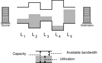
Figure 1: An Internet path with links characterized by different capacities and utilization levels.

Let $L_{i}$ be the $i$-th link of an Internet path, with $i\in{1..n}$. The capacity $C_{i}$ of the $i$-th link is the maximum data rate that link $L_{i}$ can achieve. The bottleneck capacity of an Internet path is defined as the capacity of the narrowest link of the path considered [15], and thus it is equal to $\min\{C_{1},...,C_{n}\}$ (in other words it is the capacity of the link that imposes a bottleneck on the path in terms of data rate). The capacity of a link (or a path) is a static property that does not change with time, and should not be confused with the available bandwidth. The latter represents the residual bandwidth not currently in use by other traffic (a property whose value depends on current conditions) [16, 17]. If $A_{i}(t)$ is the available bandwidth of $L_{i}$ at time $t$, then $C_{i}\geq A_{i}(t)$ holds. For example, the bottleneck capacity of the path shown in Figure 1 is $C_{3}$, the capacity of $L_{3}$, whereas the link with the smallest available bandwidth is $L_{5}$ (considering the current utilization level as depicted by the gray areas).

The ability to measure the bottleneck capacity is useful not only for network protocols (e.g. for congestion control) but also at the application and user levels. In fact, this information can be used to tune the operational parameters of streaming applications and peer-to-peer systems, or to evaluate the actual performance of a residential ISP connection.

Methods and techniques for measuring this network property have received significant attention from both researchers and practitioners  [18, 19, 20]. In addition, while most of the initial activities have been carried out for wired networks, more recently the study of techniques specifically designed for wireless environments has gained momentum [21, 22]. In this paper we move forwards in two different directions. On the one hand, we continue this trend by giving even more relevance to wireless scenarios. The aim is to make the evaluation of the bottleneck capacity more suitable for execution on mobile devices (smartphones and tablets, which have surpassed common PCs in terms of sales, now represent the preferred Internet-enabled devices for the majority of users). On the other hand, we believe that an evolution of bottleneck capacity estimation tools in a crowdsourcing perspective may pave the way for interesting and unexplored usages, as it may provide fine-grained information on today’s large scale networked systems.

The evaluation of the bottleneck capacity in a smartphone-based crowdsourcing scenario must take into account $i)$ bandwidth and energy efficiency, $ii)$ tuning for wireless connections, and $iii)$ support for possibly large numbers of users.

Bandwidth and energy efficiency. On smartphones and tablets, energy is a scarce resource and communication can be expensive. As a consequence, tools that do not consider these factors are likely to be abandoned by their users. Almost all the techniques designed and implemented so far have been conceived with the assumption that the devices are connected via wired links. Thus, they are not particularly efficient from this point of view.

In SmartProbe, the estimation of the bottleneck capacity has been designed to be suitable for mobile devices, with bandwidth efficiency as a primary goal. Reducing the amount of data transmitted and received, in turn, brings advantages in terms of energy efficiency. Our techniques considerably reduce the amount of traffic: up to 96% for 3G cellular networks and up to 89% for Wi-Fi networks.

Tuning for wireless connections. Most existing techniques do not behave properly in wireless scenarios, which tend to have high bit error rates. In addition, the tools currently available for smartphones implement rather trivial techniques: they perform an HTTP GET request and calculate the time needed to retrieve the requested page. However what is obtained is just an estimation of TCP throughput and not of bottleneck capacity. These are actually two different properties that should not be confused [17] (for instance, TCP throughput depends on a number of factors such as buffer size, round trip time, and retransmission errors).

SmartProbe introduces customizations to state-of-the-art techniques in order to operate more smoothly in wireless scenarios.

Support for possibly large numbers of users. The use of bottleneck estimation methods from a crowdsourcing perspective creates a new set of problems. Countermeasures are needed to prevent simultaneous measurements from interfering with each other.

SmartProbe tackles these problems by incorporating scheduling and queuing mechanisms (on the server-side) to support large numbers of users.

3 Estimation of bottleneck capacity: theory and state of the art

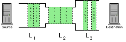
Figure 2: A pair of packets going through a set of links with different capacities.

Many capacity estimation techniques are based on the dispersion of a pair of packets. If link $i$ has capacity $C_{i}$, transmitting a packet with size $P$ on such link requires $\tau_{i}=P/C_{i}$. When two packets are sent back to back, they reach the receiver with a dispersion $D=P/C$, where dispersion is the time between the last bit of the first packet and the last bit of the second packet. If the transmission of the two packets entails going through $n$ links, the dispersion at the receiver will be $D=P/\min\{C_{1},...,C_{n}\}$. Thus, by measuring on the receiver the dispersion of a couple of packets with a known size, it is possible to calculate the bottleneck capacity [16, 18]. Figure 2 shows a pair of packets (PACK1 and PACK2) going through a set of links. The smaller the capacity of a link, the longer the time needed to transmit the packets. When the two packets reach the destination host the dispersion depends on the capacity of $L_{2}$, which is the narrowest link. This technique forms the basis of a large set of tools including, for instance, Pathrate [23] and CapProbe [19]). In general, this procedure is repeated several times (i.e. several packet pairs are sent) to obtain statistically significant results.

Systems based on the dispersion of packet pairs may be inaccurate in the presence of high speed links [20]. Capacity is estimated as $C=P/D$, but in high speed networks $C$ is large and $P$ is limited by the size of the Maximum Transmission Unit (MTU). As a consequence, $D$ becomes very small, which may lead to timer resolution problems. For example, let us consider a 1 Gbps network where MTU is 1500 B: in this case $D$ is equal to $12\mu s$, a value that cannot be easily measured with common system timers.

Another possible source of inaccuracy is interrupt coalescence, a technique in which Network Interface Cards (NICs) generate a single interrupt for multiple packets, when they are received in a short time interval [24]. With interrupt coalescence, $D$ gets reduced because of data buffering and, in the end, the resulting $C$ may be incorrect.

These problems are solved by enlarging the numerator of the above introduced equation, i.e. by sending a larger amount of data from source to destination. Since the MTU cannot be enlarged indefinitely, the only possibility is to send a larger number of packets. The capacity can thus be computed as:

$$C=\frac{(k-1)P}{D}$$ (1)

where $k$ is the size of the train and $D$ is now the dispersion between the first and last packet of the train.

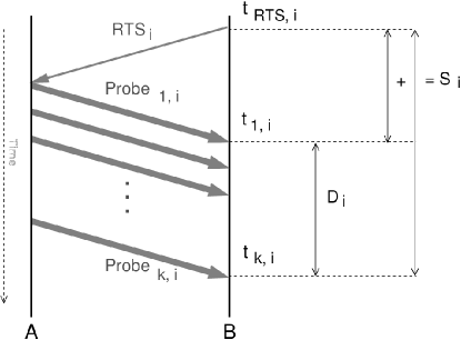
Figure 3: Delay sum components.

The presence of cross-traffic in the path – that is Internet traffic generated by other sources and dispatched by the same router(s) – can alter the dispersion values. This may lead to capacity estimation errors. Moreover, since packet trains are longer than packet pairs, techniques based on trains are more prone to this problem than the ones based on pairs.

Some tools include mechanisms for reducing the effects of external noise. PBProbe adopts the concept of delay sum to minimize the under- and over-estimations caused by cross-traffic. Figure 3 shows the estimation procedure in PBProbe. In particular, the bottleneck capacity is estimated along the path that goes from A to B. On receiving a Request To Send (RTS), A sends a train of probes to B. The delay sum for the $i$-th train, indicated as $S_{i}$, is computed as the sum of the delays experienced by the first and the last packet of that train. Thus, if $n$ trains are used, the minimum delay sum identifies the train that has experienced the minimum queuing delay. Once the train in a campaign with the minimum delay sum has been identified, the capacity is computed with Equation 1 using the dispersion $D$ experienced by such train.

PBProbe was originally designed to estimate the bottleneck capacity of high-speed wired networks, but it was also successfully used to infer the bottleneck capacity in wireless environments [20]. The consumption of resources is the main issue that prevents the direct adoption of PBProbe on mobile phones. To obtain a valid result, PBProbe uses $n=200$ trains, where each train is composed of $k$ packets of 1500 bytes. The larger the value of $k$, the larger the dispersion time $D$ experienced between the arrival of the first and last packet of each train and, as a consequence, the smaller the impact of potential interference phenomena caused by interrupt coalescence and by timer resolution. To identify the correct value of $k$, PBProbe compares the dispersion time $D$ registered by trains with a threshold value $D_{thresh}$: if any of the trains experience $D<D_{thresh}$, then the train length is increased tenfold and the computation starts again from scratch. In [20], $D_{thresh}=1$ ms is considered the minimum value able to limit the impact of system interferences. This means that PBProbe requires sending about two thousand packets, i.e. about 3 MB of data, to correctly compute the capacity of a 802.11g wireless network.

On devices with limited resources, such as smartphones, $D_{thresh}=1$ ms is not a realistic value. As discussed in the following (in Section 4.4), the impact of interference phenomena on these devices is acceptable when $D_{thresh}=10$ ms. In this case, PBProbe would require more than twenty thousand packets, i.e. about 30 MB of data, for a 802.11g network. In general, the amount of data produced by PBProbe to correctly infer the bottleneck capacity of mobile networks (assuming that $D_{thresh}$ is equal to 10 ms) is between about 300 KB and 300 MB. This often represents a problem: a large amount of transferred data is likely to lead to a significant consumption of energy and, depending on the commercial agreement between users and mobile operators, it may also lead to economic costs.

4 Estimating the bottleneck capacity on smartphones

This section presents an overview of the SmartProbe system and provides the details of the bottleneck estimation procedure.

4.1 System overview

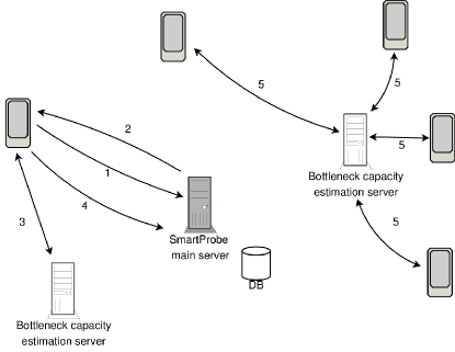
Figure 4: Overview of the system.

As previously mentioned, measuring the bottleneck capacity along a path requires active communication between the two endpoints. The source and destination hosts exchange a set of packets, usually called probes, and collect timestamps to infer this property of the network. The procedure is generally repeated several times to obtain accurate results.

Figure 4 shows a high-level overview of the SmartProbe system. A number of clients (smartphones) interact with the main server, which coordinates their activities and acts as collector of results. Other secondary servers are used as endpoints for bottleneck capacity estimation measurements. Each individual bottleneck capacity estimation server (BCES) is able to handle a number of clients.

When a user starts a measurement, the smartphone contacts the SmartProbe server (1) which replies with the address of the BCES to be used as the measurement endpoint (2). The selection of the best BCES can be based on the country of the device or its geographical coordinates. The client then performs the required operations by interacting with the given BCES (3). The result is the estimated bottleneck capacity along the path that goes from the client to the selected BCES. The measurement procedure is executed two times to obtain the bottleneck capacity for the two directions. Results are then forwarded by the client to the SmartProbe server (4), where they are saved onto persistent storage.

Measuring the bottleneck capacity does not require a large amount of time. However, given that the system is designed to operate in a crowdsourcing scenario, a single BCES has to cope with numerous users and it may be involved in multiple measurements at the same time (as depicted on the right-hand side of Figure 4). It is clear that without appropriate strategies, simultaneous measurements (5) could be compromised or distorted because of mutual interference. For this reason, BCESs include mechanisms for multiplexing and queuing measurement requests coming from different clients. These methods are described in Section 5.

SmartProbe is currently available as a service provided by the Portolan platform, a smartphone-based crowdsourcing system aimed at sensing large-scale networks. The SmartProbe functionalities, on the client-side, were incorporated as a module of the Portolan app, which besides bottleneck estimation provides other network tools (signal coverage maps and exploration of the graph of the Internet) [25, 26, 27]. The Portolan app (for Android), and thus also SmartProbe, is available for free on Google Play.

4.2 Protocol overview

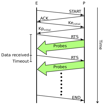
Figure 5: SmartProbe protocol.

The main steps of the bottleneck estimation procedure are shown in Figure 5. Initially, one of the two hosts operates as Estimator (E) – i.e. the host that asks for packets and computes the capacity – while the other acts as Prober (P), i.e. the host that waits for requests and sends packet trains. Each phase begins with an UDP handshake between Prober and Estimator to synchronize and initialize the two hosts, followed by the transmission of the train of UDP packets. The Estimator starts the handshake by sending a START message to the Prober, which replies with an ACK. After this, each host calculates the minimum $k$ that has to be used to compute the capacity without being affected by timer resolution and interrupt coalescence problems (see Section 4.5). The smallest $k$ is chosen for the measurement, since the slower link introduces a delay large enough to estimate the capacity correctly in both directions.

The Estimator then starts the measurement by sending an UDP control message named RTS (Request To Send), which triggers the dispatch of an UDP train. The RTS message contains the number of packets $k$ that the Prober has to use for the train it is going to send. The dispatch of every UDP control message also starts a timer that allows the two hosts to not stall in case of packet losses. Once the Estimator has correctly received all the packets of a train, it computes the dispersion and then the capacity (using Equation 1). Otherwise the train is invalidated when the timeout expires. If multiple failures are experienced, the two hosts assume that the network is congested and the experiment is restarted by halving the train length. The estimation is completed when n valid trains are received. When this happens an END message is sent by the Estimator to the Prober. Once finished, Prober and Estimator swap their roles and the procedure is repeated, to obtain an estimation of the bottleneck capacity in the opposite direction.

⬇

$i\leftarrow 0$

$failed\leftarrow 0$

$D_{min}\leftarrow+\infty$

$S_{min}\leftarrow+\infty$

$k\leftarrow k_{initial}$

while($i<n$)

Set timeout

Receive packet train $i$

if (timeout triggered)

$failed\leftarrow failed+1$

if ($failed==3$)

$i\leftarrow 0$

$failed\leftarrow 0$

$k\leftarrow max(\lfloor k/2\rfloor,2)$

$D_{min}\leftarrow+\infty$

$S_{min}\leftarrow+\infty$

continue

else

Measure $D_{i}$ and $S_{i}$

if ($S_{i}$ < $S_{min}$)

$S_{min}\leftarrow S_{i}$

$D_{min}\leftarrow D_{i}$

$i\leftarrow i+1$

Compute capacity with $D_{min}$

Figure 6: SmartProbe estimation algorithm.

The SmartProbe algorithm is expressed by the pseudo-code in Figure 6.

4.3 Dispersion and capacity

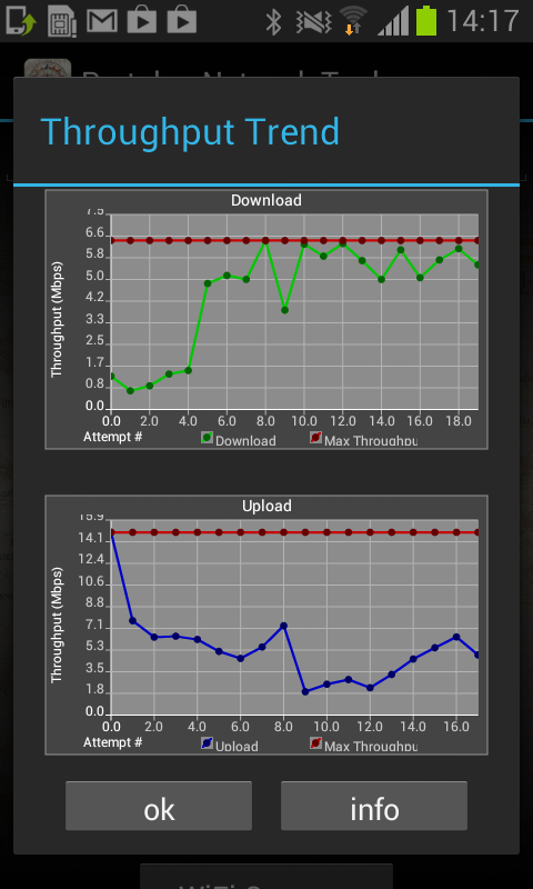
Figure 7: The capacity values obtained with the different trains are shown to the user.

SmartProbe computes dispersion according to a procedure that enhances the procedure based on delay sum. Let us call $t_{1,i}$ the delay registered by the first packet of the $i$-th train, and $t_{k,i}$ the delay of the last packet of the same train. Let us also define ${t_{1}}^{min}=\min t_{1,j},\quad j\in 1..i$, i.e. the minimum interval registered so far between a request to send and the arrival of the first packet of a train. The capacity value for the $i$-th train is then calculated using the dispersion value $D_{i}=t_{k,i}-{t_{1}}^{min}$, and applying Equation 1. A similar technique, for packet pairs, has also been presented in [28].

This approach has been followed because the value of capacity for the $i$-th train, calculated using $t_{k,i}-t_{1,i}$ as dispersion value, may generate an over-estimation due to compression phenomena [20]. In fact, a better estimate of the minimum time needed to receive the first packet of a train may be already available. In other words, we can state that if the first packet in a train experienced an arrival time larger than the minimum, then this is due to cross-traffic. Therefore, a more reliable estimation of the capacity, for the $i$-th attempt, is obtained when using $D_{i}=t_{k,i}-{t_{1}}^{min}$ as the dispersion value.

This procedure is repeated $n$ times (for all trains), then the capacity value corresponding to the minimum delay sum is selected as the one that best estimates the bottleneck.

Once the estimation is completed, the final results are shown to the user. Besides the bottleneck capacity values in upload/download, SmartProbe displays all the values computed during the estimation process. Figure 7 shows the measured capacity against the train number.

4.4 Selection of $D_{thresh}$ in a smartphone-based scenario

In previous literature, $D_{thresh}$ is set to 1 ms on the basis of experimental results obtained from wired servers. Unfortunately, this value cannot be directly applied to a smartphone-based scenario, as these devices are characterized by relatively scarce resources. Thus, we run a set of experiments aimed at finding the smallest $D_{thresh}$ value that provides an acceptable loss of accuracy (due to timer resolution and interrupt coalescence).

We followed an approach derived from the one described in [20]. In particular, we analyzed the accuracy of smartphone-based measurements in an unloaded Wi-Fi network. The experimental setup consisted of a smartphone connected to an 802.11g wireless network and a BCES on the same wired LAN of the wireless access point (Figure 8). We varied the value of $k$ to generate trains of increasing length (and thus characterized by increasing dispersion). For each train length, the measurement has been repeated 100 times. The results are depicted in Figure 9: the average result of the tool converges to a stable capacity value when using trains composed of more than 40 packets. This value of $k$, by applying Equation 1, leads to a dispersion value $D\sim 10$ ms, which we consider to be the minimum dispersion value $D_{thresh}$ on smartphones (the effects of operating system interferences are not negligible with smaller values).

4.5 SmartProbe bandwidth-saving features

SmartProbe includes bandwidth-saving features to make the estimation procedure compatible with resource-constrained devices.

4.5.1 Packet train length

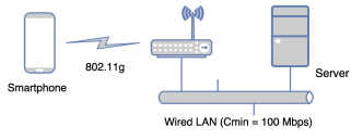
Figure 8: Experimental setup: the server is a Pentium 4, 2.80GHz machine equipped with 2 GB RAM running Linux Ubuntu 11.04, whereas the smartphone is a Samsung Galaxy Nexus GT-19250 running Android 4.0.3; both the server and the access point are on the same Ethernet LAN with 100Mbps NICs, while the smartphone is connected via 802.11g to the access point.

In PBProbe the value of $k$ is chosen dynamically by analyzing the dispersion time: if a train is received with a dispersion value lower than a predefined threshold $D_{thresh}=1$ ms, then $k$ is increased tenfold.

SmartProbe follows a different approach: the a priori knowledge about the type of network to which the smartphone is connected and the nominal capacity of that type of network are used to determine the initial value of $k$ ($k_{initial}$). The type of network the smartphone is connected to is directly provided by mobile operating systems. The nominal capacity typically represents an upper bound of the real wireless performance [29], thus it can be used to understand the minimum number of packets required to produce a dispersion value larger than $D_{thresh}$. The value of $k$ is dynamically lowered by SmartProbe whenever too many trains experience packet losses. This can be caused for example by the presence of traffic shapers on the link or by excessive contending traffic on the wireless access point. In these cases, the application still tries to retrieve the value of the bottleneck capacity by progressively lowering the value of $k$. The procedure stops when $k$ becomes equal to 2, i.e. when a simple packet pair is used.

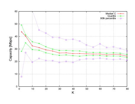
Figure 9: Stability of capacity estimation when varying the train length.

Table 1: Nominal capacity and initial train length per wireless technology.

Network		Cap. [Mbps]	$k_{initial}$
Wi-Fi 802.11	b	11	11
	a,g	54	46
	n	450	376
Mobile 2G	GPRS	0.171	2
	EDGE	0.473	2
Mobile 3G	UMTS	1.8	3
	HSPA	14.4	13
Mobile 4G	LTE	326.4	273

The initial value of $k$, from which the computation starts, is obtained by applying Equation 1, where $C$ is the nominal capacity of the network type currently in use, $P$ is 1500 B and $D$ is $D_{thresh}$. Table 1 summarizes the values of $k_{initial}$ for common wireless networks: the faster the network, the larger $k_{initial}$.

4.5.2 Number of trains per campaign

Another factor that makes previous techniques less usable on smartphones is that they use a fixed amount of trains for each measurement (e.g. 200 trains, as previously mentioned). To decrease the amount of traffic – and therefore the costs in terms of connection fees and battery consumption – n needs to be significantly reduced. We thus performed a campaign of 100 experiments with $n=200$. In each test we first retrieved the most reliable capacity $C^{200}$ using the full sample list. Then, we computed the capacity $C^{m}$ that would be obtained by considering only the first $m$ trains. Finally, we calculated the error between $C^{200}$ and $C^{m}$. Figure 10 shows the distribution of errors when varying $m$ (median value, inter-quartile and 90th percentile). The median value of the error becomes close to zero for $m\geq 60$, meaning that $n=m=60$ is sufficient to infer the correct capacity value most of the times. Obviously, reducing the number of trains leads to an unavoidable loss of accuracy. However in an environment where saving energy is fundamental, the choice of $n=60$ represents a good trade-off between accuracy and performance.

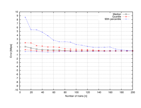
Figure 10: Error when varying the number of trains (with respect to 200 trains).

5 Supporting a large number of users

In a crowdsensing scenario, it is likely that multiple users will want to measure their bottleneck capacity simultaneously. This requires the presence of proper mechanisms on the server side, so that multiple estimations can be carried out without interfering with each other.

5.1 SmartProbe infrastructure: server side

The main problem in satisfying several requests at the same time is that the computation and traffic load generated by multiple clients may reduce the accuracy of measurements. In fact, requests from different sources converge to the same BCES using a single link (Figure 11). Similar problems may occur when multiple clients act as Estimators. For instance, suppose that one client sends an RTS to the server; if the server is busy because it is satisfying another request, it will not be able to respond immediately to the new client.

Figure 11: Bottleneck capacity estimation servers are connected to the Internet through a single link.

Figure 12: Activity diagram of scheduling

These problems can be avoided by preventing multiple clients from entering the active measurement phase at the same time. To this purpose, the server includes mechanisms for scheduling operations with clients. The execution time of a client action (i.e. sending a train of packets) depends both on its geographical position, which influences the RTT, and the connectivity type, as the length of the train changes with the type of network (Wi-Fi, UMTS, etc.). As a consequence, slower (or more distant) clients may keep the server busy more than faster (or closer) ones. Thus, each BCES adopts a Deficit Round Robin (DRR) scheduler for serving the requests coming from clients [30].

Each requesting client is represented as an independent flow of the DRR scheme, where each flow has its own queue (as shown in Figure 13). In other words, the list of flows/queues represents the set of clients currently involved in an estimation. When an estimation is completed, the associated queue is removed from the list. The size of the elements entering each DRR queue (using DRR terminology) corresponds to the time a given client is assumed to need to perform its next actions. Let $V_{net,i}$ be the time needed by client $i$, connected via network type $net$, to perform its next measurement. $V_{net,i}$ can be calculated as the RTT between the client considered and the server, plus the time it takes to send a train composed of $k$ packets, each $P$ bytes long, over a network with nominal capacity $C_{nom}$ (i.e., $V_{net,i}=RTT_{net}+(k_{net,i}*P)/C_{nom}$).

A Deficit Counter (DC) is associated with every queue. The scheduling algorithm is described by the diagram shown in Figure 12: the two depicted activities may occur in parallel and are event-triggered. When the server receives a connection request from a new client, a new queue is created and measurement operations are added to that queue (on the left-hand size of Figure 12). The size of operations is calculated as mentioned above. The new queue is then inserted in the list of currently managed clients. As soon as the list becomes non empty, the activity depicted in the right-hand side of Figure 12 is triggered. One of the queues is selected as the current one, and an amount equal to Quantum Size (QS) is added to the DC of that queue. If the value contained in DC is greater than the size of the head element of the current queue, the measurement operation can be executed, otherwise the next queue is processed. If the operation is executed, the amount corresponding to its size is removed from DC and the client is served. The just processed operation is removed from the queue. When a queue becomes empty it is removed from the list. If the list is not empty the next queue is processed, otherwise the server goes idle and waits for new connections from clients.

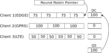
(a) Deficit round robin: QS is added to DC of the first queue.

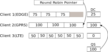
(b) Deficit round robin: the first element of the first queue is scheduled, QS is added to DC of the second queue.

Figure 13: Client operations are scheduled according to a Deficit Round Robin policy.

Figures 13a and 13b show a scenario where three clients are simultaneously interacting with the server. The three clients are connected to the Internet using different access technologies: EDGE, GPRS, and LTE. The duration of the probing operations is assumed to be equal to 100 with GSM, 75 with EDGE, and 50 with LTE. In Figure 13a a QS equal to 100 is added to the DC of the first queue, then the first element of this queue can be processed as the value of DC is greater than 75. The remaining amount (25) is left in DC for the next round (Figure 13b). The round robin pointer moves to the second queue and QS is added to its DC. Also in this case the value in DC is sufficient for processing the first element of the second queue (but in this case 0 will be left in DC). This procedure is repeated until all clients have completed their operations.

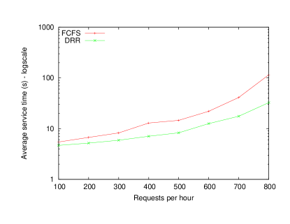
Figure 14: Service time with DRR and FCFS.

We studied the behavior of our DRR-based solution with respect to a system based on a First Come First Served (FCFS) policy. Evaluation was carried out through numerical analysis. The number of measurement requests per hour was varied between 100 and 800, to study the behavior of the two policies under different workloads. Communication between clients and server was characterized by RTTs uniformly distributed between 0 and 20 ms. In the considered scenario, all access technologies were equally represented. Figure 14 shows the obtained results in terms of service time (the amount of time between the time a request is issued by a client and the time the estimation is completed). As expected DRR and FCFS operate similarly when the the load is light: as soon as a request is received it can be immediately served, independently from the scheduling algorithm. On the contrary, when the load is high the differences between the two scheduling policies become significant. In particular, for the highest request rate, the service time with DRR is $\sim 70\%$ smaller than the one obtained with FCFS.

To have a DRR WorkQuotient equal to O(1), QS should be equal to the maximum time a client may need to perform an action (as specified in [30]). In our scenario, this could be done by using the parameters of the slowest (in terms of capacity value) connection the system has to cope with ($QS=RTT_{slowest}+(k_{slowest}*P)/C_{slowest}$), in practice by using the parameters of the GPRS connection. Nevertheless, we observed that selecting the value of QS according to this principle provides less benefits with respect to the ones shown in Figure 14, which have been obtained using a smaller value (approximately 1/3). This is explained by the fact that in our scenario flows are not backlogged, and thus using a smaller QS provides increased fairness.

6 Validation and experimental results

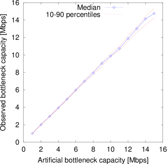
(a) Wi-Fi - download

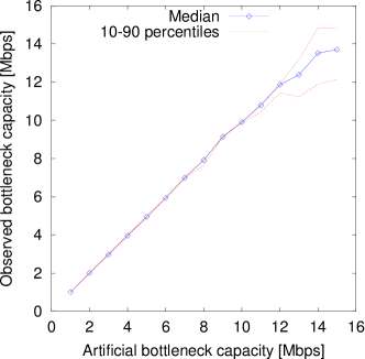
(b) Wi-Fi - upload

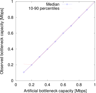
(c) Cellular - download

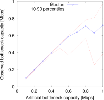
(d) Cellular - upload

Figure 15: Validation: observed bottleneck capacity against bandwidth limitation imposed on the server.

The mechanisms behind SmartProbe and their implementation were validated by measuring the bottleneck capacity in a scenario where the ground truth was known in advance. The scenario consisted of a smartphone running the SmartProbe client and a BCES connected to the Internet (Figure 8). The bandwidth of the connection between the BCES and the Internet was artificially limited to a set of known values using Dummynet [31]. In the first configuration, smartphone connectivity was obtained via Wi-Fi through a local access point. Results are shown in Figures 15a and 15b: for the considered range (1 Mbps - 15 Mbps) all the capacity values registered by SmartProbe perfectly correspond to the values set using Dummynet (for both directions). In the second configuration, the smartphone was connected to the Internet via its cellular interface. The considered range was 0.1 Mbps - 1 Mbps and the obtained results are shown in Figures 15c and 15d. Again, in download, the capacity value measured using SmartProbe exactly matches the bandwidth limitation imposed by Dummynet. In contrast, as far as upload is concerned, the measured value and the imposed value start to diverge when the artificial bandwidth limitation becomes greater than approximately 600 Kbps. This is due to the fact that SmartProbe measures the bottleneck capacity of the whole path between the smartphone and the BCES involved. In fact, when the limitation imposed by Dummynet is large, the bottleneck capacity is not located on the link that connects the server to the Internet, but on the cellular connection between the smartphone and the base station. Thus we can reasonably say that in all the considered cases SmartProbe was able to provide an exact measure of the bottleneck capacity (when the bottleneck is the artificial one on the link between BCES and the Internet) or a credible value (when the bottleneck is located on the uplink between the smartphone and the cellular base station).

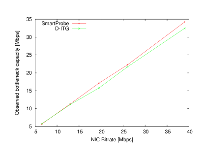
Figure 16: Validation when the bottleneck is located on the wireless link: capacities reported by SmartProbe and D-ITG.

To further validate SmartProbe, the system was also tested in a configuration where the link with narrowest capacity was the wireless one. This additional validation was carried out because in many real situations the wireless link acts as the bottleneck. The considered scenario is similar to the one depicted in Figure 8. The capacity of the wireless link was artificially restricted by forcing the bitrate of the wireless interface to specific values (the same approach has been used in [32]). The values we used correspond to five of the slowest supported bitrates of IEEE 802.11n. The capacity estimated by SmartProbe was compared to the one reported by D-ITG [33], which is not only a popular and reliable platform for generating traffic, but also a network measurement tool. Figure 16 shows the results averaged over ten repetitions (only download for the sake of brevity, same findings have been obtained for upload): the capacities reported by SmartProbe and D-ITG are very similar for all the considered modes of operation. The average absolute difference between the two tools is $\sim 3.9\%$. We believe this is a rather small value for this type of measurements, especially considering that the standard deviation of SmartProbe results is, on average, equal to $\sim 1.3\%$ of the reported capacity.

Table 2: SmartProbe: traffic generated in comparison with PBProbe.

Network		PBProbe [MB]	SmartProbe [MB]	SmartProbe worst case [MB]
Wi-Fi 802.11	b	3.3	1.0	1.6
	a,g	30.3	4.1	7.8
	n	300.5	33.8	67.1
Mobile 2G	GPRS	0.6	0.2	0.2
	EDGE	0.6	0.2	0.2
Mobile 3G	UMTS	3.3	0.3	0.4
	HSPA	30.3	1.2	2.2
Mobile 4G	LTE	300.5	24.6	48.8

We evaluated the bandwidth-saving characteristics of SmartProbe. To this purpose, we compared the amount of traffic generated by SmartProbe with the one produced by a technique based on the PBProbe algorithm. We considered $D_{thresh}=10$ ms for our smartphone-based scenario, as previously discussed.

Let us suppose that the bottleneck capacity is imposed by a 802.11g link. The technique based on PBProbe initially sends a train composed of two packets. The dispersion registered by such packet pair is below the threshold, thus the length of the train (excluding the first packet) is increased tenfold, and another train composed of eleven packets is sent. Also this train experiences a dispersion that is below the threshold, thus the length of the train is again increased tenfold. The train length is now sufficient for obtaining $D\geq D_{thresh}$ and other trains with the same length are sent until $n=200$ trains are received. This approximately generates 30.3 MB of data. SmartProbe starts the estimation using $n=60$ and $k=46$ (see Table 1) for a total of approximately 4.1 MB, about 13% of the traffic generated by PBProbe. In addition, even considering the worst case in which a persistent packet loss causes the length of packet trains to decrease to the smallest value, i.e. $k=2$, SmartProbe would require 7.8 MB of data, which is still 26% of data sent by PBProbe. Results for other types of wireless networks can be found in Table 2. The amount of traffic is reduced up to 96%. By sending a smaller amount of data, SmartProbe obtains obvious benefits in terms of battery consumption and economic costs.

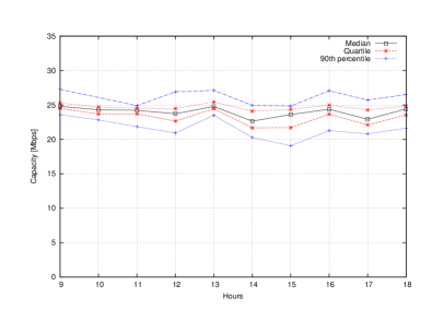
(a) Wi-Fi - download

(b) Wi-Fi - upload

Figure 17: Measurements in the presence of real background traffic.

Finally, SmartProbe was tested in presence of real background traffic. In this case, the bottleneck capacity of a Wi-Fi network was estimated several times to assess the stability of the results. Measurements were carried out during normal work hours, with a background traffic generated by 20-30 people. The experimental setup is the one shown in Figure 8. We performed 100 measurements every hour from 8AM to 4PM, with $n=60$, running the tool with variable network loads. Results are depicted in Figure 17 in terms of median, inter-quartile and 90th percentile. Results are quite stable around the median value, showing that SmartProbe is not strongly affected by the different levels of traffic encountered during the period considered.

7 Mapping the performance of mobile broadband operators with crowdsourcing

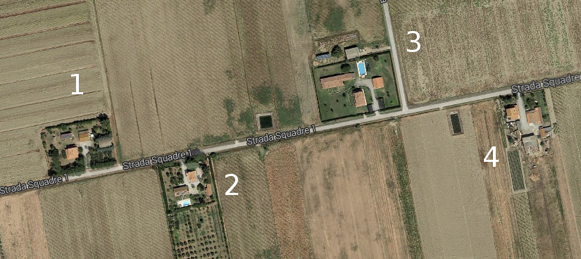
Figure 18: Mapping the performance of mobile broadband operators with crowdsourcing: considered area.

To demonstrate the use of SmartProbe in a crowdsourcing scenario, we implemented an application that maps the performance of mobile broadband operators with the help of the masses. Every time a user estimates the bottleneck capacity, the results are georeferenced and transferred to the main server, where they are saved onto persistent storage. When a large number of measurements are collected, these can be used to build a map that shows the real performance of mobile operators in relation to user positions. This information is obviously useful for future subscribers, as they may be interested in the real performance of operators in the area where they spend most of their time.

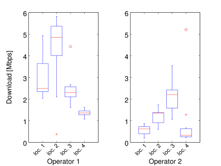
Figure 19: Mapping the performance of mobile broadband operators with crowdsourcing: results.

We used this proof-of-concept application to estimate the bottleneck capacity at different locations in a suburban area in Italy (Figure 18). For each location the bottleneck capacity was estimated using an Android smartphone connected to the Internet via two different mobile broadband operators (two of the major operators available in Italy, here indicated simply as “Operator 1” and “Operator 2”). In addition, for each operator the measurement was repeated ten times. Figure 19 shows the performance of the two operators (only downlink for the sake of brevity) at the four selected locations (which correspond to four houses). In all cases, Operator 1 provides the best performance. This demonstrates that if a measurement is collected at a given location, the result is reasonably stable and can be useful for all possible future subscribers who live in the surrounding areas.

8 Long term evaluation

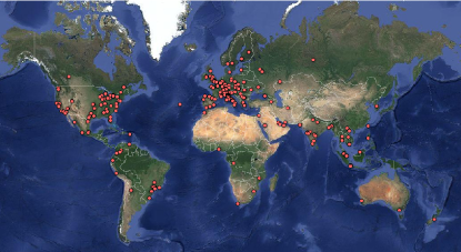
Figure 20: Location of SmartProbe users.

At the time of writing, SmartProbe has been operational for approximately one year. The geographical distribution of SmartProbe users is depicted in Figure 20 (more in detail, it represents the locations where measurements have been carried out). The majority of users is located in Europe and North America, with several users also in South America and Asia. Africa and Oceania are, on the contrary, not much represented. As already mentioned, results are sent to a central server where they are saved onto persistent storage. To preserve users’ privacy the ID of the device is anonymized and no personal information is transferred to the server.

Table 3: Normalized number of measurements per access technology (%).

GPRS	0.1
EDGE	1.1
UMTS	4.6
HSUPA	0.5
HSDPA	8.6
EVDO_A	4.9
EVDO_B	4.6
EHRPD	2.3
WI-FI	73.8

The normalized number of measurements, for the different access technologies, is reported in Table 3. The number of measurements carried out using declining cellular technologies (GPRS and EDGE) is quite limited. Approximately 1/4 of the measurements have been carried out using 3G technologies and the remaining ones concern Wi-Fi links.

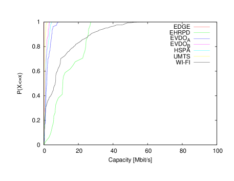
(a) Upload

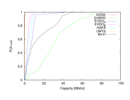
(b) Download

Figure 21: Upload and download capacity (CDF) collected during approximately one year of operation.

Figure 21 shows the cumulative distribution function of upload and download capacity as registered by the users of SmartProbe during the period of operation. The total number of measurements is  3350:  1730 for upload and  1620 for download. Measurements include both Wi-Fi connections and cellular connections (these latter are grouped by access technology). As expected, 3G technologies provide the best results for cellular connections and with EHRPD the download capacity is even larger than Wi-Fi.

These results must be interpreted as a first outcome of the crowdsourcing-based technique we propose. In any case, even considering the limited period, they clearly demonstrate that aggregating information collected by volunteers, to provide global metrics in terms of bottleneck capacity, is feasible. Obviously, a deeper and more detailed analysis will be possible when a larger amount of measurements are available. It is worthwhile to remember that all the measurements have been triggered by real users who voluntarily joined the system. As known, increasing the number of participants in a crowdsensing scenario is not easy, as specific incentive mechanisms have to be designed and put into practice (but this is outside the scope of this work) [34].

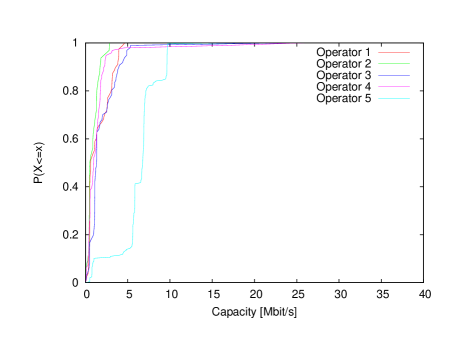
(a) Upload

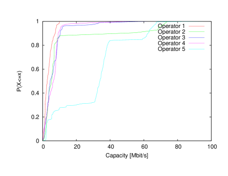
(b) Download

Figure 22: Upload and download capacity (CDF) of major Italian cellular operators.

Figure 22 shows the bottleneck capacity registered when using the five largest Italian mobile broadband operators. This kind of analysis has been restricted to Italy because for other countries the amount of measurements do not allow us to draw statistically sound conclusions. As evident, one of the operators provides significantly better performance in terms of both upload and download capacity. Although these results, at this stage, cannot be used to perform a thorough comparison of cellular operators, they already provide a first insight of the diffusion of cellular technologies among the considered companies. In general, a country-wide analysis like this can be used by customers to be informed about the global performance of operators. On the other side, an annotated map like the one presented in Section 7 can be extremely useful to obtain geographic-dependent information.

9 Related work

This section summarizes the most significant work related to the estimation of bottleneck capacity and to the use of crowdsourcing for network measuring.

9.1 Estimation of bottleneck capacity

The first tool focusing on the discovery of the bottleneck capacity was developed by Van Jacobson in 1997. Since then, a plethora of tools have been developed for wired networks, typically based on packet pairs (e.g. Bprobe [35], Pathrate [18], CapProbe [19] and TOPP [36]) and packet trains (e.g. PBProbe [20] and Cprobe [35]). Since these tools are not conceived for wireless environments, the results can in some cases be inaccurate. Recently, some dedicated tools based on packet pairs have been developed to infer the bottleneck capacity of wireless links (e.g. WBest [22] and AdHoc-Probe [21]). However as these tools are based on packet pairs, they can suffer from compression and expansion phenomena. Tools based on packet trains are able to minimize the effects of interrupt coalescence and timer resolution, but they still suffer from contending traffic interference. Of all these methods, PBProbe is the best performer on wireless networks [20]. However, as already stated, the amount of traffic generated by PBProbe is not optimized, and its use on smartphones is resource-demanding. To the best of our knowledge, SmartProbe is the first attempt towards a full adaptation of bottleneck capacity estimation techniques to the smartphone platform. The only tools for smartphones implemented so far are focused on estimating the bulk transfer capacity [37], i.e. the amount of data that can be sent between two ends via TCP (which, as already discussed in Section 3, is different from the bottleneck capacity [15]).

One of the first works where the problem of measuring the bandwidth is contextualized to a wireless scenario is the one by Johnsson et al. [38]. In particular, the authors discuss the effects caused by the probe packet size and cross-traffic on the estimation process when 802.11 wireless links are used.

A performance assessment of four tools for capacity estimation when operating on 802.11 links is presented in [39]. Experiments have been carried out in a semi-anechoic chamber, in order to evaluate the tools in a controlled and interference-free environment. Repeatability of procedures and the use of a digital storage oscilloscope allowed the authors to collect extremely accurate timestamps and to deeply study the interaction between capacity estimation tools and network interface cards.

9.2 Crowdsourcing for evaluating network properties

The crowdsourcing approach has been used to evaluate and measure network properties both in wired and wireless scenarios.

DIMES is a distributed measurement infrastructure that collects information on the topology of the Internet and its evolution [12]. The key idea behind DIMES is a shift from dedicated measurement architectures to a large community of volunteers: each participant runs a monitoring agent that carries out traceroute- and ping-based campaigns, then results are aggregated to produce a map at the autonomous system level of abstraction. Besides parallelization of workload, the heterogeneity of participants in terms of location provides the opportunity to measure the Internet from different points of view. This is a significant improvement compared to solutions characterized by a relatively small number of vantage points. In summary, crowdsourcing is beneficial not only in terms of raw power, but also because of the specific nature of every individual participant.

Dasu is an experimentation platform that supports measurement activities at the Internet’s edge on end user machines [13]. Dasu has been implemented as an extension of a peer-to-peer client (BitTorrent) to leverage its popularity and wide coverage. An experiment administrator can assign tasks to the participating clients. The measurement activities to be executed on user devices are specified through simple “when-then” rules and comprise both active tools (ping, traceroute, etc.) and passive data collectors. The availability of a large number of cooperating users supports the execution of large scale experiments aimed at studying routing asymmetry and Internet topology.

Similarly, crowdsourcing has been used to detect service-level network events [40], and to characterize ISPs and evaluate their performance [41]. Also in these cases, the BitTorrent client has been adopted as the implementation platform, since P2P sessions are network-intensive (this enables the passive collection of information) and characterized by long sessions (thus providing extensive monitoring periods). The unique perspective of participants and the involvement of a large number of end-users enable the collection of an unprecedented amount of information on the status of the network, especially at the edges of the Internet.

BSense is a system aimed at creating maps concerning the quality of broadband connections [42]. The system relies on a software agent that is executed on broadband users’ machines. The agent periodically measures the latency, packet loss rate, and bandwidth of the broadband connections, then it uploads the obtained results onto the BSense server. The framework has been tested with the help of 60 volunteers located in a Scotland region. Differently from SmartProbe, BSense is not specifically designed for estimating capacity in a wireless scenario: the default configuration for the download and upload sessions uses 8 concurrent UDP/TCP flows at 400 packets/s, with 1024 byte packets.

A large study about broadband performance is presented in [43]: latency, packet loss, and throughput measurements have been collected from nearly 4000 users and across 16 ISPs in USA. The largest part of monitored homes relies on gateways specifically deployed for studying network performance from the point of view of residential users. In particular, running experiments from such vantage points enables fine grained control on confounding factors, such as cross traffic or home wireless networks.

Hobbit is a measurement platform for broadband monitoring [44]. The platform includes measurements clients executed on users’ machines, measurement servers that cooperate with clients, and a management server for coordinating activities, planning experiments, and collecting results. A deployment of 400 clients has been used to study the performance of a set of ISPs in terms of fixed broadband access.

We believe that SmartProbe represents a significant addition to the landscape depicted above: it shares with these systems the key idea of using people as a means for evaluating the properties of large-scale networks with limited efforts, and expands existing work with bottleneck estimation in a wireless scenario.

Cognitive radios (CRs) are intelligent wireless communication systems that adapt their behavior to changing spectral conditions [45]. By automatically adapting their parameters of operation to the network status, CRs are able to more efficiently use the radio spectrum and to provide reliable communication [46]. In [47], the authors discuss the use of radio environmental maps (REMs) for cognitive wireless regional area networks. REMs operate as an integrated database that characterizes the radio environment using geographical information, spectral regulations, location and activities of radios, and policies. REMs are updated using observations produced by CR nodes, which in turn receive relevant information through the CR network itself. To a certain extent, part of the content of REMs is generated according to the crowdsourcing paradigm. Similar ideas are also discussed in [48, 49].

At first glance, these maps and the one produced by SmartProbe could be considered as similar. However, a more extensive analysis makes it clear that the purpose of REMs and SmartProbe maps is totally different and that the two systems operate on completely separate levels. In fact, REMs provide information used to tune the operational parameters at the lower levels of the networking stack (mostly the physical layer and the data link layer); the aim is to improve performance or to make efficient use of the spectrum. In contrast, the system we propose produces information dedicated to the user level and is completely independent of the underlying communication technologies and protocols. Unlike CRs, SmartProbe does not improve communication efficiency; instead it provides answers to questions like “which cellular operator performs best in an area of interest?”. Answers are provided using information generated by other users via crowdsourcing.

10 Conclusions

The mobile crowdsensing paradigm can be extremely useful for analyzing the characteristics of large-scale networks. With the help of the masses it is now possible to collect an unprecedented amount of information on the performance of networked systems. At the same time, the mobility of users and devices makes it possible to analyze large networks from a geographical point of view. However, these opportunities come at the cost of increased technical complexity. Smartphones are resource-constrained devices, especially from the point of view of energy and communication costs, and thus specific energy- and bandwidth-saving techniques need to be designed and put into practice. Protocols need to cope with a possibly large number of users and the back-end infrastructure has to store and process huge amounts of data.

We have described the design and implementation of a mobile crowdsourcing system aimed at measuring the bottleneck capacity of Internet paths. SmartProbe generates less traffic than similar tools, in order not to compromise the user experience, and includes server-side mechanisms to support simultaneous measurement requests. The presented application demonstrates that a collective and georeferenced evaluation of the performance of mobile broadband operators can be used to support intelligent user decisions.

References

- [1] J. Howe, Crowdsourcing: Why the Power of the Crowd Is Driving the Future of Business, Random House, 2008.
- [2] Threadless, http://www.threadless.com (2015).
- [3] SETI@Home, http://setiathome.berkeley.edu (2015).
- [4] Amazon, Mechanical Turk, http://www.mturk.com (2015).
- [5] Microworkers, http://www.microworkers.com (2015).
- [6] Crowdflower, http://www.crowdflower.com (2015).
-
[7]
A. Doan, R. Ramakrishnan, A. Y. Halevy,