Support Vector Machines under Adversarial Label Contamination

Abstract

Machine learning algorithms are increasingly being applied in security-related tasks such as spam and malware detection, although their security properties against deliberate attacks have not yet been widely understood. Intelligent and adaptive attackers may indeed exploit specific vulnerabilities exposed by machine learning techniques to violate system security. Being robust to adversarial data manipulation is thus an important, additional requirement for machine learning algorithms to successfully operate in adversarial settings. In this work, we evaluate the security of Support Vector Machines (SVMs) to well-crafted, adversarial label noise attacks. In particular, we consider an attacker that aims to maximize the SVM’s classification error by flipping a number of labels in the training data. We formalize a corresponding optimal attack strategy, and solve it by means of heuristic approaches to keep the computational complexity tractable. We report an extensive experimental analysis on the effectiveness of the considered attacks against linear and non-linear SVMs, both on synthetic and real-world datasets. We finally argue that our approach can also provide useful insights for developing more secure SVM learning algorithms, and also novel techniques in a number of related research areas, such as semi-supervised and active learning.

1 Introduction

Machine learning and pattern recognition techniques are increasingly being adopted in security applications like spam, intrusion and malware detection, despite their security to adversarial attacks has not yet been deeply understood. In adversarial settings, indeed, intelligent and adaptive attackers may carefully target the machine learning components of a system to compromise its security. Several distinct attack scenarios have been considered in a recent field of study, known as adversarial machine learning [1, 2, 3, 4]. For instance, it has been shown that it is possible to gradually poison a spam filter, an intrusion detection system, and even a biometric verification system (in general, a classification algorithm) by exploiting update mechanisms that enable the adversary to manipulate some of the training data [5, 6, 7, 8, 9, 10, 11, 12, 13]; and that the detection of malicious samples by linear and even some classes of non-linear classifiers can be evaded with few targeted manipulations that reflect a proper change in their feature values [14, 13, 15, 16, 17]. Recently, poisoning and evasion attacks against clustering algorithms have also been formalized to show that malware clustering approaches can be significantly vulnerable to well-crafted attacks [18, 19].

Research in adversarial learning not only investigates the security properties of learning algorithms against well-crafted attacks, but it also focuses on the development of more secure learning algorithms. For evasion attacks, this has been mainly achieved by explicitly embedding knowledge into the learning algorithm of the possible data manipulation that can be performed by the attacker, e.g., using game-theoretical models for classification [15, 20, 21, 22], probabilistic models of the data distribution drift under attack [23, 24], and even multiple classifier systems [25, 26, 27]. Poisoning attacks and manipulation of the training data have been differently countered with data sanitization (i.e., a form of outlier detection) [28, 5, 6], multiple classifier systems [29], and robust statistics [7]. Robust statistics have also been exploited to formally show that the influence function of SVM-like algorithms can be bounded under certain conditions [30]; e.g., if the kernel is bounded. This ensures some degree of robustness against small perturbations of training data, and it may be thus desirable also to improve the security of learning algorithms against poisoning.

In this work, we investigate the vulnerability of SVMs to a specific kind of training data manipulation, i.e., worst-case label noise. This can be regarded as a carefully-crafted attack in which the labels of a subset of the training data are flipped to maximize the SVM’s classification error. While stochastic label noise has been widely studied in the machine learning literature, to account for different kinds of potential labeling errors in the training data [31, 32], only a few works have considered adversarial, worst-case label noise, either from a more theoretical [33] or practical perspective [34, 35]. In [31, 33] the impact of stochastic and adversarial label noise on the classification error have been theoretically analyzed under the probably-approximately-correct learning model, deriving lower bounds on the classification error as a function of the fraction of flipped labels $\eta$; in particular, the test error can be shown to be lower bounded by $\eta/(1-\eta)$ and $2\eta$ for stochastic and adversarial label noise, respectively. In recent work [34, 35], instead, we have focused on deriving more practical attack strategies to maximize the test error of an SVM given a maximum number of allowed label flips in the training data. Since finding the worst label flips is generally computationally demanding, we have devised suitable heuristics to find approximate solutions efficiently. To our knowledge, these are the only works devoted to understanding how SVMs can be affected by adversarial label noise.

From a more practical viewpoint, the problem is of interest as attackers may concretely have access and change some of the training labels in a number of cases. For instance, if feedback from end-users is exploited to label data and update the system, as in collaborative spam filtering, an attacker may have access to an authorized account (e.g., an email account protected by the same anti-spam filter), and manipulate the labels assigned to her samples. In other cases, a system may even ask directly to users to validate its decisions on some submitted samples, and use them to update the classifier (see, e.g., PDFRate, an online tool for detecting PDF malware [36]). The practical relevance of poisoning attacks has also been recently discussed in the context of the detection of malicious crowdsourcing websites that connect paying users with workers willing to carry out malicious campaigns (e.g., spam campaigns in social networks) — a recent phenomenon referred to as crowdturfing. In fact, administrators of crowdturfing sites can intentionally pollute the training data used to learn classifiers, as it comes from their websites, thus being able to launch poisoning attacks [37].

In this paper, we extend our work on adversarial label noise against SVMs [34, 35] by improving our previously-defined attacks (Sects. 3.1 and 3.3), and by proposing two novel heuristic approaches. One has been inspired from previous work on SVM poisoning [12] and incremental learning [38, 39], and makes use of a continuous relaxation of the label values to greedily maximize the SVM’s test error through gradient ascent (Sect. 3.2). The other exploits a breadth first search to greedily construct sets of candidate label flips that are correlated in their effect on the test error (Sect. 3.4). As in [34, 35], we aim at analyzing the maximum performance degradation incurred by an SVM under adversarial label noise, to assess whether these attacks can be considered a relevant threat. We thus assume that the attacker has perfect knowledge of the attacked system and of the training data, and left the investigation on how to develop such attacks having limited knowledge of the training data to future work. We further assume that the adversary incurs the same cost for flipping each label, independently from the corresponding data point. We demonstrate the effectiveness of the proposed approaches by reporting experiments on synthetic and real-world datasets (Sect. 4). We conclude in Sect. 5 with a discussion on the contributions of our work, its limitations, and future research, also related to the application of the proposed techniques to other fields, including semi-supervised and active learning.

2 Support Vector Machines and Notation

We revisit here structural risk minimization and SVM learning, and introduce the framework that will be used to motivate our attack strategies for adversarial label noise.

In risk minimization, the goal is to find a hypothesis $f:\mathcal{X}\to\mathcal{Y}$ that represents an unknown relationship between an input $\mathcal{X}$ and an output space $\mathcal{Y}$, captured by a probability measure $P$. Given a non-negative loss function $\ell:\mathcal{Y}\times\mathcal{Y}\to\mathbb{R}$ assessing the error between the prediction $\hat{y}$ provided by $f$ and the true output $y$, we can define the optimal hypothesis $f^{\star}$ as the one that minimizes the expected risk $R\left(\@ifmtarg{f}{\cdot}{f},\@ifmtarg{P}{\cdot}{P}\right)=\mathbb{E}_{(\mathbf{x},y)\sim P}\@ifmtarg{}{\left[\@ifmtarg{\ell\left(\@ifmtarg{f(\mathbf{x})}{\cdot}{f(\mathbf{x})},\@ifmtarg{y}{\cdot}{y}\right)}{\cdot}{\ell\left(\@ifmtarg{f(\mathbf{x})}{\cdot}{f(\mathbf{x})},\@ifmtarg{y}{\cdot}{y}\right)}\right]}{\left[\vphantom{}\@ifmtarg{\ell\left(\@ifmtarg{f(\mathbf{x})}{\cdot}{f(\mathbf{x})},\@ifmtarg{y}{\cdot}{y}\right)}{\cdot}{\ell\left(\@ifmtarg{f(\mathbf{x})}{\cdot}{f(\mathbf{x})},\@ifmtarg{y}{\cdot}{y}\right)}\;\right|\left.\,\vphantom{\@ifmtarg{\ell\left(\@ifmtarg{f(\mathbf{x})}{\cdot}{f(\mathbf{x})},\@ifmtarg{y}{\cdot}{y}\right)}{\cdot}{\ell\left(\@ifmtarg{f(\mathbf{x})}{\cdot}{f(\mathbf{x})},\@ifmtarg{y}{\cdot}{y}\right)}}\right]}$ over the hypothesis space $\mathcal{F}$, i.e., $f^{\star}=\operatornamewithlimits{\arg\,\min}_{f\in\mathcal{F}}R\left(\@ifmtarg{f}{\cdot}{f},\@ifmtarg{P}{\cdot}{P}\right)$. Although $P$ is not usually known, and thus $f^{\star}$ can not be computed directly, a set $\mathcal{D}_{\textrm{tr}}=\left\{(\mathbf{x}_{i},y_{i})\right\}_{i=1}^{n}$ of i.i.d. samples drawn from $P$ are often available. In these cases a learning algorithm $\mathfrak{L}$ can be used to find a suitable hypothesis. According to structural risk minimization [40], the learner $\mathfrak{L}$ minimizes a sum of a regularizer and the empirical risk over the data:

$$\mathfrak{L}(\mathcal{D}_{\textrm{tr}})=\operatornamewithlimits{\arg\,\min}_{f\in\mathcal{F}}\quad \left[\Omega\left(\@ifmtarg{f}{\cdot}{f}\right)+C\cdot\hat{R}\left(\@ifmtarg{f}{\cdot}{f},\@ifmtarg{\mathcal{D}_{\textrm{tr}}}{\cdot}{\mathcal{D}_{\textrm{tr}}}\right)\right]\,,$$ (1)

where the regularizer $\Omega\left(\@ifmtarg{f}{\cdot}{f}\right)$ is used to penalize excessive hypothesis complexity and avoid overfitting, the empirical risk $\hat{R}\left(\@ifmtarg{f}{\cdot}{f},\@ifmtarg{\mathcal{D}_{\textrm{tr}}}{\cdot}{\mathcal{D}_{\textrm{tr}}}\right)$ is given by $\frac{1}{n}\sum_{i=1}^{n}\ell\left(\@ifmtarg{f(\mathbf{x}_{i})}{\cdot}{f(\mathbf{x}_{i})},\@ifmtarg{y_{i}}{\cdot}{y_{i}}\right)$, and $C>0$ is a parameter that controls the trade-off between minimizing the empirical loss and the complexity of the hypothesis.

The SVM is an example of a binary linear classifier developed according to the aforementioned principle. It makes predictions in $\mathcal{Y}=\{-1,+1\}$ based on the sign of its real-valued discriminant function $f(\mathbf{x})=\mathbf{w}^{\top}\mathbf{x}+b$; i.e., $\mathbf{x}$ is classified as positive if $f(\mathbf{x})\geq 0$, and negative otherwise. The SVM uses the hinge loss $\ell\left(\@ifmtarg{f(\mathbf{x})}{\cdot}{f(\mathbf{x})},\@ifmtarg{y}{\cdot}{y}\right)=\max\left(0,1-yf(\mathbf{x})\right)$ as a convex surrogate loss function, and a quadratic regularizer on $\mathbf{w}$, i.e., $\Omega\left(\@ifmtarg{f}{\cdot}{f}\right)=\frac{1}{2}\mathbf{w}^{\top}\mathbf{w}$. Thus, SVM learning can be formulated according to Eq. (1) as the following convex quadratic programming problem:

$$\min_{\mathbf{w},b}\quad \tfrac{1}{2}\mathbf{w}^{\top}\mathbf{w}+C\textstyle\sum_{i=1}^{n}\max\left(0,1-y_{i}f(\mathbf{x}_{i})\right)\enspace.$$ (2)

An interesting property of SVMs arises from their dual formulation, which only requires computing inner products between samples during training and classification, thus avoiding the need of an explicit feature representation. Accordingly, non-linear decision functions in the input space can be learned using kernels, i.e., inner products in implicitly-mapped feature spaces. In this case, the SVM’s decision function is given as $f(\mathbf{x})=\sum_{i=1}^{n}\alpha_{i}y_{i}k(\mathbf{x},\mathbf{x}_{i})+b$, where $k(\mathbf{x},\mathbf{z})=\phi(\mathbf{x})^{\top}\phi(\mathbf{z})$ is the kernel function, and $\phi$ the implicit mapping. The SVM’s dual parameters $(\boldsymbol{\alpha},b)$ are found by solving the dual problem:

$$\min_{0\leq\boldsymbol{\alpha}\leq C} \frac{1}{2}\boldsymbol{\alpha}^{\top}\mathbf{Q}\boldsymbol{\alpha}-\mathbf{1}^{\top}\boldsymbol{\alpha}\enspace,\enspace{\rm s.t.}\enspace\mathbf{y}^{\top}\boldsymbol{\alpha}=0\enspace,$$ (3)

where $\mathbf{Q}=\mathbf{y}\mathbf{y}^{\top}\circ\mathbf{K}$ is the label-annotated version of the (training) kernel matrix $\mathbf{K}$. The bias $b$ is obtained from the corresponding Karush-Kuhn-Tucker (KKT) conditions, to satisfy the equality constraint $\mathbf{y}^{\top}\boldsymbol{\alpha}=0$ (see, e.g., [41]).

In this paper, however, we are not only interested in how the hypothesis is chosen but also how it performs on a second validation or test dataset $\mathcal{D}_{\textrm{vd}}$, which may be generally drawn from a different distribution $Q$. We thus define the error measure

$$V_{\mathfrak{L}}\left(\@ifmtarg{\mathcal{D}_{\textrm{tr}}}{\cdot}{\mathcal{D}_{\textrm{tr}}},\@ifmtarg{\mathcal{D}_{\textrm{vd}}}{\cdot}{\mathcal{D}_{\textrm{vd}}}\right) =\|f_{\mathcal{D}_{\textrm{tr}}}\|^{2}+C\cdot\hat{R}\left(\@ifmtarg{f_{\mathcal{D}_{\textrm{tr}}}}{\cdot}{f_{\mathcal{D}_{\textrm{tr}}}},\@ifmtarg{\mathcal{D}_{\textrm{vd}}}{\cdot}{\mathcal{D}_{\textrm{vd}}}\right)\enspace,$$ (4)

which implicitly uses $f_{\mathcal{D}_{\textrm{tr}}}=\mathfrak{L}(\mathcal{D}_{\textrm{tr}})$. This function evaluates the structural risk of a hypothesis $f_{\mathcal{D}_{\textrm{tr}}}$ that is trained on $\mathcal{D}_{\textrm{tr}}$ but evaluated on $\mathcal{D}_{\textrm{vd}}$, and will form the foundation for our label flipping approaches to dataset poisoning. Moreover, since we are only concerned with label flips and their effect on the learner we use the notation $V_{\mathfrak{L}}\left(\@ifmtarg{\mathbf{z}}{\cdot}{\mathbf{z}},\@ifmtarg{\mathbf{y}}{\cdot}{\mathbf{y}}\right)$ to denote the above error measure when the datasets differ only in the labels $\mathbf{z}$ used for training and $\mathbf{y}$ used for evaluation; i.e., $V_{\mathfrak{L}}\left(\@ifmtarg{\mathbf{z}}{\cdot}{\mathbf{z}},\@ifmtarg{\mathbf{y}}{\cdot}{\mathbf{y}}\right)=V_{\mathfrak{L}}\left(\@ifmtarg{\;\{(\mathbf{x}_{i},z_{i})\}\;}{\cdot}{\;\{(\mathbf{x}_{i},z_{i})\}\;},\@ifmtarg{\;\{(\mathbf{x}_{i},y_{i})\}\;}{\cdot}{\;\{(\mathbf{x}_{i},y_{i})\}\;}\right)$.

3 Adversarial Label Flips on SVMs

In this paper we aim at gaining some insights on whether and to what extent an SVM may be affected by the presence of well-crafted mislabeled instances in the training data. We assume the presence of an attacker whose goal is to cause a denial of service, i.e., to maximize the SVM’s classification error, by changing the labels of at most $L$ samples in the training set. Similarly to [35, 12], the problem can be formalized as follows.

We assume there is some learning algorithm $\mathfrak{L}$ known to the adversary that maps a training dataset into hypothesis space: $\mathfrak{L}:(\mathcal{X}\times\mathcal{Y})^{n}\to\mathcal{F}$. Although this could be any learning algorithm, we consider SVM here, as discussed above. The adversary wants to maximize the classification error (i.e., the risk), that the learner is trying to minimize, by contaminating the training data so that the hypothesis is selected based on tainted data drawn from an adversarially selected distribution $\hat{P}$ over $\mathcal{X}\times\mathcal{Y}$. However, the adversary’s capability of manipulating the training data is bounded by requiring $\hat{P}$ to be within a neighborhood of (i.e., “close to”) the original distribution $P$.

For a worst-case label flip attack, the attacker is restricted to only change the labels of training samples in $\mathcal{D}_{\textrm{tr}}$ and is allowed to change at most $L$ such labels in order to maximally increase the classification risk of $\mathfrak{L}$ — $L$ bounds the attacker’s capability, and it is fixed a priori. Thus, the problem can be formulated as

$$\mathbf{y}^{\prime}=\operatornamewithlimits{\arg\,\max}_{\mathbf{z}\in\mathcal{Y}^{n}}\quad R\left(\@ifmtarg{f_{\mathbf{z}}(\mathbf{x})}{\cdot}{f_{\mathbf{z}}(\mathbf{x})},\@ifmtarg{P}{\cdot}{P}\right)\enspace,$$ (5)

s.t. $$f_{\mathbf{z}}=\mathfrak{L}\left(\{(\mathbf{x}_{i},z_{i})\}_{i=1}^{n}\right)\enspace,$$

$$\textstyle\sum_{i=1}^{n}\mathbbm{I}[z_{i}\neq y_{i}]\leq L\enspace,$$

where $\mathbbm{I}[$] is the indicator function, which returns one if the argument is true, and zero otherwise. However, as with the learner, the true risk $R$ cannot be assessed because $P$ is also unknown to the adversary. As with the learning paradigm described above, the risk used to select $\mathbf{y}^{\prime}$ can be approximated using by the regularized empirical risk with a convex loss. Thus the objective in Eq. (5) becomes simply $V_{\mathfrak{L}}\left(\@ifmtarg{\mathbf{z}}{\cdot}{\mathbf{z}},\@ifmtarg{\mathbf{y}}{\cdot}{\mathbf{y}}\right)$ where, notably, the empirical risk is measured with respect to the true dataset $\mathcal{D}_{\textrm{tr}}$ with the original labels. For the SVM and hinge loss, this yields the following program:

$$\max_{\mathbf{z}\in\{-1,+1\}^{n}}\quad \tfrac{1}{2}\boldsymbol{\alpha}^{\top}\mathbf{Q}\boldsymbol{\alpha}+C\textstyle\sum_{i=1}^{n}\max(0,1-y_{i}f_{\mathbf{z}}(\mathbf{x}_{i}))\enspace,$$ (6)

s.t. $$(\boldsymbol{\alpha},b)=\mathfrak{L}_{SVM}\left(\{(\mathbf{x}_{i},z_{i})\}_{i=1}^{n}\right)\enspace,$$

$$\textstyle\sum_{i=1}^{n}\mathbbm{I}[z_{i}\neq y_{i}]\leq L\enspace,$$

where $f_{\mathbf{z}}(\mathbf{x})=\textstyle\sum_{j=1}^{n}z_{j}\alpha_{j}K(\mathbf{x}_{j},\mathbf{x})+b$ is the SVM’s dual discriminant function learned on the tainted data with labels $\mathbf{z}$.

The above optimization is a $\mathcal{NP}$-hard subset selection problem, that includes SVM learning as a subproblem. In the next sections we present a set of heuristic methods to find approximate solutions to the posed problem efficiently; in particular, in Sect. 3.1 we revise the approach proposed in [35] according to the aforementioned framework, in Sect. 3.2 we present a novel approach for adversarial label flips based on a continuous relaxation of Problem (6), in Sect. 3.3 we present an improved, modified version of the approach we originally proposed in [34], and in Sect. 3.4 we finally present another, novel approach for adversarial label flips that aims to flips clusters of labels that are ‘correlated’ in their effect on the objective function.

3.1 Adversarial Label Flip Attack (alfa)

We revise here the near-optimal label flip attack proposed in [35], named Adversarial Label Flip Attack (alfa). It is formulated under the assumption that the attacker can maliciously manipulate the set of labels to maximize the empirical loss of the original classifier on the tainted dataset, while the classification algorithm preserves its generalization on the tainted dataset without noticing it. The consequence of this attack misleads the classifier to an erroneous shift of the decision boundary, which most deviates from the untainted original data distribution.

As discussed above, given the untainted dataset $\mathcal{D}_{\textrm{tr}}$ with $n$ labels $\mathbf{y}$, the adversary aims to flip at most $L$ labels to form the tainted labels $\mathbf{z}$ that maximize $V_{\mathfrak{L}}\left(\@ifmtarg{\mathbf{z}}{\cdot}{\mathbf{z}},\@ifmtarg{\mathbf{y}}{\cdot}{\mathbf{y}}\right)$. Alternatively, we can pose this problem as a search for labels $\mathbf{z}$ that achieve the maximum difference between the empirical risk for classifiers trained on $\mathbf{z}$ and $\mathbf{y}$, respectively. The attacker’s objective can thus be expressed as

$$\min_{\mathbf{z}\in\{-1,+1\}^{n}}\quad V_{\mathfrak{L}}\left(\@ifmtarg{\mathbf{z}}{\cdot}{\mathbf{z}},\@ifmtarg{\mathbf{z}}{\cdot}{\mathbf{z}}\right)-V_{\mathfrak{L}}\left(\@ifmtarg{\mathbf{y}}{\cdot}{\mathbf{y}},\@ifmtarg{\mathbf{z}}{\cdot}{\mathbf{z}}\right)\enspace,$$ (7)

$$\mathrm{s.t.}\quad \textstyle\sum_{i=1}^{n}\mathbbm{I}[z_{i}\neq y_{i}]\leq L\enspace.$$

To solve this problem, we note that the $\hat{R}\left(\@ifmtarg{f}{\cdot}{f},\@ifmtarg{\mathcal{D}_{\textrm{vd}}}{\cdot}{\mathcal{D}_{\textrm{vd}}}\right)$ component of $V_{\mathfrak{L}}$ is a sum of losses over the data points, and the evaluation set $\mathcal{D}_{\textrm{vd}}$ only differs in its labels. Thus, for each data point, either we will have a component $\ell\left(\@ifmtarg{f(\mathbf{x}_{i})}{\cdot}{f(\mathbf{x}_{i})},\@ifmtarg{y_{i}}{\cdot}{y_{i}}\right)$ or a component $\ell\left(\@ifmtarg{f(\mathbf{x}_{i})}{\cdot}{f(\mathbf{x}_{i})},\@ifmtarg{-y_{i}}{\cdot}{-y_{i}}\right)$ contributing to the risk. By denoting with an indicator variable $q_{i}$ which component to use, the attacker’s objective can be rewritten as the problem of minimizing the following expression with respect to $\mathbf{q}$ and $f$:

$$\|f\|^{2}+C\sum_{i=1}^{n}\begin{matrix}(1-q_{i})\cdot[\ell\left(\@ifmtarg{f(\mathbf{x}_{i})}{\cdot}{f(\mathbf{x}_{i})},\@ifmtarg{y_{i}}{\cdot}{y_{i}}\right)-\ell\left(\@ifmtarg{f_{\mathbf{y}}(\mathbf{x}_{i})}{\cdot}{f_{\mathbf{y}}(\mathbf{x}_{i})},\@ifmtarg{y_{i}}{\cdot}{y_{i}}\right)]\\ +q_{i}\cdot[\ell\left(\@ifmtarg{f(\mathbf{x}_{i})}{\cdot}{f(\mathbf{x}_{i})},\@ifmtarg{-y_{i}}{\cdot}{-y_{i}}\right)-\ell\left(\@ifmtarg{f_{\mathbf{y}}(\mathbf{x}_{i})}{\cdot}{f_{\mathbf{y}}(\mathbf{x}_{i})},\@ifmtarg{-y_{i}}{\cdot}{-y_{i}}\right)]\end{matrix}\enspace.$$

In this expression, the dataset is effectively duplicated and either $(\mathbf{x}_{i},y_{i})$ or $(\mathbf{x}_{i},-y_{i})$ are selected for the set $\mathcal{D}_{\textrm{vd}}$. The $q_{i}$ variables are used to select an optimal subset of labels $y_{i}$ to be flipped for optimizing $f$.

When alfa is applied to the SVM, we use the hinge loss and the primal SVM formulation from Eq. (2). We denote with $\xi_{i}^{0}=\max(0,1-y_{i}f_{\mathbf{y}}(\mathbf{x}_{i}))$ and $\xi_{i}^{1}=\max(0,1+y_{i}f_{\mathbf{y}}(\mathbf{x}_{i}))$ the ${i}^{\mbox{\scriptsize th}}$ loss of classifier $f_{\mathbf{y}}$ when the ${i}^{\mbox{\scriptsize th}}$ label is respectively kept unchanged or flipped. Similarly, $\epsilon_{i}^{0}$ and $\epsilon_{i}^{1}$ are the corresponding slack variables for the new classifier $f$. The above attack framework can then be expressed as:

$$\min_{\mathbf{q},\mathbf{w},\boldsymbol{\epsilon}^{0},\boldsymbol{\epsilon}^{1},b}\quad \frac{1}{2}\|\mathbf{w}\|^{2}+C\sum_{i=1}^{n}\begin{bmatrix}(1-q_{i})\cdot(\epsilon_{i}^{0}-\xi_{i}^{0})\\ +q_{i}\cdot(\epsilon_{i}^{1}-\xi_{i}^{1})\end{bmatrix}\enspace,$$ (8)

$$\mathrm{s.t.}\quad 1-\epsilon_{i}^{0}\leq y_{i}(\mathbf{w}^{\top}\mathbf{x}_{i}+b)\leq\epsilon_{i}^{1}-1,\quad\epsilon_{i}^{0},\epsilon_{i}^{1}\geq 0\enspace,$$

$$\textstyle\sum_{i=1}^{n}q_{i}\leq L,\quad q_{i}\in\{0,1\}\enspace.$$

To avoid integer programming which is generally $\mathcal{NP}$-hard, the indicator variables, $q_{i}$, are relaxed to be continuous on $\left[0,1\right]$. The minimization problem in Eq. (8) is then decomposed into two iterative sub-problems. First, by fixing $\mathbf{q}$, the summands $\xi_{i}^{0}+q_{i}(\xi_{i}^{0}-\xi_{i}^{1})$ are constant, and thus the minimization reduces to the following QP problem:

$$\min_{\mathbf{w},\boldsymbol{\epsilon}^{0},\boldsymbol{\epsilon}^{1},b}\quad \frac{1}{2}\|\mathbf{w}\|^{2}+C\sum_{i=1}^{n}\left[(1-q_{i})\epsilon_{i}^{0}+q_{i}\epsilon_{i}^{1}\right]\enspace,$$ (9)

$$\mathrm{s.t.}\quad 1-\epsilon_{i}^{0}\leq y_{i}(\mathbf{w}^{\top}\mathbf{x}_{i}+b)\leq\epsilon_{i}^{1}-1,\quad\epsilon_{i}^{0},\epsilon_{i}^{1}\geq 0\enspace.$$

Second, fixing $\mathbf{w}$ and $b$ yields a set of fixed hinge losses, $\boldsymbol{\epsilon}^{0}$ and $\boldsymbol{\epsilon}^{1}$. The minimization over (continuous) $\mathbf{q}$ is then a linear programming problem (LP):

$$\min_{\mathbf{q}\in[0,1]^{n}}\quad C\sum_{i=1}^{n}(1-q_{i})(\epsilon_{i}^{0}-\xi_{i}^{0})+q_{i}(\epsilon_{i}^{1}-\xi_{i}^{1})\enspace,$$ (10)

s.t. $$\textstyle\sum_{i=1}^{n}q_{i}\leq L\enspace.$$

After convergence of this iterative approach, the largest subset of $\mathbf{q}$ corresponds to the near-optimal label flips within the budget $L$. The complete alfa procedure is given as Algorithm 1.

Input : Untainted training set $\mathcal{D}_{\textrm{tr}}=\{\mathbf{x}_{i},y_{i}\}_{i=1}^{n}$, maximum number of label flips $L$.

Output : Tainted training set $\mathcal{D}_{\textrm{tr}}^{\prime}$.

1

Find $f_{\mathbf{y}}$ by solving Eq. 2 on $\mathcal{D}_{\textrm{tr}}$ ;

  /* QP */

2 foreach $(\mathbf{x}_{i},y_{i})\in\mathcal{D}_{\textrm{tr}}$ do

3       $\xi_{i}^{0}\leftarrow\max(0,1-y_{i}f_{\mathbf{y}}(\mathbf{x}_{i}))$;

4       $\xi_{i}^{1}\leftarrow\max(0,1+y_{i}f_{\mathbf{y}}(\mathbf{x}_{i}))$;

5       $\epsilon_{i}^{0}\leftarrow 0$, and $\epsilon_{i}^{1}\leftarrow 0$;

6      

7repeat

       Find $\mathbf{q}$ by solving Eq. 10;

        /* LP */

       Find $\boldsymbol{\epsilon}^{0},\boldsymbol{\epsilon}^{1}$ by solving Eq. 9;

        /* QP */

8      

9until convergence;

10$\mathit{v}\leftarrow$Sort($[q_{1},\ldots,q_{n}]$, “descend”);

/* $\mathit{v}$ are sorted indices from $n+1$ */

11 for $i\leftarrow 1$ to $n$ do $z_{i}\leftarrow y_{i}$;

12 for $i\leftarrow 1$ to $L$ do $z_{\mathit{v}[i]}\leftarrow-y_{\mathit{v}[i]}$;

13return $\mathcal{D}_{\textrm{tr}}^{\prime}\leftarrow\{(\mathbf{x}_{i},z_{i})\}_{i=1}^{n}$;

Algorithm 1 alfa

3.2 ALFA with Continuous Label Relaxation (alfa-cr)

The underlying idea of the method presented in this section is to solve Problem (6) using a continuous relaxation of the problem. In particular, we relax the constraint that the tainted labels $\mathbf{z}\in\{-1,+1\}^{n}$ have to be discrete, and let them take on continuous real values on a bounded domain. We thus maximize the objective function in Problem (6) with respect to $\mathbf{z}\in[z_{\rm min},z_{\rm max}]^{n}\subseteq\mathbb{R}^{n}$. Within this assumption, we optimize the objective through a simple gradient-ascent algorithm, and iteratively map the continuous labels to discrete values during the gradient ascent. The gradient derivation and the complete attack algorithm are respectively reported in Sects. 3.2.1 and 3.2.2.

3.2.1 Gradient Computation

Let us first compute the gradient of the objective in Eq. (6), starting from the loss-dependent term $\sum_{i}\max\left(0,1-y_{i}f_{\mathbf{z}}(\mathbf{x}_{i})\right)$. Although this term is not differentiable when $yf_{\mathbf{z}}(\mathbf{x})=1$, it is possible to consider a subgradient that is equal to the gradient of $1-yf_{\mathbf{z}}(\mathbf{x})$, when $yf_{\mathbf{z}}(\mathbf{x})<1$, and to $0$ otherwise. The gradient of the loss-dependent term is thus given as:

$$\frac{\partial}{\partial\mathbf{z}}\left(\sum_{i}\max\left(0,1-y_{i}f_{\mathbf{z}}(\mathbf{x}_{i})\right)\right)=-\sum_{i=1}^{n}\delta_{i}\frac{\partial v_{i}}{\partial\mathbf{z}}\enspace,$$ (11)

where $\delta_{i}=1$ (0) if $y_{i}f_{\mathbf{z}}(\mathbf{x}_{i})<1$ (otherwise), and

$$v_{i}=y_{i}\left(\sum_{j=1}^{n}K_{ij}z_{j}(\mathbf{z})\alpha_{j}(\mathbf{z})+b(\mathbf{z})\right)-1\;,$$ (12)

where we explicitly account for the dependency on $\mathbf{z}$. To compute the gradient of $v_{i}$, we derive this expression with respect to each label $z_{\ell}$ in the training data using the product rule:

$$\frac{\partial v_{i}}{\partial z_{\ell}}=y_{i}\left(\sum_{j=1}^{n}K_{ij}z_{j}\frac{\partial\alpha_{j}}{\partial z_{\ell}}+K_{i\ell}\alpha_{\ell}+\frac{\partial b}{\partial z_{\ell}}\right)\enspace.$$ (13)

This can be compactly rewritten in matrix form as:

$$\frac{\partial\mathbf{v}}{\partial\mathbf{z}}=\left(\mathbf{y}\mathbf{z}^{\top}\circ\mathbf{K}\right)\frac{\partial\boldsymbol{\alpha}}{\partial\mathbf{z}}+\mathbf{K}\circ(\mathbf{y}\boldsymbol{\alpha}^{\top})+\mathbf{y}\frac{\partial b}{\partial\mathbf{z}}\enspace,$$ (14)

where, using the numerator layout convention,

$$\frac{\partial\boldsymbol{\alpha}}{\partial\mathbf{z}}=\begin{bmatrix}\frac{\partial\alpha_{1}}{\partial z_{1}}&\cdots&\frac{\partial\alpha_{1}}{\partial z_{n}}\\ \vdots&\ddots&\vdots\\ \frac{\partial\alpha_{n}}{\partial z_{1}}&\cdots&\frac{\partial\alpha_{n}}{\partial z_{n}}\end{bmatrix},\;\frac{\partial b}{\partial\mathbf{z}}^{\top}=\begin{bmatrix}\frac{\partial b}{\partial z_{1}}\\ \cdots\\ \frac{\partial b}{\partial z_{n}}\end{bmatrix},\;{\rm and\;simil.}\;\frac{\partial\mathbf{v}}{\partial\mathbf{z}}\enspace.$$

The expressions for $\frac{\partial\boldsymbol{\alpha}}{\partial\mathbf{z}}$ and $\frac{\partial b}{\partial\mathbf{z}}$ required to compute the gradient in Eq. (14) can be obtained by assuming that the SVM solution remains in equilibrium while $\mathbf{z}$ changes smoothly. This can be expressed as an adiabatic update condition using the technique introduced in [38, 39], and exploited in [12] for a similar gradient computation. Observe that for the training samples, the KKT conditions for the optimal solution of the SVM training problem can be expressed as:

$$\mathbf{g} =\mathbf{Q}\boldsymbol{\alpha}+\mathbf{z}b-1\begin{cases}{\rm if}\;g_{i}>0,\;i\in\mathcal{R}\\ {\rm if}\;g_{i}=0,\;i\in\mathcal{S}\\ {\rm if}\;g_{i}<0,\;i\in\mathcal{E}\end{cases}$$ (15)

$$h =\mathbf{z}^{\top}\boldsymbol{\alpha}=0\enspace,$$ (16)

where we remind the reader that, in this case, $\mathbf{Q}=\mathbf{z}\mathbf{z}^{\top}\circ\mathbf{K}$. The equality in condition (15)-(16) implies that an infinitesimal change in $\mathbf{z}$ causes a smooth change in the optimal solution of the SVM, under the constraint that the sets $\mathcal{R}$, $\mathcal{S}$, and $\mathcal{E}$ do not change. This allows us to predict the response of the SVM solution to the variation of $\mathbf{z}$ as follows.

By differentiation of Eqs. (15)-(16), we obtain:

$$\frac{\partial\mathbf{g}}{\partial\mathbf{z}} = \mathbf{Q}\frac{\partial\boldsymbol{\alpha}}{\partial\mathbf{z}}+\mathbf{K}\circ(\mathbf{z}\boldsymbol{\alpha}^{\top})+\mathbf{z}\frac{\partial b}{\partial\mathbf{z}}+\mathbf{S}\,,$$ (17)

$$\frac{\partial h}{\partial\mathbf{z}}^{\top} = \mathbf{z}^{\top}\frac{\partial\boldsymbol{\alpha}}{\partial\mathbf{z}}+\boldsymbol{\alpha}^{\top}\,,$$ (18)

where $\mathbf{S}={\rm diag}(\mathbf{K}(\mathbf{z}\circ\boldsymbol{\alpha})+b)$ is an $n$-by-$n$ diagonal matrix, whose elements $S_{ij}=0$ if $i\neq j$, and $S_{ii}=f_{\mathbf{z}}(\mathbf{x}_{i})$ elsewhere.

The assumption that the SVM solution does not change structure while updating $\mathbf{z}$ implies that

$$\frac{\partial\mathbf{g}_{s}}{\partial\mathbf{z}}=0,\enspace\frac{\partial h}{\partial\mathbf{z}}=0,$$ (19)

where $s$ indexes the margin support vectors in $\mathcal{S}$ (from the equality in condition 15). In the sequel, we will also use $r$, $e$, and $n$, respectively to index the reserve vectors in $\mathcal{R}$, the error vectors in $\mathcal{E}$, and all the $n$ training samples. The above assumption leads to the following linear problem, which allows us to predict how the SVM solution changes while $\mathbf{z}$ varies:

$$\begin{bmatrix}\mathbf{Q}_{ss}&\mathbf{z}_{s}\\ \mathbf{z}^{\top}_{s}&0\\ \end{bmatrix}\begin{bmatrix}\frac{\partial\boldsymbol{\alpha}_{s}}{\partial\mathbf{z}}\\ \frac{\partial b}{\partial\mathbf{z}}\end{bmatrix}=-\begin{bmatrix}\mathbf{K}_{sn}\circ(\mathbf{z}_{s}\boldsymbol{\alpha}^{\top})+\mathbf{S}_{sn}\\ \boldsymbol{\alpha}^{\top}\end{bmatrix}\enspace.$$ (20)

The first matrix can be inverted using matrix block inversion [42]:

$$\begin{bmatrix}\mathbf{Q}_{ss}&\mathbf{z}_{s}\\ \mathbf{z}^{\top}_{s}&0\\ \end{bmatrix}^{-1}=\frac{1}{\zeta}\begin{bmatrix}\zeta\mathbf{Q}_{ss}^{-1}-\boldsymbol{\upsilon}\boldsymbol{\upsilon}^{\top}&\boldsymbol{\upsilon}\\ \boldsymbol{\upsilon}^{\top}&-1\end{bmatrix}\,,$$ (21)

where $\boldsymbol{\upsilon}=\mathbf{Q}_{ss}^{-1}\mathbf{z}_{s}$ and $\zeta=\mathbf{z}^{\top}_{s}\mathbf{Q}_{ss}^{-1}\mathbf{z}_{s}$. Substituting this result to solve Problem (20), one obtains:

$$\frac{\partial\boldsymbol{\alpha}_{s}}{\partial\mathbf{z}} =\left(\frac{1}{\zeta}\boldsymbol{\upsilon}\boldsymbol{\upsilon}^{\top}-\mathbf{Q}_{ss}^{-1}\right)\left(\mathbf{K}_{sn}\circ(\mathbf{z}_{s}\boldsymbol{\alpha}^{\top})+\mathbf{S}_{sn}\right)-\frac{1}{\zeta}\boldsymbol{\upsilon}\boldsymbol{\alpha}^{\top}\,,$$ (22)

$$\frac{\partial b}{\partial\mathbf{z}} =-\frac{1}{\zeta}\boldsymbol{\upsilon}^{\top}\left(\mathbf{K}_{sn}\circ(\mathbf{z}_{s}\boldsymbol{\alpha}^{\top})+\mathbf{S}_{sn}\right)+\frac{1}{\zeta}\boldsymbol{\alpha}^{\top}\,.$$ (23)

The assumption that the structure of the three sets $\mathcal{S},\mathcal{R},\mathcal{E}$ is preserved also implies that $\frac{\partial\boldsymbol{\alpha}_{r}}{\partial\mathbf{z}}=\mathbf{0}$ and $\frac{\partial\boldsymbol{\alpha}_{e}}{\partial\mathbf{z}}=\mathbf{0}$. Therefore, the first term in Eq. (14) can be simplified as:

$$\frac{\partial\mathbf{v}}{\partial\mathbf{z}}=\left(\mathbf{y}\mathbf{z}_{s}^{\top}\circ\mathbf{K}_{ns}\right)\frac{\partial\boldsymbol{\alpha}_{s}}{\partial\mathbf{z}}+\mathbf{K}\circ(\mathbf{y}\boldsymbol{\alpha}^{\top})+\mathbf{y}\frac{\partial b}{\partial\mathbf{z}}\enspace.$$ (24)

Eqs. (22) and (23) can be now substituted into Eq. (24), and further into Eq. (11) to compute the gradient of the loss-dependent term of our objective function.

As for the regularization term, the gradient can be simply computed as:

$$\frac{\partial}{\partial\mathbf{z}}\left(\frac{1}{2}\boldsymbol{\alpha}^{\top}\mathbf{Q}\boldsymbol{\alpha}\right)=\boldsymbol{\alpha}\circ[\mathbf{K}(\boldsymbol{\alpha}\circ\mathbf{z})]+\frac{\partial\boldsymbol{\alpha}}{\partial\mathbf{z}}^{\top}\mathbf{Q}\boldsymbol{\alpha}\enspace.$$ (25)

Thus, the complete gradient of the objective in Problem (6) is:

$$\nabla_{\mathbf{z}}V_{\mathfrak{L}}=\boldsymbol{\alpha}\circ[\mathbf{K}(\boldsymbol{\alpha}\circ\mathbf{z})]+\frac{\partial\boldsymbol{\alpha}}{\partial\mathbf{z}}^{\top}\mathbf{Q}\boldsymbol{\alpha}-C\sum_{i=1}^{n}\delta_{i}\frac{\partial v_{i}}{\partial\mathbf{z}}\enspace.$$ (26)

The structure of the SVM (i.e., the sets $\mathcal{S},\mathcal{R},\mathcal{E}$) will clearly change while updating $\mathbf{z}$, hence after each gradient step we should re-compute the optimal SVM solution along with its corresponding structure. This can be done by re-training the SVM from scratch at each iteration. Alternatively, since our changes are smooth, the SVM solution can be more efficiently updated at each iteration using an active-set optimization algorithm initialized with the $\boldsymbol{\alpha}$ values obtained from the previous iteration as a warm start [43]. Efficiency may be further improved by developing an ad hoc incremental SVM under label perturbations based on the above equations. This however includes the development of suitable bookkeeping conditions, similarly to [38, 39], and it is thus left to future investigation.

3.2.2 Algorithm

Our attack algorithm for alfa-cr is given as Algorithm 2. It exploits the gradient derivation reported in the previous section to maximize the objective function $V_{\mathfrak{L}}(\mathbf{z},\mathbf{y})$ with respect to continuous values of $\mathbf{z}\in[z_{\rm min},z_{\rm max}]^{n}$. The current best set of continuous labels is iteratively mapped to the discrete set $\{-1,+1\}^{n}$, adding a label flip at a time, until $L$ flips are obtained.

Input : Untainted training set $\mathcal{D}_{\textrm{tr}}=\{\mathbf{x}_{i},y_{i}\}_{i=1}^{n}$, maximum num. of label flips $L$, maximum num. of iterations $N$ ($N\geq L$), gradient step size $t$.

Output : Tainted training set $\mathcal{D}_{\textrm{tr}}^{\prime}$.

1

$\mathbf{z}\leftarrow\mathbf{y}$ ;

  /* Initialize labels */

2 $\mathbf{z}_{\rm best}\leftarrow\mathbf{y}$ ;

3 $\{\boldsymbol{\alpha},b\}\leftarrow$ learn SVM on $\mathcal{D}_{\textrm{tr}}$ (Eq. 2) ;

$p\leftarrow 0$ ;

  /* Number of current flips */

$k\leftarrow 0$ ;

  /* Number of iterations */

4 while $p<L$ do

5       $k\leftarrow k+1$ ;

       /* Compute gradient from Eq. 11 using current SVM solution */

6       $\mathbf{z}\leftarrow\mathbf{z}+t\nabla_{\mathbf{z}}{V_{\mathfrak{L}}}$ ;

7       Project $\mathbf{z}$ onto the feasible domain $[z_{\rm min},z_{\rm max}]^{n}$ ;

8       $\{\boldsymbol{\alpha},b\}\leftarrow$ update SVM solution on $\{\mathbf{x}_{i},z_{i}\}_{i=1}^{n}$ ;

9       if $V_{\mathfrak{L}}(\mathbf{z},\mathbf{y})\geq V_{\mathfrak{L}}(\mathbf{z}_{\rm best},\mathbf{y})$ then

             $\mathbf{z}_{\rm best}\leftarrow\mathbf{z}$ ;

              /* Best (soft) labels */

10            

11      if $\mod(k,\lfloor N/L\rfloor)=0$ then

             /* Project the best (soft) labels to $p$ (hard) label flips */

             $p\leftarrow p+1$ ;

              /* Update flip count */

12             $\mathbf{z}\leftarrow$ Flip the first $p$ labels from $\mathbf{y}$ according to the descending order of $|\mathbf{z}_{\rm best}-\mathbf{y}|$;

13            

14      

15return $\mathcal{D}^{\prime}_{\rm tr}\leftarrow\{(\mathbf{x}_{i},z_{i})\}_{i=1}^{n}$;

Algorithm 2 alfa-cr

3.3 ALFA based on Hyperplane Tilting (alfa-tilt)

Input : Untainted training set $\mathcal{D}_{\textrm{tr}}=\{\mathbf{x}_{i},y_{i}\}_{i=1}^{n}$, maximum num. of label flips $L$, maximum num. of trials $N$, and weighting parameters $\beta_{1}$ and $\beta_{2}$.

Output : Tainted training set $\mathcal{D}_{\textrm{tr}}^{\prime}$.

1

2$\{\boldsymbol{\alpha},b\}\leftarrow$ learn SVM on $\mathcal{D}_{\textrm{tr}}$ (Eq. 2) ;

3 for $i=1,\ldots,n$ do

4       $s_{i}\leftarrow y_{i}[\sum_{j=1}^{n}y_{j}\alpha_{j}K(x_{i},x_{j})+b]$

5normalize $\{s_{i}\}_{i=1}^{n}$ dividing by $\max_{i=1,\ldots,n}s_{i}$ ;

6 $(\boldsymbol{\alpha}^{\rm rnd}$, $b^{\rm rnd})\leftarrow$ generate a random SVM (draw $n+1$ numbers from a uniform distribution) ;

7 for  $i=1,\ldots,n$ do

8       $q_{i}\leftarrow y_{i}[\sum_{j=1}^{n}y_{j}\alpha^{\rm rnd}_{j}K(x_{i},x_{j})+b^{\rm rnd}]$

9normalize $\{q_{i}\}_{i=1}^{n}$ dividing by $\max_{i=1,\ldots,n}q_{i}$ ;

10 for $i=1,\ldots,n$ do

11      $v_{i}\leftarrow\alpha_{i}/C-\beta_{1}s_{i}-\beta_{2}q_{i}$

12$(k_{1},\ldots,k_{n})\leftarrow$ sort $(v_{1},\ldots,v_{n})$ in ascending order, and return the corresponding indexes ;

13 $\mathbf{z}\leftarrow\mathbf{y}$ ;

14 for  $i=1,\ldots,L$ do

15       $z_{k_{i}}=-z_{k_{i}}$

16train an SVM on $\{\mathbf{x}_{i},z_{i}\}_{i=1}^{n}$ ;

17 estimate the hyperplane tilt angle using Eq. (27) ;

18 repeat $N$ times from 5, selecting $\mathbf{z}$ to maximize Eq. (27) ;

19 return $\mathcal{D}_{\textrm{tr}}^{\prime}\leftarrow\{\mathbf{x}_{i},z_{i}\}_{i=1}^{n}$ ;

Algorithm 3 alfa-tilt [34]

We now propose a modified version of the adversarial label flip attack we presented in [34]. The underlying idea of the original strategy is to generate different candidate sets of label flips according to a given heuristic method (explained below), and retain the one that maximizes the test error, similarly to the objective of Problem (6). However, instead of maximizing the test error directly, here we consider a surrogate measure, inspired by our work in [44]. In that work, we have shown that, under the agnostic assumption that the data is uniformly distributed in feature space, the SVM’s robustness against label flips can be related to the change in the angle between the hyperplane $\mathbf{w}$ obtained in the absence of attack, and that learnt on the tainted data with label flips $\mathbf{w}^{\prime}$. Accordingly, the alfa-tilt strategy considered here, aims to maximize the following quantity:

$$\max_{\mathbf{z}\in\{-1,+1\}^{n}}\frac{\langle\mathbf{w}^{\prime},\mathbf{w}\rangle}{||\mathbf{w}^{\prime}||||\mathbf{w}||}=\frac{\boldsymbol{\alpha}^{\prime\top}\mathbf{Q}_{\mathbf{z}\mathbf{y}}\boldsymbol{\alpha}}{\sqrt{\boldsymbol{\alpha}^{\prime\top}\mathbf{Q}_{\mathbf{z}\mathbf{z}}\boldsymbol{\alpha}^{\prime}}\sqrt{\boldsymbol{\alpha}^{\top}\mathbf{Q}_{\mathbf{y}\mathbf{y}}\boldsymbol{\alpha}}}\enspace,$$ (27)

where $\mathbf{Q}_{\mathbf{u}\mathbf{v}}=\mathbf{K}\circ(\mathbf{u}\mathbf{v}^{\top})$, being $\mathbf{u}$ and $\mathbf{v}$ any two sets of training labels, and $\boldsymbol{\alpha}$ and $\boldsymbol{\alpha}^{\prime}$ are the SVM’s dual coefficients learnt from the untainted and the tainted data, respectively.

Candidate label flips are generated as explained in [34]. Labels are flipped with non-uniform probabilities, depending on how well the corresponding training samples are classified by the SVM learned on the untainted training set. We thus increase the probability of flipping labels of reserve vectors (as they are reliably classified), and decrease the probability of label flips for margin and error vectors (inversely proportional to $\alpha$). The former are indeed more likely to become margin or error vectors in the SVM learnt on the tainted training set, and, therefore, the resulting hyperplane will be closer to them. This will in turn induce a significant change in the SVM solution, and, potentially, in its test error. We further flip labels of samples in different classes in a correlated way to force the hyperplane to rotate as much as possible. To this aim, we draw a random hyperplane $\mathbf{w}_{\rm rnd}$, $b_{\rm rnd}$ in feature space, and further increase the probability of flipping the label of a positive sample $\mathbf{x}^{+}$ (respectively, a negative one $\mathbf{x}^{-}$), if $\mathbf{w}_{\rm rnd}^{\top}\mathbf{x}^{+}+b_{\rm rnd}>0$ ($\mathbf{w}_{\rm rnd}^{\top}\mathbf{x}^{-}+b_{\rm rnd}<0$).

The full implementation of alfa-tilt is given as Algorithm 3. It depends on the parameters $\beta_{1}$ and $\beta_{2}$, which tune the probability of flipping a point’s label based on how well it is classified, and how well it is correlated with the other considered flips. As suggested in [34], they can be set to $0.1$, since this configuration has given reasonable results on several datasets.

3.4 Correlated Clusters

Here, we explore a different approach to heuristically optimizing $V_{\mathfrak{L}}\left(\@ifmtarg{\mathbf{z}}{\cdot}{\mathbf{z}},\@ifmtarg{\mathbf{y}}{\cdot}{\mathbf{y}}\right)$ that uses a breadth first search to greedily construct subsets (or clusters) of label flips that are ‘correlated’ in their effect on $V_{\mathfrak{L}}$. Here, we use the term correlation loosely.

Input : Untainted training set $\mathcal{D}_{\textrm{tr}}=\{\mathbf{x}_{i},y_{i}\}_{i=1}^{n}$, maximum number of label flips $L$, maximum number of iterations $N$ ($N\geq L$).

Output : Tainted training set $\mathcal{D}_{\textrm{tr}}^{\prime}$.

1

2Let $err(\mathbf{z})=\hat{R}\left(\@ifmtarg{\mathfrak{L}(\{(\mathbf{x}_{i},z_{i}\})}{\cdot}{\mathfrak{L}(\{(\mathbf{x}_{i},z_{i}\})},\@ifmtarg{\mathcal{D}_{\textrm{tr}}}{\cdot}{\mathcal{D}_{\textrm{tr}}}\right)$;

3 $f_{\mathbf{y}}\leftarrow\mathfrak{L}(\mathcal{D}_{\textrm{tr}})$, $E_{\mathbf{y}}\leftarrow err(\mathbf{y})$;

4 $E^{\star}\leftarrow-\infty$, $\mathbf{z}^{\star}\leftarrow\mathbf{y}$;

/* Choose random singleton clusters */

5 for i=1…M do

6       $j\leftarrow rand(1,n)$;

7       $\mathbf{z}^{i}\leftarrow flip(\mathbf{y},j)$;

8       $E_{i}\leftarrow err(\mathbf{z}^{i})-E_{\mathbf{y}}$;

9       if $E_{i}>E^{\star}$ then $E^{\star}\leftarrow E_{i}$, $\mathbf{z}^{\star}\leftarrow\mathbf{z}^{i}$;

10       for j=1…n do

11             if $rand_{[0,1]}<L/n$ then $\Delta_{i,j}\leftarrow err(flip(\mathbf{z}^{i},j))$;

12             else $\Delta_{i,j}\leftarrow-\infty$;

13            

14      

/* Grow new clusters by mutation */

15 for t=1 …N do

16       $(i,j)\leftarrow\operatornamewithlimits{\arg\,\max}_{(i,j)}\Delta_{i,j}$ $\Delta_{i,j}\leftarrow-\infty$ $\mathbf{z}^{M+1}\leftarrow flip(\mathbf{z}^{i},j)$;

17       if $\|\mathbf{z}^{M+1}-\mathbf{y}\|_{1}>2L$ then

18            Find best flip to reverse and flip it

19      $E_{M+1}\leftarrow err(\mathbf{z}^{M+1})-E_{\mathbf{y}}$;

20       if $E_{M+1}>E^{\star}$ then $E^{\star}\leftarrow E_{M+1}$, $\mathbf{z}^{\star}\leftarrow\mathbf{z}^{M+1}$;

21       for k=1…n do

22             if $rand_{[0,1]}<L/n$ then $\Delta_{M+1,k}\leftarrow err(flip(\mathbf{z}^{M+1},k))$;

23             else $\Delta_{M+1,k}\leftarrow-\infty$;

24            

25      Delete worst cluster and its entries in $E$ and $\Delta$;

26      

27return $\mathcal{D}^{\prime}_{\rm tr}\leftarrow\{(\mathbf{x}_{i},z_{i}^{\star})\}_{i=1}^{n}$;

Algorithm 4 correlated-clusters

The algorithm starts by assessing how each singleton flip impacts $V_{\mathfrak{L}}$ and proceeds by randomly sampling a set of $P$ initial singleton flips to serve as initial clusters. For each of these clusters, $k$, we select a random set of mutations to it (i.e., a mutation is a change to a single flip in the cluster), which we then evaluate (using the empirical 0-1 loss) to form a matrix $\Delta$. This matrix is then used to select the best mutation to make among the set of evaluated mutations. Clusters are thus grown to maximally increase the empirical risk.

To make the algorithm tractable, the population of candidate clusters is kept small. Periodically, the set of clusters are pruned to keep the population to size $M$ by discarding the worst evaluated clusters. Whenever a new cluster achieves the highest empirical error, that cluster is recorded as being the best candidate cluster. Further, if clusters grow beyond the limit of $L$, the best deleterious mutation is applied until the cluster only has $L$ flips. This overall process of greedily creating clusters with respect to the best observed random mutations continues for a set number of iterations $N$ at which point the best flips until that point are returned. Pseudocode for the correlated clusters algorithm is given in Algorithm 4.

4 Experiments

We evaluate the adversarial effects of various attack strategies against SVMs on both synthetic and real-world datasets. Experiments on synthetic datasets provide a conceptual representation of the rationale according to which the proposed attack strategies select the label flips. Their effectiveness, and the security of SVMs against adversarial label flips, is then more systematically assessed on different real-world datasets.

4.1 On Synthetic Datasets

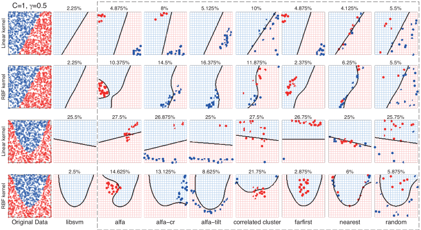
Figure 1: Results on synthetic datasets, for SVMs with the linear (first and third row) and the RBF (second and fourth row) kernel, trained with $C=1$ and $\gamma=0.5$. The original data distribution is shown in the first column (first and second row for the linearly-separable data, third and fourth row for the parabolically-separable data). The decision boundaries of SVMs trained in the absence of label flips, and the corresponding test errors are shown in the second column. The remaining columns report the results for each of the seven considered attack strategies, highlighting the corresponding $L=20$ label flips (out of 200 training samples).

To intuitively understand the fundamental strategies and differences of each of the proposed adversarial label flip attacks, we report here an experimental evaluation on two bi-dimensional datasets, where the positive and the negative samples can be perfectly separated by a linear and a parabolic decision boundary, respectively. For these experiments, we learn SVMs with the linear and the RBF kernel on both datasets, using LibSVM [41]. We set the regularization parameter $C=1$, and the kernel parameter $\gamma=0.5$, based on some preliminary experiments. For each dataset, we randomly select $200$ training samples, and evaluate the test error on a disjoint set of $800$ samples. The proposed attacks are used to flip $L=20$ labels in the training data (i.e., a fraction of 10%), and the SVM model is subsequently learned on the tainted training set. Besides the four proposed attack strategies for adversarial label noise, further three attack strategies are evaluated for comparison, respectively referred to as farfirst, nearest, and random. As for farfirst and nearest, only the labels of the $L$ farthest and of the $L$ nearest samples to the decision boundary are respectively flipped. As for the random attack, $L$ training labels are randomly flipped. To mitigate the effect of randomization, each random attack selects the best label flips over $10$ repetitions.

Results are reported in Fig. 1. First, note how the proposed attack strategies alfa, alfa-cr, alfa-tilt, and correlated cluster generally exhibit clearer patterns of flipped labels than those shown by farfirst, nearest, and random, yielding indeed higher error rates. In particular, when the RBF kernel is used, the SVM’s performance is significantly affected by a careful selection of training label flips (cf. the error rates between the plots in the first and those in the second row of Fig. 1). This somehow contradicts the result in [30], where the use of bounded kernels has been advocated to improve robustness of SVMs against training data perturbations. The reason is that, in this case, the attacker does not have the ability to make unconstrained modifications to the feature values of some training samples, but can only flip a maximum of $L$ labels. As a result, bounding the feature space through the use of bounded kernels to counter label flip attacks is not helpful here. Furthermore, the security of SVMs may be even worsened by using a non-linear kernel, as it may be easier to significantly change (e.g., “bend”) a non-linear decision boundary using carefully-crafted label flips, thus leading to higher error rates. Amongst the attacks, correlated cluster shows the highest error rates when the linear (RBF) kernel is applied to the linearly-separable (parabolically-separable) data. In particular, when the RBF kernel is used on the parabolically-separable data, even only $10\%$ of label flips cause the test error to increase from $2.5\%$ to $21.75\%$. Note also that alfa-cr and alfa-tilt outperform alfa on the linearly-separable dataset, but not on the parabolically-separable data. Finally, it is worth pointing out that applying the linear kernel on the parabolically-separable data, in this case, already leads to high error rates, making thus difficult for the label flip attacks to further increase the test error (cf. the plots in the third row of Fig. 1).

4.2 On Real-World Datasets

We report now a more systematic and quantitative assessment of our label flip attacks against SVMs, considering five real-world datasets publicly available at the LibSVM website. In these experiments, we aim at evaluating how the performance of SVMs decreases against an increasing fraction of adversarially flipped training labels, for each of the proposed attacks. This will indeed allow us to assess their effectiveness as well as the security of SVMs against adversarial label noise. For a fair comparison, we randomly selected $500$ samples from each dataset, and select the SVM parameters from $C\in\{2^{-7},2^{-6},\ldots,2^{10}\}$ and $\gamma\in\{2^{-7},2^{-6},\ldots,2^{5}\}$ by a $5$-fold cross validation procedure. The characteristics of the datasets used, along with the optimal values of $C$ and $\gamma$ as discussed above, are reported in Table 1. We then evaluate our attacks on a separate test set of $500$ samples, using 5-fold cross validation. The corresponding average error rates are reported in Fig. 2, against an increasing fraction of label flips, for each considered attack strategy, and for SVMs trained with the linear and the RBF kernel.

Characteristics of the real-world datasets
Name	Feature set size	SVM parameters
dna	$124$	Linear kernel $C=0.0078$
		RBF kernel $C=1,\gamma=0.0078$
acoustic	$51$	Linear kernel $C=0.016$
		RBF kernel $C=8,\gamma=0.062$
ijcnn1	$23$	Linear kernel $C=4$
		RBF kernel $C=64,\gamma=0.12$
seismic	$51$	Linear kernel $C=4$
		RBF kernel $C=8,\gamma=0.25$
splice	$60$	Linear kernel $C=0.062$
		RBF kernel $C=4,\gamma=0.062$

Table 1: Feature set sizes and SVM parameters for the real-world datasets.

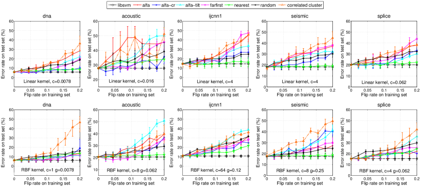
Figure 2: Results on real-world datasets (in different columns), for SVMs with the linear (first row) and the RBF (second row) kernel. Each plot shows the average error rate ($\pm$ half standard deviation, for readability) for each attack strategy, estimated from $500$ samples using 5-fold cross validation, against an increasing fraction of adversarially flipped labels. The values of $C$ and $\gamma$ used to learn the SVMs are also reported for completeness (cf. Table 1).

The reported results show how the classification performance is degraded by the considered attacks, against an increasing percentage of adversarial label flips. Among the considered attacks, correlated cluster shows an outstanding capability of subverting SVMs, although requiring significantly increased computational time. In particular, this attack is able to induce a test error of almost $50\%$ on the dna and seismic data, when the RBF kernel is used. Nevertheless, alfa and alfa-tilt can achieve similar results on the acoustic and ijcnn1 data, while being much more computationally efficient. In general, all the proposed attacks show a similar behavior for both linear and RBF kernels, and lead to higher error rates on most of the considered real-world datasets than the trivial attack strategies farfirst, nearest, and random. For instance, when $20\%$ of the labels are flipped, correlated cluster, alfa, alfa-cr, and alfa-tilt almost achieve an error rate of $50\%$, while farfirst, nearest and random hardly achieve an error rate of $30\%$. It is nevertheless worth remarking that farfirst performs rather well against linear SVMs, while being not very effective when the RBF kernel is used. This reasonably means that non-linear SVMs may not be generally affected by label flips that are far from the decision boundary.

To summarize, our results demonstrate that SVMs can be significantly affected by the presence of well-crafted, adversarial label flips in the training data, which can thus be considered a relevant and practical security threat in application domains where attackers can tamper with the training data.

5 Conclusions and Future Work

Although (stochastic) label noise has been well studied especially in the machine learning literature (e.g., see [32] for a survey), to our knowledge few have investigated the robustness of learning algorithms against well-crafted, malicious label noise attacks. In this work, we have focused on the problem of learning with label noise from an adversarial perspective, extending our previous work on the same topic [34, 35]. In particular, we have discussed a framework that encompasses different label noise attack strategies, revised our two previously-proposed label flip attacks accordingly, and presented two novel attack strategies that can significantly worsen the SVM’s classification performance on untainted test data, even if only a small fraction of the training labels are manipulated by the attacker.

An interesting future extension of this work may be to consider adversarial label noise attacks in which the attacker has limited knowledge of the system, e.g., when the feature set or the training data are not completely known to the attacker, to see whether the resulting error remains considerable also in more practical attack scenarios. Another limitation that may be easily overcome in the future is the assumption of equal cost for each label flip. In general, indeed, a different cost can be incurred depending on the feature values of the considered sample.

We nevertheless believe that this work provides an interesting starting point for future investigations on this topic, and may serve as a foundation for designing and testing SVM-based learning algorithms to be more robust against a deliberate label noise injection. To this end, inspiration can be taken from previous work on robust SVMs to stochastic label noise [45, 34]. Alternatively, one may exploit our framework to simulate a zero-sum game between the attacker and the classifier, that respectively aim to maximize and minimize the classification error on the untainted test set. This essentially amounts to re-training the classifier on the tainted data, having knowledge of which labels might have been flipped, to learn a more secure classifier. Different game formulations can also be exploited if the players use non-antagonistic objective functions, as in [22].

We finally argue that our work may also provide useful insights for developing novel techniques in machine learning areas which are not strictly related to adversarial learning, such as semi-supervised and active learning. In the former case, by turning the maximization in Problems (5)-(6) into a minimization problem, one may find suitable label assignments $\mathbf{z}$ for the unlabeled data, thus effectively designing a semi-supervised learning algorithm. Further, by exploiting the continuous label relaxation of Sect. 3.2, one can naturally implement a fuzzy approach, mitigating the influence of potentially outlying instances. As for active learning, minimizing the objective of Problems (5)-(6) may help identifying the training labels which may have a higher impact on classifier training, i.e., some of the most informative ones to be queried. Finally, we conjecture that our approach may also be applied in the area of structured output prediction, in which semi-supervised and active learning can help solving the inference problem of finding the best structured output prediction approximately, when the computational complexity of that problem is not otherwise tractable.

Huang Xiao got his B.Sc. degree in Computer Science from the Tongji University in Shanghai in China. After that, he got the M.Sc. degree in Computer Science from the Technical University of Munich (TUM) in Germany. His research interests include semi-supervised and nonparametric learning, machine learning in anomaly detection, adversarial learning, causal inference, Bayesian network, Copula theory. He is now a 3rd year PhD candidate at the Dept. of Information Security at TUM, supervised by Prof. Dr. Claudia Eckert.

Battista Biggio received the M. Sc. degree in Electronic Eng., with honors, and the Ph. D. in Electronic Eng. and Computer Science, respectively in 2006 and 2010, from the University of Cagliari, Italy. Since 2007 he has been working for the Dept. of Electrical and Electronic Eng. of the same University, where he is now a postdoctoral researcher. In 2011, he visited the University of Tübingen, Germany, for six months, and worked on the security of machine learning algorithms to training data contamination. His research interests currently include: secure / robust machine learning and pattern recognition methods, multiple classifier systems, kernel methods, biometric authentication, spam filtering, and computer security. He serves as a reviewer for several international conferences and journals, including Pattern Recognition and Pattern Recognition Letters. Dr. Biggio is a member of the IEEE Computer Society and IEEE Systems, Man and Cybernetics Society, and of the Italian Group of Italian Researchers in Pattern Recognition (GIRPR), affiliated to the International Association for Pattern Recognition.

Blaine Nelson is currently a postdoctoral researcher at the University of Cagliari, Italy. He previously was a postdoctoral research fellow at the University of Potsdam and at the University of Tübingen, Germany, and completed his doctoral studies at the University of California, Berkeley. Blaine was a co-chair of the 2012 and 2013 AISec workshops on artificial intelligence and security and was a co-organizer of the Dagstuhl Workshop “Machine Learning Methods for Computer Security” in 2012. His research focuses on learning algorithms particularly in the context of security-sensitive application domains. Dr. Nelson investigates the vulnerability of learning to security threats and how to mitigate them with resilient learning techniques.

Han Xiao is a Ph.D. candidate at Technical University of Munich (TUM), Germany. He got the M.Sc. degree at TUM in 2011. His advisors are Claudia Eckert and René Brandenberg. His research interests include online learning, semi-supervised learning, active learning, Gaussian process, support vector machines and probabilistic graphical models, as well as their applications in knowledge discovery. He is supervised by Claudia Eckert and René Brandenberg. From Sept. 2013 to Jan. 2014, he was a visiting scholar in Shou-De Lin’s Machine Discovery and Social Network Mining Lab at National Taiwan University.

Claudia Eckert got her diploma in computer science from the University of Bonn. And she got the PhD in 1993 and in 1999 she completed her habilitation at the TU Munich on the topic “Security in Distributed Systems”. Her research and teaching activities can be found in the fields of operating systems, middleware, communication networks and information security. In 2008, she founded the center in Darmstadt CASED (Center for Advanced Security Research Darmstadt), she was the deputy director until 2010. She is a member of several scientific advisory boards, including the Board of the German Research Network (DFN), OFFIS, Bitkom and the scientific committee of the Einstein Foundation Berlin. She also advises government departments and the public sector at national and international levels in the development of research strategies and the implementation of security concepts. Since 2013, she is the member of the bavarian academy of science.

Fabio Roli received his M. Sc. degree, with honors, and Ph. D. degree in Electronic Eng. from the University of Genoa, Italy. He was a member of the research group on Image Processing and Understanding of the University of Genoa, Italy, from 1988 to 1994. He was adjunct professor at the University of Trento, Italy, in 1993 and 1994. In 1995, he joined the Dept. of Electrical and Electronic Eng. of the University of Cagliari, Italy, where he is now professor of computer engineering and head of the research group on pattern recognition and applications. His research activity is focused on the design of pattern recognition systems and their applications to biometric personal identification, multimedia text categorization, and computer security. On these topics, he has published more than two hundred papers at conferences and on journals. He was a very active organizer of international conferences and workshops, and established the popular workshop series on multiple classifier systems. Dr. Roli is a member of the governing boards of the International Association for Pattern Recognition and of the IEEE Systems, Man and Cybernetics Society. He is Fellow of the IEEE, and Fellow of the International Association for Pattern Recognition.

References

- Barreno et al. [2006] M. Barreno, B. Nelson, R. Sears, A. D. Joseph, J. D. Tygar, Can machine learning be secure?, in: ASIACCS ’06: Proc. of the ACM Symp. on Inform., Computer and Comm. Sec., ACM, NY, USA, 2006, pp. 16–25.
- Barreno et al. [2010] M. Barreno, B. Nelson, A. Joseph, J. Tygar, The security of machine learning, Machine Learning 81 (2010) 121–148.
- Huang et al. [2011] L. Huang, A. D. Joseph, B. Nelson, B. Rubinstein, J. D. Tygar, Adversarial machine learning, in: 4th ACM Workshop on Artificial Intell. and Security, Chicago, IL, USA, 2011, pp. 43–57.
- Biggio et al. [2014] B. Biggio, G. Fumera, F. Roli, Security evaluation of pattern classifiers under attack, IEEE Trans. on Knowl. and Data Eng. 26 (2014) 984–996.
- Nelson et al. [2008] B. Nelson, M. Barreno, F. J. Chi, A. D. Joseph, B. I. P. Rubinstein, U. Saini, C. Sutton, J. D. Tygar, K. Xia, Exploiting machine learning to subvert your spam filter, in: 1st Usenix Workshop on Large-Scale Exploits and Emergent Threats, USENIX Assoc., CA, USA, 2008, pp. 1–9.
- Nelson et al. [2009] B. Nelson, M. Barreno, F. Jack Chi, A. D. Joseph, B. I. P. Rubinstein, U. Saini, C. Sutton, J. D. Tygar, K. Xia, Misleading learners: Co-opting your spam filter, in: Machine Learning in Cyber Trust, Springer US, 2009, pp. 17–51.
- Rubinstein et al. [2009] B. I. Rubinstein, B. Nelson, L. Huang, A. D. Joseph, S.-h. Lau, S. Rao, N. Taft, J. D. Tygar, Antidote: Understanding and defending against poisoning of anomaly detectors, in: 9th ACM SIGCOMM Internet Measurement Conf., IMC ’09, ACM, New York, NY, USA, 2009, pp. 1–14.
- Biggio et al. [2012] B. Biggio, G. Fumera, F. Roli, L. Didaci, Poisoning adaptive biometric systems, in: G. Gimel’farb, E. Hancock, A. Imiya, A. Kuijper, M. Kudo, S. Omachi, T. Windeatt, K. Yamada (Eds.), Structural, Syntactic, and Statistical Pattern Recognition, volume 7626 of LNCS, Springer Berlin Heidelberg, 2012, pp. 417–425.
- Biggio et al. [2013] B. Biggio, L. Didaci, G. Fumera, F. Roli, Poisoning attacks to compromise face templates, in: 6th IAPR Int’l Conf. on Biometrics, Madrid, Spain, 2013, pp. 1–7.
- Kloft and Laskov [2010] M. Kloft, P. Laskov, Online anomaly detection under adversarial impact, in: 13th Int’l Conf. on Artificial Intell. and Statistics, 2010, pp. 405–412.
- Kloft and Laskov [2012] M. Kloft, P. Laskov, Security analysis of online centroid anomaly detection, J. Mach. Learn. Res. 13 (2012) 3647–3690.
- Biggio et al. [2012] B. Biggio, B. Nelson, P. Laskov, Poisoning attacks against support vector machines, in: J. Langford, J. Pineau (Eds.), 29th Int’l Conf. on Machine Learning, Omnipress, 2012.
- Biggio et al. [2014] B. Biggio, I. Corona, B. Nelson, B. Rubinstein, D. Maiorca, G. Fumera, G. Giacinto, F. Roli, Security evaluation of support vector machines in adversarial environments, in: Y. Ma, G. Guo (Eds.), Support Vector Machines Applications, Springer Int’l Publishing, 2014, pp. 105–153.
- Biggio et al. [2013] B. Biggio, I. Corona, D. Maiorca, B. Nelson, N. Šrndić, P. Laskov, G. Giacinto, F. Roli, Evasion attacks against machine learning at test time, in: H. Blockeel, K. Kersting, S. Nijssen, F. Železný (Eds.), European Conf. on Machine Learning and Principles and Practice of Knowledge Discovery in Databases (ECML PKDD), Part III, volume 8190 of LNCS, Springer Berlin Heidelberg, 2013, pp. 387–402.
- Dalvi et al. [2004] N. Dalvi, P. Domingos, Mausam, S. Sanghai, D. Verma, Adversarial classification, in: 10th ACM SIGKDD Int’l Conf. on Knowledge Discovery and Data Mining, Seattle, 2004, pp. 99–108.
- Lowd and Meek [2005] D. Lowd, C. Meek, Adversarial learning, in: A. Press (Ed.), Proc. of the Eleventh ACM SIGKDD Int’l Conf. on Knowledge Discovery and Data Mining (KDD), Chicago, IL., 2005, pp. 641–647.
- Nelson et al. [2012] B. Nelson, B. I. Rubinstein, L. Huang, A. D. Joseph, S. J. Lee, S. Rao, J. D. Tygar, Query strategies for evading convex-inducing classifiers, J. Mach. Learn. Res. 13 (2012) 1293–1332.
- Biggio et al. [2013] B. Biggio, I. Pillai, S. R. Bulò, D. Ariu, M. Pelillo, F. Roli, Is data clustering in adversarial settings secure?, in: Proc. of the 2013 ACM Workshop on Artificial Intell. and Security, ACM, NY, USA, 2013, pp. 87–98.
- Biggio et al. [ress] B. Biggio, S. R. Bulò, I. Pillai, M. Mura, E. Z. Mequanint, M. Pelillo, F. Roli, Poisoning complete-linkage hierarchical clustering, in: Structural, Syntactic, and Statistical Pattern Recognition, 2014, In press.
- Globerson and Roweis [2006] A. Globerson, S. T. Roweis, Nightmare at test time: robust learning by feature deletion, in: W. W. Cohen, A. Moore (Eds.), Proc. of the 23rd Int’l Conf. on Machine Learning, volume 148, ACM, 2006, pp. 353–360.
- Teo et al. [2008] C. H. Teo, A. Globerson, S. Roweis, A. Smola, Convex learning with invariances, in: J. Platt, D. Koller, Y. Singer, S. Roweis (Eds.), NIPS 20, MIT Press, Cambridge, MA, 2008, pp. 1489–1496.
- Brückner et al. [2012] M. Brückner, C. Kanzow, T. Scheffer, Static prediction games for adversarial learning problems, J. Mach. Learn. Res. 13 (2012) 2617–2654.
- Biggio et al. [2011] B. Biggio, G. Fumera, F. Roli, Design of robust classifiers for adversarial environments, in: IEEE Int’l Conf. on Systems, Man, and Cybernetics, 2011, pp. 977–982.
- Rodrigues et al. [2009] R. N. Rodrigues, L. L. Ling, V. Govindaraju, Robustness of multimodal biometric fusion methods against spoof attacks, J. Vis. Lang. Comput. 20 (2009) 169–179.
- Kolcz and Teo [2009] A. Kolcz, C. H. Teo, Feature weighting for improved classifier robustness, in: 6th Conf. on Email and Anti-Spam, Mountain View, CA, USA, 2009.
- Biggio et al. [2010a] B. Biggio, G. Fumera, F. Roli, Multiple classifier systems under attack, in: N. E. Gayar, J. Kittler, F. Roli (Eds.), 9th Int’l Workshop on Multiple Classifier Systems, volume 5997 of LNCS, Springer, 2010a, pp. 74–83.
- Biggio et al. [2010b] B. Biggio, G. Fumera, F. Roli, Multiple classifier systems for robust classifier design in adversarial environments, Int’l Journal of Machine Learning and Cybernetics 1 (2010b) 27–41.
- Cretu et al. [2008] G. F. Cretu, A. Stavrou, M. E. Locasto, S. J. Stolfo, A. D. Keromytis, Casting out demons: Sanitizing training data for anomaly sensors, in: IEEE Symposium on Security and Privacy, IEEE Computer Society, Los Alamitos, CA, USA, 2008, pp. 81–95.
- Biggio et al. [2011] B. Biggio, I. Corona, G. Fumera, G. Giacinto, F. Roli, Bagging classifiers for fighting poisoning attacks in adversarial environments, in: C. Sansone, J. Kittler, F. Roli (Eds.), 10th Int’l Workshop on Multiple Classifier Systems, volume 6713 of LNCS, Springer-Verlag, 2011, pp. 350–359.
- Christmann and Steinwart [2004] A. Christmann, I. Steinwart, On robust properties of convex risk minimization methods for pattern recognition, J. Mach. Learn. Res. 5 (2004) 1007–1034.
- Kearns and Li [1993] M. Kearns, M. Li, Learning in the presence of malicious errors, SIAM J. Comput. 22 (1993) 807–837.
- Frenay and Verleysen [2013] B. Frenay, M. Verleysen, Classification in the presence of label noise: a survey, IEEE Trans. on Neural Netw. and Learn. Systems PP (2013) 1–1.
- Bshouty et al. [1999] N. Bshouty, N. Eiron, E. Kushilevitz, Pac learning with nasty noise, in: O. Watanabe, T. Yokomori (Eds.), Algorithmic Learning Theory, volume 1720 of LNCS, Springer Berlin Heidelberg, 1999, pp. 206–218.
- Biggio et al. [2011] B. Biggio, B. Nelson, P. Laskov, Support vector machines under adversarial label noise, in: J. Mach. Learn. Res. - Proc. 3rd Asian Conf. Machine Learning, volume 20, 2011, pp. 97–112.
- Xiao et al. [2012] H. Xiao, H. Xiao, C. Eckert, Adversarial label flips attack on support vector machines, in: 20th European Conf. on Artificial Intelligence, 2012.
- Smutz and Stavrou [2012] C. Smutz, A. Stavrou, Malicious pdf detection using metadata and structural features, in: Proc. of the 28th Annual Computer Security Applications Conf., ACSAC ’12, ACM, New York, NY, USA, 2012, pp. 239–248.
- Wang et al. [2014] G. Wang, T. Wang, H. Zheng, B. Y. Zhao, Man vs. machine: Practical adversarial detection of malicious crowdsourcing workers, in: 23rd USENIX Security Symposium, USENIX Association, CA, 2014.
- Cauwenberghs and Poggio [2000] G. Cauwenberghs, T. Poggio, Incremental and decremental support vector machine learning, in: T. K. Leen, T. G. Dietterich, V. Tresp (Eds.), NIPS, MIT Press, 2000, pp. 409–415.
- Diehl and Cauwenberghs [2003] C. P. Diehl, G. Cauwenberghs, SVM incremental learning, adaptation and optimization, in: Int’l J. Conf. on Neural Networks, 2003, pp. 2685–2690.
- Vapnik [1995] V. N. Vapnik, The nature of statistical learning theory, Springer-Verlag New York, Inc., New York, NY, USA, 1995.
- Chang and Lin [2001] C.-C. Chang, C.-J. Lin, LibSVM: a library for support vector machines, 2001. URL: http://www.csie.ntu.edu.tw/~cjlin/libsvm/.
- Lütkepohl [1996] H. Lütkepohl, Handbook of matrices, John Wiley & Sons, 1996.
- Scheinberg [2006] K. Scheinberg, An efficient implementation of an active set method for svms, J. Mach. Learn. Res. 7 (2006) 2237–2257.
- Nelson et al. [2011] B. Nelson, B. Biggio, P. Laskov, Understanding the risk factors of learning in adversarial environments, in: 4th ACM Workshop on Artificial Intell. and Security, AISec ’11, Chicago, IL, USA, 2011, pp. 87–92.
- Stempfel and Ralaivola [2009] G. Stempfel, L. Ralaivola, Learning svms from sloppily labeled data, in: Proc. of the 19th Int’l Conf. on Artificial Neural Networks: Part I, ICANN ’09, Springer-Verlag, Berlin, Heidelberg, 2009, pp. 884–893.