New extraction of CP violation in b-baryon decays

Abstract

We study CP violation in b-baryon decays of $\Xi_{b}^{-}\to\Xi^{-}D$ with $D=D^{0},\bar{D}^{0}$ and $D_{i}~{}(i=1,2)$. We find that these baryonic decay processes provide an ideal opportunity to measure the weak phase due to the absence of the relative strong phase. Explicitly, we relate $\bar{\rho}$ and $\bar{\eta}$ the CKM elements with the decay rate ratios of $R_{i}=\Gamma(\Xi_{b}^{-}\to\Xi^{-}D_{i})/\Gamma(\Xi_{b}^{-}\to\Xi^{-}D^{0})$ without the charge conjugate states. As a complementary, we also examine the decay distributions of $\Lambda_{b}\to\Lambda(\to p\pi^{-})D$. There are in total 32 decay observables, which can be parameterized by 9 real parameters, allowing the experiments to extract the angle $\gamma\equiv\arg(-V_{ud}V_{ub}^{*}/V_{cd}V_{cb}^{*})$ in the CKM unitarity triangle. In addition, the feasibilities of the experimental measurements are discussed. We find that $\bar{\rho}$ and $\bar{\eta}$ can be extracted at LHCb Run3 from $\Xi_{b}^{-}\to\Xi^{-}D$, and a full analysis of $\Lambda_{b}\to\Lambda(\to p\pi^{-})D$ is available at LHCb Run4.

I Introduction

To complete the understanding of the standard model (SM), one of the important tasks is to measure the Cabibbo-Kobayashi-Maskawa (CKM) quark mixing matrix elements. So far, the experimental value of $\gamma\equiv\arg(-V_{ud}V_{ub}^{*}/V_{cd}V_{cb}^{*})$ in the CKM unitarity triangle comes exclusively from the $B$ meson decays LHCb:2017hkl , utilizing the $D^{0}-\overline{D}^{0}$ mixing. The simplest ways are the methods Gronau:1990ra ; Atwood:1996ci of using the $D$ meson two-body sequential decays for CP and flavor taggings. However, their sensitivities are limited by the smallness of the two-body decay branching ratios. To reduce the statistical uncertainties, one can analyze the Dalitz plot in the $D$ meson multibody decays for the two tagging methods Grossman:2002aq . Currently, the most precise value of $\gamma$ is $\left(65.6_{-2.7}^{+0.9}\right)^{\circ}$ and $(65.8\pm 2.2)^{\circ}$ from the CKMfitter CKM and UTfit UT , respectively.

On the other hand, the experimental interests on the b-baryon decays have been increasing rapidly. The evidences of CP violation have been found in various multibody decays LBCP , while the decay width of $\Lambda_{b}\to\Lambda_{c}^{+}\tau^{-}\overline{\nu}_{\tau}$ has been measured for the first time LHCb:2022piu . Besides the branching ratios, the polarizations of the baryons provide fruitful observables in the experiments. In addition, the forward-backward asymmetry of $\Lambda_{b}\to\Lambda\mu^{+}\mu^{-}$ has been studied at LHCb Lambdamu . Notably, the polarization asymmetry of $\Lambda$ in $\Lambda_{b}\to\Lambda\gamma$ has been measured at LHCb for the first time LHCb:2021byf . Recently, a complete analysis of $\Lambda_{b}\to\Lambda(\to p\pi^{-})J/\psi(\to\mu^{+}\mu^{-})$ has been performed Jpsi , where the polarization fraction is found to be around $3\%$ at the centre-of-mass energy of $13$ TeV in $pp$ collisions. Despite these progresses, measurements on the decays associated with a neutral $D$ meson are still lacking.

On the theoretical aspect, the spin nature of the baryons is a double-edge sword, as it provides fruitful phenomenons Observables ; sizable ; TV , but increases the complexity of the quantitative studies. Most of the theoretical studies are performed by the factorization ansatz, within which the color-allowed decays can be estimated reliably Theor ; Zhu:2018jet ; Geng:2020ofy . However, for the color-suppressed decays, one often has to introduce an effective color number by hand to explain the experiments. Fortunately, with the helicity formalism, we can analyze the kinematical systems without knowing the dynamical details Gutsche:2013oea .

The extraction of $\gamma$ via $\Lambda_{b}\to\Lambda D$ with $D=D^{0},\overline{D}^{0},D_{1,2}$ has been given in Refs. Giri:2001ju ; Zhang:2021sit . However, a systematic study of the sequential decays is still missing. In this work, we would use the helicity formalism to explore the sequential modes in the b-baryon decays. In contrast to the orbital angular momentum analysis, the helicity formalism is perfectly compatible with special relativity, and it allows us to extract the information about the baryon spin in a systematic way Jpsi . The difference between the orbital angular momentum and the helicity approaches is discussed in Appendix A.

As mentioned, the extraction of $\gamma$ comes exclusively from $B$ meson decays, and the motivations to extend it to baryon sectors are twofolds. On the theoretical aspect, it is important to study CP violation in baryons, since the matter-antimatter asymmetry in our universe is directly related to them, which can not be explained in the SM. On the experimental aspect, as baryons carry a spin quantum number, it provides us fruitful observables, allowing us to probe the SM further. For instance, the time-reversal violating observables can be constructed even for two-body baryonic decays. In our present work, we concentrate on $\Xi_{b}$ and $\Lambda_{b}$ decays. As mentioned previously, a lot of observations of $\Lambda_{b}$ have been made at LHCb, and after the upgrade, there will also be enough $\Xi_{b}$ to be created. This opens a new window to reexamine $\gamma$ obtained from the meson sectors. We propose to extract $\gamma$ from baryon sectors, by the means of measuring $\Lambda_{b}\to\Lambda D,~{}\Xi_{b}\to\Xi D$ and their sequential decays.

This paper is organized as the follows. In Sec. II, we present the formalism related to the possible physical observables. In Sec. III, we show the numerical results based on the factorization ansatz. We also explore the experimental feasibilities for our results. We conclude the study in Sec. IV.

II Formalism

We analyze the decays of ${\bf B}_{b}\to{\bf B}_{n}D$ with the helicity amplitudes defined by

$$H^{\lambda}_{j}\equiv\langle{\bf B}_{n}D_{j},p\hat{z},\lambda|{\cal H}_{eff}|{\bf B}_{b},J_{z}=\lambda\rangle\,,$$ (1)

where ${\bf B}_{n(b)}=\Lambda_{(b)}$ and $\Xi^{0,-}_{(b)}$ , $\lambda$ and $p\hat{z}$ are the helicity and 3-momentum of ${\bf B}_{n}$, respectively, $j=0,\overline{0},1,2$ denote the $D$ mesons, and $J_{z}$ is the $z$ component of the angular momentum. The derivation and physical meaning of the helicity amplitudes are sketched in Appendix A. In general, the positive helicity amplitudes have the ratios

$$H_{0}^{+}:H_{\overline{0}}^{+}:H_{1}^{+}:H_{2}^{+}=\sqrt{2}:\sqrt{2}r^{+}V:1+r^{+}V:1-r^{+}V\,,$$ (2)

where $r^{+}$ is defined by Eq. (2) itself, and $V$ corresponds to the ratio of the CKM elements, given by $V=V_{ud}V_{ub}^{*}/V_{cd}V_{cb}^{*}=|V|e^{-i\gamma}$ with $V_{qq^{\prime}}$ and $\gamma$ being the CKM elements and unitarity triangle, respectively. The ratios of the negative helicity ones can be obtained by substituting “$-$” for ”$+$” in the superscripts. The amplitudes are related to the CP conjugates as

$$H_{0}^{+}=-\overline{H}_{\overline{0}}^{-}\,,~{}~{}~{}H_{0}^{-}=-\overline{H}_{\overline{0}}^{+}\,,$$ (3)

where we have taken $V_{cd}V_{cb}^{*}$ to be real. The helicities flip signs due to the space inversion, and the minus signs are attributed to the parity of the $D$ mesons.

The amplitude ratios among the charge conjugates are

$$\overline{H}_{0}^{-}:\overline{H}_{\overline{0}}^{-}:\overline{H}_{1}^{-}:\overline{H}_{2}^{-}=-\sqrt{2}r^{+}V^{*}:-\sqrt{2}:-1-r^{+}V^{*}:1-r^{+}V^{*}\,,$$ (4)

with the positive helicity ones given by interchanging “$\pm$” in the superscripts. Combining Eqs. (2)-(4), the 16 complex amplitudes are parameterized by one real and four complex parameters, given by

$$|H^{+}_{0}|\,,~{}~{}\tilde{H}=\frac{H^{-}_{0}}{H_{0}^{+}}\,,~{}~{}~{}r^{\pm}\,,~{}~{}~{}V\,,$$ (5)

which remarkably simplify the analysis.

The decay widths for ${\bf B}_{b}\to{\bf B}_{n}D_{j}$ are given as

$$\Gamma_{j}=\frac{|\vec{p}|}{16\pi M_{{\bf B}_{b}}}\left(\left|H_{j}^{+}\right|^{2}+\left|H_{j}^{-}\right|^{2}\right)\,,$$ (6)

where $\vec{p}$ is the 3-momentum of the daughter particle, and $M_{{\bf B}_{b}}$ denotes the mass of ${\bf B}_{b}$. The full sequential decays ${\bf B}_{b}\to{\bf B}_{n}(\to{\bf B}_{n}^{\prime}\pi)D_{j}$, where ${\bf B}_{n}^{\prime}=\Lambda(p)$ for ${\bf B}_{b}=\Xi_{b}(\Lambda_{b})$, offer three additional observables in the angular distributions. The derivation is given in Appendix A, and the result is sorted as follows:

where $P_{b}$ is the polarized fraction of ${\bf B}_{b}$, depending on its production, and the definitions of the angles are shown in FIG. 1 with $(\theta,\phi)$ and $\theta_{1}$ determined at the rest frames of ${\bf B_{b}}$ and ${\bf B}_{n}$, respectively. In Eq. (II), $\alpha_{n}$ is the up-down asymmetry parameter of ${\bf B}_{n}\to{\bf B}_{n}^{\prime}\pi$, and $\alpha_{j}$, $\beta_{j}$ and $\gamma_{j}$ are given as

$$\alpha_{j}=\frac{1-|\tilde{H}_{j}|^{2}}{1+|\tilde{H}_{j}|^{2}}\,,~{}~{}~{}\beta_{j}=\frac{-2\text{Im}(\tilde{H}_{j})}{1+|\tilde{H}_{j}|^{2}}\,,~{}~{}~{}\gamma_{j}=\frac{2\text{Re}(\tilde{H}_{j})}{1+|\tilde{H}_{j}|^{2}}\,,$$ (7)

respectively, where $\tilde{H}_{j}$ are defined by

$$\tilde{H}_{j}=H_{j}^{-}/H_{j}^{+}\,,$$ (8)

with the explicit parametrizations in Table 1 , $\alpha_{j}$ describe the polarized asymmetries of the daughter baryons, and $\beta_{j}$ represent T violation for the absence of strong phases Geng:2020ofy .

To measure $\alpha_{j}$, $\beta_{j}$ and $\gamma_{j}$, it is convention to recast them in the forms based on the numbers of events, $N$, given as

$$\alpha_{j}=\frac{2}{\alpha_{n}}\frac{N(\hat{p}_{{\bf B}_{n}^{\prime}}\cdot\hat{p}_{D_{j}}<0)-N(\hat{p}_{{\bf B}_{n}^{\prime}}\cdot\hat{p}_{D_{j}}>0)}{N(\hat{p}_{{\bf B}_{n}^{\prime}}\cdot\hat{p}_{D_{j}}>0)+N(\hat{p}_{{\bf B}_{n}^{\prime}}\cdot\hat{p}_{D_{j}}<0)}\,,$$

$$\beta_{j}=\frac{8}{P_{b}\alpha_{n}\pi}\frac{N\left((\hat{p}_{{\bf B}_{n}^{\prime}}\times\hat{p}_{D_{j}})\cdot\hat{n}_{{\bf B}_{b}}>0\right)-N\left((\hat{p}_{{\bf B}_{n}^{\prime}}\times\hat{p}_{D_{j}})\cdot\hat{n}_{{\bf B}_{b}}<0\right)}{N\left((\hat{p}_{{\bf B}_{n}^{\prime}}\times\hat{p}_{D_{j}})\cdot\hat{n}_{{\bf B}_{b}}>0\right)+N\left((\hat{p}_{{\bf B}_{n}^{\prime}}\times\hat{p}_{D_{j}})\cdot\hat{n}_{{\bf B}_{b}}<0\right)}\,,$$ (9)

$$\gamma_{j}=\frac{8}{P_{b}\alpha_{n}\pi}\frac{N\left((\hat{p}_{D_{j}}\times\hat{n}_{{\bf B}_{b}})\cdot(\hat{p}_{D_{j}}\times\hat{p}_{{\bf B}_{n}^{\prime}})>0\right)-N\left((\hat{p}_{D_{j}}\times\hat{n}_{{\bf B}_{b}})\cdot(\hat{p}_{D_{j}}\times\hat{p}_{{\bf B}_{n}^{\prime}})<0\right)}{N\left((\hat{p}_{D_{j}}\times\hat{n}_{{\bf B}_{b}})\cdot(\hat{p}_{D_{j}}\times\hat{p}_{{\bf B}_{n}^{\prime}})>0\right)+N\left((\hat{p}_{D_{j}}\times\hat{n}_{{\bf B}_{b}})\cdot(\hat{p}_{D_{j}}\times\hat{p}_{{\bf B}_{n}^{\prime}})<0\right)}\,,$$

respectively, where the equations hold at the limit of $N\to\infty$.

Table 1: The parameterization of $\tilde{H}_{j}$.

$D$	$\tilde{H}_{j}({{\bf B}_{b}\to{\bf B}_{n}D})$	$\tilde{H}_{j}({\overline{\bf B}}_{b}\to{\overline{\bf B}}_{n}D)$
$D^{0}$	$\tilde{H}$	$\frac{\displaystyle r^{+}}{\displaystyle r^{-}}\tilde{H}^{-1}$
$\overline{D}^{0}$	$\frac{\displaystyle r^{-}}{\displaystyle r^{+}}\tilde{H}$	$\tilde{H}^{-1}$
$D_{1}$	$\frac{\displaystyle 1+r^{+}V}{\displaystyle 1+r^{-}V}\tilde{H}$	$\frac{\displaystyle 1+r^{+}V^{*}}{\displaystyle 1+r^{-}V^{*}}\tilde{H}^{-1}$
$D_{2}$	$\frac{\displaystyle 1-r^{+}V}{\displaystyle 1-r^{-}V}\tilde{H}$	$\frac{\displaystyle 1-r^{+}V^{*}}{\displaystyle 1-r^{-}V^{*}}\tilde{H}^{-1}$

The CP violating asymmetries are constructed as

$$A_{j}^{CP}=\frac{\Gamma_{j}-\overline{\Gamma}_{\overline{j}}}{\Gamma_{j}+\overline{\Gamma}_{\overline{j}}}\,,~{}~{}~{}\Delta\xi_{j}=\frac{1}{2}\left(\xi_{j}+\overline{\xi}_{\overline{j}}\right),~{}~{}~{}\Delta\gamma_{j}=\frac{1}{2}\left(\gamma_{j}-\overline{\gamma}_{\overline{j}}\right)\,,~{}~{}~{}\text{with}~{}\xi_{j}=\alpha_{j},\beta_{j},$$ (15)

where the overlines on $\Gamma_{j}$, $\xi_{j}$ and $\gamma_{j}$ correspond to the charge conjugate ones of the baryons, and $\overline{j}=\overline{0},0,1,2$ for $j=0,\overline{0},1,2$ , respectively. Note that $A^{CP}_{j}$ are the direct CP asymmetries, and the others are the CP violating obeservables in the decay angular distributions.

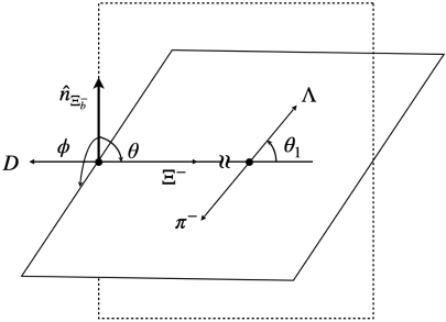
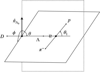
Figure 1: Decay planes for ${\bf B}_{b}\to{\bf B}_{n}(\to{\bf B}_{n}^{\prime}\pi)D$.

To get a clearer view of $\Delta\xi_{j}$ as well as $\Delta\gamma_{j}$, we rewrite the decay parameters as

$$\xi_{j}^{CP}=\Delta\xi_{j}+\frac{1}{2}A_{j}^{CP}\left(\xi_{j}-\overline{\xi}_{\overline{j}}\right)\,,~{}~{}~{}\gamma_{j}^{CP}=\Delta\gamma_{j}+\frac{1}{2}A_{j}^{CP}\left(\gamma_{j}+\overline{\gamma}_{\overline{j}}\right)\,,$$ (16)

with

$$\xi_{j}^{CP}=\frac{{\xi_{j}\Gamma_{j}+\overline{\xi}_{\overline{j}}\overline{\Gamma}_{\overline{j}}}}{\Gamma_{j}+\overline{\Gamma}_{\overline{j}}}\,,~{}~{}~{}\gamma_{j}^{CP}=\frac{{\gamma_{j}\Gamma_{j}-\overline{\gamma}_{\overline{j}}\overline{\Gamma}_{\overline{j}}}}{\Gamma_{j}+\overline{\Gamma}_{\overline{j}}}\,.$$ (17)

As there is only one weak phase in the decay channels with $D^{0}$ and $\overline{D}^{0}$, we have

$$A_{0}^{CP}=A_{\overline{0}}^{CP}=\xi^{CP}_{0}=\xi^{CP}_{\overline{0}}=\gamma^{CP}_{0}=\gamma_{\overline{0}}^{CP}=0\,,$$ (18)

derived from Eqs. (2)-(4) . The right sides of the two equations in Eq. (16) can be measured from the experiments, whereas the left ones can be written down in compact ways as

$$A_{1,2}^{CP}=\frac{\pm 2{\cal X}_{+}}{\langle H_{1,2}^{2}\rangle}\,,~{}~{}\alpha_{1,2}^{CP}=\frac{\pm 2{\cal X}_{-}}{\langle H_{1,2}^{2}\rangle}\,,~{}~{}\beta_{1,2}^{CP}=\frac{\pm 2\text{Re}({\cal Y})}{\langle H_{1,2}^{2}\rangle}\,,~{}~{}\gamma_{1,2}^{CP}=\frac{\pm 2\text{Im}({\cal Y})}{\langle H_{1,2}^{2}\rangle}\,,$$ (19)

where

$${\cal X}_{\pm}=-\text{Im}(V)\text{Im}\left(r^{+}\pm|\tilde{H}|^{2}r^{-}\right)\,,~{}~{}{\cal Y}=\text{Im}(V)\tilde{H}_{j}\left(r^{+*}-r^{-}\right)\,,$$

$$\langle H_{1,2}^{2}\rangle=1+|\tilde{H}|^{2}\pm 2\text{Re}(r^{+}+r^{-}|\tilde{H}|^{2})\text{Re}(V)+\left(|r^{+}|^{2}+|\tilde{H}r^{-}|^{2}\right)|V|^{2}\,.$$ (20)

It is then straightforward to see that the observables defined in Eq. (15) are CP odd, as they are proportional to Im$(V)$.

It is not a coincidence that the CP violating asymmetries of $D_{1}$ and $D_{2}$ differ minus signs in the numerators of Eq. (19), as can be seen from the following identities:

$$(\Gamma_{1}+\overline{\Gamma}_{1})\xi^{CP}_{1}+(\Gamma_{2}+\overline{\Gamma}_{2})\xi^{CP}_{2}=(\Gamma_{0}+\overline{\Gamma}_{\overline{0}})\xi^{CP}_{0}+(\Gamma_{\overline{0}}+\overline{\Gamma}_{0})\xi^{CP}_{\overline{0}}=0\,,$$

$$(\Gamma_{1}+\overline{\Gamma}_{1})\gamma^{CP}_{1}+(\Gamma_{2}+\overline{\Gamma}_{2})\gamma^{CP}_{2}=(\Gamma_{0}+\overline{\Gamma}_{\overline{0}})\gamma^{CP}_{0}+(\Gamma_{\overline{0}}+\overline{\Gamma}_{0})\gamma^{CP}_{\overline{0}}=0\,.$$ (21)

In Eq. (II), the first equality comes from that the physical quantities are independent of the basis (either flavor or CP), and the second one is due to Eq. (18).

III Numerical Results

To analyze the decays quantitatively, we begin with the effective Hamiltonian Buras:1991jm , given by

$${\cal H}_{eff}=\frac{G_{F}}{\sqrt{2}}\left[V_{cb}V_{us}^{*}\left(C_{1}O^{c}_{1}+C_{2}O^{c}_{2}\right)+V_{ub}V_{cs}^{*}\left(C_{1}O^{u}_{1}+C_{2}O^{u}_{2}\right)\right]+h.c.\,,$$ (22)

with

$$O_{1}^{c}=(\overline{c}_{\beta}u_{\alpha})_{V-A}(\overline{d}_{\alpha}b_{\beta})_{V-A}\,,~{}~{}~{}~{}O_{2}^{c}=(\overline{c}_{\alpha}u_{\alpha})_{V-A}(\overline{d}_{\beta}b_{\beta})_{V-A}\,,$$

$$O_{1}^{u}=(\overline{u}_{\beta}c_{\alpha})_{V-A}(\overline{d}_{\alpha}b_{\beta})_{V-A}\,,~{}~{}~{}~{}O_{2}^{u}=(\overline{u}_{\alpha}c_{\alpha})_{V-A}(\overline{d}_{\beta}b_{\beta})_{V-A}\,,$$ (23)

where $G_{F}$ is the Fermi constant, $C_{1,2}$ are the Wilson coefficients, $\alpha$ and $\beta$ correspond to the color indices, and $h.c.$ represents the Hermitian conjugate. Note that we have used the Fierz transformation to sort the operators.

The quark diagrams of ${\bf B}_{b}\to{\bf B}_{n}D$ are shown in FIG. 2. There is only one possible type of quark diagrams for $\Xi_{b}^{-}\to\Xi^{-}D$ (the left one in FIG. 2). In contrast, the decays of $\Lambda_{b}$ have two extra nonfactorizable diagrams (the middle and right ones in FIG. 2), which would introduce different strong phases and increase the complexity of the analysis. In the following, unless stated otherwise, we concentrate on $\Xi_{b}^{-}\to\Xi^{-}D$.

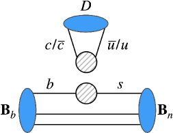
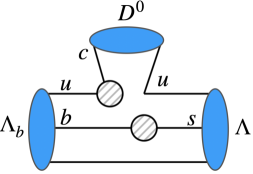
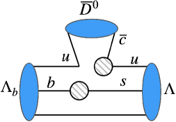
Figure 2: Quark diagrams of the b-baryons decays

The amplitude ratios of $\Xi_{b}^{-}\to\Xi^{-}D$ can be naively read off in a model independent way from FIG. 1. As $\Xi_{b}^{-}\to\Xi^{-}D^{0}$ and $\Xi_{b}^{-}\to\Xi^{-}\overline{D}^{0}$ share the same diagram, they receive the same corrections from the strong interactions. Thus, we deduce that $r^{\pm}=1$ in Eq. (2) for $\Xi_{b}^{-}\to\Xi^{-}D$, leading to

$$\Gamma_{0}:\Gamma_{\overline{0}}:\Gamma_{1}:\Gamma_{2} = 2:2\overline{\rho}^{2}+2\overline{\eta}^{2}:1+2\overline{\rho}+\overline{\rho}^{2}+\overline{\eta}^{2}:1-2\overline{\rho}+\overline{\rho}^{2}+\overline{\eta}^{2}\,,$$ (24)

to ${\cal O}(\lambda^{4})$ precision with $\lambda$, $\overline{\rho}$ and $\overline{\eta}$ the Wolfenstein parameters for the CKM matrix CKM . As the total branching ratios are independent of the basis (flavor or CP), we have

$$\Gamma_{0}+\Gamma_{\overline{0}}=\Gamma_{1}+\Gamma_{2}\,,$$ (25)

which can also be easily seen from Eq. (24) . Hence, there have only two independent ratios along with the two parameters $(\overline{\rho},\overline{\eta})$. Clearly, it is possible to extract both $\overline{\rho}$ and $\overline{\eta}$ from the experiments, given by

$$\overline{\rho}=\frac{1}{2}\left(R_{1}-R_{2}\right)\,,~{}~{}~{}\overline{\eta}=\sqrt{R_{1}+R_{2}-\frac{1}{4}\left(R_{1}-R_{2}\right)^{2}-1}\,,$$ (26)

with $R_{1,2}=\Gamma_{1,2}/\Gamma_{0}$ . Remarkably, the extractions do not require the charge conjugate states. We emphasize that Eqs. (24) and (26) are model independent based on the analysis from the quark diagrams.

To estimate the results in the experiments, we adopt the framework of the naïve factorization. The amplitudes are then read as

$$\frac{G_{F}}{\sqrt{2}}a_{2}V_{cb}V_{us}^{*}\langle D^{0}|(\overline{c}u)_{V-A}|0\rangle\langle\Xi^{-}|(\overline{s}b)_{V-A}|\Xi^{-}_{b}\rangle\,,$$ (27)

where $a_{2}$ is the effective Wilson coefficient for the color-suppressed decays. For the numerical results, we take the large $N_{c}$ limit leading to $a_{2}=c_{2}=-0.365$ Buras:1991jm . The baryon transition matrix elements can be further decomposed as

$$\langle\Xi^{-}|\overline{s}\gamma^{\mu}b|\Xi^{-}_{b}\rangle = \overline{u}\left(f_{1}(M_{D}^{2})\gamma^{\mu}-f_{2}(M_{D}^{2})i\sigma_{\mu\nu}\frac{p_{D}^{\nu}}{M_{\Xi^{-}_{b}}}+f_{3}(M_{D}^{2})\frac{p_{D}^{\mu}}{M_{\Xi^{-}_{b}}}\right)u_{b}\,,$$

$$\langle\Xi^{-}|\overline{s}\gamma^{\mu}\gamma^{5}b|\Xi^{-}_{b}\rangle = \overline{u}\left(g_{1}(M_{D}^{2})\gamma^{\mu}-g_{2}(M_{D}^{2})i\sigma_{\mu\nu}\frac{p_{D}^{\nu}}{M_{\Xi^{-}_{b}}}+g_{3}(M_{D}^{2})\frac{p_{D}^{\mu}}{M_{\Xi^{-}_{b}}}\right)\gamma^{5}u_{b}\,,$$ (28)

where $u_{(b)}$ is the Dirac spinor of $\Xi_{(b)}^{-}$, $M_{D(\Xi_{b}^{-})}$ and $p^{\mu}_{D}$ are the masses and the 4-momentum of $D(\Xi_{b}^{-})$, respectively, and $f_{i}$ and $g_{i}$ are the form factors with $i=1,2$ and $3$. The helicity amplitudes are related to the form factors as

$$H^{\pm}_{0}=Q_{+}A\mp Q_{-}B\,,$$ (29)

where

$$Q_{\pm}=\sqrt{(M_{\Xi^{-}_{b}}\pm M_{\Xi^{-}})^{2}-M_{D}^{2}}$$

$$A=\frac{G_{F}}{\sqrt{2}}a_{2}f_{D}V_{cb}V_{us}^{*}\left[\left(M_{\Xi^{-}_{b}}-M_{\Xi^{-}}\right)f_{1}+\frac{M_{D}^{2}}{M_{\Xi^{-}_{b}}}f_{3}\right]\,,$$

$$B=\frac{G_{F}}{\sqrt{2}}a_{2}f_{D}V_{cb}V_{us}^{*}\left[\left(M_{\Xi^{-}_{b}}+M_{\Xi^{-}}\right)g_{1}-\frac{M_{D}^{2}}{M_{\Xi^{-}_{b}}}g_{3}\right]\,.$$ (30)

The rest of the amplitudes can be obtained by taking $r^{\pm}=1$ in Eq. (2) .

In this work, the form factors are calculated by the homogeneous bag model Geng:2020ofy , in which the center motions of the hadrons are removed by the linear superposition of infinite bags, allowing the form factors to be calculated consistently. Particularly, with the homogeneous bag model, the experimental branching ratios of $\Lambda_{b}\to\Lambda_{c}^{+}\pi^{+}/K^{+}$ and $\Lambda_{b}\to p\pi^{+}/K^{+}$ can be well explained Geng:2020ofy ; sizable . All the model parameters can be extracted from the mass spectra, given as  Zhang:2021yul

$$R=(4.6\pm 0.2)~{}\text{GeV}^{-1}\,,~{}~{}~{}M_{u,d}=0\,,~{}~{}~{}M_{s}=0.28~{}\text{GeV}\,,~{}~{}~{}M_{b}=5.093~{}\text{GeV}\,,$$ (31)

where $R$ is the bag radius. For the detail derivations, the readers are referred to Ref. Geng:2020ofy  .

In Table 2, we list our numerical of the decay widths and observables. At the chiral limit, the emitted $s$ quark due to the weak interaction is essentially left-handed, leading to $\alpha_{j}\approx-1$. As a result, we have that $\beta_{j}=0$ for $\tilde{H}$ being real within the factorization framework. In addition, as there is no relative strong phase, the CP violating effects are absent.

Table 2: Decay widths and observables

Baryon	$D$	$\Gamma/\Gamma_{0}$	$10^{6}{\cal B}$	$\alpha_{j}$	$\gamma^{\prime}_{j}$
$\Xi_{b}^{-}\to\Xi^{-}$	$D^{0}$	$\equiv 1$	$9.7\pm 1.6$	$-0.99\pm 0.01$	$0.06\pm 0.02$
	$D_{1}$	$0.71\pm 0.02$	$6.9\pm 1.2$
	$D_{2}$	$0.43\pm 0.01$	$4.2\pm 0.7$
	$\overline{D^{0}}$	$0.14\pm 0.01$	$1.4\pm 0.3$
$\Lambda_{b}\to\Lambda$	$D^{0}$	$\equiv 1$	$6.6\pm 0.6$	$-0.99\pm 0.01$	$0.06\pm 0.02$
	$D_{1}$	$0.71\pm 0.02$	$4.7\pm 0.5$
	$D_{2}$	$0.43\pm 0.01$	$2.9\pm 0.3$
	$\overline{D^{0}}$	$0.14\pm 0.01$	$0.9\pm 0.1$

The results of $\Lambda_{b}\to\Lambda D$, estimated with the naïve factorization, are also given to compare with those in the literature. Our prediction of ${\cal B}(\Lambda_{b}\to D^{0}\Lambda)$ is roughly 1.2 times larger than the one in Ref. Giri:2001ju and twice larger than that in Ref. Zhu:2018jet . It is attributed to the use of a larger $a_{2}$ in our study. Since $\alpha_{j}$ are independent of $a_{2}$, the predicted values of $\alpha_{j}$ are well consistent with those in Ref. Zhu:2018jet , which are direct consequences from the factorization approach.

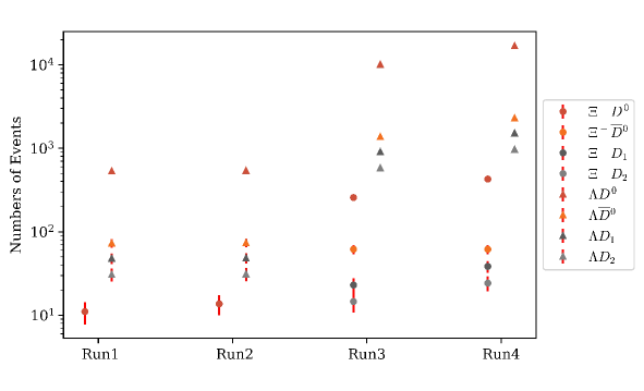
Figure 3: The estimated values of $N(\Lambda_{b}\to\Lambda(\to p\pi^{-})D)$ and $N(\Xi_{b}^{-}\to\Xi^{-}(\to\Lambda\pi)D)$ at LHCb, where the red ones represent the statistical uncertainties.

The possible sequential decays for the flavor and CP taggings are BESIII:2020khq

$$\begin{array}[]{l}D^{0}:K^{-}\pi^{+}\,,~{}K^{-}\pi^{+}\pi^{0}\,,~{}K^{-}\pi^{+}\pi^{+}\pi^{-}\,,~{}K^{-}e^{+}\nu_{e}\,,\\ D_{1}:K_{S}^{0}\pi^{0}\,,K_{S}^{0}\eta\,,K_{S}^{0}\omega\,,K_{S}^{0}\eta^{\prime}\,,\\ D_{2}:K^{+}K^{-}\,,\pi^{+}\pi^{-}\,,K_{S}^{0}\pi^{0}\pi^{0}\,,K_{L}^{0}\pi^{0}\,,\pi^{+}\pi^{-}\pi^{0}\,.\\ \end{array}$$ (44)

By crunching up their branching ratios, the ideal efficiencies are $30\%$ for the flavor tagging and $(3.8,4.0)\%$ for $D_{1,2}$. Accordingly, we give estimations in FIG. 3 through

$$N(\Lambda_{b}\to\Lambda(\to p\pi^{-})D)={\cal N}_{\Lambda_{b}}\times\mathcal{B}(\Lambda_{b}\to\Lambda(\to p\pi^{-})D)\times\epsilon_{\text{Dtag}}\times\epsilon_{\text{exp}},$$

$$N(\Xi_{b}^{-}\to\Xi^{-}(\to\Lambda\pi^{-})D)={\cal N}_{\Xi_{b}^{-}}\times\mathcal{B}(\Xi_{b}\to\Xi^{-}(\to\Lambda\pi^{-})D)\times\epsilon_{\text{Dtag}}\times\epsilon_{\text{exp}},$$ (45)

where $N$ represent the numbers of the observed events, while ${\cal N}_{{\bf B}_{b}}$ are the produced numbers of ${\bf B}_{b}=\Lambda_{b},\Xi_{b}^{-}$, at the experiments. The estimated values of ${\cal N}_{{\bf B}_{b}}$ can be found in Appendix B. Here, $\epsilon_{\text{exp}}$ are taken to be $7.25\%$ and $0.96\%$ for $\Lambda_{b}\to\Lambda(\to p\pi^{-})D$ and $\Xi_{b}\to\Xi(\to p\pi^{-})D$ LHCb:2019sxa , respectively.

From the figure, we have that $N(\Xi_{b}^{-}\to\Xi^{-}(\to\Lambda\pi^{-})D^{0},\overline{D}^{0},D_{1})=(200,50,20)$ at LHCb Run3, which are sufficient for measuring $\overline{\eta}$ and $\overline{\rho}$ via Eq. (26). At LHC Run4, $N(\Lambda_{b}\to\Lambda(\to p\pi^{-})D^{0})$ and $N(\Lambda_{b}\to\Lambda(\to p\pi^{-})D_{1,2})$ would be $2\times 10^{4}$ and $2\times 10^{3}$, respectively, providing enough data points to reconstruct the full angular distributions, and allowing the experiments to extract $\gamma$.

IV Conclusion

We have systematically studied the decays of ${\bf B}_{b}\to{\bf B}_{n}D$, and discussed the feasibilities of the experimental measurements. Remarkably, the process of $\Xi_{b}^{-}\to\Xi^{-}D$ contains only one quark diagram, and therefore provides an ideal place to extract the weak phase. We have shown that the Wolfenstein parameters of the CKM matrix can be extracted by $\overline{\rho}=(R_{1}-R_{2})/2$ and $\overline{\eta}=\sqrt{R_{1}+R_{2}-\frac{1}{4}(R_{1}-R_{2})^{2}-1}$, which are feasible to be measured at LHC Run3.

As the baryons can be polarized, we have demonstrated that the decays of the b-baryons provide much richer observables compared to the mesons. All the possible observables have been parameterized with 9 real parameters, which allows the future experiments to extract the CP violating unitarity angle of $\gamma$ in the CKM matrix. At LHCb Run4 , a complete study of $\Lambda_{b}\to\Lambda(\to p\pi^{-})D$ on the angular distribution has shown to be promising.

On the other hand, to get quantitative results, the decay observables have been studied with the factorization ansatz. In particular, we have found that ${\cal B}(\Xi_{b}^{-}\to\Xi^{-}D)=(9.7\pm 1.6,1.4\pm 0.3,6.9\pm 1.2,4.2\pm 1.7)\times 10^{-6}$ for $D=D^{0},\overline{D}^{0},D_{1},D_{2}$, respectively. We have also estimated the numerical results of $\Lambda_{b}\to\Lambda D$, which are compatible with those in the literature.

Appendix A Angular analysis and helicity formlism

In this appendix, we would like to compare the pros and cons between the traditional approach and the helicity formalism. First, we briefly review the traditional approach toward the angular distribution Pakvasa:1990if .

According to the Lorentz structure, the amplitudes of ${\bf B}_{b}\to{\bf B}_{n}D$ are traditionally parameterized as

$$M=i\overline{u}\left(A-B\gamma_{5}\right){u}_{b}\,,$$ (46)

where $A$ and $B$ are parameters to be determined by theories or experiments. Notice that with Eq. (46), we have chosen the spinor representations for ${\bf B}_{b,n}$. Traditionally, Eq. (46) is recasted as

$$M=\chi_{n}^{\dagger}(S+P\sigma\cdot\mathbf{q})\chi_{b},$$ (47)

with

$$S=i\sqrt{2M_{b}(E_{n}+M_{n})}A\,,~{}~{}~{}~{}~{}P=-i\sqrt{2M_{b}(E_{n}-M_{n})}B$$ (48)

where $\chi_{b(n)}$ is the two-component spinor of ${\bf B}_{b(n)}$, and $\mathbf{q}$ is the unit vector of the ${\bf B}_{n}$’s 3-momentum at the ${\bf B}_{b}$ rest frame. The symbols of $``S^{\prime\prime}$ and $``P^{\prime\prime}$ are related to $L=0$ and $L=1$, respectively, where $L$ stands for the orbital angular momentum. However, it is well known that the orbital angular momentum is ill-defined for massless particles, and thus incompatible to the special relativity.

By squaring the amplitudes and noting

$$\chi_{b}\chi_{b}^{\dagger}=\left(\frac{1}{2}+\frac{1}{2}{\bf s}_{b(n)}\cdot{\sigma}\right)\,,$$ (49)

we arrive

$$1+\alpha_{j}\mathbf{q}\cdot(\mathbf{s}_{b}+\mathbf{s}_{n})+(\mathbf{s}_{b}\cdot\mathbf{q})(\mathbf{s}_{n}\cdot\mathbf{q})+\beta_{j}\mathbf{s}_{b}\times\mathbf{q}\cdot\mathbf{s}_{n}+\gamma_{j}\mathbf{q}\times(\mathbf{s}_{b}\times\mathbf{q})\cdot\mathbf{s}_{n},$$ (50)

where ${\bf s}_{b(n)}$ satisfies

$$\left({\bf s}_{b(n)}\cdot\sigma\right)\chi_{b(n)}=\chi_{b(n)}\,.$$ (51)

Naively, one would tend to interpret ${\bf s}_{b(n)}$ as the spin of ${\bf B}_{b(n)}$. Nonetheless, if we adopt such interpretation, Eq. (50) would force us to commit $({\bf s}_{b,n})_{x}$, $({\bf s}_{b,n})_{y}$ and $({\bf s}_{b,n})_{z}$ commute with each others, as the notation suggests that ${\bf B}_{b,n}$ are the eigenstates of them simultaneously. Although the outcomes might be correct, the interpretation is fatally wrong on the theoretical aspect TV ; sizable . Moreover, in the experiments, spins can not be measured directly, and it is hard to deduce physical observables from Eq. (50).

In comparison, the helicity formalism is outstanding on many aspects. It is perfectly compatible with massless objects, and the angular distributions of sequential decays can be easily deduced. For two-body systems, the eigenstates of helicities and angular momenta are constructed as

$$|\lambda_{1}\,,\lambda_{2},J,J_{z}\rangle=\frac{1}{(2J+1)\pi}\int d\cos\theta d\phi|p,\theta,\phi,\lambda_{1}\,,\lambda_{2}\rangle e^{iJ_{z}\phi}d^{J}(\theta)^{J_{z}}\,_{\lambda_{1}-\lambda_{2}}\,,$$ (52)

with

$$|p,\theta,\phi,\lambda_{1},\lambda_{2}\rangle=R_{z}(\phi)R_{y}(\theta)\left(|f_{1};\vec{p}=p\vec{z},\lambda_{1}\rangle\otimes|f_{2};\vec{p}=-p\vec{z},\lambda_{2}\rangle\right)\,,$$ (53)

where $f_{1,2}$ stand for the first and the second particles with opposite 3-momenta, $\lambda_{1,2}$ are the helicities of $f_{1,2}$, $J$ and $J_{z}$ are the angular momentum and its $z$ component of the systems, respectively, $d$ stands for the Wigner-$d$ matrix, and $R_{y,z}$ are the rotation operators pointing toward $\hat{y}(\hat{z})$.

For the weak decays of $i\to f_{1}f_{2}$, where $i$ is an arbitrary particle pointing toward $\hat{z}$, the angular distributions are given as

$$\frac{\partial^{2}\Gamma}{\partial\phi\partial\cos\theta}\propto\sum_{\lambda_{1},\lambda_{2}}\left|\langle p,\theta,\phi,\lambda_{1},\lambda_{2}|{\cal H}_{eff}|i;J,J_{z}\rangle\right|^{2}\,.$$ (54)

The helicities of the outgoing particles must be summed over as they are not distinguishable in the experiments. By inserting the identity

$$1=\sum_{J,J_{z},\lambda_{1},\lambda_{2}}\frac{4\pi}{2J+1}|J,J_{z},\lambda_{1},\lambda_{2}\rangle\langle J,J_{z},\lambda_{1},\lambda_{2}|\,,$$ (55)

we arrive at

$$\frac{\partial^{2}\Gamma}{\partial\phi\partial\cos\theta}\propto\sum_{\lambda_{1},\lambda_{2}}\left|e^{iJ_{z}\phi}d^{J}(\theta)^{J_{z}}\,_{\lambda_{1}-\lambda_{2}}H^{\lambda_{1}\lambda_{2}}\right|^{2}\,,$$ (56)

with

$$H^{\lambda_{1},\lambda_{2}}\equiv\langle J,J_{z},\lambda_{1},\lambda_{2}|{\cal H}_{eff}|i;J,J_{z}\rangle\,.$$ (57)

Here, $H^{\lambda_{1},\lambda_{2}}$ can not depend on $J_{z}$ as ${\cal H}_{eff}$ is a scalar, and the exponential in Eq. (56) can clearly be omitted. We can see that the amplitudes are now decomposed into two parts; the kinematic part is described by the Wigner-$d$ matrices, while the dynamical one by $H^{\lambda_{1},\lambda_{2}}$. Using the inverse of Eq. (52), given as

$$|p\hat{z},\lambda_{1},\lambda_{2}\rangle=\sum_{J}|J,J_{z}=\lambda_{1}-\lambda_{2},\lambda_{1},\lambda_{2}\rangle\,,$$ (58)

we arrive at

$$H^{\lambda_{1},\lambda_{2}}=\langle p\hat{z},\lambda_{1},\lambda_{2}|{\cal H}_{eff}|i;J,\lambda_{1}-\lambda_{2}\rangle\,,$$ (59)

which is handy in computing the numerical results.

Angular distributions of sequential decays can be obtained by applying the above method multiple times. For ${\bf B}_{b}\to{\bf B}_{n}(\to{\bf B}_{n}^{\prime}\pi)D_{j}$, we have

$${\cal D}_{j}\propto\sum_{\lambda_{n}^{\prime},J_{z}}\rho_{J_{z}J_{z}}\left|\sum_{\lambda_{n}}H^{\lambda_{n}}_{j}H^{\prime\lambda_{n}^{\prime}}e^{i\lambda_{n}\phi}d^{\frac{1}{2}}(\theta)^{J_{z}}\,_{\lambda_{n}}d^{\frac{1}{2}}(\theta_{1})^{\lambda_{n}}\,_{\lambda_{n}^{\prime}}\right|\,,$$ (60)

where $H_{j}^{\lambda_{n}}$ describes the dynamic of ${\bf B}_{b}\to{\bf B}_{n}D_{j}$ and $H^{\lambda_{n}^{\prime}}$ of ${\bf B}_{n}\to{\bf B}_{n}^{\prime}\pi$. Here, $\rho$ is the polarization density matrix of ${\bf B}_{b}$, given as

$$\rho=\left(\begin{array}[]{cc}\frac{1}{2}\left(1+P_{b}\right)&0\\ 0&\frac{1}{2}\left(1-P_{b}\right)\end{array}\right)\,.$$ (63)

The great advantage of the helicity formalism is that we do not need to write down the explicit representations of the particles for obtaining the angular distributions. The whole analysis bases only on the group theory.

Appendix B Estimations of the numbers of the produced baryons

In this appendix, we estimate the numbers of the events that can be reconstructed by the experiments. The production ratios at LHCb Run1 and Run2 are reported as LHCb:2019sxa

$$\frac{f_{\Xi_{b}^{-}}}{f_{\Lambda_{b}}}=(6.7\pm 2.1,8.2\pm 2.7)\times 10^{-2}\,,$$ (64)

respectively, where $f_{{\bf B}_{b}}$ are the production rates of ${\bf B}_{b}$ . At LHCb Run1 and Run2, taking $\mathcal{B}(\Lambda_{b}\to\Lambda J/\psi)=(5.8\pm 0.8)\times 10^{-4}$ pdg ; Gutsche:2013oea and $N(\Lambda_{b}\to\Lambda J/\psi)=(1.33,1.48)\times 10^{4}$ LHCb:2019sxa , one finds that

$${\cal N}_{\Lambda_{b}}({\cal N}_{\Xi_{b}^{-}})=5.80\times 10^{9}~{}(3.89\times 10^{8}),$$ (65)

and

$${\cal N}_{\Lambda_{b}}({\cal N}_{\Xi_{b}^{-}})=5.86\times 10^{9}~{}(4.81\times 10^{8}),$$ (66)

respectively. On the other hand, at LHCb Run3 and Run4, we have

$${\cal N}_{\Lambda_{b}}({\cal N}_{\Xi_{b}^{-}})=1.10\times 10^{11}~{}(9.01\times 10^{9}),$$ (67)

and

$${\cal N}_{\Lambda_{b}}({\cal N}_{\Xi_{b}^{-}})=1.83\times 10^{11}~{}(1.50\times 10^{10}),$$ (68)

respectively. Here, we have used that the integrated luminosity of LHCb Run3 (4) is 18.75 (31.25) times larger than that of LHCb Run2 CERN:2017HLLHC .

References

• (1) R. Aaij et al. [LHCb], JHEP 03, 059 (2018); R. Aaij et al. [LHCb], JHEP 06, 084 (2018).
• (2) M. Gronau and D. London, Phys. Lett. B 253, 483 (1991); M. Gronau and D. Wyler, Phys. Lett. B 265, 172 (1991).
• (3) D. Atwood, I. Dunietz and A. Soni, Phys. Rev. Lett. 78, 3257 (1997); D. Atwood, I. Dunietz and A. Soni, Phys. Rev. D 63, 036005 (2001).
• (4) Y. Grossman, Z. Ligeti and A. Soffer, Phys. Rev. D 67, 071301 (2003); A. Giri, Y. Grossman, A. Soffer and J. Zupan, Phys. Rev. D 68, 054018 (2003); A. Bondar and A. Poluektov, Eur. Phys. J. C 47, 347 (2006).
• (5) CKMfitter group, J. Charles et al., Phys. Rev. D 91 073007 (2015).
• (6) UTfit collaboration, M. Bona et al., JHEP 10, 081 (2006).
• (7) R. Aaij et al. [LHCb], JHEP 04, 087 (2014); R. Aaij et al. [LHCb], JHEP 05, 081 (2016); R. Aaij et al. [LHCb], Eur. Phys. J. C 79, 745 (2019).
• (8) R. Aaij et al. [LHCb], arXiv:2201.03497 [hep-ex].
• (9) R. Aaij et al. [LHCb], JHEP 06, 115 (2015).
• (10) R. Aaij et al. [LHCb], Phys. Rev. D 105, L051104 (2022).
• (11) G. Aad et al. [ATLAS], Phys. Rev. D 89, 092009 (2014); A. M. Sirunyan et al. [CMS], Phys. Rev. D 97, 072010 (2018); R. Aaij et al. [LHCb], JHEP 06, 110 (2020).
• (12) M. He, X. G. He and G. N. Li, Phys. Rev. D 92, 036010 (2015).
• (13) C. Q. Geng and C. W. Liu, JHEP 11, 104 (2021).
• (14) C. W. Liu and C. Q. Geng, JHEP 01, 128 (2022).
• (15) C. D. Lu, Y. M. Wang, H. Zou, A. Ali and G. Kramer, Phys. Rev. D 80, 034011 (2009); Y. K. Hsiao and C. Q. Geng, Phys. Rev. D 91, 116007 (2015); Y. M. Wang and Y. L. Shen, JHEP 02, 179 (2016); Z. X. Zhao, Chin. Phys. C 42, 093101 (2018); J. Zhu, Z. T. Wei and H. W. Ke, Phys. Rev. D 99, 054020 (2019); Y. S. Li and X. Liu, Phys. Rev. D 105, 013003 (2022); C. Q. Zhang, J. M. Li, M. K. Jia and Z. Rui, arXiv:2202.09181; J. J. Han, Y. Li, H. n. Li, Y. L. Shen, Z. J. Xiao and F. S. Yu, arXiv:2202.04804; C. Q. Geng, C. W. Liu, Z. Y. Wei and J. Zhang, Phys. Rev. D 05, 073007 (2022).
• (16) J. Zhu, Z. T. Wei and H. W. Ke, Phys. Rev. D 99, 054020 (2019).
• (17) C. Q. Geng, C. W. Liu and T. H. Tsai, Phys. Rev. D 102, 034033 (2020); C. W. Liu and C. Q. Geng, arXiv:2205.08158.
• (18) T. Gutsche, M. A. Ivanov, J. G. Körner, V. E. Lyubovitskij and P. Santorelli, Phys. Rev. D 88, 114018 (2013); Z. P. Xing, F. Huang and W. Wang, arXiv:2203.13524.
• (19) A. K. Giri, R. Mohanta and M. P. Khanna, Phys. Rev. D 65, 073029 (2002).
• (20) S. Zhang, Y. Jiang, Z. Chen and W. Qian, arXiv:2112.12954.
• (21) P. A. Zyla et al. [Particle Data Group], PTEP 2020, 083C01 (2020).
• (22) A. J. Buras, M. Jamin, M. E. Lautenbacher and P. H. Weisz, Nucl. Phys. B 370, 69 (1992).
• (23) W. X. Zhang, H. Xu and D. Jia, Phys. Rev. D 104, 114011 (2021).
• (24) M. Ablikim et al. [BESIII], Phys. Rev. D 101, 112002 (2020).
• (25) R. Aaij et al. [LHCb], Phys. Rev. D 99, 052006 (2019).
• (26) S. Pakvasa, S. P. Rosen and S. F. Tuan, Phys. Rev. D 42, 3746 (1990).
• (27) G. Apollinari, I. Béjar Alonso, O. Brüning, P. Fessia, M. Lamont, L. Rossi, L. Tavian, CERN Yellow Reports: Monographs, Vol.4/2017, CERN-2017-007-M.