What Can Database Query Processing Do for Instance-Spanning Constraints?

Abstract

In the last decade, the term instance-spanning constraint has been introduced in the process mining field to refer to constraints that span multiple process instances of one or several processes. Of particular relevance, in this setting, is checking whether process executions comply with constraints of interest, which at runtime calls for suitable monitoring techniques. Even though event data are often stored in some sort of database, there is a lack of database-oriented approaches to tackle compliance checking and monitoring of (instance-spanning) constraints. In this paper, we fill this gap by showing how well-established technology from database query processing can be effectively used for this purpose. We propose to define an instance-spanning constraint through an ensemble of four database queries that retrieve the satisfying, violating, pending-satisfying, and pending-violating cases of the constraint. In this context, the problem of compliance monitoring then becomes an application of techniques for incremental view maintenance, which is well-developed in database query processing. In this paper, we argue for our approach in detail, and, as a proof of concept, present an experimental validation using the DBToaster incremental database query engine.

Q:

What’s in a constraint?

A:

Two (or four) database queries!

1 Introduction

“Paying for something purchased online cannot happen after receiving it”, “The average time for a package to be delivered after purchase is between two and five days”, and “The same shipping car can be used for delivering packages at most seven times per day” are various examples of constraints that are posed over business processes. These constraints can be very general and can refer to a variety of requirements [25]. Non-compliance of certain constraints can be very costly and risky, so compliance checking and monitoring are of utmost importance to the enterprise [35].

Constraints can be very simple in terms of their scope, i.e., the process instances they involve, and the conditions they impose such as “Conducting a patient’s surgery must be preceded by examining the patient” or “Paying for something purchased online cannot happen after receiving it”. Those are examples of constraints to be enforced on activity instances belonging to the same process instance. This type of constraint is often referred to as intra-instance [34, 35]. On the other hand, there are constraints that can be much more complex, both in their scope and in the conditions they impose. Specifically, constraints where the scope spans multiple process instances, or combinations of entities involved in multiple process instance, have been referred to as inter-instance [34, 28], or, more recently, instance-spanning constraint (ISC) [14, 31]. “The same shipping car can be used for delivering packages at most seven times per day” and “Packages that are delivered to the same neighbourhood on the same day must be delivered by the same shipping car” are examples of ISC.

It should be noted, however, that whether a constraint is intra-instance or instance-spanning is a relative matter; it depends on the design of the process model. Indeed, in general, a single process may require sophisticated control-flow structures involving iterations and multi-instance activities. Figures 1 and 2 give simple illustrations of the relative nature of “intra” versus “inter” instance. Thus, while our focus is on studying ISC, similar features would be required when checking intra-instance constraints on such complex processes. In what follows, we will hence just talk about (process) constraints in general.

(a)

(b)

Figure 1: Consider the process $P_{AB}$ in Figure 1(a). “There can be at most three orders per customer” is an example of an ISC when posed against multiple instances of $P_{AB}$. On the other hand, when the same constraint is posed against the iterative model in Figure 1(b), then it would be an intra-instance constraint. Note that $R$ added in Figure 1(b) would resemble a receive order activity.

(a)

(b)

Figure 2: Consider the two separate processes $P_{AB}$ and $P_{C}$ in Figure 2(a). “For every instance of $P_{AB}$, an instance of $P_{C}$ must be instantiated for the same customer” is an example of ISC that relates instances of the two processes based on a common attribute. On the other hand, when the two processes are subprocesses of a single process as in Figure 2(b), the constraint would be an intra-instance constraint.

Constraints must be checked against execution logs, which are files or databases holding data about past and current executions of all process instances in the enterprise. Two types of compliance checking are commonly distinguished:

Post-mortem checking

targets only full (completed) executions on a historical log.

Compliance monitoring

checks the execution of the currently running process instances, for a live log.

There is a striking similarity between the problem of compliance monitoring and the problem of incremental view maintenance, a well-researched problem in databases [20, 19, 18, 9, 23, 24]. There, a view is the materialized result of a (possibly complex) query posed against a database. The problem of view maintenance is then to keep the view consistent with its definition under changes to the database. In general, these changes may be CRUD operations such as in particular insertions, deletions, or updates. This is perfectly in line with the execution of a process, where events witness the execution of tasks that, in turn, are typically associated to CRUD operations used to persist relevant event data in an underlying storage.

In this paper, we put forward the idea that incremental view maintenance is applicable to do compliance monitoring. To do so, we need to answer three questions: (1) what is the database? (2) What are the updates? (3) What is the query?

The first two questions are easily answered: the log is the database, and events trigger insertions to the log to leave a trace about their occurrence. In this context, only insertion operations are thus used, to append the occurrence to an event to those occurred before. Every insertion, triggered by the execution of some activity instance, stores the corresponding event data in the database, including the timestamp of the event and which data payload it carries.

What is then the query? To answer this question, we first need to indicate which dimensions we want to tackle when expressing constraints. Given the nature of ISC, we want to comprehensively tackle multi-perspective constraints dealing with several cases and their control-flow, time, and data dimensions. Instead of defining a specific constraint language that can accommodate such different perspectives, we directly employ full-fledged SQL for the purpose. Hence, a constraint is expressed as a query or, more precisely, an ensemble of queries, the number of which depends on whether compliance has to be assessed post-mortem or at runtime. In post-mortem checking, a constraint is expressed as a pair $(Q_{\mathrm{case}},Q_{\mathrm{viol}})$ of two queries:

• $Q_{\mathrm{case}}$ defines the “scope” of the constraint – it returns the set of cases to which the constraint applies;

• $Q_{\mathrm{viol}}$ returns the subset of cases that violate the constraint.

At runtime, we take inspiration from previous works in monitoring processes and temporal logic specifications [5, 26, 11], and consider that each constraint may be, in principle, in one of four possible states: currently satisfied (resp., currently violated), that is, satisfied (resp., violated) by the current event data, but with a possible evolution of the system that will lead to violation (resp., satisfaction); permanently satisfied (resp., permanently violated), that is, satisfied (resp., violated) by the current event data, and staying in that state no matter which further events will occur in the future. For well-studied languages only tackling the control-flow dimension, such as variants of linear temporal logics over finite traces, such states can all be automatically characterized starting from a single formula formalizing the constraint of interest [12]. This is not the case for richer languages tackling also the data dimension, as in this setting reasoning on future continuations is in general undecidable [13, 7]. We therefore opt for a pragmatic approach where constraint states are manually identified by the user through dedicated queries, as in [28, 8]. In particular, a monitored constraint comes with an ensemble of four queries: $(Q_{\mathrm{case}},Q_{\mathrm{viol-perm}},Q_{\mathrm{viol-pending}},Q_{\mathrm{sat-pending}})$ , where:

• $Q_{\mathrm{case}}$ is as before;

• $Q_{\mathrm{viol-pending}}$ and $Q_{\mathrm{sat-pending}}$ return the “pending” cases that, respectively, violate and satisfy the constraint at present, but for which upon acquisition of new events, their status may change.

• $Q_{\mathrm{viol-perm}}$ returns permanent violations, i.e., those cases that irrevocably violate the constraint, that is, for which the constraint is currently violated and will stay so no matter which further events are collected.

To monitor constraints, we have used the system DBToaster for incremental query processing [23, 24, 33] in a proof-of-concept experiment. We monitor a number of realistic constraints on experimental data taken from the work by Winter et al. [35]. We will present multiple examples demonstrating our approach in Sections 2 and 3 of the paper.

Importantly, while we employ here the de-facto standard query language in databases, SQL, any other general data model (capable of suitably representing execution logs) with a sufficiently expressive declarative query language would do as well. Examples are the RDF data model with SPARQL, or graph databases with Cypher. It should be noted, however, that incremental query processing is the most advanced for SQL. Indeed, relational database management systems are still the most mature database technology in development since the 1970s.

The rest of the paper is organized as follows. In Section 2, we formalize our approach, discuss some examples of constraints and express them as SQL queries. In Section 3, we elaborate on the problem of compliance monitoring. In Section 4, we present the experimental results. In Section 5, we discuss query language extensions for sequences that can be useful for an approach. We conclude in Section 6.

2 Post-mortem Analysis by Queries

We capture a constraint as a query that returns the set of cases incurring in a violation.

Definition 1 (Constraint, Post-mortem Variant)

A constraint $C$ is a pair $(Q_{\mathrm{case}},Q_{\mathrm{viol}})$ of queries where $Q_{\mathrm{case}}$ is a scoping query that returns all the cases subject to the constraint $C$, while $Q_{\mathrm{viol}}$ is a violation detection query that returns the violating cases such that $Q_{\mathrm{viol}}$ is always a subset of $Q_{\mathrm{case}}$.

This definition settles our approach for post-mortem checking. It is simply an application of query answering, where the queries are asked against a database instance (representing the execution log) that consists only of completed process instances. In that case, when a tuple $t\in Q_{\mathrm{case}}\setminus Q_{\mathrm{viol}}$, then $t$ represents a case that satisfies the constraint (i.e., $t\in Q_{\mathrm{sat}}$).

Remark 1

Note that an equivalent approach is to represent the constraint as the pair of queries $(Q_{\mathrm{case}},Q_{\mathrm{sat}})$ instead. The two approaches are interchangeable since $Q_{\mathrm{sat}}$ can be defined in SQL as follows (assuming that both $Q_{\mathrm{case}}$ and $Q_{\mathrm{viol}}$ are materialized):

⬇

( SELECT * FROM Q_case )

EXCEPT

( SELECT * FROM Q_viol );

Example 1

For an example of a constraint that its $Q_{\mathrm{sat}}$ query is defined easier than its $Q_{\mathrm{viol}}$ query, consider the constraint “Activity B must be executed at least once in any process instance.” that is imposed over the process model given in Figure 3. In this example, defining $Q_{\mathrm{viol}}$ is more complicated as it requires negation. On the other hand, $Q_{\mathrm{sat}}$ is a simple existentially quantified statement.

Figure 3: A process model of an example process.

Guaranteeing that, for a constraint $(Q_{\mathrm{case}},Q_{\mathrm{viol}})$, query $Q_{\mathrm{viol}}$ always returns a subset of $Q_{\mathrm{case}}$ is under the responsibility of the modeler. One way to ensure this is to write $Q_{\mathrm{viol}}$ as a query that takes $Q_{\mathrm{case}}$ and extends it with a filter to identify violations; however, alternative formulations may be preferred for readability and/or performance needs.

2.1 Database Schema

We note that the structure of the database schema representing the data of the execution log and how to get a database instance with the data are not issues that we address in this paper. These problems are orthogonal to what we discuss in this paper. In the work by de Murillas et al. [29], they showed how to automatically extract, transform, and load the log’s data from scattered sources into a database instance. In the same work, they devised a meta model that structures the database into a specific schema that is easily queried.

Thus, in our work, we assume that we can have a suitable database schema to work with. However, we will not be assuming the schema suggested by de Murillas et al. as it is very comprehensive, also integrating issues such as versioning and provenance. For our purposes of giving illustrating examples, we will assume the following two relations in our database:

• A main $\mathtt{Log}$ relation that has the following schema

  $$\mathtt{(CaseId,EventId,ActivityLabel,Timestamp,Lifecycle)}$$

  The $\mathtt{ActivityLabel}$ and $\mathtt{Timestamp}$ attributes are mandatory when working with (instance-spanning) constraints [35]. The $\mathtt{Lifecycle}$ attribute describes the lifecycle transition of an event. This is useful when the events can span a time interval which is typical in the constraints checking concurrent execution of activities. All of those attributes are parts of the XES standard extensions [21].

• An auxiliary $\mathtt{EventData}$ relation that contains the extra information of the logged events. The attributes of this relation are not fixed and they (depend on the application) change depending on the data, however, the key of this relation is the pair $\mathtt{(EventId,Lifecycle)}$.

Remark 2

An alternative approach to define the schema of $\mathtt{EventData}$ relation is by following a semi-structured approach. In that approach, the schema is fixed to be $\mathtt{(EventId,Lifecycle,Attribute,Value)}$, where $\mathtt{Attribute}$ could be the name of the attribute, while $\mathtt{Value}$ is its value for that event.

2.2 Examples

In the following examples, we assume that the relation $\mathtt{EventData}$ has the following schema $\mathtt{(EventId,Lifecycle,PackageId,CarId)}$. We also assume that in our processes, we have two activities with the labels “purchase package” and “deliver package”.

Example 2 (Same Shipping Car Constraint)

Consider the constraint “The same shipping car can be used for delivering packages at most seven times per day”. As we have mentioned before, we have a great flexibility in defining what a violation is (in other words, what is the scope of the constraint). One possibility is to define the cases to be tuples $\mathtt{(CarId,Day)}$. Following this view, the constraint can be represented by the following pair of queries:

⬇

– Q_case

SELECT e.CarId, DATE(l.Timestamp)

FROM Log l, EventData e

WHERE l.EventId=e.EventId AND

l.ActivityLabel=’deliver package’ AND

l.Lifecycle=’complete’ AND e.Lifecycle=’complete’

GROUP BY e.CarId, DATE(l.Timestamp);

– Q_viol

SELECT e.CarId, DATE(l.Timestamp)

FROM Log l, EventData e

WHERE l.EventId=e.EventId AND

l.ActivityLabel=’deliver package’ AND

l.Lifecycle=’complete’ AND e.Lifecycle=’complete’

GROUP BY e.CarId, DATE(l.Timestamp)

HAVING COUNT(e.PackageId) > 7;

A less fine-grained scope: only having $\mathtt{CarId}$. An even more fine-grained scope: having tuples of $\mathtt{(CarId,Day,CountOfDeliveries)}$ as our cases.

⬇

– Q_case

SELECT e.CarId, DATE(l.Timestamp), COUNT(e.PackageId)

FROM Log l, EventData e

WHERE l.EventId=e.EventId AND

l.ActivityLabel=’deliver package’ AND

l.Lifecycle=’complete’ AND e.Lifecycle=’complete’

GROUP BY e.CarId, DATE(l.Timestamp);

– Q_viol

SELECT e.CarId, DATE(l.Timestamp), COUNT(e.PackageId)

FROM Log l, EventData e

WHERE l.EventId=e.EventId AND

l.ActivityLabel=’deliver package’ AND

l.Lifecycle=’complete’ AND e.Lifecycle=’complete’

GROUP BY e.CarId, DATE(l.Timestamp)

HAVING COUNT(e.PackageId) > 7;

Example 2 demonstrates possible queries that define an instance-spanning constraint. To show the uniformity of our approach, the following is an example of an intra-instance constraint.

Example 3 (Average Shipping Time Constraint)

Consider the constraint “The average time for a package to be delivered after purchase is between two and five days”. In what follows, we consider a case to be a package identifier.

⬇

– Q_case

SELECT e.PackageId

FROM Log l1, Log l2, EventData e

WHERE l1.TraceId=l2.TraceId AND l2.EventId=e.EventId AND

l1.ActivityLabel=’purchase package’ AND

l2.ActivityLabel=’deliver package’ AND

l1.Lifecycle=’complete’ AND l2.Lifecycle=’complete’ AND

e.Lifecycle=’complete’;

– Q_viol

SELECT e.PackageId

FROM Log l1, Log l2, EventData e

WHERE l1.TraceId=l2.TraceId AND l2.EventId=e.EventId AND

l1.ActivityLabel=’purchase package’ AND

l2.ActivityLabel=’deliver package’ AND

l1.Lifecycle=’complete’ AND l2.Lifecycle=’complete’ AND

e.Lifecycle=’complete’ AND

(

DATE(l2.Timestamp) - DATE(l1.Timestamp) < 2

OR

DATE(l2.Timestamp) - DATE(l1.Timestamp) > 5

);

3 Compliance Monitoring as Incremental View Maintenance

Now, if we want to monitor a constraint dynamically, we will have to refine our definition. The reason is that the database instance representing the execution log is continuously progressing. Thus, the database instance will contain the data of running (non-completed) process instances along with the completed process instances. Hence, at any moment, any case that is subjected to some constraint will be in one of four different states [5, 26, 11]: 1) a permanently violating state; 2) a permanently satisfying state; 3) a currently violating state that may later be in a satisfying state as a result of the occurrences of new events; and 4) similarly, a currently satisfying state that may later be in a violating state. We will refer to the last two states as pending states. Figure 4 shows the different states and how a case could change its state upon the occurrence of new events. Notice that it depends on the constraint under study whether all such four states have to be actually considered, or whether instead the constraint only requires a subset thereof. Example 4 discusses a simple constraint such that we can have its cases belonging to the different states.

Regardless of the formal tools, languages, approaches, there is always a “methodology” to go from informal specifications to formal realization.

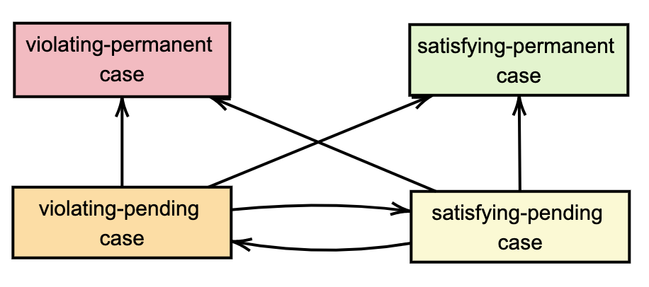
Figure 4: A transition diagram of the different states that a case could be in with respect to some constraint. The diagram shows the possible ways the state of a case can change as time progresses. Not shown in the diagram is that a case can also simply cease to be a case; furthermore, new cases appear.

Example 4 (Monitoring “Followed-By” Constraint)

Consider a process that comprises three activities with the labels $A,B$, and $C$ whose process model is shown in Figure 5. Let the constraint that is imposed on this process be “Every instance of activity $A$ must be directly followed by an instance of activity $B$ within 20 hours”. In Figure 6, we show five traces of that process which correspond to five cases as the constraint is an intra-instance one. The states of those five traces are distributed among the four different states.

Figure 5: A process model of an example process.

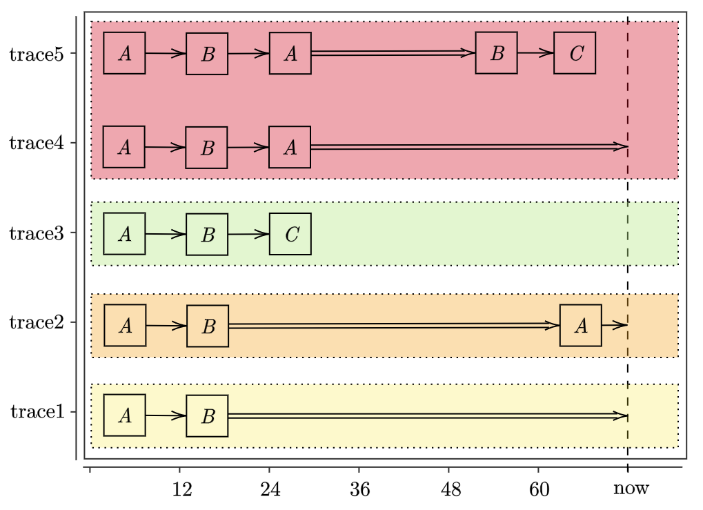
Figure 6: The plot contains five different traces of the process whose model is shown in Figure 5. The x-axis represents 12-hour intervals. In a trace, double arrows ($\Rightarrow$) (respectively, single arrows ($\rightarrow$)) denote time intervals that are longer (respectively, equal or shorter) than 20 hours. Each of the five traces is coloured based on its state at the “now” point with regard to the constraint “Every instance of activity $A$ must be directly followed by an instance of activity $B$ within 20 hours”. For an example, the fifth trace is in a violating-permanent state as the time span between the second execution of activities $A$ and $B$ is greater than the 20-hour interval.

Definition 2 (Constraint, Compliance monitoring Variant)

A constraint $C$ is represented by four queries $(Q_{\mathrm{case}},Q_{\mathrm{viol-perm}},$ $Q_{\mathrm{viol-pending}},Q_{\mathrm{sat-pending}})$, where $Q_{\mathrm{case}}$ returns all the cases subjected to the constraint $C$, $Q_{\mathrm{viol-perm}}$ returns the permanently violating cases, $Q_{\mathrm{viol-pending}}$ returns the violating cases that later could be changed to non-violating cases, while $Q_{\mathrm{sat-pending}}$ returns the satisfying cases that later could be changed to violating cases. (The cases not returned by none of these three queries, are then the ones defined by $Q_{\mathrm{sat-perm}}$.) On any database instance, $Q_{\mathrm{viol-perm}}$, $Q_{\mathrm{viol-pending}}$, and $Q_{\mathrm{sat-pending}}$ always return three mutually exclusive subsets of $Q_{\mathrm{case}}$.

Remark 3

Typically the query $Q_{\mathrm{viol}}$ in the post-mortem checking variant corresponds to the union of the pair $Q_{\mathrm{viol-perm}}$ and $Q_{\mathrm{viol-pending}}$ in the compliance monitoring variant. Similarly, the query $Q_{\mathrm{sat}}$ corresponds to the pair $Q_{\mathrm{sat-perm}}$ and $Q_{\mathrm{sat-pending}}$.

Example 5 (Monitoring Same Shipping Car Constraint)

Consider the same constraint as in Example 2. The queries representing this constraint can be defined as follows (where, $Q_{\mathrm{case}}$ and $Q_{\mathrm{viol-perm}}$ are defined as $Q_{\mathrm{case}}$ and $Q_{\mathrm{viol}}$ of Example 2; respectively.):

⬇

– Q_sat-pending

SELECT e.CarId, DATE(l.Timestamp)

FROM Log l, EventData e

WHERE l.EventId=e.EventId AND

l.ActivityLabel=’deliver package’ AND

l.Lifecycle=’complete’ AND e.Lifecycle=’complete’ AND

DATE(l.Timestamp)=CURRENT_DATE

GROUP BY e.CarId, DATE(l.Timestamp)

HAVING COUNT(e.PackageId) <= 7;

Note that $Q_{\mathrm{viol-pending}}$ will always be empty for this constraint.

4 Experiments

DBToaster is a state-of-the-art incremental query processor [23, 24, 33]. As a proof-of-concept of our approach, we tested DBToaster on some of the constraints from the work of Winter et al. on automatic discovery of ISC [35]. Specifically, we worked with the constraints ISC1, ISC2a, ISC2b, ISC3, and ISC4 from the paper. We have also used the execution logs provided by these authors as sample input data [10]. To manage our experiments, we performed some preprocessing steps that are mentioned in the Appendix 0.A. To assess the feasibility and usability of our approach, we have designed some experiments that ran over the mentioned five constraints. The results of these experiments are discussed in Sections 4.2, 4.3, and 4.4. At the beginning, we give a brief demonstration on the processes and the constraints used in the experiments in Section 4.1.

4.1 Experiment Data

The constraints used in the experiments are expressed over the three processes whose models are shown in Figure 7. In the Figure, we have “Flyer Order”, “Poster Order”, and “Bill” processes that are labelled as $P1$, $P3$, and $P2$, respectively.

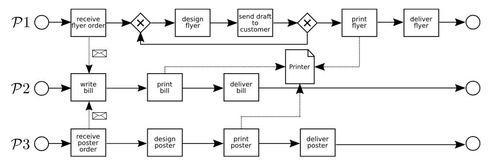
Figure 7: A figure showing the three process models whose executions are used in the experiments [35].

The “Flyer Order” process and “Poster Order” process are quite similar. Both processes begin by the activity of receiving the order. This is followed by designing the order activity, that is later followed by printing the order. In the end, the printed order is delivered. The only difference between the two processes is the extra activity of sending the design to the customer for confirmation before the printing proceeds. This is only part of the “Flyer Order” process. The customer either accepts the design, then the process proceeds as already mentioned. Otherwise, if the customer rejects the design then the order is redesigned and the same happens until the customer is satisfied with the flyer design. That explains the loop appearing in $P1$. Any order whether it is for a flyer or a poster, has a corresponding initiated “Bill” process. This process is quite simple, it begins by the activity of writing the bill, then the bill is printed and later delivered. Moreover, as you can see from the Figure, the printers are considered a shared resource between all the processes.

The constraints used in the experiments are the following:

ISC1 There is exactly one delivery activity per day in which all the finished orders/bills of that day so far are delivered to the post office simultaneously.

ISC2a All print jobs must be completed within 10 minutes in at least 95% of all cases per month.

ISC2b Printer 1 may only print 10 times per day.

ISC3 If a flyer or poster order is received $P2$ (i.e., bill process) is started afterwards. Moreover, the corresponding bill process must be started before the order is delivered to the post office.

ISC4 Printing jobs that require different paper formats (i.e., A4 and Poster formats) cannot be printed concurrently on one printer where concurrently means that one job starts, and before it finishes, the other starts.

We slightly modified the original constraints [35] to better match with the log data [10].

4.2 Running Time

The running time of three of the five monitored constraints is reported in Figure 8, which shows averages over 10 runs. The time is reported for every 300 insertions with total insertions 30636 (the number of events in the dataset). This experiment was performed on a personal laptop running macOS 12.2.1 with RAM of 16 GB and processor speed of 2.6Hz.

Figure 8: A plot of the running time (in milliseconds) taken to monitor the constraints ISC1, ISC3 and ISC4. The running time of the constraints ISC2a and ISC2b are omitted since they are quite similar to ISC4.

The slope of each curve is indicative of the average time needed, per event, to maintain the queries defining the constraint. We can see that this line is significantly higher for the first constraint; indeed, this constraint requires rather complex SQL queries (shown in Appendix 0.B). For tested constraints ISC1 and ISC3, the slopes of these lines are less than half a millisecond, respectively less than 1/6th of a millisecond. For tested constraints ISC2a, ISCb and ISC4, the slopes are less than 1% of a millisecond.

4.3 Sizes of Queries

The size (i.e., the number of cases) of each of the queries defining four of the five monitored constraints is reported and plotted relative to time (i.e., the number of insertions). This can show us how the cases are changing their status (pending or permanent, violating or satisfying). A plot for each of the four constraints is provided by Figure 9. The query size is reported every 500 insertions except for ISC2a which is done every 100 insertions instead, as it displays a more fine-grained behavior.

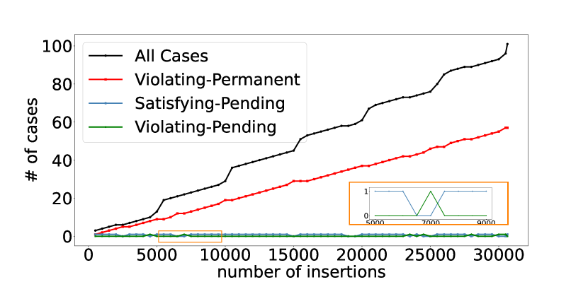
(a) Plot of ISC1

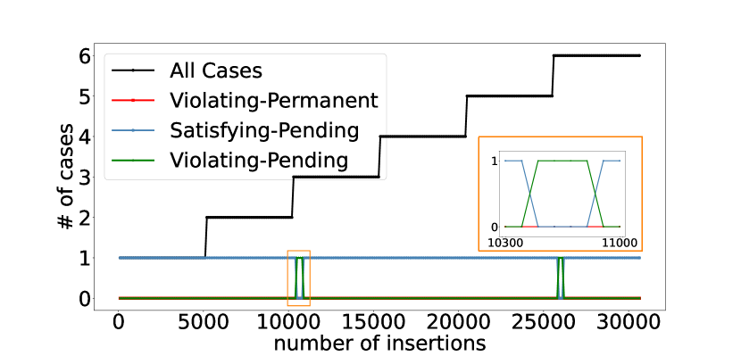
(b) Plot of ISC2a

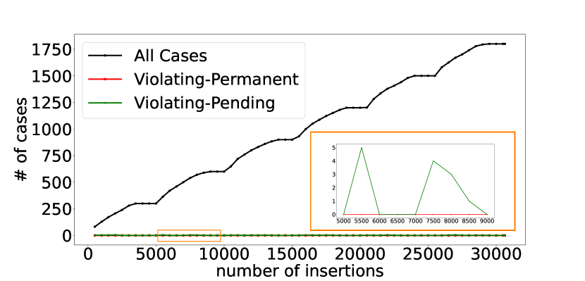
(c) Plot of ISC3

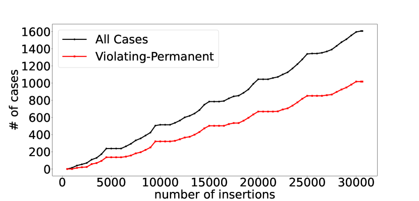
(d) Plot of ISC4

Figure 9: Plots of the size of each of the queries of the tested constraints. ISC2b is not shown as it has the same cases as ISC1 and has similar behavior to ISC3, which are shown. Since our measurements consist of 600 data points (even 3000 for ISC2a), the plots are at rather high scale. To show more detail, we provide insets that zoom in on selected regions (orange rectangles).

4.4 Tracing Cases

For ISC2a and ISC1, we show in Figures 10 and 11 the evolution in status of all the individual cases over time. This illustrates that our approach is compatible with monitoring on a very detailed level.

Figure 10: A plot showing the different cases of ISC2a and how each of the cases is changing its status through time. From the previous plots, we see that in total we have six cases for this constraint. The cases according to this constraint are months.

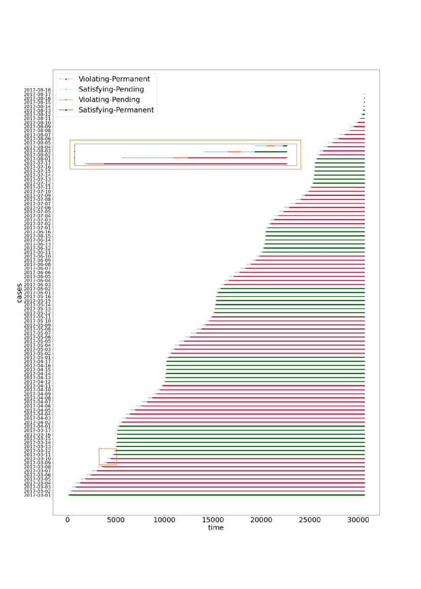
Figure 11: A plot showing the 101 different cases (days) of ISC1 and how each of the cases is changing its status through time. Here the measurement consists of 30600 data points per case, so the plot is at a very high scale. The inset shows more detail by zooming on the selected region (orange rectangle).

5 Sequence Data Extensions of Query Languages

We have mentioned before that any data model with a sufficiently expressive query language can be used to express the constraints. Although, we chose to work with the relational data model with SQL for the reasons we mentioned, it is interesting to briefly discuss query languages for the relational data model extended with sequences [4, 32]. Indeed, a trace is a sequence of events. Hence, representing the relative order of the events is quite natural in a sequence data model. This level of abstraction, of viewing traces as sequences of abstract events, is often assumed when working with temporal and dynamic logics [16, 30, 17].

Sequence Datalog [3, 6, 27] is an extension of the query language Datalog, to work with sequences as first class citizens. We will briefly showcase this language by considering a typical example of a constraint that is handled using the temporal logic.

Example 6 (Strict Sequencing [16])

Let $\mathtt{a}$ and $\mathtt{b}$ be two activities. Consider that we want to verify that the two activities are restricted by a strict sequencing relation, which is one of the standard ordering relations [2]. There is a strict sequencing relation between $\mathtt{a}$ and $\mathtt{b}$ if the log satisfies the following:

• there exists a trace where $\mathtt{a}$ is immediately followed by $\mathtt{b}$; and

• there are not any traces where $\mathtt{b}$ is immediately followed by $\mathtt{a}$.

There are two possible violations of this constraint. The first is not having a trace with $\mathtt{b}$ directly following $\mathtt{a}$. The other is having a trace with $\mathtt{a}$ directly following $\mathtt{b}$.

For the purpose of expressing this constraint, assume we have the following schema for the $\mathtt{Log}$ relation: $\mathtt{(TraceId,Events)}$, where $\mathtt{Events}$ are just a sequence of labels of activities. Then, this constraint can be expressed by the following Sequence Datalog program.

⬇

a_before_b():- Log(@traceId, $pre.a.b.$post).

violation():- +a_before_b().

violation():- Log(@traceId, $pre.b.a.$post).

This program illustrates a number of Sequence Datalog features:

• the dot is the concatenation operator.

• @traceId is an atomic variable (indicated by the @ symbol) representing atomic values (in this case, trace identifiers).

• $pre and $post are sequence variables (indicated by the $ symbol) representing (possibly empty) sequences of atomic values.

The utility of using Sequence Datalog can be appreciated if we compare the above program with the same query expressed in SQL.

⬇

(

SELECT 0

FROM Log l1, Log l2

WHERE l1.TraceId=l2.TraceId AND l1.Timestamp < l2.Timestamp AND

l1.ActivityLabel=’b’ AND l2.ActivityLabel=’a’ AND

NOT EXISTS

(

SELECT *

FROM Log l3

WHERE l1.TraceId=l3.TraceId AND

l1.Timestamp < l3.Timestamp AND

l3.Timestamp < l2.Timestamp

)

)

UNION

(

SELECT 0

WHERE NOT EXISTS

(

SELECT 0

FROM Log l1, Log l2

WHERE l1.TraceId=l2.TraceId AND l1.Timestamp < l2.Timestamp AND

l1.ActivityLabel=’a’ AND l2.ActivityLabel=’b’ AND

NOT EXISTS

(

SELECT *

FROM Log l3

WHERE l1.TraceId=l3.TraceId AND

l1.Timestamp < l3.Timestamp AND

l3.Timestamp < l2.Timestamp

)

)

);

6 Discussion

In this paper, we have looked into the problems of post-mortem checking and compliance monitoring of constraints over business processes. Specifically, we focused on ISC as recently introduced in the process mining field, and caught attention since it refers to complex constraints that span multiple process instances. Although there have been extensive works on inventorying and categorizing ISCs [31, 35], a crisp definition of what is or is not an ISC, however, seems to be elusive. Indeed, the notion of constraint is so broad that we propose to define any constraint as two or four queries posed against the database instance that represents a (partial) execution log. This approach gives us huge flexibility, moreover, we gain a lot from advances in database technology as demonstrated in the Experiments Section.

In using the DBToaster system for our experiments, we faced a few technical issues. The main challenge was that the Scala version of DBToaster gets stuck when retrieving snapshots over the course of the insertions. To overcome this issue, to perform our measurements of counting cases over time, and how they evolve their constraint satisfaction status, we only retrieved a snapshot after an initial sequence of insertions. We then restart the measurement for one batch of insertions longer. Another limitation is that SQL is not yet fully supported, although complex queries can be expressed. This required us to sometimes rewrite queries in equivalent form. Finally, some built-in functions (e.g., on strings or dates) are missing from the Scala version. Thus, those experiments should be seen more of a proof-of-concept of the feasibility of our approach.

In this discussion, we briefly touch upon the main difference between our approach and the main approach that is used to monitor ISC. This approach is based on the Event Calculus (EC) [25, 28, 22]. Most monitoring systems that are based on EC are implemented using Prolog. Using EC to express a constraint seems to be very procedural albeit being defined in logical programming language. For example, to monitor a constraint such as ISC2b, in EC one would define a rule that increments a counter every time a printing event occurs. At the end, that counter value should be at most 10 as per the constraint. Since this is done in Prolog, this will be asking the SAT solver if there exists an extension of the given sequence of events satisfying the specification of this counting process. A similar approach was followed in the paper by Montali et al. [28] to monitor business (intra-instance) constraint with the EC. Events come in time, and Prolog rules that fire every new time instant, are used to check various constraints dynamically. However, these incremental rules are manually implemented. On the contrary, using an incremental query processor shifts the focus on what the queries (or constraints) themselves are rather than what the rules are that are responsible for this incremental maintenance. Hence, our approach is more declarative.

At the end of this discussion, we mention a few points for further research. Since there are some algorithms that are used to discover ISC from execution logs [35], and these algorithms search for explicit patterns, one could define a common language to report the results of those algorithms and use those results to automatically write the SQL queries monitoring each of the reported constraints. Thus, the whole process could be automated. Also, one could try to rewrite the same queries differently and evaluate how the different formulations affect the running times to incrementally maintain them.

Acknowledgments

We thank Stefanie Rinderle-Ma and Jürgen Mangler for initial discussions.

Appendix 0.A Experiments Preprocessing

As mentioned in the main paper, we performed the following preprocessing steps to manage our experiments:

1. The execution logs are given in XES format; we converted them to CSV using the process mining python library PM4Py [15].

2. The events from the different processes are merged and sorted based on the timestamp attribute. In this way, we simulate a stream of events suitable for monitoring.

3. For each of the selected constraints, we formulated appropriate SQL queries defining the cases, the violations, the pending violations, and the pending satisfying cases, following our methodology described in Definition 2.

4. DBToaster takes these queries and produces an executable program (JAR file) that allows to communicate with the queries while being incrementally maintained.

5. Lastly, we have implemented a Scala program for each of the constraints that reads the CSV file and communicates with the incremental processor from Step 4 by sending the events as insertions and asking for the intermediate results of the queries.

Appendix 0.B SQL Queries of Constraints

We begin this section by Table 1 that summarizes the SQL features used in the monitored constraints. In our queries, we use a view Events which is defined by the natural join of Log and EventData. Afterwards, we show these SQL queries.

Table 1: A table showing the SQL features used in the queries expressing each of the monitored five constraints.

ISC	Aggregation	OR	Existence Check	Negation	Double Negation
ISC1	no	no	yes	yes	yes
ISC2a	yes	no	yes	yes	no
ISC2b	yes	no	no	yes	no
ISC3	no	yes	yes	yes	no
ISC4	no	no	no	yes	no

0.B.1 Queries of ISC1

⬇

– Q_case

SELECT DISTINCT(DATE(Timestamp)) FROM Events;

– Q_viol

SELECT DATE(e.Timestamp)

FROM Events e, Events e4

WHERE e.Lifecycle = ’start’ AND e.ActivityLabel LIKE ’deliver%’

AND DATE(e.Timestamp) = DATE(e4.Timestamp)

AND e.Timestamp < e4.Timestamp

AND ( EXISTS

( SELECT *

FROM Events e2

WHERE DATE(e.Timestamp) = DATE(e2.Timestamp)

AND e2.Lifecycle = ’complete’

AND e2.ActivityLabel LIKE ’print%’

AND e2.Timestamp < e.Timestamp

AND ( NOT EXISTS

( SELECT *

FROM Events e3

WHERE e3.ProcessId = e2.ProcessId

AND e3.TraceId = e2.TraceId

AND e3.ActivityLabel LIKE ’deliver%’

AND e3.Lifecycle = ’start’

AND e3.Timestamp = e.Timestamp

) ) ) );

– Q_sat-pending

SELECT DATE(c.Timestamp)

FROM CURR_DAY c

WHERE DATE(c.Timestamp) NOT IN

( SELECT DATE(e.Timestamp)

FROM Events e

WHERE e.Lifecycle = ’start’ AND e.ActivityLabel LIKE ’deliver%’

AND ( ( EXISTS

( SELECT *

FROM Events e2

WHERE DATE(e.Timestamp) = DATE(e2.Timestamp)

AND e2.Lifecycle = ’complete’

AND e2.ActivityLabel LIKE ’print%’

AND e2.Timestamp < e.Timestamp

AND ( NOT EXISTS

( SELECT *

FROM Events e3

WHERE e3.ProcessId = e2.ProcessId

AND e3.TraceId = e2.TraceId

AND e3.ActivityLabel LIKE ’deliver%’

AND e3.Lifecycle = ’start’

AND e3.Timestamp = e.Timestamp

) ) ) ) ) );

– Q_viol-pending

SELECT DATE(c.Timestamp)

FROM CURR_DAY c, Events e

WHERE e.Lifecycle = ’start’ AND e.ActivityLabel LIKE ’deliver%’

AND DATE(e.Timestamp) = DATE(c.Timestamp)

AND ( EXISTS

( SELECT *

FROM Events e2

WHERE DATE(e.Timestamp) = DATE(e2.Timestamp)

AND e2.Lifecycle = ’complete’

AND e2.ActivityLabel LIKE ’print%’

AND e2.Timestamp < e.Timestamp

AND ( NOT EXISTS

( SELECT *

FROM Events e3

WHERE e3.ProcessId = e2.ProcessId

AND e3.TraceId = e2.TraceId

AND e3.ActivityLabel LIKE ’deliver%’

AND e3.Lifecycle = ’start’

AND e3.Timestamp = e.Timestamp

) ) ) )

AND ( NOT EXISTS

( SELECT *

FROM Events e4

WHERE DATE(e.Timestamp) = DATE(e4.Timestamp)

AND e.Timestamp < e4.Timestamp

) );

0.B.2 Queries of ISC2a

In these queries, we use the terminology of $\tt e.Year$, $\tt e.Month$, $\tt e.Hour$, and $\tt e.Minute$ for some $\tt Event\,e$. You can consider these as shortcuts for the following clauses, receptively:

• $\tt EXTRACT(Year\,FROM\,e.Timestamp)$,

• $\tt EXTRACT(Month\,FROM\,e.Timestamp)$,

• $\tt EXTRACT(Hour\,FROM\,e.Timestamp)$, and

• $\tt EXTRACT(Minute\,FROM\,e.Timestamp)$.

⬇

– Q_case

SELECT m.Year, m.Month

FROM (

SELECT e1.Year, e1.Month, COUNT(*) AS NumberOfMonthCases,

SUM( CASE WHEN ((((e2.Hour - e1.Hour) * 60) +

(e2.Minute - e1.Minute)) > 10)

THEN 0 ELSE 1 END) AS NumberOfMonthFastCases

FROM Events e1, Events e2

WHERE e1.ProcessId = e2.ProcessId AND e1.TraceId = e2.TraceId AND

e1.Lifecycle = ’start’ AND e2.Lifecycle = ’complete’ AND

e1.ActivityLabel LIKE ’print%’ AND e2.ActivityLabel LIKE ’print%’

GROUP BY e1.Year, e1.Month

) as m;

– Q_viol

SELECT m.Year, m.Month

FROM (

SELECT e1.Year, e1.Month, COUNT(*) AS NumberOfMonthCases,

SUM( CASE WHEN ((((e2.Hour - e1.Hour) * 60) +

(e2.Minute - e1.Minute)) > 10)

THEN 0 ELSE 1 END) AS NumberOfMonthFastCases

FROM Events e1, Events e2

WHERE e1.ProcessId = e2.ProcessId AND e1.TraceId = e2.TraceId AND

e1.Lifecycle = ’start’ AND e2.Lifecycle = ’complete’ AND

e1.ActivityLabel LIKE ’print%’ AND e2.ActivityLabel LIKE ’print%’

GROUP BY e1.Year, e1.Month

) as m

WHERE (m.NumberOfMonthFastCases*100/m.NumberOfMonthCases) <= 95

AND NOT EXISTS

( SELECT * FROM CURR_MONTH c

WHERE c.Year = m.YEAR AND c.Month = m.Month );

– Q_sat-pending

SELECT m.Year, m.Month

FROM (

SELECT e1.Year, e1.Month, COUNT(*) AS NumberOfMonthCases,

SUM( CASE WHEN ((((e2.Hour - e1.Hour) * 60) +

(e2.Minute - e1.Minute)) > 10)

THEN 0 ELSE 1 END) AS NumberOfMonthFastCases

FROM Events e1, Events e2

WHERE e1.ProcessId = e2.ProcessId AND e1.TraceId = e2.TraceId AND

e1.Lifecycle = ’start’ AND e2.Lifecycle = ’complete’ AND

e1.ActivityLabel LIKE ’print%’ AND e2.ActivityLabel LIKE ’print%’

GROUP BY e1.Year, e1.Month

) as m

WHERE (m.NumberOfMonthFastCases*100/m.NumberOfMonthCases) > 95

AND EXISTS

( SELECT * FROM CURR_MONTH c

WHERE c.Year = m.Year AND c.Month = m.Month );

– Q_viol-pending

SELECT m.Year, m.Month

FROM (

SELECT e1.Year, e1.Month, COUNT(*) AS NumberOfMonthCases,

SUM( CASE WHEN ((((e2.Hour - e1.Hour) * 60) +

(e2.Minute - e1.Minute)) > 10)

THEN 0 ELSE 1 END) AS NumberOfMonthFastCases

FROM Events e1, Events e2

WHERE e1.ProcessId = e2.ProcessId AND e1.TraceId = e2.TraceId AND

e1.Lifecycle = ’start’ AND e2.Lifecycle = ’complete’ AND

e1.ActivityLabel LIKE ’print%’ AND e2.ActivityLabel LIKE ’print%’

GROUP BY e1.Year, e1.Month

) as m

WHERE (m.NumberOfMonthFastCases*100/m.NumberOfMonthCases) <= 95

AND EXISTS

( SELECT * FROM CURR_MONTH c

WHERE c.Year = m.Year AND c.Month = m.Month );

0.B.3 Queries of ISC2b

⬇

– Q_case

SELECT DISTINCT(DATE(Timestamp)) FROM Events;

– Q_viol

SELECT DATE(t.Timestamp)

FROM (

SELECT DATE(e.Timestamp), COUNT(e.TraceId) AS Uses

FROM Events e

WHERE e.Lifecycle = ’complete’ AND e.ActivityLabel LIKE ’print%’

AND e.Resource = ’printer1’

GROUP BY DATE(e.Timestamp)

) AS t

WHERE t.Uses > 10;

– Q_sat-pending

SELECT DATE(c.Timestamp)

FROM CURR_DAY c

WHERE c.Date NOT IN (

SELECT DATE(t.Timestamp)

FROM (

SELECT DATE(e.Timestamp), COUNT(e.TraceId) AS Uses

FROM Events e

WHERE e.Lifecycle = ’complete’ AND e.ActivityLabel LIKE ’print%’

AND e.Resource = ’printer1’

GROUP BY DATE(e.Timestamp)

) AS t

WHERE t.Uses > 10

);

0.B.4 Queries of ISC3

⬇

– Q_case

SELECT ProcessId, TraceId FROM Events

WHERE ActivityLabel LIKE ’receive %’;

– Q_viol

SELECT e1.ProcessId, e1.TraceId

FROM Events e1

WHERE e1.ActivityLabel LIKE ’receive %’ AND e1.Lifecycle = ’start’ AND

(

(

( EXISTS ( SELECT * FROM Events e2

WHERE e1.ProcessId = e2.ProcessId

AND e1.TraceId = e2.TraceId

AND e2.ActivityLabel LIKE ’deliver %’

AND e2.Lifecycle = ’complete’ ) )

AND

( NOT EXISTS ( SELECT * FROM Events e3

WHERE e3.ActivityLabel LIKE ’write bill’

AND e3.CustomerId = e1.CustomerId ) )

) – P2 is not yet started but the order is delivered

OR

( EXISTS ( SELECT * FROM Events e4

WHERE e4.ActivityLabel LIKE ’write bill’

AND e4.CustomerId = e1.CustomerId

AND e4.Timestamp < e1.Timestamp )

) – P2 is started before the order being received

);

– Q_viol-pending

SELECT e1.ProcessId, e1.TraceId

FROM Events e1

WHERE e1.ActivityLabel LIKE ’receive %’ AND e1.Lifecycle = ’start’

AND

( NOT EXISTS (

SELECT * FROM Events e2

WHERE e1.ProcessId = e2.ProcessId AND e1.TraceId = e2.TraceId

AND e2.ActivityLabel LIKE ’deliver %’

AND e2.Lifecycle = ’complete’ ) )

AND

( NOT EXISTS (

SELECT * FROM Events e3

WHERE e3.ActivityLabel LIKE ’write bill’

AND e3.CustomerId = e1.CustomerId )

);

0.B.5 Queries of ISC4

⬇

– Q_case

SELECT e1.ProcessId, e1.TraceId, e3.ProcessId, e3.TraceId

FROM Events e1, Events e3

WHERE e1.ActivityLabel LIKE ’print%’ AND e3.ActivityLabel LIKE ’print%’

AND e1.Lifecycle = ’start’AND e3.Lifecycle = ’start’

AND DATE(e1.Timestamp) = DATE(e3.Timestamp)

AND e1.Timestamp < e3.Timestamp

AND (

NOT EXISTS (

SELECT * FROM Events e2

WHERE e1.ProcessId = e2.ProcessId AND e1.TraceId = e2.TraceId

AND e2.ActivityLabel LIKE ’print%’

AND e2.Lifecycle = ’complete’

AND e1.Timestamp < e2.Timestamp

AND e2.Timestamp < e3.Timestamp

) );

– Q_viol

SELECT e1.ProcessId, e1.TraceId, e3.ProcessId, e3.TraceId

FROM Events e1, Events e3

WHERE e1.ActivityLabel LIKE ’print%’ AND e3.ActivityLabel LIKE ’print%’

AND e1.Lifecycle = ’start’ AND e3.Lifecycle = ’start’

AND DATE(e1.Timestamp) = DATE(e3.Timestamp)

AND e1.Timestamp < e3.Timestamp

AND (

NOT EXISTS (

SELECT * FROM Events e2

WHERE e1.ProcessId = e2.ProcessId AND e1.TraceId = e2.TraceId

AND e2.ActivityLabel LIKE ’print%’

AND e2.Lifecycle = ’complete’

AND e1.Timestamp < e2.Timestamp

AND e2.Timestamp < e3.Timestamp

) )

AND e1.Format <> e3.Format AND e1.Resource = e3.Resource;

References

- [1] van der Aalst, W.M.P.: Process Mining: Overview and Opportunities. ACM Trans. Manag. Inf. Syst. 3(2), 7:1–7:17 (2012). https://doi.org/10.1145/2229156.2229157
- [2] van der Aalst, W.M.P., Weijters, T., Maruster, L.: Workflow mining: Discovering process models from event logs. IEEE Trans. Knowl. Data Eng. 16(9), 1128–1142 (2004). https://doi.org/10.1109/TKDE.2004.47
- [3] Aamer, H., Hidders, J., Paredaens, J., Van den Bussche, J.: Expressiveness within Sequence Datalog. In: Libkin, L., Pichler, R., Guagliardo, P. (eds.) PODS’21: Proceedings of the 40th ACM SIGMOD-SIGACT-SIGAI Symposium on Principles of Database Systems, Virtual Event, China, June 20-25, 2021. pp. 70–81. ACM (2021). https://doi.org/10.1145/3452021.3458327
- [4] Angles, R., Arenas, M., Barceló, P., Boncz, P.A., Fletcher, G.H.L., Gutiérrez, C., Lindaaker, T., Paradies, M., Plantikow, S., Sequeda, J.F., van Rest, O., Voigt, H.: G-CORE: A Core for Future Graph Query Languages. In: Das, G., Jermaine, C.M., Bernstein, P.A. (eds.) Proceedings of the 2018 International Conference on Management of Data, SIGMOD Conference 2018, Houston, TX, USA, June 10-15, 2018. pp. 1421–1432. ACM (2018). https://doi.org/10.1145/3183713.3190654
- [5] Bauer, A., Leucker, M., Schallhart, C.: Runtime verification for LTL and TLTL. ACM Trans. Softw. Eng. Methodol. 20(4), 14:1–14:64 (2011)
- [6] Bonner, A., Mecca, G.: Sequences, Datalog, and Transducers. J. Comput. Syst. Sci. 57, 234–259 (1998)
- [7] Calvanese, D., De Giacomo, G., Montali, M., Patrizi, F.: Verification and monitoring for first-order LTL with persistence-preserving quantification over finite and infinite traces. In: Proceedings of the 31st International Conference on Artificial Intelligence (IJCAI-ECAI 2022). AAAI Press (2022), to appear
- [8] Cardoso, E., Montali, M., Calvanese, D.: Representing and querying norm states using temporal ontology-based data access. In: Proceedings of the 23rd IEEE International Enterprise Distributed Object Computing Conference (EDOC 2019). pp. 122–131. IEEE (2019)
- [9] Chirkova, R., Yang, J.: Materialized Views. Foundations and Trends® in Databases 4(4), 295–405 (2012). https://doi.org/10.1561/1900000020
- [10] CRISP project at Universität Wien: Execution Logs Webpage. http://gruppe.wst.univie.ac.at/projects/crisp/index.php?t=discovery, accessed: 2022-04-29
- [11] De Giacomo, G., De Masellis, R., Grasso, M., Maggi, F.M., Montali, M.: Monitoring business metaconstraints based on LTL and LDL for finite traces. In: Sadiq, S.W., Soffer, P., Völzer, H. (eds.) Proceedings of the 12th International Conference on Business Process Management (BPM 2014). Lecture Notes in Computer Science, vol. 8659, pp. 1–17. Springer (2014)
- [12] De Giacomo, G., De Masellis, R., Maggi, F.M., Montali, M.: Monitoring constraints and metaconstraints with temporal logics on finite traces. ACM Trans. Softw. Eng. Methodol. (2022), to appear
- [13] Demri, S., Lazic, R.: LTL with the freeze quantifier and register automata. ACM Trans. on Computational Logic 10(3) (2009)
- [14] Fdhila, W., Gall, M., Rinderle-Ma, S., Mangler, J., Indiono, C.: Classification and Formalization of Instance-Spanning Constraints in Process-Driven Applications. In: Rosa, M.L., Loos, P., Pastor, O. (eds.) Business Process Management - 14th International Conference, BPM 2016, Rio de Janeiro, Brazil, September 18-22, 2016. Proceedings. Lecture Notes in Computer Science, vol. 9850, pp. 348–364. Springer (2016). https://doi.org/10.1007/978-3-319-45348-4_20
- [15] Fraunhofer Institute for Applied Information Technology (FIT): PM4Py Website. https://pm4py.fit.fraunhofer.de/, accessed: 2022-04-29
- [16] Giacomo, G.D., Felli, P., Montali, M., Perelli, G.: HyperLDLf: a Logic for Checking Properties of Finite Traces Process Logs. In: Zhou, Z. (ed.) Proceedings of the Thirtieth International Joint Conference on Artificial Intelligence, IJCAI 2021, Virtual Event / Montreal, Canada, 19-27 August 2021. pp. 1859–1865. ijcai.org (2021). https://doi.org/10.24963/ijcai.2021/256
- [17] Giacomo, G.D., Masellis, R.D., Grasso, M., Maggi, F.M., Montali, M.: Monitoring Business Metaconstraints Based on LTL and LDL for Finite Traces. In: Sadiq, S.W., Soffer, P., Völzer, H. (eds.) Business Process Management - 12th International Conference, BPM 2014, Haifa, Israel, September 7-11, 2014. Proceedings. Lecture Notes in Computer Science, vol. 8659, pp. 1–17. Springer (2014). https://doi.org/10.1007/978-3-319-10172-9_1
- [18] Gupta, A., Mumick, I.S. (eds.): Materialized Views: Techniques, Implementations, and Applications. MIT Press, Cambridge, MA, USA (1999)
- [19] Gupta, A., Mumick, I.S.: Maintenance of Materialized Views: Problems, Techniques, and Applications. IEEE Data Eng. Bull. 18(2), 3–18 (1995), http://sites.computer.org/debull/95JUN-CD.pdf
- [20] Gupta, A., Mumick, I.S., Subrahmanian, V.S.: Maintaining Views Incrementally. In: Buneman, P., Jajodia, S. (eds.) Proceedings of the 1993 ACM SIGMOD International Conference on Management of Data, Washington, DC, USA, May 26-28, 1993. pp. 157–166. ACM Press (1993). https://doi.org/10.1145/170035.170066
- [21] IEEE XES Group: IEEE 1849-2016 XES Standard. https://www.xes-standard.org/, accessed: 2022-05-11
- [22] Indiono, C., Mangler, J., Fdhila, W., Rinderle-Ma, S.: Rule-Based Runtime Monitoring of Instance-Spanning Constraints in Process-Aware Information Systems. In: Debruyne, C., Panetto, H., Meersman, R., Dillon, T.S., eva Kühn, O’Sullivan, D., Ardagna, C.A. (eds.) On the Move to Meaningful Internet Systems: OTM 2016 Conferences - Confederated International Conferences: CoopIS, C&TC, and ODBASE 2016, Rhodes, Greece, October 24-28, 2016, Proceedings. Lecture Notes in Computer Science, vol. 10033, pp. 381–399 (2016). https://doi.org/10.1007/978-3-319-48472-3_22
- [23] Kennedy, O., Ahmad, Y., Koch, C.: DBToaster: Agile Views for a Dynamic Data Management System. In: Fifth Biennial Conference on Innovative Data Systems Research, CIDR 2011, Asilomar, CA, USA, January 9-12, 2011, Online Proceedings. pp. 284–295. www.cidrdb.org (2011), http://cidrdb.org/cidr2011/Papers/CIDR11_Paper38.pdf
- [24] Koch, C., Ahmad, Y., Kennedy, O., Nikolic, M., Nötzli, A., Lupei, D., Shaikhha, A.: DBToaster: Higher-order Delta Processing for Dynamic, Frequently Fresh Views. VLDB J. 23(2), 253–278 (2014). https://doi.org/10.1007/s00778-013-0348-4
- [25] Ly, L.T., Maggi, F.M., Montali, M., Rinderle-Ma, S., van der Aalst, W.M.P.: Compliance Monitoring in Business Processes: Functionalities, Application, and Tool-Support. Inf. Syst. 54, 209–234 (2015). https://doi.org/10.1016/j.is.2015.02.007
- [26] Maggi, F.M., Montali, M., Westergaard, M., van der Aalst, W.M.P.: Monitoring business constraints with linear temporal logic: An approach based on colored automata. In: Rinderle-Ma, S., Toumani, F., Wolf, K. (eds.) Proceedings of the 9th International Conference on Business Process Management (BPM 2011). Lecture Notes in Computer Science, vol. 6896, pp. 132–147. Springer (2011)
- [27] Mecca, G., Bonner, A.: Query Languages for Sequence Databases: Termination and Complexity. IEEE Transactions on Knowledge and Data Engineering 13(3), 519–525 (2001)
- [28] Montali, M., Maggi, F.M., Chesani, F., Mello, P., van der Aalst, W.M.P.: Monitoring Business Constraints with the Event Calculus. ACM Trans. Intell. Syst. Technol. 5(1), 17:1–17:30 (2013). https://doi.org/10.1145/2542182.2542199
- [29] de Murillas, E.G.L., Reijers, H.A., van der Aalst, W.M.P.: Connecting databases with process mining: a meta model and toolset. Softw. Syst. Model. 18(2), 1209–1247 (2019). https://doi.org/10.1007/s10270-018-0664-7
- [30] Pesic, M., Schonenberg, H., van der Aalst, W.M.P.: DECLARE: Full Support for Loosely-Structured Processes. In: 11th IEEE International Enterprise Distributed Object Computing Conference (EDOC 2007), 15-19 October 2007, Annapolis, Maryland, USA. pp. 287–300. IEEE Computer Society (2007). https://doi.org/10.1109/EDOC.2007.14
- [31] Rinderle-Ma, S., Gall, M., Fdhila, W., Mangler, J., Indiono, C.: Collecting Examples for Instance-Spanning Constraints. arXiv:1603.01523 (2018)
- [32] Shen, W., Doan, A., Naughton, J.F., Ramakrishnan, R.: Declarative Information Extraction Using Datalog with Embedded Extraction Predicates. In: Koch, C., Gehrke, J., Garofalakis, M.N., Srivastava, D., Aberer, K., Deshpande, A., Florescu, D., Chan, C.Y., Ganti, V., Kanne, C., Klas, W., Neuhold, E.J. (eds.) Proceedings of the 33rd International Conference on Very Large Data Bases, University of Vienna, Austria, September 23-27, 2007. pp. 1033–1044. ACM (2007)
- [33] The DBToaster Consortium: DBToaster Webpage. https://dbtoaster.github.io/index.html, accessed: 2022-04-29
- [34] Warner, J., Atluri, V.: Inter-instance Authorization Constraints for Secure Workflow Management. In: Ferraiolo, D.F., Ray, I. (eds.) 11th ACM Symposium on Access Control Models and Technologies, SACMAT 2006, Lake Tahoe, California, USA, June 7-9, 2006, Proceedings. pp. 190–199. ACM (2006). https://doi.org/10.1145/1133058.1133085
- [35] Winter, K., Stertz, F., Rinderle-Ma, S.: Discovering Instance and Process Spanning Constraints from Process Execution Logs. Inf. Syst. 89, 101484 (2020). https://doi.org/10.1016/j.is.2019.101484