End-to-end Optimization of Machine Learning Prediction Queries

Abstract.

Prediction queries are widely used across industries to perform advanced analytics and draw insights from data. They include a data processing part (e.g., for joining, filtering, cleaning, featurizing the datasets) and a machine learning (ML) part invoking one or more trained models to perform predictions. These parts have so far been optimized in isolation, leaving significant opportunities for optimization unexplored.

We present Raven, a production-ready system for optimizing prediction queries. Raven follows the enterprise architectural trend of collocating data and ML runtimes. It relies on a unified intermediate representation that captures both data and ML operators in a single graph structure to unlock two families of optimizations. First, it employs logical optimizations that pass information between the data part (and the properties of the underlying data) and the ML part to optimize each other. Second, it introduces logical-to-physical transformations that allow operators to be executed on different runtimes (relational, ML, and DNN) and hardware (CPU, GPU). Novel data-driven optimizations determine the runtime to be used for each part of the query to achieve optimal performance. Our evaluation shows that Raven improves performance of prediction queries on Apache Spark and SQL Server by up to 13.1$\times$ and 330$\times$, respectively. For complex models where GPU acceleration is beneficial, Raven provides up to 8$\times$ speedup compared to state-of-the-art systems.

1. Introduction

Thanks to its recent advances, machine learning (ML) is being widely adopted in the enterprise and is on track to revolutionize every industry (Moore, 2016). Trained ML models are being deployed in a wide variety of scenarios, ranging from datacenters to edge devices and across the software stack (Sacolick, 2020), to capitalize on the immense possibilities ML offers by drawing patterns and insights from data.

High-value data in the enterprise is expressed, to a large extent, in structured or semi-structured forms (Compact.nl, 2021; Agrawal et al., 2020; Ilyas, 2021), typically stored in relational databases, data warehouses (Aguilar-Saborit et al., 2020; Amazon.com, 2021a; Dageville et al., 2016), or data lakes (Ramakrishnan et al., 2017; Armbrust et al., 2020). To train models on this data, data scientists often perform several pre-processing steps, e.g., to combine datasets (through unions, joins, aggregates), tokenize or unnest records, clean them, and encode them into features. Therefore, most widely used ML frameworks have added support for defining trained pipelines, i.e., Direct Acyclic Graphs (DAGs) of operators including ML models along with pre-processing steps (Meng et al., 2016; Scikit-learn, 2021a; Baylor et al., 2017; ONNX, 2021a; Ahmed et al., 2019).

ML inference in the enterprise. Data analysts and software engineers issue prediction queries, which are complex analytics queries that employ trained pipelines to perform predictions over new data arriving in the database/data lake. These queries often include additional data processing operators (e.g., filters or joins), implementing prediction-specific logic. As we discuss in § 2, ML inference drives the majority of the cost (up to 90% (Jassy, 2021)) associated with ML in the enterprise, whereas traditional ML models (i.e., non-neural networks, such as linear regression and tree-based models) are still the most widely used by a large margin (Kaggle, 2020; Psallidas et al., 2019). Moreover, based on the analysis of $130$ customer engagements at Microsoft, we found that batch inference is chosen over online inference in most enterprise scenarios. Not surprisingly, most cloud vendors have enabled issuing batch prediction queries through recent SQL extensions or traditional user-defined functions (UDFs) for inference (Microsoft, 2021e, g; Google, 2021a; Amazon.com, 2021b; Armbrust et al., 2015; Hellerstein et al., 2012). Therefore, in this work we focus on the optimization of batch prediction queries that invoke traditional ML models.

Optimization opportunities. We make two crucial observations that open untapped opportunities for the optimization of prediction queries. First, existing work has mainly focused on optimizing each part of the prediction queries in isolation (Chen et al., 2018; Lee et al., 2018a; Kraft et al., 2019). However, at their core, prediction queries are just a set of operations over data, which, treated holistically, offer great opportunities for optimization—we provide an analysis of hundreds of pipelines in § 2. With Raven’s initial version (Karanasos et al., 2020), we laid out our vision of optimizations spanning data and ML operators in prediction queries. However, in that initial prototype, a few limited optimizations were applied manually over simplistic single-operator models—our analysis in § 2 shows that such models are uncommon in practice. Recently, a few more works have started touching upon optimization across data and ML operators, but only in the context of training and generalized linear models (Boehm et al., 2016; Kunft et al., 2019; Wang et al., 2020; Kumar et al., 2015; Olteanu, 2020) or targeting their execution at the physical level (Palkar et al., 2018).

Second, most related research efforts consider a unified runtime to execute relational and ML queries (Boehm et al., 2016; Palkar et al., 2018; Kunft et al., 2019). In industry-grade data systems, however, we observe a different trend: while some of these ideas can be applied on parts of the query, production systems have steered away from running every ML workload natively. This is particularly true for complex data operations (e.g., tf.data allows only simple transformations (Murray et al., 2021)) or complex ML operations (linear algebra may be efficiently executed inside the database but covers small portion of prediction pipelines). Instead, modern data engines integrate with ML runtimes for breadth of ML support: Microsoft SQL Server/ONNX Runtime (Microsoft, 2021e), Google BigQuery/TensorFlow (Google, 2021a), Amazon Redshift/SageMaker (Amazon.com, 2021b).

We believe that the co-existence of specialized (software/hardware) accelerators into data runtimes is not the outcome of current technology limitations but an architecture that is here to stay. Thus, the natural question to ask is: having these ML runtimes next to the data engine, how and when should we exploit each runtime to accelerate prediction queries?

Raven Optimizer. Through this work, we substantially push the envelope in realizing and extending our Raven vision (Karanasos et al., 2020) for the optimization of prediction queries. Following the architecture of collocating data engines with ML accelerators, we present the optimizer that fuels Raven, which is the result of 10 people-years of work. Our optimizer (i) applies logical optimizations to holistically optimize the query; and (ii) judiciously picks which part of the plan to run on each engine. Concretely, we make the following contributions.

State of enterprise ML inference (§ 2). We provide several insights for the state of ML inference in the enterprise, based on findings from Microsoft, customer engagements, offerings from various cloud vendors, and an analysis of hundreds of publicly available pipelines. All these acted as a motivation for building Raven.

Logical optimizations (§ 4). Raven relies on a unified intermediate representation (IR) that captures both data and ML operators in a common structure (§ 3). It combines concepts from the relational algebra and similar efforts recently introduced by ML frameworks (namely, ONNX (ONNX, 2021a)). Having all operators of a prediction query in a single IR allows us to optimize the query holistically. In particular, we extend the cross-optimizations (first introduced in (Karanasos et al., 2020)) to support a wide range of models with multiple operators each, which are actually used in the enterprise (including several tree-based models, such as random forests and gradient boosting trees). We also introduce novel data-induced optimizations. Through these logical optimizations, Raven exploits features of data processing operators and data properties to avoid unnecessary computation in the ML part and vice-versa by flowing information between operators (Beeri and Ramakrishnan, 1987). For example, a data predicate on an input feature can be used to simplify the model at compile time, whereas input features that end up not participating in inference can be completely removed from the whole query.

Logical-to-physical: runtime selection (§ 5). The collocation of the data engine with ML accelerators allows Raven to assign different parts of the IR to the runtime that will lead to optimal performance. To this end, we employ logical-to-physical optimizations that can turn a classical ML model to an equivalent SQL statement (to be executed by the data engine) or to an equivalent neural network (to be executed by the ML accelerator, possibly on a GPU).

Most importantly, we show that these optimizations are not always beneficial: blindly applying them, as we did in the initial Raven prototype (Karanasos et al., 2020), can lead to slowdowns of up to 6$\times$. Hence, Raven introduces optimization strategies to pick the rules that would lead to best performance for each query on a given hardware setup. Instead of relying on hard-coded heuristics that do not work across workloads and hardware, Raven employs data-driven, instance-optimized strategies: a novel data-informed strategy and two ML-based ones.

An end-to-end system (§ 6). The Raven optimizer, which has been fully implemented as an extension to Apache Spark, is the first production-ready system to incorporate such optimizations. Users specify prediction queries in SparkSQL invoking models expressed in ONNX (or any format convertible to ONNX (ONNX, 2021b)). Raven’s optimizer with all the above optimizations and optimization strategies are implemented as a co-optimizer invoked by Spark’s Catalyst optimizer. We have also made it possible to execute Raven’s optimized plans in SQL Server.

We experimentally validate the benefits of Raven over a variety of datasets, prediction queries, and hardware (§ 7). Our results show significant performance gains on both Spark and SQL Server. In particular, Raven’s optimized plans achieve 1.4–13.1$\times$ speedup against Spark and 1.4–330x against SQL Server. We also report similar and even bigger gains against other state-of-the-art systems, such as MADlib (Hellerstein et al., 2012). Moreover, we show that complex models benefit from GPU acceleration by up to 8$\times$.

Raven’s execution of prediction queries, using the newly introduced predict statement, became publicly available recently as part of Microsoft’s Spark cloud offering (Microsoft, 2021g). We are currently working closely with the product groups to make the optimizer also available. Raven is only the first click-stop in our long-term vision—we are exploring, for example, when and how to offload relational and graph operators to ML accelerators with very promising initial results (Koutsoukos et al., 2021).

2. Overview

In this section, we provide evidence data about the state of ML in the enterprise, which motivated us to focus on the problem of optimizing batch prediction queries that involve traditional ML models. Then we give an overview of Raven.

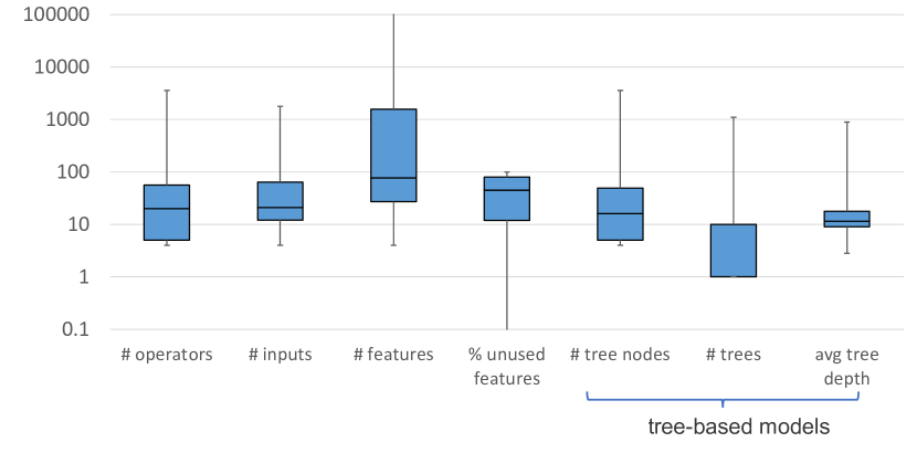
Figure 1. Statistics for ~$500$ traditional ML models in the OpenML CC-18 benchmark (OpenML, 2021). The boxplots represent the 25${}^{\textrm{th}}$, median, and 75${}^{\textrm{th}}$ percentile; the whiskers represent the min and max. Y-axis is in logscale.

2.1. Motivation

Inference drives the cost of ML in the enterprise. In most applications, models are trained at regular intervals but used for inference continuously. Although a training instance might be more costly than an inference one, inference ends up being significantly more costly than training on aggregate. Cloud vendors state that 90% of the total cost of ML is on inference (Jassy, 2021). Therefore, optimizing inference is crucial for lowering operational costs.

Batch inference is often preferable or at least sufficient. Online inference is not a requirement for most enterprise applications, especially after considering the infrastructure costs associated with it. In $130$ customer engagements at Microsoft, the requirements of $91\%$ of them were captured by batch inference. An additional $6\%$ (for a total of $97\%$) was managed with batch inference at short intervals. Hence our focus with Raven is on batch prediction queries.

Prediction queries in SQL. Input to Raven are prediction queries, i.e., advanced analytics queries that process data residing in (local or remote) files or databases through various data transformation operations and feed them into one or more trained pipelines. Two main ways are used to express such queries: SQL and Python. In this work, we consider the SQL syntax as adopted by SQL Server offerings (including Azure SQL DB and DW (Microsoft, 2021e)), i.e., a predict table-valued function (TVF) accepting as parameters a model (the trained pipeline) and a table, as depicted in Fig.  2 (➊). Similar SQL-based syntax is used by both Google BigQueryML (Google, 2021a) and Amazon RedshiftML (Amazon.com, 2021b), and recent work can be used to translate prediction queries from Python to SQL (Alekh Jindal, 2021).

Traditional ML is most widely used. According to the latest Kaggle survey (Kaggle, 2020) and an analysis of publicly available Python notebooks (Psallidas et al., 2019), traditional ML algorithms, such as linear/logistic regression and tree-based models (decision trees, random forests, gradient boosting) are the most popular by a large margin. ~$80\%$ of the Kaggle responders use them, as opposed to $43\%$ for neural networks. Scikit-learn (Pedregosa et al., 2011), which focuses on traditional ML, is the most widely used ML library in both studies. Thus, while Raven can execute queries including any model expressible in ONNX (ONNX, 2021a), our current focus is on optimizing queries with traditional ML operators.

Trained pipelines are complex and vary greatly. We studied $508$ scikit-learn trained pipelines over $72$ datasets from OpenML’s CC18 benchmark suite (Bischl et al., 2019). Fig.  1 highlights the significant variations across pipelines. Pipelines have a median of $21$ inputs but some receive more than $1000$ inputs. After featurization, due to categorical inputs, models have a median of $77$ features but some models have more than $50M$ features. Likewise, while most tree-based models (which account for $88\%$ of all models) include less than $10$ trees with a median depth of $11$, some are extremely complex with thousands of trees and depth. Each model consists of a large number of operators with an average of $126$, a median of $20$, and a min/max of $4$/$3560$, as shown in Fig.  1. Similar model complexity variations have been reported in production settings (Ahmed et al., 2019). These variations make different transformations be beneficial for each model and dictate data-driven optimization strategies to determine which rules to apply (§ 5).

Finally, to avoid overfitting in linear models, regularization techniques (e.g., Lasso) (Bishop, 2007) are often used during model training, which end up creating zero weights. In tree-based models, features are often left out during training due to correlations or insignificant contributions. In the $508$ OpenML models we analyzed, on average $46\%$ of the model features remain unused during inference! This observation makes the model-projection pushdown rule particularly effective, as we discuss in § 4.1.

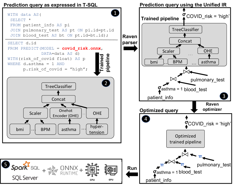
Figure 2. Prediction query using SQL Server’s predict statement ➊. It includes data processing operations (e.g., join, one-hot encoding) and invokes a trained pipeline ➋. Raven: ➌ constructs the corresponding intermediate representation (IR); ➍ optimizes the IR through cross-optimizations and transformations; and ➎ executes the final optimized plan using Apache Spark or SQL Server (depending on where the data is) and an ML runtime (if needed) over CPU or GPU.

2.2. Raven

Running example. Consider a model that predicts whether a patient is in high risk of COVID-19 complications. This model is trained over a large amount of data across several COVID-19 testing sites and hospitals. The result of model training is the model pipeline $M$, shown in Fig.  2 (➋). Along with the actual tree classifier, it includes pre-processing steps to prepare the data for inference. $M$ is deployed, and then a data analyst can use it in a prediction query $P$ to “find asthma patients who are likely in the high-risk COVID-19 group,” depicted in Fig.  2 (➊). The analyst uses $P$ to find such patients in a specific hospital and to do so, $P$ first joins patient_info with two test results (blood_test, pulmonary_test) and then invokes $M$. $P$ also includes filters on asthma and the result of $M$.

Building the unified IR. Given a prediction query $P$, which includes both data processing operators in SQL and the trained pipeline $M$, Raven parses $P$ and constructs a DAG expressed in Raven’s unified IR (Fig.  2 (➌)). The unified IR contains a mix of ML operators (the TreeClassifier, Scaler, and OneHotEncoder) and relational ones (e.g., the selection predicate over asthma and the joins between the three tables). The unified IR unlocks several logical and logical-to-physical optimizations.

Optimizations. Raven’s optimizer is a co-optimizer sitting alongside the optimizers of the data and ML engine, and is invoked before those optimizers. Given the IR corresponding to an inference query $P$, including both data and ML operators, the Raven optimizer triggers several optimization rules in the form of passes over the IR (Fig.  2 (➍)), falling in two main categories:

Logical optimizations that simplify the data part of the query by taking into account information from the ML part and vice versa (cross-optimizations) or that use data statistics to simplify the query (data-induced). Optimizations in this category are always beneficial and are applied first (similar to the heuristic optimizations always applied first by relational optimizers).

Logical-to-physical optimizations that transform traditional ML operators into equivalent SQL statements or neural networks to be executed by the data engine or the neural network runtime (possibly over GPU), respectively. Raven uses data-driven optimization strategies for determining which transformation to apply given $P$.

Note that well known optimizations are also triggered by the data and ML engines that Raven uses prior to executing $P$ (e.g., projection or aggregate pushdowns, join eliminations, compiler optimizations).

Execution of optimized plan. The final optimized prediction query will be executed by the data engine that owns the data (Fig.  2 (➎))—Apache Spark or SQL Server in our implementation. The data engine will perform all data operations (i.e., SQL operators, as well as ML operators that got translated to SQL by Raven) and will invoke ML runtimes as required for evaluating the trained pipelines. In particular, ONNX Runtime (Microsoft, 2021d) is integrated with SQL Server (Karanasos et al., 2020; Microsoft, 2021e) and can be invoked through the predict statement. We added a similar syntax in Apache Spark to invoke ONNX Runtime (both on CPU and GPU). More implementation details are discussed in § 6.

3. Raven’s Unified IR

IRs have been commonly used for optimizations in various settings. Most database optimizers rely on relational algebra (Ramakrishnan and Gehrke, 2003), whereas different IRs are used in ML runtimes (e.g., (Google, 2021c; ONNX, 2021a; Google, 2021b; Chen et al., 2018; Ragan-Kelley et al., 2013)) or to combine relational and linear algebra operators for ML training (Kunft et al., 2019; Hutchison et al., 2017). In Raven, we represent a wider range of data and ML operators in a unified IR, which allows us to perform logical optimizations holistically (§ 4) and perform runtime selection (§ 5). Our IR’s operators fall in the following categories:

• Relational algebra. This includes all the relational algebra operators, which are found in a typical RDBMS.

• Linear algebra. A large fraction of the operators used in ML frameworks, and in particular neural network runtimes (Abadi et al., 2016; Microsoft, 2021d; Paszke et al., 2019), fall into this category. Examples include matrix multiplication and convolution operators.

• Other ML operators and data featurizers. These are all the operators widely used in traditional ML frameworks (e.g., scikit-learn (Scikit-learn, 2021a), ML.NET (Ahmed et al., 2019)) but cannot be expressed in linear algebra. Examples are decision trees and featurization operations (e.g., categorical encoding, text featurization). Note that supporting such operators is crucial (see § 2.1) but also challenging, as they do not abide by an algebra and can correspond to arbitrary algorithms.

The main motivation when designing our IR was to (i) ease production adoption, and (ii) be able to express a wide range of prediction queries. To this end, we made the following design choices:

• We based our IR implementation on ONNX, which we extended with common relational operators (e.g., projections, selections), rather than start from a relational IR. This was a pragmatic choice as there are many more ML operators than relational ones.

• We chose ONNX for the ML part, as most popular frameworks translate to it. Our current set of ML operators is all ONNX operators, including featurizers (e.g., one-hot encoder, scaler, normalizer, etc.), linear algebra, and traditional ML ones (e.g., decision tree, random forest, gradient boosting, linear regression).

• Unlike most systems, we support more operators than just linear algebra for ML. Linear algebra is easily executed in the DB but lacks expressivity for models used extensively in production, e.g., featurizers and tree-based models.

Embracing widely used standards, namely SQL and ONNX, in our IR was key for production adoption. For example, on the relational side, all standard SQL operators in SQL Server and SparkSQL can be mapped to Raven IR operators. Similarly, on the ML side, by supporting ONNX, Raven also supports by transitivity all models that can be converted to ONNX (ONNX, 2021b), such as scikit-learn, SparkML, PyTorch, and TensorFlow. Given there is an 1-1 mapping between SQL/ONNX operators and our IR operators, it is also straightforward to construct the IR by traversing the prediction query.

Note that some operators are semantically very close, e.g., FeatureExtractor (common in ONNX graphs) and the relational Projection—we allow both in our IR and have equivalence rules that let us translate from one to the other. Models with operators that are not yet supported are executed but not optimized by Raven.

4. Logical Optimizations

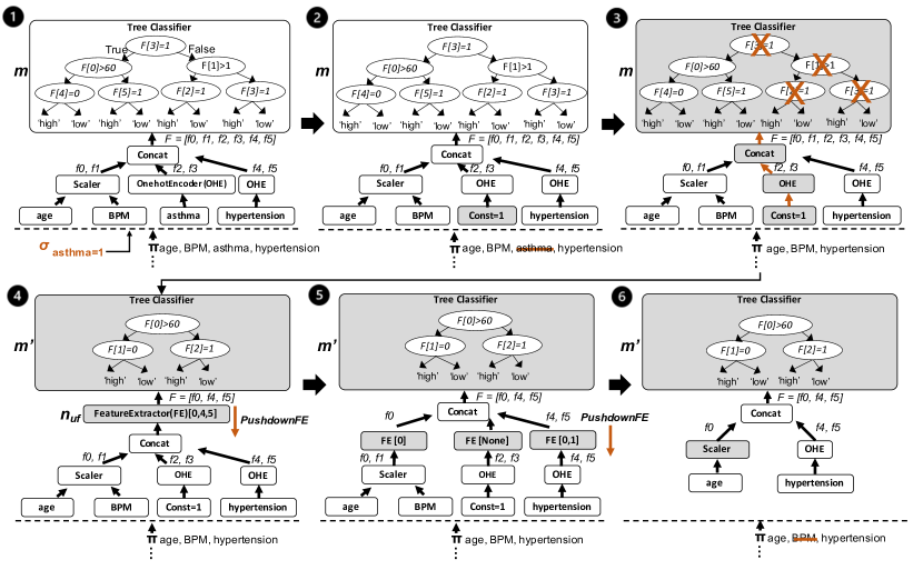
Figure 3. Cross-optimization steps for our running example (we omit some data operators from the IR): predicate-based model pruning (➊–➌) and model-projection pushdown (➍–➏). We use gray and orange to highlight the changes in the IR at each step.

In this section, we describe two types of logical optimizations applied by Raven’s optimizer: (i) cross-optimizations (§ 4.1) that exchange information between the data and ML parts of the query to optimize each other; and (ii) data-induced optimizations (§ 4.2) that exploit statistics of the underlying data to further simplify the query plan. All these are implemented as rules over Raven’s IR.

4.1. Cross-optimizations

In these optimizations, we leverage properties of the data processing part of the prediction query to optimize the ML part (data-to-model) and vice-versa (model-to-data). These optimizations can be seen as similar in spirit to sideways information passing at compile time (Beeri and Ramakrishnan, 1987). Below we describe one optimization from each category. Fig.  3 shows several versions of the IR when applying the two optimizations on the prediction query of Fig.  2 (➊).

We first introduced the two optimizations below in (Karanasos et al., 2020), supporting only models with a single linear regression or decision tree operator. We are expanding these optimizations here in two main ways: (i) we support a much wider range of traditional ML operators, including all common linear and tree-based models (decision trees, random forests, gradient boosting) and featurizers, covering all operators present in the hundreds of OpenML pipelines we studied in § 2 (for comparison, none of the OpenML operators were supported in (Karanasos et al., 2020)); and (ii) we support arbitrary ONNX models instead of single operators. A manual approach as in (Karanasos et al., 2020) could not handle this level of complexity: an actual optimizer is required to traverse the operator tree and apply the optimizations, propagating them through featurizers and other operators.

Predicate-based model pruning. Given a prediction query $P$, this data-to-model optimization identifies data predicates in $P$ (from the where clause of the query) and passes them to the trained pipelines in $P$ to simplify them, resulting in an optimized prediction query $P^{\prime}$. The benefit of this optimization is twofold: (i) it may reduce the number of inputs to the trained pipeline (if an input is a known constant, we do not need to provide it to trained pipeline at runtime); and (ii) it reduces the complexity of the models, e.g., by pruning tree-based models or statically pre-computing parts of the ML operations (e.g., multiplications in linear models).

For each trained pipeline $M$ of the query, the algorithm proceeds in two steps:

Step 1. It collects $M$’s inputs that participate in predicates. For each equality predicate, it replaces the corresponding model input with a constant node and adds a projection to prevent that input from reaching the model. This projection can then be pushed down by the relational optimizer to completely avoid scanning that column—with sufficient predicates even full table scans can be avoided. It also annotates with predicate information the model inputs corresponding to range predicates. In Fig.  3 (➋), given asthma=1, the algorithm replaces the asthma input with a constant node and removes the corresponding data column from the project operator.

Step 2. It passes the equality/range predicate information through the pre-processing/featurization operators of $M$ (e.g., Scaler, OneHotEncoder, Concat), updating the predicate information as needed. Once it reaches a tree-based model (e.g., decision tree, random forest, gradient boosting), it uses this information to prune branches of each tree in the model.

In Fig.  3 (➌), predicate asthma=1 becomes $[0,1]$ when pushed through the OneHotEncoder for the two categories [is_not_asthma_patient, is_asthma_patient]. Similarly, a constant $n_{c}$ is updated to $(constant-offset)\times scale$ when pushed through a Scaler. Moreover, TreeClassifier’s root and right branch were completely pruned based on asthma=1. It can also leverage range predicates, e.g., with age<30, it can further prune the right branch of the tree in Fig.  3 (➍).

Predicate-based model pruning can be particularly effective with predicates over a categorical input $c_{i}$ with $V$ unique values. These inputs are typically one-hot encoded to $V$ binary variables, and an equality predicate on $c_{i}$ leads to $V$ known constant model inputs.

We also support predicates on the outputs of the trained pipelines, such as risk_of_covid=’high’ in Fig.  2. In the case of tree-based models, we pick the leaves that satisfy the predicate and traverse the model bottom up, keeping the paths from these leaves to the model inputs and pruning all other nodes.

Model-projection pushdown. This model-to-data optimization relies on the model sparsity observation we made in § 2.1 about features often left unused during inference. Features might also be deemed unnecessary due to other optimizations: after predicate-based model pruning, the features of the right tree branch in Fig.  3 (➌) are no longer used. Model-projection pushdown identifies such unused features and attempts to push them down below the trained pipeline, towards the data processing part. This can bring significant performance benefits: (i) if we push the projection all the way to the scan, we completely avoid reading some features from disk; (ii) even if this is not possible, we might still be able to push them below joins, thereby significantly reducing shuffling costs, or avoid those joins altogether if all features of a table end up getting projected out.

This optimization is implemented as two passes over the IR, each applying a transformation rule until fixpoint. In the first pass, for each model $m$ in the trained pipeline $M$, it detects its unused features and creates a dense version $m^{\prime}$ of it. It then replaces $m$ with $m^{\prime}$ and projects out the unused features by adding a FeatureExtractor node $n_{uf}$ in $M$. In the second pass, a rule is triggered on every newly added $n_{uf}$ to push it down to its parents in $M$.

In Fig.  3 (➌), the original TreeClassifier using only the features with indices [0,4,5] is replaced by the densified model $m^{\prime}$ in Fig.  3 (➍) using indices [0,1,2] along with a FeatureExtractor node $n_{uf}$ to project out unused features from the model. In Fig.  3 (➎), the FeatureExtractor is pushed below Concat operator, creating three FeatureExtractors. The middle one is empty and is removed from the DAG along with its parents. The left-most is further pushed below Scaler, and the unused input BPM is removed from the pipeline and from the list of input columns in the Project operator (Fig.  3 (➏)).

Extension to neural networks. Based on the evidence data we presented in § 2.1, we have focused our efforts so far on traditional ML operators, such as linear and tree-based models and featurizers (see § 3), given their popularity. Thus, our optimizations cannot be applied to neural networks yet. Predicate-based model pruning in a neural network would amount to constant folding. Model-projection pushdown might be less beneficial on fully connected models like MLPs, but it remains open for sparser models.

4.2. Data-induced Optimizations

RDBMS as well as big data systems, such as Apache Spark, commonly store data statistics, such as maximum and minimum values for each data column, to allow the optimizer to generate better, more accurate query plans. Data statistics can also be used in concert with data partitioning to further speed up query execution, for instance by means of data skipping (Databricks, 2021).

In Raven, we make use of data statistics to optimize the ML models of a prediction query. For example, age is the root feature of the tree of Fig.  3 (➏), and any instance with age $>$ 60 will go in the left sub-tree of the tree, or right otherwise. However, if the input data contain no instance with age $\leq$ 60, the tree can be simplified by completely pruning the right sub-tree, also removing the participating data inputs (age in our example). Raven induces such predicates based on min/max data statistics.

Taking this idea a step further, we also exploit the fact that big data systems store data in partitions (Documentation, 2021), which are either specified by the user or are the result of a data operation (e.g., group-by). Following this intuition, Raven compiles an optimized model for each partition, leveraging the data distribution of that partition. Going back to our previous example, if data is partitioned and distributed over the age feature, Raven can generate partition-optimized trees by pruning the left or the right sub-tree based on the maximum and minimum value contained in each partition. Note that data-induced predicates can work with the other cross-optimizations: i.e., if a feature is pruned from a model thanks to a data-induced predicate, the model-projection pushdown optimization can further prune the column from the inputs if not used elsewhere.

5. Logical to Physical: Runtime Selection

We now focus on logical-to-physical optimizations that aim to convert (a set of) operator(s) to another in order to allow more efficient engines and hardware to be used for executing those operators (§ 5.1). A crucial observation is that such rules can be detrimental if not applied with care. For example, in our experiments, turning a scikit-learn gradient boosting classifier with default values ($100$ estimators, max-depth $3$) to a SQL statement led to a 6$\times$ slowdown. Therefore, we introduce three optimization strategies to judiciously pick when to apply each transformation (§ 5.2).

5.1. Transformations for Runtime Selection

MLtoSQL turns ML operators to SQL statements to avoid invoking the ML runtime for those operators, whereas MLtoDNN transforms traditional ML operators to equivalent (deep) neural networks (DNN) to make use of state-of-the-art DNN runtimes and compilers over modern hardware.

MLtoSQL. This optimization converts ML operators (linear algebra and other ML operators and featurizers; see § 3) to equivalent (i.e., semantics-preserving) relational ones. The main benefit of this conversion is to reduce or completely avoid (when we can convert the whole model pipeline to SQL) invoking the ML runtime, thereby avoiding initialization costs and data conversions/copies between the relational and ML engines. It can also enable more extensive relational optimizations in the DBMS, e.g., pushing ML computation (now expressed as relational operators) below joins and aggregates.

Raven supports the conversion of a wide range of traditional ML models to SQL, such as linear models (e.g., logistic/linear regression) and tree-based models, namely, decision trees, random forests, and popular gradient boosting models (LightGBM (Ke et al., 2017), XGBoost (Chen and Guestrin, 2016)). Furthermore, it supports representative featurizers: scalers, normalizers, and categorical feature encoders (e.g., OneHotEncoder, LabelEncoder).

The algorithm converts a model pipeline $M$ of a prediction query $P$ to an equivalent SQL statement. First, it replaces each ML operator in $M$ with a corresponding SQL operator. Linear models and scaling operators are converted to SQL using multiplication/addition/subtraction operators, while tree-based models and encoding operators are translated via case statements. For example, in case of decision trees, we do a depth-first search traversal of the tree nodes and create a nested case expression. For the TreeClassifier in Fig.  3 (➏), the corresponding SQL expression is:

CASE WHEN F[0] > 60 THEN (
  CASE WHEN F[1] = 0 THEN 1 ELSE 0 END) ELSE (
  CASE WHEN F[2] = 1 THEN 1 ELSE 0 END) END

Once the per-operator conversion is done, MLtoSQL traverses the updated IR in topological order and each SQL operator is merged with its parents to produce a single SQL statement out of the IR. MLtoSQL currently transforms the whole model pipeline $M$ to SQL or it fails (and $M$ is used instead). As part of our future work, we are investigating the benefit of a partial conversion.

Note that, as we discuss in § 5.2 and show in § 7, MLtoSQL should be used with care: it can be very beneficial in some cases but can be detrimental especially for complex models.

MLtoDNN. Unlike relational operators that are based on relational algebra and DNN operators that are based on tensor abstractions, traditional ML operators (i.e., non-DNN ones, such as featurizers and linear/tree-based models) do not follow a similar computation abstraction. Hence, despite its significance in the enterprise (as discussed in § 2), traditional ML has received less attention for optimization and hardware acceleration, as it is much harder to optimize arbitrary computation.

Raven leverages recent work on Hummingbird (Nakandala et al., 2020) to translate traditional ML operators to equivalent DNNs that can be executed on highly efficient DNN engines like ONNX Runtime, PyTorch, and TensorFlow. This is very important performance-wise, as DNN engines support out-of-the-box hardware acceleration through GPUs/FPGAs, as well as code generation (Chen et al., 2018). As we show in § 7, thanks to MLtoDNN, we were able to evaluate prediction queries on SQL Server and Spark using GPUs for the trained pipelines of the queries. Note that given the overhead of moving data to the GPU, we will show that complex models benefit more from this optimization.

We are also investigating similar translations for the relational operators, so that we can hardware accelerate them without having to implement custom GPU kernels.

5.2. Data-Driven Optimization Strategies

We now present novel optimization strategies that are employed by Raven’s optimizer to determine which optimization rules to apply on a given prediction query. We present an ML-informed rule-based and two ML-based strategies.

The input prediction query $P$ might include one or more predict operators, each invoking a trained pipeline (see § 2). Raven triggers the optimization strategy on each sub-part of the IR that corresponds to a predict statement. In our running example, this is the part of the IR that corresponds to the trained pipeline $M$, depicted in the gray box in Fig.  2 (➋).

To perform data-driven decisions, we used the OpenML CC18 classification benchmark (Bischl et al., 2019) we described in § 2.1. We used $138$ models, which we executed using all combinations of our rules (both on CPU and GPU in the case of MLtoDNN). All OpenML evaluations were performed on Azure NC12s_v2 instances, each with $12$ vCPUs, $224GB$ of RAM, and an NVIDIA Tesla P100 GPU.

Our first observation is that our logical optimizations (§ 4) are always beneficial, as they reduce the required computation and data inputs when applicable, or leave the prediction query unchanged otherwise. Therefore, Raven applies them in all cases. This intuition was confirmed in all OpenML runs. The resulting speedup from these optimizations depends on the number of data predicates and unused columns, as we show in § 7. We apply the predicate-based model pruning before model-projection pushdown, as the former can enable further application of the latter (see § 4).

On the other hand, our OpenML runs showed that the impact of each logical-to-physical optimization (§ 5.1) varies, as also shown in § 7.2. Therefore, the optimization strategy has to choose between four evaluations for the trained pipeline: MLtoSQL (using the relational engine), MLtoDNN (evaluating the resulting DNN on CPU or GPU), or none of them (using the ML runtime after applying only the cross-optimizations). Based on our runs, we excluded MLtoDNN-on-CPU from the choices when a GPU is available, as it always gave worse or similar performance to MLtoDNN-on-GPU. Next we introduce different optimization strategies to pick between the above three evaluations based on the model’s characteristics.

ML-informed rule-based strategy. Instead of hard-coding rules based on experience and magic numbers (like existing relational optimizers often do), this strategy follows a hybrid approach. It trains a decision tree based on our OpenML runs, uses it to find the $k$ most contributing features, and uses those to build a new much shallower decision tree that is turned to a rule. This also allows us to adapt to the specific hardware in hand. For each of the $138$ trained pipelines in the benchmark, we gathered $22$ statistics, including: #inputs to the pipeline; #inputs to model (after featurization); #specific operators (e.g., one-hot encoders/OHEs); mean/max #outputs of OHEs; #trees, mean/max/stddev tree depth for tree-based models. As an example, using $k=3$ to strike a balance between simplicity and accuracy, the following rule was generated: if #features $>$$100$, apply MLtoDNN; else if #inputs $>$$12$ and mean tree depth $\leq$$10$, apply MLtoSQL. The added benefit of this strategy is that no ML model needs to be invoked during optimization, which makes deployment in production simpler.

Classification-based strategy. In this strategy, we train an ML classifier using the OpenML dataset with the $138$ trained pipelines and the $22$ features mentioned in the rule-based strategy. The classifier predicts one of the following classes that correspond to the transformation to be applied: MLtoSQL, MLtoDNN, none. We experimented with several scikit-learn (Scikit-learn, 2021a) classifiers (using default values), such as logistic regression, decision tree, random forest, and gradient boosting. Out of them, we use the random forest, as it gave best accuracy results.

Regression-based strategy. In this ML-based strategy, instead of building a classifier to directly pick the most promising transformation rule, we build a regression model that predicts the expected runtime after applying one of the MLtoSQL, MLtoDNN, and no transformation variants. Therefore, the transformation becomes a feature in the regression model. The benefit of this approach is a 3-fold increase of the training set (one fold for every transformation option). At inference time, we perform three predictions, one for each transformation, and pick the option that gives the lowest runtime. We experimented with several scikit-learn regression models (e.g., linear regression, decision tree, random forest, XGB, adaptive boosting), and opted again for the decision tree due to best accuracy.

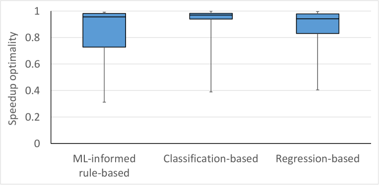
Figure 4. Inference time speedup over optimal strategy achieved by different optimization strategies. Reported numbers are over $200$ stratified folds of the OpenML training dataset. Boxplots indicate 25${}^{\textrm{th}}$, median, and 75${}^{\textrm{th}}$ percentile; whiskers indicate min and max values.

Strategy evaluation. We now compare the performance of our strategies on the OpenML benchmark. Given our training set is relatively small and imbalanced ($25$ models perform best with MLtoSQL; $72$ with MLtoDNN; $41$ with no transformation), we use stratified $5$-fold cross validation (with an 80/20 split between the training and test sets) and repeat the process $40$ times for a total of $200$ runs. The rule-based had the lowest mean accuracy ($0.76$), while the ML-based ones both had $0.79$ (the regression-based had higher accuracy variance). Fig.  4 depicts the speedup achieved by each strategy (considering the total inference time to run all models of a run’s test set) when compared to using the optimal transformation for each model. The median speedup of all three is comparable (classification-based is best with a speedup of $0.97$). However, classification-based has significantly lower variance, e.g., its $25^{\textrm{th}}$ percentile speedup is $0.94$ as opposed to $0.72$ and $0.83$ for the rule- and regression-based, respectively. In terms of training time, the $200$ runs took less than a minute for each strategy—users can go through this process once to finetune the strategy on their workload and hardware setup.

To sum up, Raven first applies the logical optimizations in a strict order (predicate-based pruning before model-projection pushdown), and then it applies the logical-to-physical ones based on our data-driven strategies. Among the ML-based strategies, the classification-based is preferable. The rule-based is a viable alternative when it is not desirable to invoke ML models during optimization.

6. Implementation

We implemented Raven as an extension to Apache Spark, depicted in Fig.  5 with the main Raven components in gray. In particular: (i) we introduced the predict statement to allow SparkSQL users to express prediction queries, similar to (Microsoft, 2021e; Google, 2021a; Amazon.com, 2021b); (ii) we added a new rule to the Catalyst optimizer that internally invokes our Raven optimizer, described in § 5.2; and (iii) we defined a Python UDF that allows invoking external ML runtimes (ONNX Runtime in the current implementation, as we support ONNX and ONNX-convertible models) to execute the prediction queries (on CPU and GPU). In our integration, we made heavy use of Spark’s extensibility framework: Raven is provided as an external jar and no modification to Spark’s source code is required. This was required to be able to deploy Raven in any existing Spark installation and across Microsoft’s Spark offerings. The predict statement was made publicly available recently as part of our Azure Synapse Spark offering (Microsoft, 2021g); we are actively working on productizing the optimizer, too.

Raven can be enabled programmatically by invoking the Raven ​Session instead of the usual SparkSession. Below we present the main components introduced, and then discuss how Raven can generate queries to be executed in SQL Server.

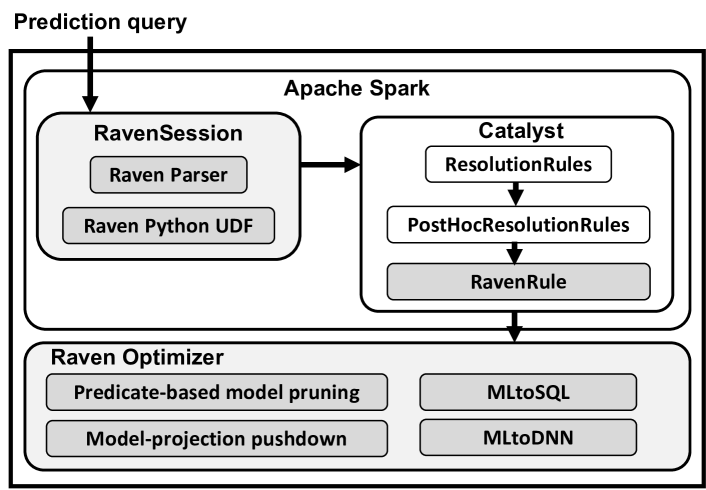
Figure 5. Raven integration in Spark with the newly introduced components shown in gray.

Adding the predict statement to the parser. We extended the ParserInterface to allow users to submit SparkSQL queries containing predict statements either as (i) a UDF, e.g., select predict(model.onnx, *) as predict from table; or (ii) as a table-valued function (TVF), e.g., select data.*, prediction.score from predict(model = model.onnx, data = data) with(score float) as prediction). We internally rewrite predict TVFs into UDFs, so that we can have a single implementation for execution. The Raven parser detects predict statements and rewrites them to call the pre-defined Raven Python UDF we introduced to invoke ML runtimes (see below). This allows us to hide the details of the Raven UDF from the users and to trigger the Raven optimizer when a predict statement is detected.

Optimizing SparkSQL prediction queries. We introduced a single PostHocResolutionRule (“Raven ​Rule” in Fig.  5) to trigger the Raven (co-)optimizer when a predict statement is detected. This rule calls the Raven optimizer as an external Python process. It also provides the optimizer with the predicates in the where clause of the query (for the predicate-based model pruning rule), along with the model filename.

The Raven optimizer uses the onnxconverter_common library (ONNX, 2021b) to build a DAG of ONNX operators, containing all ML operators (see § 3) present in the prediction query. The data operators of the query are then added to the IR. Once the full IR is built, the optimizer triggers all rules. The output is the filename of the optimized model and a (possibly empty) set of columns (output of the model-project pushdown rule). The rule then injects a new Projection operator, and rewrites the predict with the new model information.

To deal with the wide range of ONNX operators, we strive to share rule implementations across operators when possible. In particular, we share most of the rule implementation within linear models and within tree-based models (e.g., forests are just multiple trees). Featurizers are trickier and we tend to have custom code for each.

Running predictions with the Python Vectorized UDF. We implemented the Raven UDF using Spark’s Python vectorized UDF (Spark, 2021), which allows to execute arbitrary Python code on a columnar view of input data, given as batches (of 10k tuples by default). Our UDF implementation performs the following: (i) loads the model from HDFS; (ii) initializes and caches the model on a global variable to decrease model loading overheads in successive invocations on the same worker; (iii) transforms the input columns to the right format; and (iv) invokes ONNX Runtime to perform the prediction.

Regarding the translation between relational data and model inputs (step (iii) above), most traditional ML models that we consider receive vectors as inputs (M$\times$1, with M being the batch dimension). Spark’s vectorized UDF automatically turns data to columnar Pandas dataframes, hence the translation is a 1-1 mapping. For models with M$\times$N inputs, we concatenate the M$\times$1 vectors within the UDF.

Transforming Raven plans to SQL Server queries. If specified by the user, Raven can output a T-SQL version (SQL Server’s SQL dialect) of the optimized prediction query. Our goal with this design is to enable Raven to output queries for other DBMSs too.

7. Experimental Evaluation

We now evaluate the benefits of Raven on prediction queries over real-world datasets. To this end, we use Raven to optimize the queries and execute them on Apache Spark and SQL Server (see § 6). We compare our results with several state-of-the-art systems for evaluating prediction queries, namely, SparkML, Spark invoking scikit-learn and ONNX Runtime, as well as MADlib (§ 7.1). Then, through a set of micro-experiments, we study the impact of each optimization rule on various model types (§ 7.2) and the benefit of GPU acceleration (§ 7.3). We finally include a discussion on overheads, coverage, and accuracy. Our key results are the following:

• On Spark, Raven with all optimizations enabled delivers speedups of 1.4–13.1$\times$ against Raven with no optimizations, and up to 48$\times$ and 25.3$\times$ speedups against SparkML and Spark with scikit-learn, respectively.

• On SQL Server, Raven plans provide speedups of 1.4–330$\times$ over plans without Raven optimizations. Single-threaded Raven gives speedups up to 108$\times$ over MADlib for the supported queries.

• For complex models, such as large gradient boosting models, Raven can deliver significant speedups over GPUs: up to 8$\times$ on Spark and 2.6$\times$ on SQL Server.

• Based on the characteristics of each prediction query, different optimizations lead to optimal performance (as also shown in our optimization strategies of § 5).

Table 1. Summary of dataset statistics

Datasets	# of tables	# of data inputs (numeric /categorical)	# of features after encoding (numeric/categ.)
Credit Card (Kaggle, 2021)	1	28 (28/0)	28 (28/0)
Hospital (Microsoft, 2021f)	1	24 (9/15)	59 (9/50)
Expedia (Project Hamlet, 2021)	3	28 (8/20)	3965 (8/3957)
Flights (Project Hamlet, 2021)	4	37 (4/33)	6475 (4/6471)

Datasets. Throughout our experiments, we use four real-world datasets that have been widely used in data science tasks (Kaggle, 2021; Project Hamlet, 2021; Microsoft, 2021f), summarized in Tab.  1. Some datasets are comprised of a single table while others of multiple ones, allowing us to vary the complexity of data operations from simple scans to multi-way joins. The datasets include both numerical and categorical columns—the number of features per dataset (after encoding) ranges from 28 to 6,475 features. In order to test prediction queries at scale and to match the dataset sizes we observe in production, we replicate each dataset several folds, while making sure to not violate any primary-key constraints—for each experiment, we will specify the scale used.

Trained pipelines. We evaluate Raven over four popular traditional ML model types (Psallidas et al., 2019; Kaggle, 2020), namely, logistic regression (LR), decision tree (DT), gradient boosting (GB), and random forest (RF). Each trained pipeline includes featurizers for numerical and categorical inputs: we normalize the former using standard scaling, and encode the latter using one-hot encoding (Scikit-learn, 2021c, b). Trained pipelines all implement a binary classification task. Each pipeline is trained using scikit-learn over 80% of the original (not scaled) datasets, and then converted into the ONNX format. Each operator of the pipeline is trained using its default hyperparameters setting except when stated otherwise.

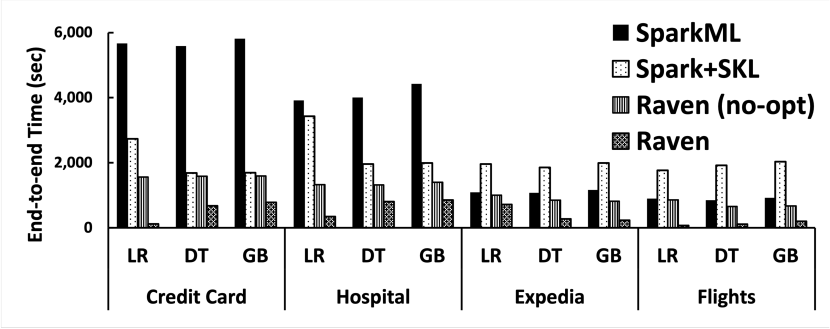
Figure 6. Prediction query runtime on Spark for different models and datasets, comparing Raven with: SparkML, Spark with scikit-learn, and Raven w/o optimizations.

Prediction queries. The prediction queries we use over single-table datasets (i.e., Credit Card and Hospital) involve a single table scan, whereas queries over Expedia and Flights involve a 3-way and a 4-way join, respectively. For the extra data predicates (e.g., asthma=1 in our running example), we add equality predicates in the where clause of the queries.

Reported metrics. For each experiment we report the trimmed mean of the execution time of five runs, removing the lowest and highest runtimes. For the Spark experiments, we report the total amount of time it takes to execute the prediction query and write the result to HDFS (with df.write.parquet(hdfs://...)) to avoid moving all results to the driver node. For SQL Server we add an aggregate operator on prediction results on the prediction queries.

System setup. For our Spark experiments, we set up a Spark v2.4.4 cluster on Microsoft Azure HDInsight (Microsoft, 2021b). It runs on YARN with 4 worker nodes and a driver node. Each worker has 56GB RAM and 8 cores, and the driver has 28GB RAM and 4 cores. We store data in Parquet (Parquet, 2021) on Azure Block File System (ABFS). We leave the UDF batch size fixed at the default 10k rows per batch. For SQL Server, unless otherwise specified, we used an Azure D32ds_v4 VM instance, with 32 vCPUs, 128GB of RAM, and a 1.2TB SSD. We used the clustered columnstore index for all database tables. For MADlib, we used version 1.17.0 on PostgreSQL 10.15.

Trained pipelines are authored using scikit-learn 0.21.3 (we use this version in inference comparisons, too). We use ONNX Runtime 1.2.0 and Hummingbird 0.2.1 (which internally uses PyTorch 1.7.1).

7.1. End-to-end Raven Evaluation

In this section, we evaluate Raven against state-of-the-art frameworks, both distributed on Apache Spark (§ 7.1.1) and single-node on SQL Server (§ 7.1.2). These experiments are on CPUs. We use the classification-based optimization strategy, as it gave us the best results (see § 5.2).

7.1.1. Raven on Spark

We compare our Raven implementation on Spark (which uses ONNX Runtime as its ML runtime—see § 6) against Raven with all optimizations disabled (Raven (no-opt)) and the following widely used alternatives for distributed inference: (i) SparkML; and (ii) a UDF-based approach similar to Raven (no-opt) but with scikit-learn as its ML runtime (Spark+SKL), to make sure Raven (no-opt) is competitive with state-of-the-art approaches.

Datasets. Credit Card is scaled to 1.6B rows; Hospital is scaled to 2B rows; Expedia is scaled to 500M rows; and Flights is scaled to 200M rows. We use a varying Hospital dataset size in the scalability experiment below. We use (uncompressed) datasets between 200MB (1M rows Hospital dataset) and 800GB (Credit Card). This scaling aligns with our customer needs: most production datasets we see are between 1GB and 1TB.

Prediction queries. For this experiment we pick three models: DT with max tree-depth of 8; LR with L₁-regularization and $\alpha$ (the regularization strength) set to 0.001; and GB with 20 estimators and max-depth of 3. These models have, across all datasets, higher or similar AUC than the ones trained with default scikit-learn hyperparameters. In § 7.2 we study Raven’s performance using different model parameters. We implemented SparkML queries using PySpark with the same operators and settings as the scikit-learn pipelines. Prediction queries in this experiment are run without data predicates.

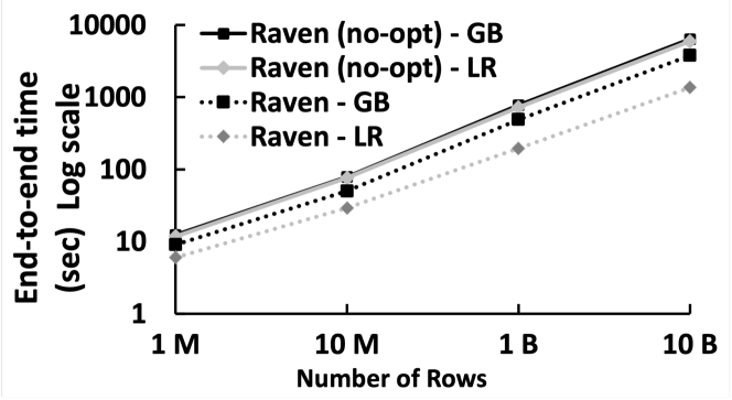
Figure 7. Performance of Raven (with and without optimizations) for increasing Hospital dataset size.

Comparison with other systems. The results for this experiment are reported in Fig.  6. Raven delivers 1.4–13.1$\times$ speedup compared to Raven (no-opt). Simpler models such as LR and DT benefit from both model-projection pushdown and MLtoSQL optimizations, avoiding reading unnecessary data by pruning unused data inputs and avoiding invoking ONNX Runtime (as the whole query is translated to SQL). This leads to a performance improvement of up to 13.1$\times$. Even when the optimizer selects no transformation rule, queries still benefit from Raven’s cross optimizations (i.e., model-projection pushdown—see details in § 7.2.2). More interestingly, for Expedia and Flights (using 3-way, 4-way joins respectively), Raven is able to push the projections on the unused inputs below joins, saving a lot of data movement and compute cost. Note that MLtoDNN is not beneficial for any of those queries, and in fact it is never picked by the optimizer. As we will show later, more complex queries on GPUs make use of it.

Our results also show that Raven is faster than the other frameworks, often by a large margin. SparkML is significantly slower than Raven—between 1.5 and 48$\times$. Compared to Spark+SKL, Raven is 2.15–25.3$\times$ faster. For single-table datasets, SparkML is slower than Spark+SKL and Raven (no-opt), but it is faster than Spark+SKL and comparable to Raven (no-opt) when joins are involved.

Data scalability. To study Raven’s scalability with increasing data size, we picked LR and GB from the above models (as Raven triggers different optimizations for each of them) and compare Raven with Raven (no-opt) for the hospital dataset with sizes of 1M to 10B tuples. Fig.  7 shows that Raven consistently outperforms Raven (no-opt) for all models and dataset sizes: by 1.96–4.36$\times$ for LR and by 1.37–1.67$\times$ for GB. Raven scales super-linearly to the data size, and this is likely due to the fact that for the small scales the cluster resources are not fully utilized.

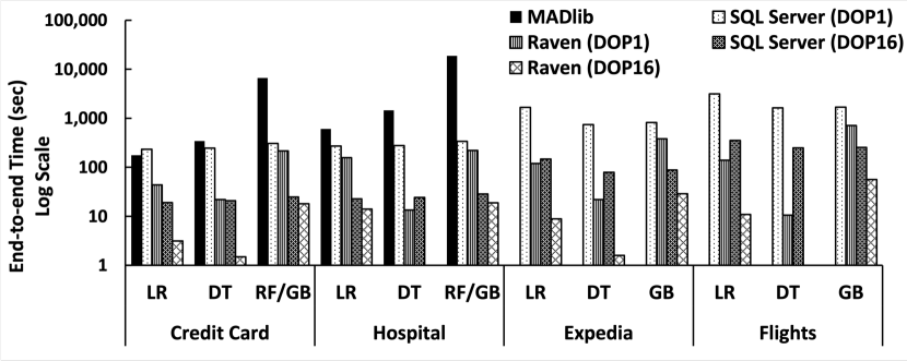
Figure 8. Prediction query runtime on SQL Server, both unoptimized and optimized by Raven for degree-of-parallelism (DOP) 1 and 16, and on PostgreSQL with MADlib.

Figure 9. Impact of optimizations on linear models for the Credit Card dataset with varying regularization strengths $\alpha$.

Figure 10. Impact of optimizations on decision trees for the Hospital dataset with varying tree depths.

Figure 11. Impact of data-induced optimizations on decision trees for the Hospital dataset with two partitioning schemes.

7.1.2. Raven on SQL Server

Here we configure Raven to output SQL Server queries (see § 6) and compare them with the original unoptimized queries on SQL Server. In both the optimized and non-optimized case we use SQL Server’s predict statement that invokes ONNX Runtime to evaluate the model pipelines (Microsoft, 2021e; Karanasos et al., 2020) along with all default SQL Server optimizations enabled. We also compare against MADlib (on PostgreSQL), which is another well-known in-database ML engine (Hellerstein et al., 2012). Since MADlib supports only single-threaded execution, for a fair comparison we report both single-threaded (with degree-of-parallelism 1 or DOP1) and multi-threaded (DOP16) execution for SQL Server (and thus Raven). Unlike SQL Server, PostgreSQL does not support a columnstore layout.

Datasets scale. We use all four datasets scaled to 100M rows.

Prediction queries. We use the same queries as in § 7.1.1 with the exception of the GB model in MADlib which we substitute with RF as this is the only tree ensemble model supported by MADlib. For the MADlib queries, we trained models using MADlib’s ML training libraries with the same hyperparameters used for the original models. Note that MADlib does not support pipelining of ML operations in most cases—instead we were forced to materialize the output of the featurization. For Expedia and Flights this led to surpassing the max number (1,600) of columns PostgreSQL allows in a table. Therefore, we skip these two datasets in the MADlib experiments.

Results. Fig.  8 shows the results of our runs for Raven on SQL Server, (un-optimized) SQL Server, and MADlib. As discussed in § 7.1.1, Raven triggers model-projection pushdown for all models, but MLtoSQL only for LR and DT. Over SQL Server, it delivers speedups of 1.4–330$\times$. Specifically for DOP16, for LR and DT models, Raven outperforms SQL Server by up to three orders of magnitude due to the translation to SQL and the removal of unused inputs, which are further pushed down below joins by SQL Server’s optimizer. Moreover, for the cases that the whole query gets translated to SQL, Raven benefits from multi-threading more than the un-optimized query on SQL Server does. The bigger speedup in the SQL Server experiments compared to the Spark ones is due to SQL Server’s more sophisticated optimizer. When Raven turns a model to a SQL statement with ML-to-SQL, SQL Server can optimize it much more than Spark. Finally, single-threaded Raven significantly outperforms MADlib by 3.9–108$\times$. This is to a large extent due to MADlib’s materialization of intermediate featurization steps and its lack of Raven optimizations.

7.2. Micro-experiments

In this section, we explore the impact of each optimization rule (see § 4) on different model types.

7.2.1. Linear Models

We first study the benefits of Raven’s optimizations as we increase the sparsity of the linear model. To this end, we use the Credit Card dataset with 200M rows on LR models with varying $L_{1}$-regularization strengths ($\alpha$ parameter). The lower the value of $\alpha$ the higher the regularization strength and the less the features with non-zero weights.

Our results are given in Fig.  11. The X-axis shows the $\alpha$ value and the resulting number of zero-weight inputs (out of the 28 total inputs). We report runtimes for different combination of rules (we use ModelProj to denote model-projection pushdown) and for Raven (no-opt) with all optimizations disabled.

We see that the combination of ModelProj and MLtoSQL is the best optimization for all LR model variants. Using only one of the two is not sufficient for realizing the full benefits of Raven. ModelProj shows that as $\alpha$ increases, this optimization varies from only taking 20% of the baseline run-time (with $\alpha$ = 0.001) to requiring slightly longer than the baseline (with $\alpha$ = 2), as the number of unused features decreases and thus the amount of data to be read increases. MLtoSQL alone is consistently about 60% of the baseline run-time, as it avoids invoking the ML runtime. The LR models in this experiments do not require too much compute, and therefore translation to DNN is not beneficial.

7.2.2. Tree-based Models

In this section, we evaluate Raven’s optimizations over decision trees. All experiments in this section were run on the Hospital dataset with 200M rows.

Model complexity. In Fig.  11 we show the impact of Raven’s optimizations as we increase DT’s depth. The X-axis depicts the tree depth and (in parentheses) the number of columns, out of the 24, that are not used by the DT—the higher the depth the more inputs participate. As we can see, model-projection pushdown is less effective as the tree depth increases, because less inputs are unused and can be pruned.

MLtoSQL provides a 21.7$\times$ speedup for the depth-3 tree, but gets progressively less beneficial as tree depth increases, becoming a 2.3$\times$ slowdown for the final model. Note that the performance of MLtoSQL alone varies for tree models, whereas its impact on all LR models in Fig.  11 was the same. This is because, unlike MLtoSQL for LR, MLtoSQL for DT is automatically pruning unused features even without ModelProj—it creates case statements (see § 5.1) only for paths with used inputs and the relational optimizer automatically projects out the rest. This is also the reason that ModelProj does not provide additional benefit on top of MLtoSQL. Finally, as with LR, MLtoDNN is not a good option for small DTs on a CPU cluster.

These results reinforce the importance of optimization strategies for picking the most efficient runtime, as shown in § 5.2.

Data predicates. In this experiment, we study the benefit of the predicate-based model pruning optimization by introducing an equality predicate in the where clause of the prediction query for the Hospital dataset. We experimented with different DT models. For the decision tree with depth 20, which uses all 24 inputs, this optimization allowed to prune several tree branches based on the equality predicate. This led to an optimized trained pipeline with a shallower tree (i.e., depth 15) along with less data inputs (i.e., 23 inputs). Raven saved $\sim$8% of query time with predicate-based model pruning, and additional $\sim$12% by removing 2 more data inputs with model-projection pushdown.

Table 2. Columns pruned by the data-induced optimization for three decision tree models on the Hospital dataset with different data partitioning schemes.

Decision tree depth	average # of pruned columns
	no partitioning	partitioning on num_issues	partitioning on rcount
10	4	8	11
15	0	6	5
20	0	6	5

Data-induced optimizations. To assess the benefit of the data-induced optimizations (§ 4.2), we use the Hospital dataset, which we now partition in two different ways—on the ‘number of health issues’ column (num_issues) and the ‘readmission count’ column (rcount), respectively. The former led to two partitions (whether or not there were health issues), while the latter led to six partitions.

Raven uses the data-induced predicates to generate a different optimized (stripped-down) model for each partition. We compare: (i) Raven (no-opt); (ii) Raven w/o partitioning, which is the “best-of” our prior optimizations (when data is not partitioned, the data-induced optimization is not applied); and (iii) Raven on the two partitioned versions of the dataset with all optimizations enabled. Fig.  11 shows the impact of the data-induced optimizations on the end-to-end time of scoring 200M rows of the Hospital dataset for decision trees of varying depth, while Tab.  2 shows the number of columns that were pruned on average across the optimized models. For decision trees with depth 15 and 20, Raven with the data-induced optimization improves the performance by $\sim$20% due to the additional tree pruning based on the induced predicates (see Tab.  2) whereas Raven w/o partitioning is similar to Raven (no-opt). For depth 10, Raven with partitioning provides 2.1–3.2$\times$ and 1.3–2.1$\times$ performance improvements over Raven (no-opt) and Raven w/o partitioning, respectively, due to pruning more tree branches along with the MLtoSQL transformation. Although the exact benefit depends on the partitioning column, it is beneficial in both cases.

Figure 12. Impact of MLtoDNN rule over CPU and GPU on complex gradient boosting models for the Hospital dataset.

7.3. GPU acceleration of complex models

Although we showed that MLtoDNN is not beneficial for simple models, using GPUs can greatly decrease inference time for more complicated ones, which are not uncommon as we saw in § 2. For this experiment, we used a separate Spark cluster with one driver node and three worker nodes, each with 6 CPUs, 56 GB memory, and NVIDIA Tesla K80 GPUs. We purposely picked this setup to have an hourly cost close to the CPU Spark cluster we used.

Unlike § 7.1 where we used 20 estimators with max tree-depth 3, here we use 60–500 estimators with max depth 4–8. For these models, model-projection pushdown is not beneficial as all inputs are used, and MLtoSQL is detrimental as it generates too complex SQL expressions.

Fig.  12 shows our results to compare Raven without optimizations with Raven that triggers MLtoDNN. The resulting plan includes a PyTorch DNN (instead of the original GB model) that we execute over both CPU and GPU (the remainder of the plan is executed on CPU) for the Hospital dataset. We observe speedups of 1.56–7.96$\times$ on GPU. Note the break in the graph: the 500 estimators/depth 8 model took 3,184 seconds on CPU without optimizations and only 400 seconds when run on GPU. In general, the more complicated the model, the bigger the speedups on GPU. Depending on the complexity of the model, MLtoDNN can be beneficial on CPU, too: the first two models have a minimal slowdown due to overhead, but the rightmost models have sizable speedups of 1.08–1.33$\times$ on CPU.

We performed the same experiments for SQL Server on an Azure NC6s_v3 instance with a Tesla V100-PCIE-16GB GPU. MLtoDNN produced speedups of 2.3–2.6$\times$ across the four models. For these runs we use SQL Server’s Python extensibility framework (Microsoft, 2021a)—using a tighter integration (Microsoft, 2021e) should further increase benefits.

7.4. Discussion

Optimization overheads in Spark. Our (un-optimized) inference queries on Spark showed an overhead of 2–4 seconds for cold runs and $\sim$0.1 second on warm runs, related to invoking the ML runtime through the Python UDF and loading the model from HDFS. Although optimization time varies based on model type and dataset, model-projection pushdown takes 1–5 seconds, MLtoSQL takes 3–5 seconds, and MLtoDNN takes 0.1–0.5 seconds on warm runs. Among our experimental prediction queries, the complex ones with hundreds of nodes in the IR tend to take up to 5 seconds for optimizations. On our four-node Spark cluster, we found that $\sim$1M rows were a sufficient quantity across all of our datasets to mask the optimization overheads (see Fig.  7). We are investigating optimizations that could further reduce these overheads. Moreover, some of our optimizations could be performed offline (saving the optimized model/plan)—this way Raven can be beneficial for any dataset size.

The main overheads introduced by the predict statement are from (i) the model loading from disk, (ii) the startup time for the UDF (i.e., the Python runtime startup cost), and (iii) the data conversion from Spark internal row representation to the format used by the models. For (i), we are already exploring how to cache/reuse models within Spark. For (ii), an alternative is to implement the UDF directly in Scala. However, this will force us to call the ML runtime using JNI, which will introduce other overheads. For (iii), when calling a predict UDF, Spark converts its row format to Arrow and then to Pandas dataframes. Most overhead comes from the conversion to Arrow, while the Arrow-to-Pandas conversion is zero-copy.

Coverage. To study the coverage that our IR and our optimizations provide in terms of ML operators, we trained 508 scikit-learn pipelines from the OpenML CC-18 benchmark (Bischl et al., 2019), which we converted to ONNX. We found that all operators can be expressed in our IR. Regarding the applicability of Raven’s optimizations, model-projection pushdown can be performed on all pipelines, MLtoSQL lacks support for just $4$ operators across all pipelines, and MLtoDNN covers 88% of all pipelines.

Prediction accuracy. To investigate whether our operator transformations (§ 5.1) introduce rounding errors, we compared the result of the optimized Raven plan with the unoptimized one for all our models in Spark and SQL Server. In the 30 models that we examined, MLtoSQL led to rounding errors in $0.006$–$0.3$% of the predictions, whereas MLtoDNN in less than $0.8$% (Nakandala et al., 2020). Such negligible rounding errors are considered acceptable for ML converters (ONNX, 2021b).

8. Related Work

The history of integrating ML algorithms in databases is rather long. In the early 2000’s, SQL Server shipped with data mining operators (Netz et al., 2000). Later in the 2010’s, MADlib (Hellerstein et al., 2012) suggested using UDAs/UDFs for embedding ML into the database. Apache Spark’s MLlib (Meng et al., 2016), Apache Mahout Samsara (Schelter et al., 2016) and others (Sparks et al., 2013; Sparks et al., 2017; Feng et al., 2012; Kumar et al., 2015; Jasny et al., 2020; Schüle et al., 2019; Zhang et al., 2021) can be seen as a continuation of this effort. A broad overview of in-DB ML techniques can be found in (Kumar et al., 2017). All these works, however, focus mostly on the training aspect of ML that is heavy on iterations. Moreover, ML components are handled as black boxes, thereby limiting optimization opportunities.

More recently, Amazon, Google, and Microsoft have added support for in-DB ML inference (Microsoft, 2021e; Karanasos et al., 2020; Google, 2021a; Amazon.com, 2021b), also focusing on enterprise capabilities of managed databases (Agrawal et al., 2020). Raven follows the architectural trend of collocating data engines with ML runtimes for inference, and takes it a step further by co-optimizing relational and ML operators and using the most efficient runtime for each part of the prediction query. As part of our broader effort to make it easier to author inference queries using any model, we have made the predict statement available in several of our engines, including Azure Synapse SQL and Spark, and Azure SQL Edge (Microsoft, 2021e, g, c).

The Raven optimizer we presented in this paper realizes and extends the vision that we first introduced in (Karanasos et al., 2020) in the following ways: we (i) built an end-to-end optimizer for applying the logical optimizations, (ii) added the data-induced optimizations, (iii) introduced data-driven strategies for the logical-to-physical optimizations, (iv) provided several production evidence data, the OpenML study, and (v) an extended experimental evaluation. Our initial prototype of (Karanasos et al., 2020) could manually apply just two logical optimizations over single-operator linear regression and decision tree models, but real models include at least tens and up to thousands of operators. The optimizer we presented here covers all OpenML pipelines for the logical optimizations and 88% for the physical ones—our initial prototype could handle none of these models.

SystemML explores cross-optimizations between relational and ML operators, but, unlike Raven, focuses on the training part. Probabilistic predicates (Lu et al., 2018) is a method to learn predicates and push them below trained pipelines for optimizing inference—such techniques could be integrated with Raven, too. More recently, (Kang et al., 2020) co-optimizes featurization and deep learning models. Thanks to its whitebox approach, Raven is able to optimize arbitrary ML pipelines containing featurizers, trees, and algebraic models.

Tensorflow’s tf.data (Murray et al., 2021) provides optimizations for data pipelines feeding Tensorflow models, but no cross-optimizations between data and ML are explored. Teradata’s recent Collaborative Optimizer (Eltabakh et al., 2021) pushes projections and predicates over analytical functions. Raven’s cross-optimizations are related but go further by specifically targeting prediction functions over ML models, which they can optimize, e.g., by pruning the model or compiling it into SQL statements. Froid (Ramachandra et al., 2017) compiles a limited class of UDFs into SQL. Our data-induced optimizations have similarities with the data-induced predicates used to optimize relational queries (Orr et al., 2019). SQL4ML (Makrynioti et al., 2019) translates ML operators implemented in SQL into Tensorflow components such that training can be efficiently executed in Tensorflow.

Recent works have used a common IR to express both relational and ML operators (Stefan Grafberger, 2021; Kunft et al., 2019; Hutchison et al., 2017), focusing on ML training and on supporting relational and linear algebra. Similarly, another line of work (Schüle et al., 2019; Boehm et al., 2016; Luo et al., 2020; Wang et al., 2018; Yuan et al., 2020) integrates tensor types and linear algebra routines within a data processing system for efficiently handling in-engine SQL and ML workloads. Although these are useful for generalized linear models and DNNs that rely heavily on linear algebra, they cannot target tree-based methods and featurization operators that are among the most used ML operators (see § 2). Weld (Palkar et al., 2018) introduces a new set of abstractions and runtime for speeding up Python programs containing Pandas and scikit-learn models. It offers an IR targeting physical optimizations that could be used after Raven’s logical optimizations.

The wide deployment of ML models has also drawn the attention of the systems community to focus on efficient inference, beyond the training of ML models. Popular approaches for model inference (Lee et al., 2018b) include containerized (Crankshaw et al., 2017) and in-application (Ahmed et al., 2019) execution. ML frameworks built from the ground up for inference workloads are also emerging (Microsoft, 2021d; Chen et al., 2018). Pretzel and Willump are optimizers specifically built for inference workloads (Lee et al., 2018a; Kraft et al., 2019), but, unlike Raven, they are not capable of holistically optimizing inference queries.

9. Conclusion

Efficient execution of prediction queries, which involve data processing operators and trained models for inference, is key for the success of machine learning in the enterprise. In this paper, we exploit the recent trend of collocating data engines with ML accelerators and attempt to break the silos between relational and ML operators. The result is Raven: a production-ready system that is able to not only push information from relational operators into ML models and vice-versa to holistically optimize the queries, but it can also pick the right target runtime (e.g., SQL engine or ML/DNN framework) for each operator and exploit hardware accelerators, based on learned optimization strategies. This translates to orders of magnitude improvements over state-of-the-art solutions on both Apache Spark and SQL Server. Raven’s extensible architecture enables to easily add new optimizations as part of our future work, e.g., to push relational operators to the ML accelerators.

We would like to thank the following people that contributed to this work through their insightful feedback and collaboration: Carlo Curino, Nellie Gustafsson, Andreas Mueller, Ivan Popivanov, Raghu Ramakrishnan, Markus Weimer, Doris Xin, Yuan Yu, Yiwen Zhu.

References

- (1)
- Abadi et al. (2016) Martín Abadi, Paul Barham, Jianmin Chen, Zhifeng Chen, Andy Davis, Jeffrey Dean, Matthieu Devin, Sanjay Ghemawat, Geoffrey Irving, Michael Isard, Manjunath Kudlur, Josh Levenberg, Rajat Monga, Sherry Moore, Derek Gordon Murray, Benoit Steiner, Paul A. Tucker, Vijay Vasudevan, Pete Warden, Martin Wicke, Yuan Yu, and Xiaoqiang Zheng. 2016. TensorFlow: A System for Large-Scale Machine Learning. In OSDI.
- Agrawal et al. (2020) Ashvin Agrawal, Rony Chatterjee, Carlo Curino, Avrilia Floratou, Neha Godwal, Matteo Interlandi, Alekh Jindal, Konstantinos Karanasos, Subru Krishnan, Brian Kroth, Jyoti Leeka, Kwanghyun Park, Hiren Patel, Olga Poppe, Fotis Psallidas, Raghu Ramakrishnan, Abhishek Roy, Karla Saur, Rathijit Sen, Markus Weimer, Travis Wright, and Yiwen Zhu. 2020. Cloudy with high chance of DBMS: a 10-year prediction for Enterprise-Grade ML. In CIDR.
- Aguilar-Saborit et al. (2020) Josep Aguilar-Saborit, Raghu Ramakrishnan, Krish Srinivasan, Kevin Bocksrocker, Ioannis Alagiannis, Mahadevan Sankara, Moe Shafiei, Jose Blakeley, Girish Dasarathy, Sumeet Dash, Lazar Davidovic, Maja Damjanic, Slobodan Djunic, Nemanja Djurkic, Charles Feddersen, Cesar Galindo-Legaria, Alan Halverson, Milana Kovacevic, Nikola Kicovic, Goran Lukic, Djordje Maksimovic, Ana Manic, Nikola Markovic, Bosko Mihic, Ugljesa Milic, Marko Milojevic, Tapas Nayak, Milan Potocnik, Milos Radic, Bozidar Radivojevic, Srikumar Rangarajan, Milan Ruzic, Milan Simic, Marko Sosic, Igor Stanko, Maja Stikic, Sasa Stanojkov, Vukasin Stefanovic, Milos Sukovic, Aleksandar Tomic, Dragan Tomic, Steve Toscano, Djordje Trifunovic, Veljko Vasic, Tomer Verona, Aleksandar Vujic, Nikola Vujic, Marko Vukovic, and Marko Zivanovic. 2020. POLARIS: The Distributed SQL Engine in Azure Synapse. 13, 12 (2020).
- Ahmed et al. (2019) Zeeshan Ahmed, Saeed Amizadeh, Mikhail Bilenko, Rogan Carr, Wei-Sheng Chin, Yael Dekel, Xavier Dupré, Vadim Eksarevskiy, Senja Filipi, Tom Finley, Abhishek Goswami, Monte Hoover, Scott Inglis, Matteo Interlandi, Najeeb Kazmi, Gleb Krivosheev, Pete Luferenko, Ivan Matantsev, Sergiy Matusevych, Shahab Moradi, Gani Nazirov, Justin Ormont, Gal Oshri, Artidoro Pagnoni, Jignesh Parmar, Prabhat Roy, Mohammad Zeeshan Siddiqui, Markus Weimer, Shauheen Zahirazami, and Yiwen Zhu. 2019. Machine Learning at Microsoft with ML.NET. In SIGKDD.
- Alekh Jindal (2021) Maureen Daum Olga Poppe Brandon Haynes Anna Pavlenko Ayushi Gupta Karthik Ramachandra Carlo Curino Andreas Mueller Wentao Wu Hiren Patel Alekh Jindal, Venkatesh Emani. 2021. Magpie: Python at Speed and Scale using Cloud Backends. In CIDR.
- Amazon.com (2021a) Amazon.com. 2021a. Redshift. https://aws.amazon.com/redshift
- Amazon.com (2021b) Amazon.com. 2021b. Redshift ML. https://aws.amazon.com/blogs/big-data/create-train-and-deploy-machine-learning-models-in-amazon-redshift-using-sql-with-amazon-redshift-ml
- Armbrust et al. (2020) Michael Armbrust, Tathagata Das, Sameer Paranjpye, Reynold Xin, Shixiong Zhu, Ali Ghodsi, Burak Yavuz, Mukul Murthy, Joseph Torres, Liwen Sun, Peter A. Boncz, Mostafa Mokhtar, Herman Van Hovell, Adrian Ionescu, Alicja Luszczak, Michal Switakowski, Takuya Ueshin, Xiao Li, Michal Szafranski, Pieter Senster, and Matei Zaharia. 2020. Delta Lake: High-Performance ACID Table Storage over Cloud Object Stores. Proc. VLDB Endow. 13, 12 (2020).
- Armbrust et al. (2015) Michael Armbrust, Reynold S. Xin, Cheng Lian, Yin Huai, Davies Liu, Joseph K. Bradley, Xiangrui Meng, Tomer Kaftan, Michael J. Franklin, Ali Ghodsi, and Matei Zaharia. 2015. Spark SQL: Relational Data Processing in Spark. In SIGMOD.
- Baylor et al. (2017) Denis Baylor, Eric Breck, Heng-Tze Cheng, Noah Fiedel, Chuan Yu Foo, Zakaria Haque, Salem Haykal, Mustafa Ispir, Vihan Jain, Levent Koc, Chiu Yuen Koo, Lukasz Lew, Clemens Mewald, Akshay Naresh Modi, Neoklis Polyzotis, Sukriti Ramesh, Sudip Roy, Steven Euijong Whang, Martin Wicke, Jarek Wilkiewicz, Xin Zhang, and Martin Zinkevich. 2017. TFX: A TensorFlow-Based Production-Scale Machine Learning Platform. In Proceedings of the 23rd ACM SIGKDD International Conference on Knowledge Discovery and Data Mining (Halifax, NS, Canada) (KDD ’17). Association for Computing Machinery, New York, NY, USA, 1387–1395. https://doi.org/10.1145/3097983.3098021
- Beeri and Ramakrishnan (1987) Catriel Beeri and Raghu Ramakrishnan. 1987. On the Power of Magic. In PODS.
- Bischl et al. (2019) Bernd Bischl, Giuseppe Casalicchio, Matthias Feurer, Frank Hutter, Michel Lang, Rafael G. Mantovani, Jan N. van Rijn, and Joaquin Vanschoren. 2019. OpenML Benchmarking Suites. arXiv:1708.03731 [stat.ML]
- Bishop (2007) Christopher M. Bishop. 2007. Pattern recognition and machine learning, 5th Edition. Springer.
- Boehm et al. (2016) Matthias Boehm, Michael Dusenberry, Deron Eriksson, Alexandre V. Evfimievski, Faraz Makari Manshadi, Niketan Pansare, Berthold Reinwald, Frederick Reiss, Prithviraj Sen, Arvind Surve, and Shirish Tatikonda. 2016. SystemML: Declarative Machine Learning on Spark. PVLDB (2016).
- Chen and Guestrin (2016) Tianqi Chen and Carlos Guestrin. 2016. XGBoost: A Scalable Tree Boosting System. In Proceedings of the 22Nd ACM SIGKDD International Conference on Knowledge Discovery and Data Mining (San Francisco, California, USA) (KDD ’16). ACM, New York, NY, USA, 785–794. https://doi.org/10.1145/2939672.2939785
- Chen et al. (2018) Tianqi Chen, Thierry Moreau, Ziheng Jiang, Lianmin Zheng, Eddie Yan, Haichen Shen, Meghan Cowan, Leyuan Wang, Yuwei Hu, Luis Ceze, Carlos Guestrin, and Arvind Krishnamurthy. 2018. TVM: An Automated End-to-End Optimizing Compiler for Deep Learning. In OSDI.
- Compact.nl (2021) Compact.nl. 2021. Enterprise Data Management: Value and Necessity. https://statics.teams.cdn.office.net/evergreen-assets/safelinks/1/atp-safelinks.html
- Crankshaw et al. (2017) Daniel Crankshaw, Xin Wang, Guilio Zhou, Michael J. Franklin, Joseph E. Gonzalez, and Ion Stoica. 2017. Clipper: A Low-Latency Online Prediction Serving System. In NSDI.
- Dageville et al. (2016) Benoît Dageville, Thierry Cruanes, Marcin Zukowski, Vadim Antonov, Artin Avanes, Jon Bock, Jonathan Claybaugh, Daniel Engovatov, Martin Hentschel, Jiansheng Huang, Allison W. Lee, Ashish Motivala, Abdul Q. Munir, Steven Pelley, Peter Povinec, Greg Rahn, Spyridon Triantafyllis, and Philipp Unterbrunner. 2016. The Snowflake Elastic Data Warehouse. In SIGMOD. ACM.
- Databricks (2021) Databricks. 2021. Data Skipping in Apache Spark. https://docs.databricks.com/spark/latest/spark-sql/dataskipping-index.html
- Documentation (2021) Apache Spark Documentation. 2021. Data Skipping in Apache Spark. https://spark.apache.org/docs/3.1.2/sql-data-sources-parquet.htmlpartition-discovery
- Eltabakh et al. (2021) Mohamed Y. Eltabakh, Anantha Subramanian, Awny Alomari, Mohammed Al-Kateb, Sanjay Nair, Mahbub Hasan, Wellington Cabrera, Charles Zhang, Amit Kishore, and Snigdha Prasad. 2021. Not Black-Box Anymore! Enabling Analytics-Aware Optimizations in Teradata Vantage. Proc. VLDB Endow. 14, 12 (2021), 2959–2971. http://www.vldb.org/pvldb/vol14/p2959-eltabakh.pdf
- Feng et al. (2012) Xixuan Feng, Arun Kumar, Benjamin Recht, and Christopher Ré. 2012. Towards a Unified Architecture for In-RDBMS Analytics. In Proceedings of the 2012 ACM SIGMOD International Conference on Management of Data (Scottsdale, Arizona, USA) (SIGMOD ’12). Association for Computing Machinery, New York, NY, USA, 325–336. https://doi.org/10.1145/2213836.2213874
- Google (2021a) Inc. Google. 2021a. Big Query ML. https://cloud.google.com/bigquery-ml/docs
- Google (2021b) Inc. Google. 2021b. MLIR. https://github.com/tensorflow/mlir
- Google (2021c) Inc. Google. 2021c. XLAn. http://www.tensorflow.org/xla
- Hellerstein et al. (2012) Joseph M. Hellerstein, Christoper Ré, Florian Schoppmann, Daisy Zhe Wang, Eugene Fratkin, Aleksander Gorajek, Kee Siong Ng, Caleb Welton, Xixuan Feng, Kun Li, and Arun Kumar. 2012. The MADlib Analytics Library: Or MAD Skills, the SQL. Proc. VLDB Endow. 5, 12 (Aug. 2012).
- Hutchison et al. (2017) Dylan Hutchison, Bill Howe, and Dan Suciu. 2017. LaraDB: A Minimalist Kernel for Linear and Relational Algebra Computation. In BeyondMR@SIGMOD 2017.
- Ilyas (2021) Ihab Ilyas. 2021. AI Should not Leave Structured Data Behind! https://towardsdatascience.com/ai-should-not-leave-structured-data-behind-33474f9cd07a
- Jasny et al. (2020) Matthias Jasny, Tobias Ziegler, Tim Kraska, Uwe Roehm, and Carsten Binnig. 2020. DB4ML - An In-Memory Database Kernel with Machine Learning Support. In Proceedings of the 2020 ACM SIGMOD International Conference on Management of Data (Portland, OR, USA) (SIGMOD ’20). Association for Computing Machinery, New York, NY, USA, 159–173. https://doi.org/10.1145/3318464.3380575
- Jassy (2021) Andy Jassy. 2021. AWS re:Invent 2018 keynote. https://www.youtube.com/watch?v=ZOIkOnW640A&t=5316s
- Kaggle (2020) Kaggle. 2020. The State of Data Science. http://www.kaggle.com/kaggle-survey-2020
- Kaggle (2021) Kaggle. 2021. . https://www.kaggle.com/mlg-ulb/creditcardfraud
- Kang et al. (2020) Daniel Kang, Ankit Mathur, Teja Veeramacheneni, Peter Bailis, and Matei Zaharia. 2020. Jointly Optimizing Preprocessing and Inference for DNN-based Visual Analytics. arXiv:2007.13005 [cs.DB]
- Karanasos et al. (2020) Konstantinos Karanasos, Matteo Interlandi, Fotis Psallidas, Rathijit Sen, Kwanghyun Park, Ivan Popivanov, Doris Xin, Supun Nakandala, Subru Krishnan, Markus Weimer, Yuan Yu, Raghu Ramakrishnan, and Carlo Curino. 2020. Extending Relational Query Processing with ML Inference. In CIDR.
- Ke et al. (2017) Guolin Ke, Qi Meng, Thomas Finley, Taifeng Wang, Wei Chen, Weidong Ma, Qiwei Ye, and Tie-Yan Liu. 2017. LightGBM: A Highly Efficient Gradient Boosting Decision Tree. In Advances in Neural Information Processing Systems 30, I. Guyon, U. V. Luxburg, S. Bengio, H. Wallach, R. Fergus, S. Vishwanathan, and R. Garnett (Eds.). Curran Associates, Inc., 3146–3154. http://papers.nips.cc/paper/6907-lightgbm-a-highly-efficient-gradient-boosting-decision-tree.pdf
- Koutsoukos et al. (2021) Dimitrios Koutsoukos, Supun Nakandala, Konstantinos Karanasos, Karla Saur, Gustavo Alonso, and Matteo Interlandi. 2021. Tensors: An abstraction for general data processing. Proc. VLDB Endow. 14, 10 (2021), 1797–1804.
- Kraft et al. (2019) Peter Kraft, Daniel Kang, Deepak Narayanan, Shoumik Palkar, Peter Bailis, and Matei Zaharia. 2019. Willump: A Statistically-Aware End-to-end Optimizer for Machine Learning Inference. CoRR (2019).
- Kumar et al. (2017) Arun Kumar, Matthias Boehm, and Jun Yang. 2017. Data Management in Machine Learning: Challenges, Techniques, and Systems. In Proceedings of the 2017 ACM International Conference on Management of Data, SIGMOD Conference 2017, Chicago, IL, USA, May 14-19, 2017, Semih Salihoglu, Wenchao Zhou, Rada Chirkova, Jun Yang, and Dan Suciu (Eds.). ACM, 1717–1722. https://doi.org/10.1145/3035918.3054775
- Kumar et al. (2015) Arun Kumar, Jeffrey Naughton, and Jignesh M. Patel. 2015. Learning Generalized Linear Models Over Normalized Data. In Proceedings of the 2015 ACM SIGMOD International Conference on Management of Data (Melbourne, Victoria, Australia) (SIGMOD ’15). Association for Computing Machinery, New York, NY, USA, 1969–1984. https://doi.org/10.1145/2723372.2723713
- Kunft et al. (2019) Andreas Kunft, Asterios Katsifodimos, Sebastian Schelter, and Volker Markl. 2019. An Intermediate Representation for Optimizing Machine Learning Pipelines. Proc. VLDB Endow. 12, 11 (2019).
- Lee et al. (2018a) Yunseong Lee, Alberto Scolari, Byung-Gon Chun, Marco Domenico Santambrogio, Markus Weimer, and Matteo Interlandi. 2018a. PRETZEL: Opening the Black Box of Machine Learning Prediction Serving Systems. In OSDI.
- Lee et al. (2018b) Yunseong Lee, Alberto Scolari, Byung-Gon Chun, Markus Weimer, and Matteo Interlandi. 2018b. From the Edge to the Cloud: Model Serving in ML.NET. IEEE Data Eng. Bull. 41, 4 (2018).
- Lu et al. (2018) Yao Lu, Aakanksha Chowdhery, Srikanth Kandula, and Surajit Chaudhuri. 2018. Accelerating Machine Learning Inference with Probabilistic Predicates. In Proceedings of the 2018 International Conference on Management of Data (Houston, TX, USA) (SIGMOD ’18). Association for Computing Machinery, New York, NY, USA, 1493–1508. https://doi.org/10.1145/3183713.3183751
- Luo et al. (2020) Shangyu Luo, Zekai J. Gao, Michael Gubanov, Luis L. Perez, Dimitrije Jankov, and Christopher Jermaine. 2020. Scalable Linear Algebra on a Relational Database System. Commun. ACM 63, 8 (July 2020), 93–101. https://doi.org/10.1145/3405470
- Makrynioti et al. (2019) Nantia Makrynioti, Ruy Ley-Wild, and Vasilis Vassalos. 2019. sql4ml A declarative end-to-end workflow for machine learning. arXiv:1907.12415 [cs.DB]
- Meng et al. (2016) Xiangrui Meng, Joseph Bradley, Burak Yavuz, Evan Sparks, Shivaram Venkataraman, Davies Liu, Jeremy Freeman, DB Tsai, Manish Amde, Sean Owen, Doris Xin, Reynold Xin, Michael J. Franklin, Reza Zadeh, Matei Zaharia, and Ameet Talwalkar. 2016. MLlib: Machine Learning in Apache Spark. Journal of Machine Learning Research 17, 34 (2016), 1–7. http://jmlr.org/papers/v17/15-237.html
- Microsoft (2021a) Microsoft. 2021a. Execute external scripts in SQL Server. https://docs.microsoft.com/en-us/sql/relational-databases/system-stored-procedures/sp-execute-external-script-transact-sql?view=sql-server-2017
- Microsoft (2021b) Microsoft. 2021b. HDInsight. https://azure.microsoft.com/en-us/free/hdinsight
- Microsoft (2021c) Microsoft. 2021c. Machine Learning Inference in Azure SQL Edge. https://docs.microsoft.com/en-us/azure/azure-sql-edge/deploy-onnx
- Microsoft (2021d) Microsoft. 2021d. ONNX Runtime. http://github.com/microsoft/onnxruntime
- Microsoft (2021e) Microsoft. 2021e. PREDICT in T-SQL. https://docs.microsoft.com/en-us/sql/t-sql/queries/predict-transact-sql?view=sql-server-ver15
- Microsoft (2021f) Microsoft. 2021f. Predicting Length of Stay in Hospitals. https://github.com/Microsoft/r-server-hospital-length-of-stay
- Microsoft (2021g) Microsoft. 2021g. Score machine learning models with PREDICT in serverless Apache Spark pools. https://docs.microsoft.com/en-us/azure/synapse-analytics/machine-learning/tutorial-score-model-predict-spark-pool
- Moore (2016) Susan Moore. 2016. What We Can Do With Machine Learning. https://www.gartner.com/smarterwithgartner/what-we-can-do-with-machine-learning/
- Murray et al. (2021) Derek G. Murray, Jiri Simsa, Ana Klimovic, and Ihor Indyk. 2021. tf.data: A Machine Learning Data Processing Framework. arXiv:2101.12127 [cs.LG]
- Nakandala et al. (2020) Supun Nakandala, Karla Saur, Gyeong-In Yu, Konstantinos Karanasos, Carlo Curino, Markus Weimer, and Matteo Interlandi. 2020. A Tensor Compiler for Unified Machine Learning Prediction Serving. In OSDI.
- Netz et al. (2000) Amir Netz, Jeff Bernhardt, Usama Fayyad, and Surajit Chaudhuri. 2000. Integration of Data Mining and Relational Databases. In Proceedings of the 26th International Conference on Very Large Databases (proceedings of the 26th international conference on very large databases ed.). Very Large Data Bases Endowment Inc. https://www.microsoft.com/en-us/research/publication/integration-of-data-mining-and-relational-databases/
- Olteanu (2020) Dan Olteanu. 2020. The Relational Data Borg is Learning. Proc. VLDB Endow. 13, 12 (Aug. 2020), 3502–3515. https://doi.org/10.14778/3415478.3415572
- ONNX (2021a) ONNX. 2021a. ONNX. http://onnx.ai
- ONNX (2021b) ONNX. 2021b. ONNXMLTools. http://github.com/onnx/onnxmltools
- OpenML (2021) OpenML. 2021. OpenML Benchmarking Suites and the OpenML-CC18. http://www.openml.org/s/99
- Orr et al. (2019) Laurel J. Orr, Srikanth Kandula, and Surajit Chaudhuri. 2019. Pushing Data-Induced Predicates Through Joins in Big-Data Clusters. Proc. VLDB Endow. 13, 3 (2019), 252–265. https://doi.org/10.14778/3368289.3368292
- Palkar et al. (2018) Shoumik Palkar, James J. Thomas, Deepak Narayanan, Pratiksha Thaker, Rahul Palamuttam, Parimarjan Negi, Anil Shanbhag, Malte Schwarzkopf, Holger Pirk, Saman P. Amarasinghe, Samuel Madden, and Matei Zaharia. 2018. Evaluating End-to-End Optimization for Data Analytics Applications in Weld. Proc. VLDB Endow. 11, 9 (2018).
- Parquet (2021) Apache Parquet. 2021. Apache Parquet. https://parquet.apache.org
- Paszke et al. (2019) Adam Paszke, Sam Gross, Francisco Massa, Adam Lerer, James Bradbury, Gregory Chanan, Trevor Killeen, Zeming Lin, Natalia Gimelshein, Luca Antiga, Alban Desmaison, Andreas Kopf, Edward Yang, Zachary DeVito, Martin Raison, Alykhan Tejani, Sasank Chilamkurthy, Benoit Steiner, Lu Fang, Junjie Bai, and Soumith Chintala. 2019. PyTorch: An Imperative Style, High-Performance Deep Learning Library. In Advances in Neural Information Processing Systems, H. Wallach, H. Larochelle, A. Beygelzimer, F. d'Alché-Buc, E. Fox, and R. Garnett (Eds.), Vol. 32. Curran Associates, Inc., 8026–8037. https://proceedings.neurips.cc/paper/2019/file/bdbca288fee7f92f2bfa9f7012727740-Paper.pdf
- Pedregosa et al. (2011) Fabian Pedregosa, Gaël Varoquaux, Alexandre Gramfort, Vincent Michel, Bertrand Thirion, Olivier Grisel, Mathieu Blondel, Peter Prettenhofer, Ron Weiss, Vincent Dubourg, Jake Vanderplas, Alexandre Passos, David Cournapeau, Matthieu Brucher, Matthieu Perrot, and Édouard Duchesnay. 2011. Scikit-learn: Machine Learning in Python. Journal of Machine Learning Research 12, 85 (2011), 2825–2830. http://jmlr.org/papers/v12/pedregosa11a.html
- Project Hamlet (2021) Project Hamlet 2021. Project Hamlet. https://adalabucsd.github.io/hamlet.html.
- Psallidas et al. (2019) Fotis Psallidas, Yiwen Zhu, Bojan Karlas, Matteo Interlandi, Avrilia Floratou, Konstantinos Karanasos, Wentao Wu, Ce Zhang, Subru Krishnan, Carlo Curino, and Markus Weimer. 2019. Data Science through the looking glass and what we found there. CoRR (2019). http://arxiv.org/abs/1912.09536
- Ragan-Kelley et al. (2013) Jonathan Ragan-Kelley, Connelly Barnes, Andrew Adams, Sylvain Paris, Frédo Durand, and Saman Amarasinghe. 2013. Halide: A Language and Compiler for Optimizing Parallelism, Locality, and Recomputation in Image Processing Pipelines. SIGPLAN Not. 48, 6 (June 2013), 519–530. https://doi.org/10.1145/2499370.2462176
- Ramachandra et al. (2017) Karthik Ramachandra, Kwanghyun Park, K. Venkatesh Emani, Alan Halverson, César A. Galindo-Legaria, and Conor Cunningham. 2017. Froid: Optimization of Imperative Programs in a Relational Database. PVLDB (2017).
- Ramakrishnan and Gehrke (2003) Raghu Ramakrishnan and Johannes Gehrke. 2003. Database Management Systems (3 ed.). McGraw-Hill, Inc., New York, NY, USA.
- Ramakrishnan et al. (2017) Raghu Ramakrishnan, Baskar Sridharan, John R. Douceur, Pavan Kasturi, Balaji Krishnamachari-Sampath, Karthick Krishnamoorthy, Peng Li, Mitica Manu, Spiro Michaylov, Rogério Ramos, Neil Sharman, Zee Xu, Youssef Barakat, Chris Douglas, Richard Draves, Shrikant S. Naidu, Shankar Shastry, Atul Sikaria, Simon Sun, and Ramarathnam Venkatesan. 2017. Azure Data Lake Store: A Hyperscale Distributed File Service for Big Data Analytics. In SIGMOD. ACM.
- Sacolick (2020) Isaac Sacolick. 2020. Amazon, Google, and Microsoft take their clouds to the edge. https://www.infoworld.com/article/3575071/amazon-google-and-microsoft-take-their-clouds-to-the-edge.html
- Schelter et al. (2016) Sebastian Schelter, Shannon Quinn, Suneel Marthi, and Andrew Musselman. 2016. Samsara: Declarative Machine Learning on Distributed Dataflow Systems.
- Schüle et al. (2019) Maximilian Schüle, Matthias Bungeroth, Dimitri Vorona, Alfons Kemper, Stephan Günnemann, and Thomas Neumann. 2019. ML2SQL - Compiling a Declarative Machine Learning Language to SQL and Python. In EDBT.
- Schüle et al. (2019) Maximilian Schüle, Frédéric Simonis, Thomas Heyenbrock, Alfons Kemper, Stephan Günnemann, and Thomas Neumann. 2019. In-Database Machine Learning: Gradient Descent and Tensor Algebra for Main Memory Database Systems. In BTW 2019, Torsten Grust, Felix Naumann, Alexander Böhm, Wolfgang Lehner, Theo Härder, Erhard Rahm, Andreas Heuer, Meike Klettke, and Holger Meyer (Eds.). Gesellschaft für Informatik, Bonn, 247–266. https://doi.org/10.18420/btw2019-16
- Scikit-learn (2021a) Scikit-learn. 2021a. Scikit-learn: Machine Learning in Python. https://scikit-learn.org/
- Scikit-learn (2021b) Scikit-learn. 2021b. Scikit-learn OneHot Encoder. https://scikit-learn.org/stable/modules/generated/sklearn.preprocessing.OneHotEncoder.html
- Scikit-learn (2021c) Scikit-learn. 2021c. Scikit-learn Scaler. https://scikit-learn.org/stable/modules/generated/sklearn.preprocessing.StandardScaler.html
- Spark (2021) Apache Spark. 2021. Pandas Vectorized UDF in Apache Spark. https://spark.apache.org/docs/latest/sql-pyspark-pandas-with-arrow.html#pandas-udfs-aka-vectorized-udfs
- Sparks et al. (2013) E. R. Sparks, A. Talwalkar, V. Smith, J. Kottalam, X. Pan, J. Gonzalez, M. J. Franklin, M. I. Jordan, and T. Kraska. 2013. MLI: An API for Distributed Machine Learning. In 2013 IEEE 13th International Conference on Data Mining. 1187–1192. https://doi.org/10.1109/ICDM.2013.158
- Sparks et al. (2017) E. R. Sparks, S. Venkataraman, T. Kaftan, M. J. Franklin, and B. Recht. 2017. KeystoneML: Optimizing Pipelines for Large-Scale Advanced Analytics. In 2017 IEEE 33rd International Conference on Data Engineering (ICDE). 535–546. https://doi.org/10.1109/ICDE.2017.109
- Stefan Grafberger (2021) Sebastian Schelter Stefan Grafberger, Julia Stoyanovich. 2021. Lightweight Inspection of Data Preprocessing in Native Machine Learning Pipelines. In CIDR.
- Wang et al. (2018) Wei Wang, Jinyang Gao, Meihui Zhang, Sheng Wang, Gang Chen, Teck Khim Ng, Beng Chin Ooi, Jie Shao, and Moaz Reyad. 2018. Rafiki: Machine Learning as an Analytics Service System. Proc. VLDB Endow. 12, 2 (Oct. 2018), 128–140. https://doi.org/10.14778/3282495.3282499
- Wang et al. (2020) Yisu Remy Wang, Shana Hutchison, Jonathan Leang, Bill Howe, and Dan Suciu. 2020. SPORES: Sum-Product Optimization via Relational Equality Saturation for Large Scale Linear Algebra. Proc. VLDB Endow. 13, 12 (July 2020), 1919–1932. https://doi.org/10.14778/3407790.3407799
- Yuan et al. (2020) Binhang Yuan, Dimitrije Jankov, Jia Zou, Yuxin Tang, Daniel Bourgeois, and Chris Jermaine. 2020. Tensor Relational Algebra for Machine Learning System Design. arXiv:2009.00524 [cs.DB]
- Zhang et al. (2021) Yuhao Zhang, Frank Mcquillan, Nandish Jayaram, Nikhil Kak, Ekta Khanna, Orhan Kislal, Domino Valdano, and Arun Kumar. 2021. Distributed Deep Learning on Data Systems: A Comparative Analysis of Approaches. Proc. VLDB Endow. 14, 10 (2021), 1769–1782. http://www.vldb.org/pvldb/vol14/p1769-zhang.pdf