Parametric quantile autoregressive moving average models with exogenous terms applied to Walmart sales data

Abstract

Parametric autoregressive moving average models with exogenous terms (ARMAX) have been widely used in the literature. Usually, these models consider a conditional mean or median dynamics, which limits the analysis. In this paper, we introduce a class of quantile ARMAX models based on log-symmetric distributions. This class is indexed by quantile and dispersion parameters. It not only accommodates the possibility to model bimodal and/or light/heavy-tailed distributed data but also accommodates heteroscedasticity. We estimate the model parameters by using the conditional maximum likelihood method. Furthermore, we carry out an extensive Monte Carlo simulation study to evaluate the performance of the proposed models and the estimation method in retrieving the true parameter values. Finally, the proposed class of models and the estimation method are applied to a dataset on the competition “M5 Forecasting - Accuracy” that corresponds to the daily sales history of several Walmart products. The results indicate that the proposed log-symmetric quantile ARMAX models have good performance in terms of model fitting and forecasting.

Keywords:

ARMAX models; Log-symmetric distributions; Monte Carlo simulation; Walmart sales data.

1 Introduction

Autoregressive moving average models with exogenous terms (ARMAX) have been widely used in several fields of study. These models can be seen as a generalization of regression models by incorporating a temporal dependency structure; see Saulo et al., (2020). In the past two decades, the number of non-Gaussian ARMAX models in the literature has increased considerably. Much of this increase was due to the work of Benjamin et al., (2003), where the authors proposed a class of generalized ARMAX models by assuming the dependent variable to follow a conditional exponential family of distributions given the past history of the process. Maior and Cysneiros, (2018) considered conditional symmetric distributions for the dependent variable, whereas Gomes et al., (2018) and Cordeiro and de Andrade, (2009) studied transformed symmetric ARMAX models. Rocha and Cribari-Neto, (2009), Bayer et al., (2017) and Zarrin et al., (2019) discussed ARMAX models based on the beta distributions, Kumaraswamy and skew normal distributions, respectively. Rahul et al., (2018) and Leiva et al., (2021) introduced ARMAX models based on the Birnbaum-Saunders distribution. Finally, Saulo et al., (2020) proposed a class of ARMAX models based on log-symmetric distributions. This class contains many conditional distributions as special cases, such as the log-normal, log-Student-$t$, log-power-exponential, log-hyperbolic, log-slash, log-contaminated-normal, extended Birnbaum-Saunders and extended Birnbaum-Saunders-$t$ distributions, among others.

Although there are several works on ARMAX models in the literature, they are usually specified in terms of a conditional mean or median, which limits the analysis. In cases where a broader analysis is desired, that is, along the spectrum of the dependent variable, it is necessary to use a quantile approach; interested readers may refer to the books by Koenker, (2005), Hao and Naiman, (2007) and Davino et al., (2014) for elaborate details on quantile regression models.

In this work, we propose a new class of ARMAX models by modeling the conditional quantile rather than the traditionally employed conditional median or mean. The proposed model is based on the class of quantile-based log-symmetric distributions introduced by Saulo et al., (2022). This class is indexed by quantile and dispersion parameters. It accommodates the possibility to model bimodal and/or light/heavy-tailed distributed data, in addition to accommodating heteroscedasticity; see Vanegas and Paula, (2017) and Cunha et al., (2021). We illustrate the usefulness of the proposed log-symmetric quantile ARMAX models by using a dataset on the competition "M5 Forecasting - Accuracy" (Makridakis et al.,, 2021) that corresponds to the daily sales history of several Walmart products. Note that in the literature there are at least three possible techniques to tackle quantile modeling, namely, the distribution-free technique, the pseudo-likelihood technique via an asymmetric Laplace distribution, and the parametric technique with the maximum likelihood framework; see Cunha et al., (2021). The proposed methodology falls into the last category and it is a generalization of the work of Saulo et al., (2020) to a quantile environment.

The rest of this paper is organized as follows. In Section 2, we briefly describe the quantile-based log-symmetric distributions, and then introduce the log-symmetric quantile ARMAX models. In this section, we also discuss stationary conditions, inference, prediction and residual analysis. In Section 3, we carry out Monte Carlo simulation studies to assess the accuracy and precision of the conditional maximum likelihood (CML) estimators as well as to assess the empirical distribution of the residuals. In Section 4, we apply our proposed models to analyze Walmart sales data. Finally, in Section 5, we make some concluding remarks and discuss future research in this direction.

2 Log-symmetric quantile ARMAX models

2.1 Quantile-based log-symmetric distributions

A random variable $Y$ follows a quantile-based log-symmetric (QLS) distribution, with quantile parameter $Q>0$ and power parameter $\kappa>0$, if it’s probability density function (PDF) is given by

$$f_{Y}(y;Q,\kappa)=\frac{\xi_{nc}}{\sqrt{\kappa}y}\,g\left(\frac{1}{\kappa}\left[\log\left(\frac{y}{Q}\right)+\sqrt{\kappa}z_{\tau}\right]^{2}\right),\quad y>0,$$ (1)

where $g(u)>0,u>0$ is a kernel density generator function usually associated with an additional parameter $\vartheta$ (or extra parameter vector $\bm{\vartheta}$) such that $\xi_{nc}$ is a normalization constant and $G(\omega)=\xi_{nc}\int_{-\infty}^{\omega}g(z^{2})\mathrm{d}z$ with $\omega\in\mathbb{R}$, and $z_{\tau}=G^{-1}(\tau)$. Let us denote $Y\sim\mathrm{QLS}(Q,\kappa,g)$. The parameter $Q$ is the $100\tau$-th quantile of $Y$ and the parameter $\kappa$ represents the skewness (or the relative dispersion). Some special cases of the quantile-based log-symmetric family of distributions can be obtained by assuming some particular forms for $g(\cdot)$, which are given below

• Log-normal($\lambda,\kappa$), $g(u)=\exp\left(-\frac{1}{2}u\right)$;

• Log-Student-$t$($\lambda,\kappa,\vartheta$), $g(u)=\left(1+\frac{u}{\vartheta}\right)^{-\frac{\vartheta+1}{2}}$, $\vartheta>0$;

• Log-power-exponential($\lambda,\kappa,\vartheta$), $g(u)=\exp\left(-\frac{1}{2}u^{\frac{1}{1+\vartheta}}\right)$, $-1<{\vartheta}\leq{1}$;

• Log-hyperbolic($\lambda,\kappa,\vartheta$), $g(u)=\exp(-\vartheta\sqrt{1+u})$, $\vartheta>0$;

• Log-slash($\lambda,\kappa,\vartheta$), $g(u)=\textrm{IGF}\left(\vartheta+\frac{1}{2},\frac{u}{2}\right)$, $\vartheta>0$;

• Log-contaminated-normal($\lambda,\kappa,{\bm{\vartheta}}=(\vartheta_{1},\vartheta_{2})^{\top}$), $g(u)=\sqrt{\vartheta_{2}}\exp\left(-\frac{1}{2}\vartheta_{2}u\right)+\frac{(1-\vartheta_{1})}{\vartheta_{1}},\exp\left(-\frac{1}{2}u\right)$, $0<\vartheta_{1},\vartheta_{2}<1$;

• Extended Birnbaum-Saunders($\lambda,\kappa,\vartheta$), $g(u)=\cosh(u^{1/2})\exp\left(-\frac{2}{\vartheta^{2}}\text{senh}^{2}(u^{1/2})\right)$, $\vartheta>0$;

• Extended Birnbaum-Saunders-$t$($\lambda,\kappa,{\bm{\vartheta}}=(\vartheta_{1},\vartheta_{2})^{\top}$), $g(u)=\cosh(u^{1/2})\left(\vartheta_{2}\vartheta_{1}^{2}+4\text{senh}^{2}(u^{1/2})\right)^{-\frac{\vartheta_{2}+1}{2}}$, $\vartheta_{1},\vartheta_{2}>0$.

The following properties follow immediately from the definition of the QLS distribution:

• The normalization constant $\xi_{nc}$ is expressed as $\xi_{nc}=1/\int_{-\infty}^{\infty}g(z^{2}){\rm d}z=1/\int_{0}^{\infty}u^{-1/2}g(u){\rm d}u$;

• There is a real-valued function $r(\cdot)$ so that all modes of the QLS distribution satisfy the following identity:

  $$r(x^{2})x=\dfrac{\sqrt{\kappa}}{2}\quad\text{with }x={\log(y/Q)+\sqrt{\kappa}z_{\tau}\over\sqrt{\kappa}}.$$

  For example, in the cases of Log-normal, Log-Student-$t$, Log-power-exponential, Log-hyperbolic and Extended Birnbaum-Saunders distributions, we have $r(x)=-1/2$, $r(x)=-(\nu+1)((x/\nu)+1)^{-1}/(2\nu)$, $r(x)=x^{-\nu/(\nu+1)}/(2(\nu+1))$, $r(x)=-\nu(x+1)^{-1/2}/2$ and $r(x)=\text{senh}(\sqrt{x})\cosh(\sqrt{x})$ $\times\big{(}(\nu^{2}/\cosh^{2}(\sqrt{x}))-4\big{)}/(2\nu^{2}\sqrt{x})$, respectively;

and, analogously to Vanegas et al., (2016),

• The CDF of $Y\sim\mathrm{QLS}(Q,\kappa,g)$, denoted by $F_{Y}(y;Q,\kappa)$, is expressed as $F_{Y}(y;Q,\kappa)=G\big{(}(\log(y/{Q})+\sqrt{\kappa}z_{\tau})/\sqrt{\kappa}\big{)}=\mathrm{P}(Z\leqslant\log({y}/{Q})+\sqrt{\kappa}z_{\tau})$ with $Z=(Y-\log({Q})+\sqrt{\kappa}z_{\tau})/\sqrt{\kappa}$;

• The random variable $(T/Q)^{1/\sqrt{\kappa}}$ follows the standard QLS distribution. That is, $(T/Q)^{1/\sqrt{\kappa}}\sim{\rm QLS}(1,1,g)$;

• For all $c>0$, $cT\sim{\rm QLS}(cQ,\kappa,g)$;

• For all $c\neq 0$, $T^{c}\sim{\rm QLS}(Q^{c},c^{2}\kappa,g)$;

• The random variables $T\exp(\sqrt{\kappa}z_{\tau})/Q$ and $Q/\big{(}T\exp(\sqrt{\kappa}z_{\tau})\big{)}$ are identically distributed.

2.2 Log-symmetric quantile ARMAX models

Let $\left\{Y_{t}\right\}_{t=1}^{n}$ be a sequence of random variables defined in the probability space $\{\Omega,\mathcal{A},\mathbb{P}\}$, and $\mathcal{A}_{t}=\sigma(Y_{1},\ldots,Y_{t})$ be a $\sigma$-algebra generated by information observed up to time $t$. Moreover, we define $\mathcal{A}_{0}=\{\Omega,\emptyset\}$. Then, by assuming that the conditional random variable $Y_{t}$ given $\mathcal{A}_{t-1}=\{Y_{t-1},\ldots,Y_{1},Q_{t-1},\ldots,Q_{1},\kappa_{t-1},\ldots,\kappa_{1}\}$ follows the QLS distribution in (1), denoted by $Y_{t}|\mathcal{A}_{t-1}\sim\mathrm{QLS}(Q_{t},\kappa_{t},g)$, we have the following PDF:

$$f_{Y_{t}|\mathcal{A}_{t-1}}(y_{t};Q_{t},\kappa_{t}|\mathcal{A}_{t-1})=\frac{\xi_{nc}}{\sqrt{\kappa_{t}}y_{t}}g\left(\frac{1}{\kappa_{t}}\left[\log\left(\frac{y_{t}}{Q_{t}}\right)+\sqrt{\kappa_{t}}z_{p}\right]^{2}\right),\,y_{t}>0,$$

where $Q_{t}=Q_{Y}(q|\mathcal{A}_{t-1})$ and $\kappa_{t}$ represents the conditional quantile and the skewness (or the relative dispersion), respectively. Then, we define the QLS-ARMA as follows:

$$\eta_{t} = h(Q_{t})=\bm{x_{t}^{\top}\beta}+\varrho_{t},\;t=m+1,\ldots,n,$$ (2)

$$\gamma_{t} = d(\kappa_{t})=\bm{w_{t}^{\top}\tau},$$

where $\bm{\beta}=(\beta_{0},\beta_{1},\ldots,\beta_{k})^{\top}$ and $\bm{\tau}=(\tau_{0},\tau_{1},\ldots,\tau_{l})^{\top}$ are vectors of unknown parameters, $\bm{x_{t}^{\top}}=(1,x_{t1},x_{t2},\ldots,x_{tk})^{\top}$ and $\bm{w_{t}^{\top}}=(1,w_{t1},w_{t2},\ldots,w_{tl})^{\top}$ are vectors containing the values of $k<n$ and $l<n$ covariates. In addition, $h:\mathbb{R}\rightarrow\mathbb{R}^{+}$ and $d:\mathbb{R}\rightarrow\mathbb{R}^{+}$ denotes two continuously twice differentiable monotone link functions with inverses given by $h^{-1}:\mathbb{R}^{+}\rightarrow\mathbb{R}$ and $d^{-1}:\mathbb{R}^{+}\rightarrow\mathbb{R}$, respectively, which are twice continuously differentiable as well. In (2), $\varrho_{t}$ follows a dynamic ARMA structure as

$$\varrho_{t}=\sum_{i=1}^{p}\phi_{i}\left[h(Y_{t-i})-\bm{x_{t-i}^{\top}\beta}\right]+\sum_{j=1}^{q}\theta_{j}r_{t-j},$$ (3)

where $\bm{\phi}=(\phi_{1},\ldots,\phi_{p})^{\top}\in\mathbb{R}^{p}$ and $\bm{\theta}=(\theta_{1},\ldots,\theta_{q})^{\top}\in\mathbb{R}^{q}$ are ARMA parameters with $p$ and $q$ denoting their respective orders, $r_{t}$ is a martingale difference sequence (MDS), that is, ${\rm E}|r_{t}|<\infty$, and ${\rm E}[r_{t}|\mathcal{A}_{t-1}]=0$, a.s., for all $t$. Then, ${\rm E}[r_{t}]=0$ for all $t$, and $\mathrm{Cov}[r_{s},r_{t}]=0$ (uncorrelatedness of the sequence) for all $t\neq s$. Therefore, from Equations (2) and (3), we have

$$\eta_{t}=\bm{x_{t}^{\top}\beta}+\sum_{i=1}^{p}\phi_{i}\left[h(Y_{t-i})-\bm{x_{t-i}^{\top}\beta}\right]+\sum_{j=1}^{q}\theta_{j}r_{t-j},$$ (4)

which leads to the notation QLS-ARMA($p,q$).

2.3 Stationarity conditions

Theorem 2.1

The marginal mean of $Y_{t}$ in the QLS-ARMA($p,q$) model is given by

$$\mathrm{E}[Y_{t}]=h^{-1}(\bm{x_{t}^{\top}\beta}),$$

where $\Phi(B):\mathbb{R}\to\mathbb{R}$ is an invertible operator (the autoregressive polynomial) defined by $\Phi(B)=-\sum_{i=0}^{p}\phi_{i}B^{i}$ with $\phi_{0}=-1$, and $B^{i}$ is the lag operator such that $B^{i}y_{t}=y_{t-i}$.

Theorem 2.2

The marginal variance of $Y_{t}$ in the QLS-ARMA($p,q$) model is given by

$$\mathrm{Var}[Y_{t}]=\sum_{i=0}^{\infty}\psi_{i}^{2}\mathrm{E}[\mathrm{Var}[Y_{t-i}|\mathcal{B}_{t-i-1}]],$$

where $\bm{\Psi}(B)=\bm{\Theta}(B)\bm{\Phi}(B)^{-1}=\sum_{i=0}^{\infty}\psi_{i}B^{i}$, $\bm{\Phi}(B)$ is invertible and $\mathcal{B}_{t}=\sigma(Y_{t},Y_{t-1},\ldots,)$ is the $\sigma$-algebra generated by the information up to time $t$.

Theorem 2.3

The covariance and correlation of $Y_{t}$ and $Y_{t-k}$ in the QLS-ARMA($p,q$) model are given by

$$\mathrm{Cov}[Y_{t},Y_{t-k}] = \sum_{i=0}^{\infty}\psi_{i}\psi_{i-k}\mathrm{E}[\mathrm{Var}[Y_{t}|\mathcal{B}_{t-1}]],\;k>0,\ \ \text{and}$$

$$\mathrm{Corr}[Y_{t},Y_{t-k}] = \frac{\sum_{i=0}^{\infty}\psi_{i}\psi_{i+k}\mathrm{E}[\mathrm{Var}[Y_{t-i}|\mathcal{B}_{t-i-1}]]}{\prod_{j\in\left\{0,k\right\}}\sqrt{\sum_{i=0}^{\infty}\psi_{i+j}^{2}\mathrm{E}[\mathrm{Var}[Y_{t-j-i}|\mathcal{B}_{t-j-i-1}]]}},$$

respectively, where $\mathcal{B}_{t}=\sigma(Y_{t},Y_{t-1},\ldots,)$ is a $\sigma$-algebra generated by the information up to time $t$.

Theorems 2.1-2.3, as well as their proofs, are discussed in more detail in Appendix A.

2.4 Estimation and inference

The estimates of the parameters of the QLS-ARMA($p,q$) model can be obtained by using the CML method based on the first $m=\max\left\{p,q\right\}$ ($m<n$) observations. Let $\bm{\zeta}=\bm{(\beta^{\top},\tau^{\top},\phi^{\top},\theta^{\top})^{\top}}$ denote the parameter vector. Then, the conditional likelihood function is given by

$$\bm{L}(\bm{\zeta})_{m,n}=\prod_{t=m+1}^{n}f_{Y_{t}|\mathcal{A}_{t-1}}(y_{t};Q_{t},\kappa_{t}|\mathcal{A}_{t-1}),\quad y_{t}>0,Y_{t}|\mathcal{A}_{t-1}\sim\mathrm{QLS}(Q_{t},\kappa_{t},g),$$ (5)

which implies that the conditional log-likelihood function (without the constant) can be expressed as

$$\bm{\ell}(\bm{\zeta})_{m,n}=\sum_{t=m+1}^{n}\log(g(z_{t}^{2}))-\frac{1}{2}\sum_{t=m+1}^{n}\log(\kappa_{t}),$$ (6)

where $z_{t}=\left[\log(y_{t}/Q_{t})+\sqrt{\kappa_{t}}z_{\tau}\right]/\sqrt{\kappa_{t}}$, $t=m+1,\ldots,n$, $Q_{t}$ and $\kappa_{t}$ are as given in (4).

An estimate of $\bm{\zeta}=\bm{(\beta^{\top},\tau^{\top},\phi^{\top},\theta^{\top})^{\top}}$ can be obtained by equating the score vector containing the first-order partial derivatives of $\bm{\ell}(\bm{\zeta})_{m,n}$, denoted by $\dot{\bm{\ell}}_{\zeta}=(\dot{\bm{\ell}}_{\beta_{s}}^{\top},\dot{\bm{\ell}}_{\tau_{s}}^{\top},\dot{\bm{\ell}}_{\phi_{s}}^{\top},\dot{\bm{\ell}}_{\theta_{s}}^{\top})^{\top}$, to zero vector, leading to the likelihood equations. In the given context, they need to be solved by an iterative procedure for non-linear optimization, such as the Broyden-Fletcher-Goldfarb-Shanno (BFGS) algorithm. In this regard, starting values are required to initiate the iterative procedure. These can be obtained from the least squares estimates (see Subsection 2.5) or the R functions arima and ssym.l, the latter being associated with the ssym package; see R Core Team, (2021). The first-order partial derivatives with respect to each parameter are given by

$$\dot{\bm{\ell}}_{\beta_{s}} = \sum_{t=m+1}^{n}\frac{v(z_{t})}{\sqrt{\kappa_{t}}}\frac{z_{t}}{Q_{t}}\frac{\partial Q_{t}}{\partial\eta_{t}}\left(x_{t,s}-\sum_{i=1}^{p}\phi_{i}x_{t-i,s}-\sum_{j=1}^{q}\theta_{j}\frac{\partial Q_{t-j}}{\partial\eta_{t-j}}\frac{\partial\eta_{t-j}}{\partial\beta_{s}}\right),\;s=0,\ldots,k,$$ (7)

$$\dot{\bm{\ell}}_{\tau_{s}} = \frac{1}{2}\sum_{t=m+1}^{n}\frac{1}{\kappa_{t}}\frac{\partial\kappa_{t}}{\partial\gamma_{t}}\big{(}v(z_{t})z_{t}(z_{t}-z_{p})-1\big{)}w_{t,s},\;s=0,1,\ldots,l,$$ (8)

$$\dot{\bm{\ell}}_{\phi_{s}} = \sum_{t=m+1}^{n}\frac{v(z_{t})}{\sqrt{\kappa_{t}}}\frac{z_{t}}{Q_{t}}\frac{\partial Q_{t}}{\partial\eta_{t}}\left(\big{(}h(y_{t-s})-\bm{x_{t-s}^{\top}\beta}\big{)}-\sum_{j=1}^{q}\theta_{j}\frac{\partial Q_{t-j}}{\partial\eta_{t-j}}\frac{\partial\eta_{t-j}}{\partial\phi_{s}}\right),\;s=1,2,\ldots,p,$$ (9)

$$\dot{\bm{\ell}}_{\theta_{s}} = \sum_{t=m+1}^{n}\frac{v(z_{t})}{\sqrt{\kappa_{t}}}\frac{z_{t}}{Q_{t}}\frac{\partial Q_{t}}{\partial\eta_{t}}\left(r_{t-s}+\theta_{s}\frac{\partial r_{t-s}}{\partial\theta_{s}}\right),\;s=1,2,\ldots,q,$$ (10)

where $v(u)=-2g^{\prime}{(u^{2})}/g(u^{2})$, with $g^{\prime}(u)=\mathrm{d}g(u)/\mathrm{d}u$, are weights associated with the $g(\cdot)$ function.

Inference on $\bm{\zeta}$ corresponding to the QLS-ARMA model can be based on the asymptotic distribution of the CML estimator $\bm{\widehat{\zeta}}$. Considering the regularity conditions and sufficiently large $n$, the CML estimator $\bm{\widehat{\zeta}}$ converges in distribution to a multivariate normal distribution, that is,

$$\sqrt{n}[\bm{\widehat{\zeta}-\zeta}]\mathrel{\mathop{\to}\limits^{\cal D}}\mathrm{N}_{2+k+l+p+q}(\bm{0},{\cal I}(\bm{\zeta})^{-1})$$

with $n\to\infty$, where $\mathrel{\mathop{\to}\limits^{\cal D}}$ denotes “convergence in distribution” and ${\cal I}(\bm{\zeta})$ denotes the expected Fisher information matrix. In practice, one may approximate the expected Fisher information matrix by its observed version obtained from the Hessian matrix ${\cal J}(\bm{\zeta})$; see more details in Appendix B.

2.5 Asymptotic properties of least squares estimators

The QLS-ARMA model satisfies the following general regression model structure:

$$Y_{t}=f_{t}(\bm{\zeta})+\varepsilon_{t},\quad t=m+1,\dots,n,$$

where $f_{t}(\bm{\zeta})=h^{-1}({\bm{x}}_{t}^{\top}\bm{\beta}+\varrho_{t})=Q_{t}$ or $f_{t}(\bm{\zeta})=d^{-1}(\bm{w_{t}^{\top}\tau})=\kappa_{t}$, with additional dynamic ARMA component $\varrho_{t}$ given by (3). Here, $f_{t}$ is a random $\mathcal{A}_{t-1}$-measurable function of an unknown parameter vector $\bm{\zeta}=\bm{(\beta^{\top},\tau^{\top},\phi^{\top},\theta^{\top})^{\top}}$.

The statistic $\widehat{\bm{\zeta}}_{t}$ that minimizes the quantity

$$S_{t}(\bm{\zeta})=\sum_{t=1}^{n}[Y_{t}-f_{t}(\bm{\zeta})]^{2}$$

is known as the least squares estimator of $\bm{\zeta}$. Assuming $f_{t}$ to be differentiable, $\widehat{\bm{\zeta}}_{t}$ is computed by iterative solution of the following equation

$$\nabla S_{t}(\bm{\zeta})=-2\sum_{t=1}^{n}[Y_{t}-f_{t}(\bm{\zeta})]\nabla f_{t}(\bm{\zeta})=0.$$

By assuming $f_{t}$ to be sufficiently smooth, as in Lai, (1930, Theorems 1 and 2) in which the random disturbances $\varepsilon_{t}$ form a martingale difference sequence with respect to $\sigma$-fields $\{\mathcal{A}_{t}\}$, by Theorem 1 of Lai, (1930), we have

$$\sup_{t}\mathbb{E}(\varepsilon_{t}^{2}|\mathcal{A}_{t-1})<\infty,\quad\mathbb{E}(\varepsilon^{2}_{t}|\mathcal{A}_{t-1})\stackrel{{\scriptstyle\rm P}}{{\longrightarrow}}\sigma^{2},$$

that is, the least squares estimator $\widehat{\bm{\zeta}}_{t}$ converges almost surely to $\bm{\zeta}$, whenever $\bm{\zeta}$ belongs to a compact subset $\Theta$ of a specific Euclidean space. Moreover, by Theorem 2 of Lai, (1930), we can say that

$$\left\{\sum_{t=1}^{n}[\nabla f_{t}(\bm{\zeta})][\nabla f_{t}(\bm{\zeta})]^{\top}\right\}^{1/2}(\widehat{\bm{\zeta}}_{t}-\bm{\zeta})$$

converges in distribution, as $n\to\infty$, to a multivariate normal distribution with zero-mean vector and covariance matrix $\sigma^{2}\bm{I}$, whenever $\bm{\zeta}$ belongs to the interior of $\Theta$.

2.6 Prediction

After computing the CML estimates of the parameters of the QLS-ARMAX($p,q$) model, we next discuss the predictions of the response from time $t$ to time $t+h$, which we denote by $\widehat{y}_{t+h}$, where

$$\widehat{y}_{t+h}=\begin{cases}\widehat{y}_{t}(h),&\text{if}\;h>0;\\ y_{t+h},&\text{if}\;h\leq 0;\end{cases}\qquad\text{with}\quad\widehat{r}_{t+h}=\begin{cases}0,&\text{if}\;h>0;\\ \widehat{r}_{t+h},&\text{if}\;h\leq 0.\end{cases}$$

From the CML estimates of the model parameters, we can easily obtain the estimates of the quantile $Q_{t}$, $t=m+1,\ldots,n$, as

$$\widehat{Q}_{t}=h^{-1}\left(\bm{x_{t}^{\top}\widehat{\beta}}+\sum_{i=1}^{p}\widehat{\phi}_{i}\left[h(y_{t-i})-\bm{x_{t-i}^{\top}\widehat{\beta}}\right]+\sum_{j=1}^{q}\widehat{\theta}_{j}\widehat{r}_{t-j}\right).$$ (11)

From (11), we get the estimates of $\widehat{r}_{t}=h(y_{t})-\widehat{\eta}_{t}$, for $t=m+1,\ldots,n$, that justifies the fact that $\widehat{r}_{t+h}=0$ if $h>0$. From the estimated $\widehat{Q}_{t}$ and $\widehat{r}_{t}$, we can obtain the prediction of $y_{n+1}$ as

$$\widehat{y}_{n+1}=h^{-1}\left(\bm{x_{n+1}^{\top}\widehat{\beta}}+\sum_{i=1}^{p}\widehat{\phi}_{i}\left[h(y_{n+1-i})-\bm{x_{n+1-i}^{\top}\widehat{\beta}}\right]+\sum_{j=1}^{q}\widehat{\theta}_{j}\widehat{r}_{n+1-j}\right).$$

Once the prediction for the time $n+1$ is obtained, it follows, in an analogous way, that for $n+2$ we have

$$\widehat{y}_{n+2}=h^{-1}\left(\bm{x_{n+2}^{\top}\widehat{\beta}}+\sum_{i=1}^{p}\widehat{\phi}_{i}\left[h(\widehat{y}_{n+2-i})-\bm{x_{n+2-i}^{\top}\widehat{\beta}}\right]+\sum_{j=1}^{q}\widehat{\theta}_{j}\widehat{r}_{n+2-j}\right),$$

and so on for times greater than $n+2$.

2.7 Residual analysis

Residual analysis is an important tool to assess goodness of fit of a model. In this paper, we consider two types of residuals. The first type of residual that we consider is the randomized quantile (RQ) residuals, which are often used for generalized additive models; see Dunn and Smyth, (1996). These residuals are defined as

$$r_{t}^{RQ}=\Phi^{-1}(\widehat{S}(y_{t}|\mathcal{B}_{t-1})),\quad t=m+1,\ldots,n,$$

where $\Phi^{-1}(\cdot)$ is the inverse of the cumulative distribution function of the normal standard distribution and $\widehat{S}$ is the estimate of the survival function. If a model is correctly specified, the randomized quantile residuals are normally distributed; see Dunn and Smyth, (1996). The second type of residual that we consider is the generalized Cox-Snell (GCS) residuals, which are defined as

$$r_{t}^{GCS}=-\log(\widehat{S}(y_{t}|\mathcal{B}_{t-1})),\quad t=m+1,\ldots n.$$

If a model is correctly specified, the GCS residuals have an exponential distribution with unit mean; see Saulo et al., (2022).

3 Monte Carlo simulation

In this section, we carry out two Monte Carlo simulation studies. All results are based on $R=5\,000$ Monte Carlo runs. For both studies, we consider the QLS-ARMAX$(1,1)$ model. Hence, the model is given by

$$\eta_{t} = \log(Q_{t})=\beta_{0}+\beta_{1}x_{t}+\phi[\log(y_{t-1})-(\beta_{0}+\beta_{1}x_{t-1})]+\theta r_{t-1},\quad t=2,\ldots,n,$$

$$\gamma_{t} = \log(\kappa_{t})=\tau_{0}+\tau_{1}w_{t},\quad t=2,\ldots,n.$$

We consider the following true choices of the parameters: $\beta_{0}=1$, $\beta_{1}=0.7$, $\tau_{0}=0.5$, $\tau_{1}=1.5$, $\phi=0.6$ and $\theta=0.3$. We also consider different sample sizes $n$ and different values for the quantile $q$: $n\in\left\{50,100,200\right\}$ and $q\in\left\{0.25,0.5,0.75\right\}$. The covariates are generated from a uniform distribution in the interval (0,1). Furthermore, we consider the following special cases of the log-symmetric distributions: log-normal (Log-NO), log-student-$t$ (Log-$t$, $\vartheta=4$), log-power-exponential (Log-PE, $\vartheta=0.5$), log-contamined-normal (Log-NC, $\vartheta_{1}=0.3,\vartheta_{2}=0.5$), log-hyperbolic (Log-HP, $\vartheta=1$), log-slash (log-SL, $\vartheta=2$), log-sinh-normal (log-SN, $\vartheta=0.1$), and log-sinh-$t$ (log-ST, $\vartheta_{1}=0.1$, $\vartheta_{2}=4$).

In the first study, our goal is to demonstrate the performance of the proposed model and the CML estimation method in retrieving the true parameter values. We do this by assessing the biases and mean squared errors (MSEs) of the CML estimators. The expressions of the empirical bias and MSE of the estimators are given by

$$\text{Bias}(\widehat{\varphi})=\frac{1}{R}\sum_{r=1}^{R}(\widehat{\varphi}^{(r)}-\varphi),\quad\text{MSE}(\widehat{\varphi})=\frac{1}{R}\sum_{r=1}^{R}(\widehat{\varphi}^{(r)}-\varphi)^{2},$$

where $R$ is the number of Monte Carlo runs and $\widehat{\varphi}^{(r)}$ is the estimate of the parameter $\varphi$ at the $r$th Monte Carlo run. The steps involved in the simulation study are presented below in the form of an algorithm (see Algorithm 1). We plot the biases and MSEs of the CML estimators and these are presented in Figures 1-6. The plots in these figures show that both biases and MSEs of the estimators approach zero as the sample size increases, as one would expect. Moreover, the model with distribution log-SN($\vartheta=0.1$) has the lowest MSE of the estimators when compared to other distributions.

In the second simulation study, we assess the adequacies of the theoretical assumptions of the Cox-Snell residuals and randomized quantile residuals. A summary of descriptive statistics (MN = mean, MD = median, SD = standard-deviation, CS = skewness coefficient, CK = “excess” kurtosis coefficient) is presented in Tables 1-2. The results obtained indicate that Cox-Snell residuals follow a standard exponential distribution with the Monte Carlo estimates for the mean and the standard deviation being 1 for both. The results corresponding to the randomized quantile residuals also indicate that the simulated randomized quantile residuals follow a standard normal distribution with the estimated mean and standard deviation as 0 and 1, respectively.

Algorithm 1 Steps involved in the simulation study.

1:Choose a QLS-ARMAX($p,q$) model based on some PDF generator $g$ from the log-symmetric family and set the values of the model parameters.

2:Generate 5 000 samples based on the chosen model.

3:Estimate the model parameters using the CML method for each sample.

4:Compute the empirical bias and MSE of the estimators.

5:For each Monte Carlo run, calculate the GCS and RQ residuals and the respective descriptive statistics: mean, median, SD, CS and CK.

6:Determine the means of the descriptive statistics obtained in Step 5 from the 5,000 runs.

(a) Log-NO, $q=0.25$

(b) Log-NO, $q=0.5$

(c) Log-NO, $q=0.75$

(d) Log-$t$, $q=0.25$

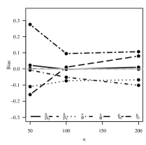
(e) Log-$t$, $q=0.5$

(f) Log-$t$, $q=0.75$

(g) Log-PE, $q=0.25$

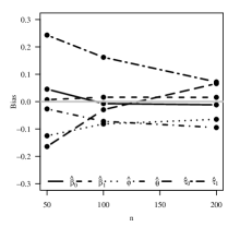
(h) Log-PE, $q=0.5$

(i) Log-PE, $q=0.75$

Figure 1: Biases of the CML estimators for the model QLS-ARMAX(1,1).

(a) Log-HP, $q=0.25$

(b) Log-HP, $q=0.5$

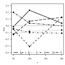
(c) Log-HP, $q=0.75$

(d) Log-CN, $q=0.25$

(e) Log-CN, $q=0.5$

(f) Log-CN, $q=0.75$

(g) Log-SL, $q=0.25$

(h) Log-SL, $q=0.5$

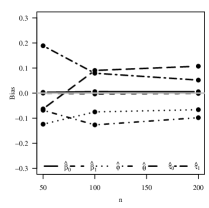
(i) Log-SL, $q=0.75$

Figure 2: Biases of the CML estimators for the model QLS-ARMAX(1,1). (continuation)

(a) Log-SN, $q=0.25$

(b) Log-SN, $q=0.5$

(c) Log-SN, $q=0.75$

(d) Log-ST, $q=0.25$

(e) Log-ST, $q=0.5$

(f) Log-ST, $q=0.75$

Figure 3: Biases of the CML estimators for the model QLS-ARMAX(1,1). (continuation)

(a) Log-NO, $q=0.25$

(b) Log-NO, $q=0.5$

(c) Log-NO, $q=0.75$

(d) Log-$t$, $q=0.25$

(e) Log-$t$, $q=0.5$

(f) Log-$t$, $q=0.75$

(g) Log-PE, $q=0.25$

(h) Log-PE, $q=0.5$

(i) Log-PE, $q=0.75$

Figure 4: MSEs of the CML estimators for the model QLS-ARMAX(1,1).

(a) Log-HP, $q=0.25$

(b) Log-HP, $q=0.5$

(c) Log-HP, $q=0.75$

(d) Log-CN, $q=0.25$

(e) Log-CN, $q=0.5$

(f) Log-CN, $q=0.75$

(g) Log-SL, $q=0.25$

(h) Log-SL, $q=0.5$

(i) Log-SL, $q=0.75$

Figure 5: MSEs of the CML estimators for the model QLS-ARMAX(1,1). (continuation).

(a) Log-SN, $q=0.25$

(b) Log-SN, $q=0.5$

(c) Log-SN, $q=0.75$

(d) Log-ST, $q=0.25$

(e) Log-ST, $q=0.5$

(f) Log-ST, $q=0.75$

Figure 6: MSEs of the CML estimators for the model QLS-ARMAX(1,1). (continuation)

Table 1: Summary statistics for the GCS residuals.

$n$ $q$ Log-NO Log-$t$ Log-PE Log-HP Log-SL Log-SN Log-ST 50 0.25 MN 0.9991 0.9940 0.9959 0.9919 0.9920 0.9994 0.9907 MD 0.6997 0.7027 0.6953 0.6964 0.6934 0.7010 0.6971 SD 0.9833 0.9711 0.9816 0.9719 0.9797 0.9836 0.9708 CS 1.5226 1.4980 1.5362 1.5028 1.5375 1.5245 1.5061 CK 2.4895 2.4122 2.5715 2.4168 2.5973 2.5059 2.4421 0.5 MN 1.0011 0.9977 1.0005 0.9977 0.9969 1.0021 0.9957 MD 0.6949 0.6971 0.6943 0.6975 0.6951 0.6991 0.6950 SD 0.9928 0.9820 0.9871 0.9804 0.9830 0.9896 0.9797 CS 1.5518 1.5264 1.5342 1.5197 1.5303 1.5299 1.5259 CK 2.6126 2.5199 2.5535 2.4871 2.5279 2.4962 2.5220 0.75 MN 1.0003 1.0048 1.0041 1.0067 1.0019 1.0040 1.0030 MD 0.6915 0.6963 0.6921 0.6981 0.6945 0.6959 0.6936 SD 0.9986 0.9948 0.9982 0.9936 0.996 0.9990 0.9931 CS 1.5792 1.5443 1.5688 1.5295 1.5625 1.5689 1.5455 CK 2.7352 2.5677 2.7090 2.5021 2.6630 2.6998 2.5781 100 0.25 MN 0.9984 0.9941 0.9944 0.9964 0.9942 0.9985 0.992 MD 0.6967 0.6915 0.6924 0.6949 0.6956 0.6968 0.6933 SD 0.9882 0.9834 0.9807 0.9793 0.9780 0.9886 0.9748 CS 1.7086 1.6911 1.6640 1.6567 1.6686 1.7115 1.6539 CK 3.6534 3.5562 3.4059 3.3872 3.4256 3.6696 3.3767 0.5 MN 1.0000 0.9977 0.9991 0.9989 0.9973 1.0001 0.9967 MD 0.6950 0.6926 0.6944 0.6947 0.6943 0.6950 0.6941 SD 0.9939 0.9864 0.9847 0.9833 0.9839 0.9944 0.9795 CS 1.7269 1.6915 1.6676 1.662 1.6803 1.7299 1.6560 CK 3.7369 3.5464 3.4263 3.4079 3.4683 3.7543 3.3764 0.75 MN 1.0022 1.0031 1.0054 1.0046 1.0010 1.0023 1.0028 MD 0.6927 0.6946 0.6969 0.6949 0.6930 0.6926 0.6956 SD 1.0023 0.9931 0.9934 0.9942 0.9922 1.0028 0.9877 CS 1.7582 1.6932 1.6813 1.6869 1.6998 1.7623 1.6581 CK 3.9077 3.5347 3.5085 3.5167 3.5665 3.9331 3.3604 200 0.25 MN 0.9977 0.9941 0.9958 0.9961 0.9977 0.9977 0.9940 MD 0.6922 0.6914 0.6917 0.6933 0.6928 0.6922 0.6912 SD 0.9967 0.9813 0.9827 0.9796 0.9889 0.9968 0.9808 CS 1.8667 1.7675 1.7594 1.7430 1.7981 1.8681 1.7703 CK 4.7826 4.1765 4.1439 4.0539 4.3011 4.7930 4.2046 0.5 MN 1.0004 0.9973 0.9993 0.9978 0.9984 1.0004 0.9966 MD 0.6940 0.6939 0.6934 0.6940 0.6937 0.6940 0.6932 SD 1.0000 0.9831 0.9866 0.9840 0.9902 1.0001 0.9828 CS 1.8761 1.7688 1.7675 1.7632 1.8040 1.8775 1.7717 CK 4.8556 4.1837 4.1859 4.1637 4.3490 4.8662 4.2033 0.75 MN 1.0044 1.0015 1.0037 1.0004 1.0029 1.0044 1.0004 MD 0.6956 0.6966 0.6953 0.6941 0.6948 0.6956 0.6956 SD 1.0069 0.9872 0.9927 0.9879 0.9977 1.0070 0.9868 CS 1.8957 1.7634 1.7758 1.7687 1.8163 1.8974 1.7682 CK 4.9945 4.1421 4.2354 4.1946 4.3895 5.0080 4.1700

Table 2: Summary statistics for the RQ residuals.

$n$ $q$ Log-NO Log-$t$ Log-PE Log-HP Log-SL Log-SN Log-ST 50 0.25 MN -0.0011 -0.0009 -0.0043 -0.0065 -0.0071 -0.0008 -0.0058 MD 0.0030 0.0084 0.0015 0.0013 -0.0039 0.0046 0.0017 SD 1.0100 0.9995 1.0088 1.0059 1.0066 1.0100 1.0020 CS -0.0163 -0.0174 -0.0196 -0.0283 -0.0121 -0.0155 -0.0198 CK -0.3184 -0.3671 -0.3095 -0.3476 -0.3257 -0.3218 -0.3593 0.5 MN 0.0000 0.0012 0.0005 -0.0004 -0.0004 0.0015 -0.0009 MD -0.0032 0.0016 -0.0003 0.0021 -0.0021 0.0017 -0.0014 SD 1.0096 1.0017 1.0076 1.0044 1.0028 1.0095 1.0012 CS 0.0161 0.0004 -0.0009 -0.0042 0.0052 0.0043 0.0007 CK -0.3373 -0.3482 -0.3378 -0.3632 -0.3446 -0.3363 -0.3538 0.75 MN -0.0013 0.0069 0.0034 0.0073 0.0033 0.0022 0.0055 MD -0.0074 0.0007 -0.0028 0.0033 -0.0026 -0.0019 -0.0027 SD 1.0091 1.0040 1.0081 1.0070 1.005 1.0104 1.0028 CS 0.0342 0.0182 0.0224 0.0097 0.0245 0.0247 0.0218 CK -0.3136 -0.3383 -0.3182 -0.3546 -0.3205 -0.3226 -0.3414 100 0.25 MN -0.0019 -0.0045 -0.0059 -0.0015 -0.0033 -0.0018 -0.005 MD 0.0020 -0.0036 -0.0017 0.0008 0.0009 0.0020 -0.0015 SD 1.0054 1.0007 1.0040 1.0002 1.0003 1.0056 0.9980 CS -0.0153 -0.0045 -0.0134 -0.0085 -0.0188 -0.0155 -0.0098 CK -0.1722 -0.2129 -0.2390 -0.2513 -0.2184 -0.1679 -0.2549 0.5 MN -0.0005 0.0002 -0.0002 0.0010 -0.0002 -0.0005 0.0007 MD -0.0003 -0.0024 0.0007 0.0004 -0.0011 -0.0003 -0.0006 SD 1.0047 0.9991 1.0025 0.9999 0.9993 1.0049 0.9966 CS 0.0052 0.0026 -0.0046 0.002 -0.0010 0.0051 -0.0001 CK -0.1824 -0.2120 -0.2427 -0.2582 -0.2222 -0.1787 -0.2546 0.75 MN 0.0010 0.0051 0.0054 0.0057 0.0026 0.0009 0.0060 MD -0.0031 0.0002 0.0039 0.0007 -0.0023 -0.0032 0.0014 SD 1.0051 1.0005 1.0042 1.0015 1.0008 1.0053 0.9982 CS 0.0250 0.0089 0.0038 0.0186 0.0111 0.0250 0.0103 CK -0.1727 -0.2118 -0.2367 -0.2483 -0.2113 -0.1685 -0.2566 200 0.25 MN -0.0033 -0.0035 -0.0039 -0.0017 -0.0007 -0.0033 -0.0035 MD -0.0024 -0.0030 -0.0022 -0.0004 -0.0014 -0.0024 -0.0032 SD 1.0035 0.9969 1.0009 0.9977 0.9990 1.0035 0.9969 CS -0.0027 -0.0010 -0.0089 -0.0046 -0.0002 -0.0027 -0.0028 CK -0.0649 -0.1794 -0.1853 -0.2119 -0.1369 -0.0632 -0.1787 0.5 MN 0.0001 0.0007 0.0002 -0.0003 0.0001 0.0001 -0.0002 MD -0.0003 0.0001 -0.0002 0.0003 -0.0003 -0.0003 -0.0008 SD 1.0024 0.9958 1.0000 0.9982 0.9989 1.0024 0.9959 CS 0.0066 0.0002 -0.0011 -0.0003 0.0021 0.0066 0.0001 CK -0.0697 -0.1746 -0.1830 -0.1899 -0.1331 -0.0683 -0.1740 0.75 MN 0.0035 0.0044 0.0040 0.0021 0.0038 0.0035 0.0033 MD 0.0020 0.0035 0.0023 0.0006 0.0010 0.0020 0.0022 SD 1.0036 0.9971 1.0010 0.9985 1.0003 1.0036 0.9969 CS 0.0155 0.0019 0.0067 0.0075 0.0116 0.0155 0.0028 CK -0.0639 -0.1804 -0.1835 -0.1943 -0.1265 -0.0622 -0.1767

4 Application to Walmart sales data

To illustrate the applicability of the proposed models, we considered the dataset on the competition "M5 Forecasting - Accuracy" (Makridakis et al.,, 2021). This dataset corresponds to the daily sales ($Y_{t}$) history of 30,491 Walmart products and is related to 10 stores of the hypermarket chain in three different US states. For the purpose of analysis, the sets of all these time series were grouped to form only one time series composed of the total daily sales. Then, the series was adjusted for trend and multiple seasonality using the MSTL decomposition (Hyndman and Athanasopoulos,, 2018; Bandara et al.,, 2021), and considering three types of seasonality that are typical of daily sales series: annual (cycle of 365.25 observations), monthly (cycle of 30.43 observations) and weekly (cycle of 7 observations). We thus obtained a stationary series resulting from the filtering of the trend and multiple seasonalities; see Figure 7 for a plot of this series. The explanatory variables are $snapca_{1t}$, snapTX ($snaptx_{2t}$), Mother’s Day ($mother_{3t}$) and Thanksgiving ($thanks_{4t}$). The dataset prepared for this study is available upon request.

Figure 7: Daily sales of 30,491 Walmart products.

Initially, we can fit a linear regression model and analyze the autocorrelation function (ACF) and partial autocorrelation function (PACF). Considering the daily sales ($Y_{t}$) as the response variable, we can assume the following structure:

$$Y_{t}=\beta_{0}+\beta_{1}snapca_{1t}+\beta_{2}snaptx_{2t}+\beta_{3}mother_{3t}+\beta_{4}thanks_{4t}+\varepsilon_{t},$$ (12)

where $\varepsilon_{t}$ is a random error consisting of independent random variables which are identically distributed as normal with zero mean and variance $\sigma_{\varepsilon}^{2}$. Figure 8 shows the ACF and PACF of the residuals from the least squares fit of (12). From this figure, we observe that the residuals are autocorrelated and ARMA models seem to be more appropriate for these data.

Figure 8: Plots of ACF (left) and PACF (right) of the residuals from the fitted regression model with the Walmart sales data.

In addition to the limitation due to autocorrelated residuals, other important aspects that must be observed are the characteristics in the data. Table 3 reports descriptive statistics of the observed Walmart sales, including the mean, median, standard deviation (SD), coefficient of variation (CV), skewness (CS), (excess) kurtosis (CK), and minimum and maximum values. From this table, we observe skewness and high kurtosis in the data. Such observations make the proposed log-symmetric quantile ARMA models good candidates for fitting the data since they account for asymmetry with or without heavy tails.

Table 3: Summary statistics for the Walmart sales data.

Mean	Median	SD	CV	CS	CK	minimum	maximum	size
34488.87	34460.03	1878.172	5.446%	0.165	10.396	17256.78	53304.64	330

We then analyze the Walmart sales data using the QLS-ARMAX($p,q$) models, expressed as

$$\eta_{t}=\log(Q_{t}) = \beta_{0}+\beta_{1}snapca_{1t}+\beta_{2}snaptx_{2t}+\beta_{3}mother_{3t}+\beta_{4}thanks_{4t}$$

$$+\sum_{i=1}^{p}\phi_{i}\left[h(Y_{t-i})-(\beta_{0}+\beta_{1}snapca_{1{t-i}}+\beta_{2}snaptx_{2{t-i}}+\beta_{3}mother_{3{t-i}}\right.$$

$$\left.+\beta_{4}thanks_{4{t-i}})\right]+\sum_{j=1}^{q}\theta_{j}r_{t-j},\quad t=\max\{p,q\},\ldots,n,$$

$$\gamma_{t}=\log(\kappa_{t}) = \tau_{0}+\tau_{1}mother_{1t}+\tau_{2}thanks_{2t},\quad t=\max\{p,q\},\ldots,n.$$

First, we have to find the best model among the class of QLS-ARMAX($p,q$) models that include the log-normal (log-NO), log-Student-$t$ (log-$t$), log-power-exponential (log-PE), log-hyperbolic (log-HP), log-slash (log-SL), log-contaminated-normal (log-CN), extended Birnbaum-Saunders (EBS) and extended Birnbaum-Saunders-$t$ (EBS-$t$) distributions. To this end, we fit the models based on a grid of values of $q\in\{0.01,0.02,\dots,0.99\}$. Then, we compute the averages of the corresponding vAkaike (AIC), Bayesian (BIC), corrected Akaike (CAIC) and Hannan-Quinn (HQIC) information criteria values. From Table 4, we observe that the log-$t$ quantile ARMA model provides the best adjustment compared to the other log-symmetric quantile ARMA models based on the values of AIC, BIC, CAIC and HIC.

Table 4: Averages of the AIC, BIC, CAIC and HQIC values computed across $q\in\{0.01,0.02,\ldots,0.98,0.99\}$ for the indicated QLS-ARMAX models with the Walmart sales data.

Indicator	log-NO	log-$t$	log-PE	log-HP	log-SL	log-CN	EBS	EBS-$t$
AIC	-6219.350	-6705.274	-6643.247	-6647.953	-6682.070	-6604.540	-6190.254	-6704.203
BIC	-6130.214	-6616.138	-6554.112	-6558.818	-6592.935	-6515.405	-6095.547	-6615.068
CAIC	-6219.137	-6705.062	-6643.035	-6647.741	-6681.858	-6604.328	-6190.010	-6703.991
HQIC	-6218.960	-6704.885	-6642.858	-6647.564	-6681.681	-6604.151	-6189.840	-6703.814

In Figure 9, we plot the estimated parameters of the log-$t$ quantile ARMA model across $q\in\{0.01,\ldots,0.99\}$. We notice the coefficients $\hat{\beta}_{0},\hat{\beta}_{1},\hat{\beta}_{2}$ to increase with an increase in the quantile value. Futhermore, we also note that the other coefficients do not vary according to the quantile fixed in the fitted model.

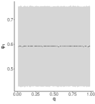
(a) $\phi_{1}$

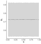
(b) $\theta_{1}$

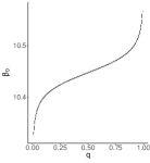
(c) $\beta_{0}$

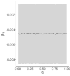
(d) $\beta_{1}$

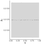
(e) $\beta_{2}$

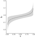
(f) $\beta_{3}$

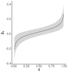
(g) $\beta_{4}$

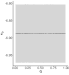
(h) $\tau_{0}$

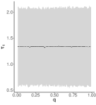
(i) $\tau_{1}$

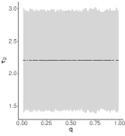
(j) $\tau_{2}$

Figure 9: Estimated parameters in the log-$t$ quantile ARMA model across $q$ for the Walmart sales data.

In Figure 10, we present the QQ plots with simulated, ACF and PACF of the Cox-Snell residuals (CS) and randomized quantile residuals (RQ) corresponding to the proposed model and considering the indicated quantile as $q=0.5$. From Figure 10, we note that the CS and RQ residuals indicate that the postulated model presents a good fit to the Walmart sales data. The ACF and PACF plots of the CS and RQ residuals indicate that the log-$t$-ARMA(1,1) quantile model produces non-autocorrelated residuals.

To assess the quality of the forecasts provided by the fitted log-$t$-ARMA quantile model, we divided the Walmart sales data as follows: the first 1,900 observations were used to fit the model, whereas the last 41 observations were used in assessing the quality of forecasts. For comparison purposes, we also considered the fit of the ARMAX(1,1) model to the Walmart sales data.

In Table 5, we present the ML estimates of the parameters of the log-$t$-ARMA(1,1) quantile model with $q=0.5$ and the ARMAX(1,1) model. In Table 6, we present some error measures of the point and interval forecasts. For the point error measures, we consider the following: root of mean squared error (RMSE), mean absolute error (MAE), mean absolute scaled error (MASE) and symmetric mean absolute percentage error (SMAPE). For the interval error measure, we only consider the mean scaled interval score (MSIS); see Makridakis et al., (2021) for more details about these measures. In particular, for the MSIS metric, we are interested in comparing the 95% interval obtained with the estimates of the log-$t$-ARMA model fitted for the quantiles $q=0.025,0.975$ and the asymptotic prediction interval of 95% based on the ARMAX model. The RMSE and MSIS metrics are smaller for the log-$t$ quantile model, indicating that the quantile model is better according to the metrics. On the other hand, for the MAE and MASE metrics, the results are smaller for the ARMAX model, indicates that it presents predictions according to these best metrics. Finally, regarding sMAPE, the value is the same for both models.

Table 5: ML estimates and standard errors in parentheses for the log-$t$ ARMA with $q=0.5$ and $\hat{\vartheta}=4$, and ARMAX model for the first 1,900 observations of the Walmart sales data.

Estimate (standard error) Model Parameter Intercept snapca snapt mother thanks log-$t$ $\hat{\beta}$ 10.4448(0.0012) -0.0052(0.0021) 0.0143(0.0021) -0.0268(0.0165) 0.0227(0.0281) $\hat{\tau}$ -6.8343(0.0436) 1.2365(0.4200) 2.2772(0.3859) $\hat{\phi}$ 0.9191(0.0459) $\hat{\theta}$ -0.6618(0.0510) ARMAX $\hat{\beta}$ 34390.22(193.54) -151.39(94.71) 543.87(90.9) -1251.99(412.52) 1227.12(413.52) $\hat{\phi}$ 0.9767(0.0077) $\hat{\theta}$ -0.8869(0.0152)

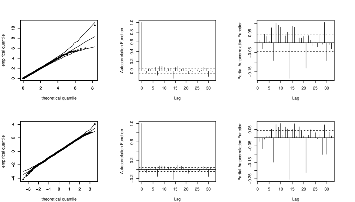
Figure 10: QQ plot with simulated envelopes (left), ACF (center) and PACF plots (right) of the CS and RQ residuals corresponding to the log-$t$ ARMA model with $q=0.5$ and $\hat{\vartheta}=4$ based on the Walmart sales data.

In Figure 11, we present the forecasts for the last 41 observations of the Walmart sales data based on the log-$t$-ARMA and ARMAX models. We can see from the Figure 11 that the prediction intervals contain most of the real values. In addition, we can notice that closer to the prediction horizon, the predicted values for the log-$t$-ARMA quantile and ARMAX models are less accurate.

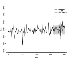
(a) log-$t$-ARMA(1,1)

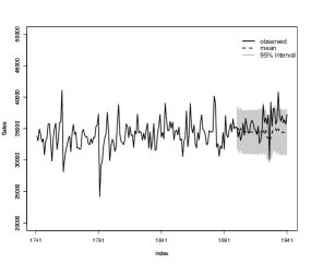
(b) ARMAX(1,1)

Figure 11: 95% interval prediction for the last 41 observations of the Walmart sales data by the log-$t$-ARMA(1,1) quantile model (left) and the ARMAX(1,1) model (right).

Table 6: Error metrics in the log-$t$-ARMA(1,1) quantile model and the ARMAX(1,1) model based on the last 41 observations of the Walmart sales data.

Model	RMSE	MAE	MASE	SMAPE	MSIS
log-$t$	2193.11	1796.17	1.17	102.44	174.26
ARMAX	2210.80	1760.71	1.15	102.44	183.63

5 Concluding remarks

In this paper, we have proposed parametric quantile autoregressive moving average models based on a reparameterized version of the log-symmetric distributions, which is indexed by a quantile parameter. Thus, the proposed autoregressive moving average models is defined in terms of a conditional quantile, allowing different estimates for different quantiles of interest. The proposed model accommodates covariates and can be seen as an extension to the case where there is temporal dependence of the log-symmetric quantile regression models. A Monte Carlo simulation was carried out to evaluate the performance of the proposed models and the estimation method. We have applied the proposed models and some other existing autoregressive moving average models to a real data set correponding to daily sales of 30,491 Walmart products. The results support the suitability of the proposed log-symmetric quantile autoregressive moving average models, both in terms of model fitting and forecasting ability.

Appendix A Stationarity conditions

Proof A.1

Let $\bm{\Phi}(B)=\sum_{i=0}^{q}\phi_{i}B^{i}$ and $\bm{\Theta}(B)=\sum_{i=0}^{q}\theta_{i}B^{i}$ be the moving average polynomial and the autoregressive polynomial, with $\theta_{0}=\phi_{0}=1$ e $y_{t}B^{i}=y_{t-i}$, respectively. The lag operator being $\bm{\Psi}(B)=\bm{\Theta}(B)\bm{\Phi}(B)^{-1}=\sum_{i=0}^{\infty}\psi_{i}B^{i}$ with $\psi_{0}=1$ e $\bm{\Phi}(B)$ invertible, the QLS-ARMAX($p,q$) model can be rewritten as

$$\bm{\Phi}(B)(Y_{t}-h^{-1}(\bm{x_{t}^{\top}\beta}{\color[rgb]{0,0,0}+\varrho_{t}})) = \bm{\Theta}(B){\color[rgb]{0,0,0}\varepsilon}_{t},$$

$$Y_{t} = h^{-1}(\bm{x_{t}^{\top}\beta}{\color[rgb]{0,0,0}+\varrho_{t}})+\bm{\Psi}(B){\color[rgb]{0,0,0}\varepsilon}_{t}.$$

Thus, the marginal expectation of $Y_{t}$ in the QLS-ARMAX($p,q$) model is given by

$$\mathrm{E}[Y_{t}] = \mathrm{E}[h^{-1}(\bm{x_{t}^{\top}\beta}{\color[rgb]{0,0,0}+\varrho_{t}})+\bm{\Psi}(B){\color[rgb]{0,0,0}\varepsilon}_{t}],$$

$$= {\color[rgb]{0,0,0}\mathrm{E}}[h^{-1}(\bm{x_{t}^{\top}\beta}{\color[rgb]{0,0,0}+\varrho_{t}})]+\bm{\Psi}(B)\mathrm{E}[{\color[rgb]{0,0,0}\varepsilon}_{t}],$$

$$= {\color[rgb]{0,0,0}\mathrm{E}}[h^{-1}(\bm{x_{t}^{\top}\beta}{\color[rgb]{0,0,0}+\varrho_{t}})],$$

where the error ${\color[rgb]{0,0,0}\varepsilon_{t}=Y_{t}-Q_{t}}$, with ${\color[rgb]{0,0,0}\ Q_{t}=h^{-1}(\bm{x_{t}^{\top}\beta}{\color[rgb]{0,0,0}+\varrho_{t}})}$, is an MDS sequence with $\mathrm{E}[{\color[rgb]{0,0,0}\varepsilon}_{t}]=0$ for all $t$.

Proof A.2

Rewriting $Y_{t}=Q_{t}+r_{t}$, where $\mathrm{E}[r_{t}]=0$ and $\mathrm{Cov}[r_{t},r_{s}]=0$, we have

$$\mathrm{Var}[r_{t}] = \mathrm{E}[\mathrm{Var}[r_{t}|\mathcal{B}_{t-1}]]+\mathrm{Var}[\mathrm{E}[r_{t}|\mathcal{B}_{t-1}]]=\mathrm{E}[\mathrm{Var}[r_{t}|\mathcal{B}_{t-1}]]$$ (13)

$$= \mathrm{E}[\mathrm{Var}[Y_{t}-Q_{t}|\mathcal{B}_{t-1}]]=\mathrm{E}[\mathrm{Var}[Y_{t}|\mathcal{B}_{t-1}]].$$

Then, by (13), the variance of $Y_{t}$ is given by

$$\mathrm{Var}[Y_{t}] = \mathrm{Var}[h^{-1}(\bm{x_{t}^{\top}\beta})+\bm{\Psi}(B)r_{t}]=\mathrm{Var}[\bm{\Psi}(B)r_{t}]=\mathrm{Var}\left[\sum_{i=0}^{\infty}\psi_{i}r_{t-i}\right]$$ (14)

$$= \sum_{i=0}^{\infty}\psi_{i}^{2}\mathrm{Var}\left[r_{t-i}\right]=\sum_{i=0}^{\infty}\psi_{i}^{2}\mathrm{E}[\mathrm{Var}[Y_{t-i}|\mathcal{B}_{t-i-1}]].$$

Proof A.3

From Theorems 2.1 and 2.2, we have

$$\mathrm{Cov}[Y_{t},Y_{t-k}] = \mathrm{Cov}\left[h^{-1}(\bm{x_{t}^{\top}\beta})+\sum_{i=0}^{\infty}\psi_{i}r_{t-i},h^{-1}(\bm{x_{t-k}^{\top}\beta})+\sum_{i=0}^{\infty}\psi_{i+k}r_{t-k-i}\right]$$ (15)

$$= \sum_{i=0}^{\infty}\psi_{i}\psi_{i+k}\mathrm{Cov}\left[r_{t-i},r_{t-k-i}\right]=\sum_{i=0}^{\infty}\psi_{i}\psi_{i+k}\mathrm{Var}\left[r_{t-i}\right]$$

$$= \sum_{i=0}^{\infty}\psi_{i}\psi_{i+k}\mathrm{E}[\mathrm{Var}[Y_{t-i}|\mathcal{B}_{t-i-1}]].$$

Then, by (13) and (15), we have

$$\mathrm{Corr}[Y_{t},Y_{t-k}] = \frac{\mathrm{Cov}[Y_{t},Y_{t-k}]}{\sqrt{\mathrm{Var}[Y_{t}]\mathrm{Var}[Y_{t-k}]}}$$

$$= \frac{\sum_{i=0}^{\infty}\psi_{i}\psi_{i+k}\mathrm{E}[\mathrm{Var}[Y_{t-i}|\mathcal{B}_{t-i-1}]]}{\sqrt{\sum_{i=0}^{\infty}\psi_{i}^{2}\mathrm{E}[\mathrm{Var}[Y_{t-i}|\mathcal{B}_{t-i-1}]]}\sqrt{\sum_{i=0}^{\infty}\psi_{i+k}^{2}\mathrm{E}[\mathrm{Var}[Y_{t-k-i}|\mathcal{B}_{t-k-i-1}]]}}$$

$$= \frac{\sum_{i=0}^{\infty}\psi_{i}\psi_{i+k}\mathrm{E}[\mathrm{Var}[Y_{t-i}|\mathcal{B}_{t-i-1}]]}{\prod_{j\in\left\{0,k\right\}}\sqrt{\sum_{i=0}^{\infty}\psi_{i+j}^{2}\mathrm{E}[\mathrm{Var}[Y_{t-j-i}|\mathcal{B}_{t-j-i-1}]]}}.$$

Appendix B Hessian matrix

We denoted the Hessian matrix by ${\cal J}(\bm{\zeta})$, which is given by

$${\cal J}(\bm{\zeta})=\begin{bmatrix}{\cal J}_{\bm{\beta\beta}}(\bm{\zeta})&{\cal J}_{\bm{\beta\tau}}(\bm{\zeta})&{\cal J}_{\bm{\beta\phi}}(\bm{\zeta})&{\cal J}_{\bm{\beta\theta}}(\bm{\zeta})\\ {\cal J}_{\bm{\tau\beta}}(\bm{\zeta})&{\cal J}_{\bm{\tau\tau}}(\bm{\zeta})&{\cal J}_{\bm{\tau\phi}}(\bm{\zeta})&{\cal J}_{\bm{\tau\theta}}(\bm{\zeta})\\ {\cal J}_{\bm{\phi\beta}}(\bm{\zeta})&{\cal J}_{\bm{\phi\tau}}(\bm{\zeta})&{\cal J}_{\bm{\phi\phi}}(\bm{\zeta})&{\cal J}_{\bm{\phi\theta}}(\bm{\zeta})\\ {\cal J}_{\bm{\theta\beta}}(\bm{\zeta})&{\cal J}_{\bm{\theta\tau}}(\bm{\zeta})&{\cal J}_{\bm{\theta\phi}}(\bm{\zeta})&{\cal J}_{\bm{\theta\theta}}(\bm{\zeta})\end{bmatrix}$$

so that we get the second derivative of $\ell(\bm{\zeta})_{m,n}$ with respect to $\bm{\zeta}=(\bm{\beta,\tau,\phi,\theta})^{\top}$. For the main diagonal elements of Hessian matrix, first, we have $\beta_{s}$, $s=0,\ldots,k$,

$${\cal J}_{\bm{\beta\beta}}(\bm{\zeta}) = \frac{\partial^{2}}{\partial\beta_{s}^{2}}\ell(\bm{\zeta})_{m,n},\quad s=0,1\ldots,k$$

$$= \sum_{t=m+1}^{n}\frac{1}{\sqrt{\kappa_{t}}}\left\{\frac{\partial^{2}Q_{t}}{\partial\eta_{t}^{2}}\frac{\partial\eta_{t}}{\partial\beta_{s}}\left[v(z_{t})\frac{z_{t}}{Q_{t}}\frac{\partial\eta_{t}}{\partial\beta_{s}}\right]+\frac{\partial Q_{t}}{\partial\eta_{t}}\left(\frac{\partial}{\partial\beta_{s}}\left[v(z_{t})\frac{z_{t}}{Q_{t}}\frac{\partial\eta_{t}}{\partial\beta_{s}}\right]\right)\right\}$$

$$= \sum_{t=m+1}^{n}\frac{1}{\sqrt{\kappa_{t}}}\left\{v(z_{t})\frac{z_{t}}{Q_{t}}\frac{\partial^{2}Q_{t}}{\partial\eta_{t}^{2}}\left(\frac{\partial\eta_{t}}{\partial\beta_{s}}\right)^{2}+\frac{\partial Q_{t}}{\partial\eta_{t}}\left[\frac{\partial v(z_{t})}{\partial\beta_{s}}\left(\frac{z_{t}}{Q_{t}}\frac{\partial\eta_{t}}{\partial\beta_{s}}\right)+v(z_{t})\frac{\partial}{\partial\beta_{s}}\left(\frac{z_{t}}{Q_{t}}\frac{\partial\eta_{t}}{\partial\beta_{s}}\right)\right]\right\}$$

$$= \sum_{t=m+1}^{n}\frac{1}{\sqrt{\kappa_{t}}}\left\{v(z_{t})\frac{z_{t}}{Q_{t}}\frac{\partial^{2}Q_{t}}{\partial\eta_{t}^{2}}\left(\frac{\partial\eta_{t}}{\partial\beta_{s}}\right)^{2}+\frac{\partial Q_{t}}{\partial\eta_{t}}\left[\frac{\partial v(z_{t})}{\partial\beta_{s}}\left(\frac{z_{t}}{Q_{t}}\frac{\partial\eta_{t}}{\partial\beta_{s}}\right)+v(z_{t})\left[\left(\frac{\partial z_{t}}{\partial\beta_{s}}\frac{1}{Q_{t}}\frac{\partial\eta_{t}}{\partial\beta_{s}}\right)+\right.\right.\right.$$

$$\left.\left.\left.z_{t}\frac{\partial}{\partial\beta_{s}}\left(\frac{1}{Q_{t}}\frac{\partial\eta_{t}}{\partial\beta_{s}}\right)\right]\right]\right\}$$

where $v^{\prime}(u)=-2[g^{\prime\prime}(u)g(u)-g^{\prime}(u)^{2}]/g(u)^{2},$ $g^{\prime\prime}(u)=\text{d}^{2}g(u)/\text{d}u^{2}$, with the partial derivatives

$$\frac{\partial v(z_{t})}{\partial\beta_{s}}=-2\frac{v^{\prime}(z_{t})}{\sqrt{\kappa_{t}}}\frac{z_{t}}{Q_{t}}\frac{\partial Q_{t}}{\partial\eta_{t}}\frac{\partial\eta_{t}}{\partial\beta_{s}},\qquad\frac{\partial z_{t}}{\partial\beta_{s}}=-\frac{1}{\sqrt{\kappa_{t}}}\frac{1}{Q_{t}}\frac{\partial Q_{t}}{\partial\eta_{t}}\frac{\partial\eta_{t}}{\partial\beta_{s}}$$

and the partial derivatives are given by

$$\frac{\partial}{\partial\beta_{s}}\left(\frac{1}{Q_{t}}\frac{\partial\eta_{t}}{\partial\beta_{s}}\right)=-\frac{1}{Q_{t}^{2}}\frac{\partial Q_{t}}{\partial\eta_{t}}\left(\frac{\partial\eta_{t}}{\partial\beta_{s}}\right)^{2}-\frac{1}{Q_{t}}\frac{\partial^{2}\eta_{t}}{\partial\beta_{s}^{2}},\qquad\frac{\partial\eta_{t}}{\partial\beta_{s}}=x_{t,s}-\left(\sum_{i=1}^{p}\phi_{i}x_{t-i,s}+\sum_{j=1}^{q}\theta_{j}\frac{\partial Q_{t-j}}{\partial\eta_{t-j}}\frac{\partial\eta_{t-j}}{\partial\beta_{s}}\right),$$

$$\frac{\partial^{2}\eta_{t}}{\partial\beta_{s}^{2}}=-\sum_{j=1}^{q}\theta_{j}\left(\frac{\partial^{2}Q_{t-j}}{\partial\eta_{t-j}^{2}}\left(\frac{\partial\eta_{t-j}}{\partial\beta_{s}}\right)^{2}+\frac{\partial Q_{t-j}}{\partial\eta_{t-j}}\frac{\partial^{2}\eta_{t-j}}{\partial\beta_{s}^{2}}\right).$$

For $\tau_{s}$, $s=0,\ldots,l$, we have

$${\cal J}_{\bm{\tau\tau}}(\bm{\zeta}) = \frac{\partial^{2}}{\partial\tau_{s}^{2}}\ell(\bm{\zeta})_{m,n},\quad s=0,1\ldots,l$$

$$= \frac{1}{2}\sum_{t=m+1}^{n}w_{t,s}\left\{\frac{\partial}{\partial\tau_{s}}\left(\frac{1}{\kappa_{t}}\frac{\partial\kappa_{t}}{\partial\gamma_{t}}\right)[v(z_{t})z_{t}(z_{t}-z_{p})-1]+\left(\frac{1}{\kappa_{t}}\frac{\partial\kappa_{t}}{\partial\gamma_{t}}\right)\frac{\partial}{\partial\tau_{s}}[v(z_{t})z_{t}(z_{t}-z_{p})-1]\right\},$$

where, the partial derivatives which given by

$$\frac{\partial}{\partial\tau_{s}}\left(\frac{1}{\kappa_{t}}\frac{\partial\kappa_{t}}{\partial\gamma_{t}}\right)=-\frac{1}{\kappa_{t}^{2}}\left(\frac{\partial\kappa_{t}}{\partial\gamma_{t}}\right)^{2}w_{t,s}+\frac{1}{\kappa_{t}}\frac{\partial^{2}\kappa_{t}}{\partial\gamma_{t}^{2}}w_{t,s}=\frac{1}{\kappa_{t}}w_{t,s}\left[\frac{\partial^{2}\kappa_{t}}{\partial\gamma_{t}^{2}}-\frac{1}{\kappa_{t}}\left(\frac{\partial\kappa_{t}}{\partial\gamma_{t}}\right)^{2}\right],$$

with

$$\frac{\partial}{\partial\tau_{s}}[v(z_{t})z_{t}(z_{t}-z_{p})-1] = \frac{\partial v(z_{t})}{\partial\tau_{s}}[z_{t}(z_{t}-z_{p})-1]+v(z_{t})\frac{\partial}{\partial\tau_{s}}\left[z_{t}(z_{t}-z_{p})-1\right]$$

$$= -\frac{v^{\prime}(z_{t})}{\kappa_{t}}z_{t}(z_{t}-z_{p})\frac{\partial\kappa_{t}}{\partial\gamma_{t}}w_{t,s}[z_{t}(z_{t}-z_{p})-1]+v(z_{t})$$

$$\left[\frac{\partial z_{t}}{\partial\tau_{s}}(z_{t}-z_{p})+z_{t}\frac{\partial}{\partial\tau_{s}}(z_{t}-z_{p})\right]$$

$$= -\frac{v^{\prime}(z_{t})}{\kappa_{t}}z_{t}(z_{t}-z_{p})[z_{t}(z_{t}-z_{p})-1]\frac{\partial\kappa_{t}}{\partial\gamma_{t}}w_{t,s}+v(z_{t})$$

$$\left[-\frac{1}{2}\frac{1}{\kappa_{t}}(z_{t}-z_{p})^{2}\frac{\partial\kappa_{t}}{\partial\gamma_{t}}w_{t,s}-\frac{1}{2}\frac{z_{t}}{\kappa_{t}}(z_{t}-z_{p})\frac{\partial\kappa_{t}}{\partial\gamma_{t}}w_{t,s}\right]$$

$$= -\frac{v^{\prime}(z_{t})}{\kappa_{t}}z_{t}(z_{t}-z_{p})[z_{t}(z_{t}-z_{p})-1]\frac{\partial\kappa_{t}}{\partial\gamma_{t}}w_{t,s}-\frac{1}{2}\frac{v(z_{t})}{\kappa_{t}}(z_{t}-z_{p})\frac{\partial\kappa_{t}}{\partial\gamma_{t}}w_{t,s}$$

$$[(z_{t}-z_{p})+z_{t}].$$

For $\phi_{s}$, $s=0,\ldots,p$, we have the partial derivatives

$${\cal J}_{\bm{\phi\phi}}(\bm{\zeta}) = \frac{\partial^{2}}{\partial\phi_{s}^{2}}\ell_{m,n}({\bm{\zeta}}),\quad s=1,\ldots,p$$

$$= \sum_{t=m+1}^{n}\frac{1}{\sqrt{\kappa_{t}}}\left\{\frac{\partial v(z_{t})}{\partial\phi_{s}}\left[\frac{z_{t}}{Q_{t}}\frac{\partial Q_{t}}{\partial\eta_{t}}\frac{\partial\eta_{t}}{\partial\phi_{s}}\right]+v(z_{t})\left[\frac{\partial}{\partial\phi_{s}}\left(\frac{z_{t}}{Q_{t}}\frac{\partial Q_{t}}{\partial\eta_{t}}\frac{\partial\eta_{t}}{\partial\phi_{s}}\right)\right]\right\}$$

$$= \sum_{t=m+1}^{n}\frac{1}{\sqrt{\kappa_{t}}}\left\{-2\frac{v^{\prime}(z_{t})}{\sqrt{\kappa_{t}}}\frac{z_{t}}{Q_{t}}\frac{\partial Q_{t}}{\partial\eta_{t}}\frac{\partial\eta_{t}}{\partial\phi_{s}}\left[\frac{z_{t}}{Q_{t}}\frac{\partial Q_{t}}{\partial\eta_{t}}\frac{\partial\eta_{t}}{\partial\phi_{s}}\right]+v(z_{t})\left[\frac{\partial}{\partial\phi_{s}}\left(\frac{z_{t}}{Q_{t}}\frac{\partial Q_{t}}{\partial\eta_{t}}\frac{\partial\eta_{t}}{\partial\phi_{s}}\right)\right]\right\},$$

where, the partial derivatives which given by

$$\frac{\partial}{\partial\phi_{s}}\left(\frac{z_{t}}{Q_{t}}\frac{\partial Q_{t}}{\partial\eta_{t}}\frac{\partial\eta_{t}}{\partial\phi_{s}}\right) = \frac{\partial z_{t}}{\partial\phi_{s}}\left(\frac{1}{Q_{t}}\frac{\partial Q_{t}}{\partial\eta_{t}}\frac{\partial\eta_{t}}{\partial\phi_{s}}\right)+z_{t}\left[\frac{\partial}{\partial\phi_{s}}\left(\frac{1}{Q_{t}}\frac{\partial Q_{t}}{\partial\eta_{t}}\frac{\partial\eta_{t}}{\partial\phi_{s}}\right)\right]$$

$$= \frac{\partial z_{t}}{\partial\phi_{s}}\left(\frac{1}{Q_{t}}\frac{\partial Q_{t}}{\partial\eta_{t}}\frac{\partial\eta_{t}}{\partial\phi_{s}}\right)+z_{t}\left[\frac{\partial Q_{t}^{-1}}{\partial\phi_{s}}\left(\frac{\partial Q_{t}}{\partial\eta_{t}}\frac{\partial\eta_{t}}{\partial\phi_{s}}\right)+\frac{1}{Q_{t}}\frac{\partial}{\partial\phi_{s}}\left(\frac{\partial Q_{t}}{\partial\eta_{t}}\frac{\partial\eta_{t}}{\partial\phi_{s}}\right)\right]$$

$$= \frac{\partial z_{t}}{\partial\phi_{s}}\left(\frac{1}{Q_{t}}\frac{\partial Q_{t}}{\partial\eta_{t}}\frac{\partial\eta_{t}}{\partial\phi_{s}}\right)+z_{t}\left[\frac{\partial Q_{t}^{-1}}{\partial\phi_{s}}\left(\frac{\partial Q_{t}}{\partial\eta_{t}}\frac{\partial\eta_{t}}{\partial\phi_{s}}\right)+\frac{1}{Q_{t}}\left\{\frac{\partial^{2}Q_{t}}{\partial\eta_{t}^{2}}\left(\frac{\partial\eta_{t}}{\partial\phi_{s}}\right)^{2}+\right.\right.$$

$$\left.\left.\frac{\partial Q_{t}}{\partial\eta_{t}}\frac{\partial^{2}\eta_{t}}{\partial\phi_{s}^{2}}\right\}\right]$$

with the partial derivatives are given by

$$\frac{\partial z_{t}}{\partial\phi_{s}}=-\frac{1}{\sqrt{\kappa_{t}}}\frac{1}{Q_{t}}\frac{\partial Q_{t}}{\partial\eta_{t}}\frac{\partial\eta_{t}}{\partial\phi_{s}},\qquad\frac{\partial Q_{t}^{-1}}{\partial\phi_{s}}=-\frac{1}{Q_{t}^{2}}\frac{\partial Q_{t}}{\partial\eta_{t}}\frac{\partial\eta_{t}}{\partial\phi_{s}}$$

and

$$\frac{\partial\eta_{t}}{\partial\phi_{s}}=\left[h(y_{t-s})-\bm{x_{t-s}^{\top}\beta}\right]-\sum_{j=1}^{q}\theta_{j}\frac{\partial Q_{t-j}}{\partial\eta_{t-j}}\frac{\partial\eta_{t-j}}{\partial\phi_{s}},\qquad\frac{\partial^{2}\eta_{t}}{\partial\phi_{s}^{2}}=-\sum_{j=1}^{q}\theta_{j}\left(\frac{\partial^{2}Q_{t-j}}{\partial\eta_{t-j}^{2}}\frac{\partial\eta_{t-j}}{\partial\phi_{s}}+\frac{\partial Q_{t-j}}{\partial\eta_{t-j}}\frac{\partial^{2}\eta_{t-j}}{\partial\phi_{s}^{2}}\right).$$

$${\cal J}_{\bm{\theta\theta}}(\bm{\zeta}) = \frac{\partial^{2}}{\partial\theta_{s}^{2}}\ell_{m,n}{(\bm{\zeta})},\quad s=1,\ldots,q$$

$$= \sum_{t=m+1}^{n}\frac{1}{\sqrt{\kappa_{t}}}\left\{\frac{\partial v(z_{t})}{\partial\theta_{s}}\left[\frac{z_{t}}{Q_{t}}\frac{\partial Q_{t}}{\partial\eta_{t}}\frac{\partial\eta_{t}}{\partial\theta_{s}}\right]+v(z_{t})\frac{\partial}{\partial\phi_{s}}\left[\frac{z_{t}}{Q_{t}}\frac{\partial Q_{t}}{\partial\eta_{t}}\frac{\partial\eta_{t}}{\partial\theta_{s}}\right]\right\}$$

$$= \sum_{t=m+1}^{n}\frac{1}{\sqrt{\kappa_{t}}}\left\{-2\frac{v^{\prime}(z_{t})}{\sqrt{\kappa_{t}}}\frac{z_{t}}{Q_{t}}\frac{\partial Q_{t}}{\partial\eta_{t}}\frac{\partial\eta_{t}}{\partial\theta_{s}}\left[\frac{z_{t}}{Q_{t}}\frac{\partial Q_{t}}{\partial\eta_{t}}\frac{\partial\eta_{t}}{\partial\theta_{s}}\right]+v(z_{t})\frac{\partial}{\partial\phi_{s}}\left[\frac{z_{t}}{Q_{t}}\frac{\partial Q_{t}}{\partial\eta_{t}}\frac{\partial\eta_{t}}{\partial\theta_{s}}\right]\right\}$$

$$= \sum_{t=m+1}^{n}\frac{1}{\sqrt{\kappa_{t}}}\left\{-2\frac{v^{\prime}(z_{t})}{\sqrt{\kappa_{t}}}\left(\frac{z_{t}}{Q_{t}}\frac{\partial Q_{t}}{\partial\eta_{t}}\frac{\partial\eta_{t}}{\partial\theta_{s}}\right)^{2}+v(z_{t})\frac{\partial}{\partial\phi_{s}}\left(\frac{z_{t}}{Q_{t}}\frac{\partial Q_{t}}{\partial\eta_{t}}\frac{\partial\eta_{t}}{\partial\theta_{s}}\right)\right\}$$

where

$$\frac{\partial}{\partial\theta_{s}}\left(\frac{z_{t}}{Q_{t}}\frac{\partial Q_{t}}{\partial\eta_{t}}\frac{\partial\eta_{t}}{\partial\theta_{s}}\right) = \frac{\partial z_{t}}{\partial\theta_{s}}\left(\frac{1}{Q_{t}}\frac{\partial Q_{t}}{\partial\eta_{t}}\frac{\partial\eta_{t}}{\partial\theta_{s}}\right)+z_{t}\frac{\partial}{\partial\theta_{s}}\left\{\frac{1}{Q_{t}}\frac{\partial Q_{t}}{\partial\eta_{t}}\frac{\partial\eta_{t}}{\partial\phi_{s}}\right\}$$

$$= -\frac{1}{\sqrt{\kappa_{t}}}\left(\frac{1}{Q_{t}}\frac{\partial Q_{t}}{\partial\eta_{t}}\frac{\partial\eta_{t}}{\partial\theta_{s}}\right)^{2}+z_{t}\left\{\frac{\partial Q_{t}^{-1}}{\partial\theta_{s}}\left[\frac{\partial Q_{t}}{\partial\eta_{t}}\frac{\partial\eta_{t}}{\partial\theta_{s}}\right]+\frac{1}{Q_{t}}\frac{\partial}{\partial\theta_{s}}\left[\frac{\partial Q_{t}}{\partial\eta_{t}}\frac{\partial\eta_{t}}{\partial\theta_{s}}\right]\right\}$$

$$= -\frac{1}{\sqrt{\kappa_{t}}}\left(\frac{1}{Q_{t}}\frac{\partial Q_{t}}{\partial\eta_{t}}\frac{\partial\eta_{t}}{\partial\theta_{s}}\right)^{2}+z_{t}\left\{\frac{\partial Q_{t}^{-1}}{\partial\phi_{s}}\left[\frac{\partial Q_{t}}{\partial\eta_{t}}\frac{\partial\eta_{t}}{\partial\phi_{s}}\right]+\frac{1}{Q_{t}}\left[\frac{\partial^{2}Q_{t}}{\partial\eta_{t}^{2}}\left(\frac{\partial\eta_{t}}{\partial\phi_{s}}\right)^{2}+\right.\right.$$

$$\left.\left.\frac{\partial Q_{t}}{\partial\eta_{t}}\frac{\partial^{2}\eta_{t}}{\partial\phi_{s}^{2}}\right]\right\}$$

with

$$\frac{\partial Q_{t}^{-1}}{\partial\theta_{s}}=-\frac{1}{Q_{t}^{2}}\frac{\partial Q_{t}}{\partial\eta_{t}}\frac{\partial\eta_{t}}{\partial\theta_{s}},\quad\frac{\partial\eta_{t}}{\partial\theta_{s}}=r_{t-s}-\theta_{s}\frac{\partial Q_{t-s}}{\partial\eta_{t-s}}\frac{\partial\eta_{t-s}}{\partial\theta_{s}},$$

$$\frac{\partial^{2}\eta_{t}}{\partial\theta_{s}^{2}}=-2\frac{\partial Q_{t-s}}{\partial\eta_{t-s}}\frac{\partial\eta_{t-s}}{\partial\theta_{s}}-\left[\frac{\partial^{2}Q_{t-s}}{\partial\eta_{t-s}^{2}}\left(\frac{\partial\eta_{t-s}}{\partial\theta_{s}}\right)^{2}+\frac{\partial Q_{t-s}}{\partial\eta_{t-s}}\frac{\partial^{2}\eta_{t-s}}{\partial\theta_{s}^{2}}\right].$$

Now, for the elements off-diagonal of the Hessian matrix, based on the first derivatives in (7)-(10), we have, for $\beta_{s}$, $s=0,\ldots,k$ and $\tau_{u}$, $u=0,\ldots,l,$

$${\cal J}_{\bm{\beta\tau}}(\bm{\zeta})=\sum_{t=m+1}^{n}\left\{\left(\frac{\partial}{\partial\tau_{u}}\frac{v(z_{t})}{\sqrt{\kappa_{t}}}\right)z_{t}+\frac{v(z_{t})}{\sqrt{\kappa_{t}}}\left(\frac{\partial z_{t}}{\partial\tau_{u}}\right)\right\}\frac{1}{Q_{t}}\frac{\partial Q_{t}}{\partial\eta_{t}}\left[x_{t,s}-\sum_{i=1}^{p}\phi_{i}x_{t-i,s}-\sum_{j=1}^{q}\theta_{j}\frac{\partial Q_{t-j}}{\partial\eta_{t-j}}\right],$$

where, the partial derivative is given by

$$\frac{\partial}{\partial\tau_{u}}\left(\frac{v(z_{t})}{\sqrt{\kappa_{t}}}\right)=-\frac{v^{\prime}(z_{t})}{\kappa_{t}}\frac{z_{t}}{\sqrt{\kappa_{t}}}(z_{t}-z_{p})\frac{\partial\kappa_{t}}{\partial\gamma_{t}}w_{t,u}-\frac{1}{2}\frac{v(z_{t})}{\kappa_{t}}\frac{1}{\sqrt{\kappa_{t}}}\frac{\partial\kappa_{t}}{\partial\gamma_{t}}w_{t,u}\quad\text{and}\quad\frac{\partial z_{t}}{\partial\tau_{l}}=-\frac{1}{2}\frac{1}{\kappa_{t}}\frac{\partial\kappa_{t}}{\partial\gamma_{t}}w_{t,u}.$$

For $\beta_{s}$, $s=0,\ldots,k$ and $\phi_{u}$, $u=0,\ldots,p,$ we have,

$${\cal J}_{\bm{\beta\phi}}(\bm{\zeta})=\sum_{t=m+1}^{n}\frac{1}{\sqrt{\kappa_{t}}}\left\{\frac{\partial v(z_{t})}{\partial\phi_{u}}\left(\frac{z_{t}}{Q_{t}}\frac{\partial Q_{t}}{\partial\eta_{t}}\frac{\partial\eta_{t}}{\partial\beta_{s}}\right)+v(z_{t})\frac{\partial}{\partial\phi_{u}}\left(\frac{z_{t}}{Q_{t}}\frac{\partial Q_{t}}{\partial\eta_{t}}\frac{\partial\eta_{t}}{\partial\beta_{s}}\right)\right\},$$

where, the partial derivative with respect to $\phi_{u}$ is given by

$$\frac{\partial}{\partial\phi_{u}}\left(\frac{z_{t}}{Q_{t}}\frac{\partial Q_{t}}{\partial\eta_{t}}\frac{\partial\eta_{t}}{\partial\beta_{s}}\right) = \frac{\partial z_{t}}{\partial\phi_{u}}\left(\frac{1}{Q_{t}}\frac{\partial Q_{t}}{\partial\eta_{t}}\frac{\partial\eta_{t}}{\partial\beta_{s}}\right)+z_{t}\frac{\partial}{\partial\phi_{u}}\left\{\frac{1}{Q_{t}}\frac{\partial Q_{t}}{\partial\eta_{t}}\frac{\partial\eta_{t}}{\partial\beta_{s}}\right\}$$

$$= \frac{\partial z_{t}}{\partial\phi_{u}}\left(\frac{1}{Q_{t}}\frac{\partial Q_{t}}{\partial\eta_{t}}\frac{\partial\eta_{t}}{\partial\beta_{s}}\right)+z_{t}\left\{\frac{\partial Q^{-1}_{t}}{\partial\phi_{l}}\left(\frac{\partial Q_{t}}{\partial\eta_{t}}\frac{\partial\eta_{t}}{\partial\beta_{s}}\right)+\frac{1}{Q_{t}}\frac{\partial}{\partial\phi_{u}}\left(\frac{\partial Q_{t}}{\partial\eta_{t}}\frac{\partial\eta_{t}}{\partial\beta_{s}}\right)\right\}$$

$$= -\frac{1}{\sqrt{\kappa_{t}}}\left(\frac{1}{Q_{t}}\frac{\partial Q_{t}}{\partial\eta_{t}}\right)^{2}\frac{\partial\eta_{t}}{\partial\beta_{s}}\frac{\partial\eta_{t}}{\partial\phi_{u}}+z_{t}\left\{\frac{\partial Q^{-1}_{t}}{\partial\phi_{u}}\left(\frac{\partial Q_{t}}{\partial\eta_{t}}\frac{\partial\eta_{t}}{\partial\beta_{s}}\right)+\frac{1}{Q_{t}}\left[\left(\frac{\partial^{2}Q_{t}}{\partial\eta_{t}^{2}}\frac{\partial\eta_{t}}{\partial\phi_{u}}\frac{\partial\eta_{t}}{\partial\beta_{s}}\right)+\right.\right.$$

$$\left.\left.\left(\frac{\partial Q_{t}}{\partial\eta_{t}}\frac{\partial^{2}\eta_{t}}{\partial\beta_{s}\partial\phi_{u}}\right)\right]\right\}.$$

For the partial derivatives with respect to $\beta_{s}$, $s=0,\ldots,k$ and $\theta_{u}$, $u=0,\ldots,q$, we have

$${\cal J}_{\bm{\beta\theta}}(\bm{\zeta})=\sum_{t=m+1}^{n}\frac{1}{\sqrt{\kappa_{t}}}\left\{\frac{\partial v(z_{t})}{\partial\theta_{u}}\left(\frac{z_{t}}{Q_{t}}\frac{\partial Q_{t}}{\partial\eta_{t}}\frac{\partial\eta_{t}}{\partial\beta_{s}}\right)+v(z_{t})\frac{\partial}{\partial\theta_{u}}\left(\frac{z_{t}}{Q_{t}}\frac{\partial Q_{t}}{\partial\eta_{t}}\frac{\partial\eta_{t}}{\partial\beta_{s}}\right)\right\},$$

where, the partial derivative with respect to $\theta_{u}$ is given by

$$\frac{\partial}{\partial\theta_{u}}\left(\frac{z_{t}}{Q_{t}}\frac{\partial Q_{t}}{\partial\eta_{t}}\frac{\partial\eta_{t}}{\partial\beta_{s}}\right) = \frac{\partial z_{t}}{\partial\theta_{u}}\left(\frac{1}{Q_{t}}\frac{\partial Q_{t}}{\partial\eta_{t}}\frac{\partial\eta_{t}}{\partial\beta_{s}}\right)+z_{t}\frac{\partial}{\partial\theta_{u}}\left\{\frac{1}{Q_{t}}\frac{\partial Q_{t}}{\partial\eta_{t}}\frac{\partial\eta_{t}}{\partial\beta_{s}}\right\}$$

$$= \frac{\partial z_{t}}{\partial\theta_{u}}\left(\frac{1}{Q_{t}}\frac{\partial Q_{t}}{\partial\eta_{t}}\frac{\partial\eta_{t}}{\partial\beta_{s}}\right)+z_{t}\left\{\frac{\partial Q^{-1}_{t}}{\partial\theta_{l}}\left(\frac{\partial Q_{t}}{\partial\eta_{t}}\frac{\partial\eta_{t}}{\partial\beta_{s}}\right)+\frac{1}{Q_{t}}\frac{\partial}{\partial\theta_{u}}\left(\frac{\partial Q_{t}}{\partial\eta_{t}}\frac{\partial\eta_{t}}{\partial\beta_{s}}\right)\right\}$$

$$= -\frac{1}{\sqrt{\kappa_{t}}}\left(\frac{1}{Q_{t}}\frac{\partial Q_{t}}{\partial\eta_{t}}\right)^{2}\frac{\partial\eta_{t}}{\partial\beta_{s}}\frac{\partial\eta_{t}}{\partial\theta_{u}}+z_{t}\left\{\frac{\partial Q^{-1}_{t}}{\partial\theta_{u}}\left(\frac{\partial Q_{t}}{\partial\eta_{t}}\frac{\partial\eta_{t}}{\partial\beta_{s}}\right)+\frac{1}{Q_{t}}\left[\left(\frac{\partial^{2}Q_{t}}{\partial\eta_{t}^{2}}\frac{\partial\eta_{t}}{\partial\theta_{u}}\frac{\partial\eta_{t}}{\partial\beta_{s}}\right)+\right.\right.$$

$$\left.\left.\left(\frac{\partial Q_{t}}{\partial\eta_{t}}\frac{\partial^{2}\eta_{t}}{\partial\beta_{s}\partial\theta_{u}}\right)\right]\right\}.$$

For the partial derivatives with respect to $\tau_{s}$, $s=0,\ldots,l$ and $\phi_{u}$, $u=0,\ldots,p$, we have

$${\cal J}_{\bm{\tau\phi}}(\bm{\zeta}) = \frac{1}{2}\sum_{t=m+1}^{n}\frac{w_{t,s}}{\kappa_{t}}\frac{\partial\kappa_{t}}{\partial\gamma_{t}}\left\{\frac{\partial v(z_{t})}{\partial\phi_{u}}[z_{t}(z_{t}-z_{p})-1]+v(z_{t})\left[\frac{\partial}{\partial\phi_{u}}(z_{t}(z_{t}-z_{p}))\right]\right\}$$

$$= \frac{1}{2}\sum_{t=m+1}^{n}\frac{w_{t,s}}{\kappa_{t}}\frac{\partial\kappa_{t}}{\partial\gamma_{t}}\left\{\left[-2\frac{v^{\prime}(z_{t})}{\sqrt{\kappa_{t}}}\frac{z_{t}}{Q_{t}}\frac{\partial Q_{t}}{\partial\eta_{t}}\frac{\partial\eta_{t}}{\partial\phi_{u}}\right][z_{t}(z_{t}-z_{p})-1]+v(z_{t})\left[\frac{\partial}{\partial\phi_{u}}(z_{t}(z_{t}-z_{p}))\right]\right\}$$

where, the partial derivative with respect to $\phi_{u}$ is given by

$$\frac{\partial}{\partial\phi_{l}}z_{t}(z_{t}-z_{p}) = \frac{\partial z_{t}}{\partial\phi_{l}}(z_{t}-z_{p})+z_{t}\frac{\partial z_{t}}{\partial\phi_{l}}=-\frac{1}{\sqrt{\kappa_{t}}}\frac{1}{Q_{t}}\frac{\partial Q_{t}}{\partial\eta_{t}}\frac{\partial\eta_{t}}{\partial\phi_{s}}(z_{t}-z_{p})-\frac{1}{\sqrt{\kappa_{t}}}\frac{1}{Q_{t}}\frac{\partial Q_{t}}{\partial\eta_{t}}\frac{\partial\eta_{t}}{\partial\phi_{l}}z_{t}$$

$$= -\frac{1}{\sqrt{\kappa_{t}}}\frac{1}{Q_{t}}\frac{\partial Q_{t}}{\partial\eta_{t}}\frac{\partial\eta_{t}}{\partial\phi_{l}}(2z_{t}-z_{p}).$$

For the partial derivatives with respect to $\tau_{s}$, $s=0,\ldots,l$ and $\theta_{u}$, $u=0,\ldots,q$, we have

$${\cal J}_{\bm{\tau\theta}}(\bm{\zeta}) = \frac{1}{2}\sum_{t=m+1}^{n}\frac{w_{t,s}}{\kappa_{t}}\frac{\partial\kappa_{t}}{\partial\gamma_{t}}\left\{\frac{\partial v(z_{t})}{\partial\theta_{u}}[z_{t}(z_{t}-z_{p})-1]+v(z_{t})\left[\frac{\partial}{\partial\theta_{u}}(z_{t}(z_{t}-z_{p}))\right]\right\}$$

$$= \frac{1}{2}\sum_{t=m+1}^{n}\frac{w_{t,s}}{\kappa_{t}}\frac{\partial\kappa_{t}}{\partial\gamma_{t}}\left\{\left[-2\frac{v^{\prime}(z_{t})}{\sqrt{\kappa_{t}}}\frac{z_{t}}{Q_{t}}\frac{\partial Q_{t}}{\partial\eta_{t}}\frac{\partial\eta_{t}}{\partial\theta_{u}}\right][z_{t}(z_{t}-z_{p})-1]+v(z_{t})\left[\frac{\partial}{\partial\theta_{l}}(z_{t}(z_{t}-z_{p}))\right]\right\}$$

where, the partial derivative with respect to $\theta_{u}$ is given by

$$\frac{\partial}{\partial\theta_{l}}z_{t}(z_{t}-z_{p}) = \frac{\partial z_{t}}{\partial\theta_{l}}(z_{t}-z_{p})+z_{t}\frac{\partial z_{t}}{\partial\theta_{l}}=-\frac{1}{\sqrt{\kappa_{t}}}\frac{1}{Q_{t}}\frac{\partial Q_{t}}{\partial\eta_{t}}\frac{\partial\eta_{t}}{\partial\theta_{l}}(z_{t}-z_{p})-\frac{1}{\sqrt{\kappa_{t}}}\frac{1}{Q_{t}}\frac{\partial Q_{t}}{\partial\eta_{t}}\frac{\partial\eta_{t}}{\partial\theta_{l}}z_{t}$$

$$= -\frac{1}{\sqrt{\kappa_{t}}}\frac{1}{Q_{t}}\frac{\partial Q_{t}}{\partial\eta_{t}}\frac{\partial\eta_{t}}{\partial\theta_{l}}(2z_{t}-z_{p}).$$

For the partial derivatives with respect to $\phi_{s}$, $s=0,\ldots,p$ and $\theta_{u}$, $u=0,\ldots,q$, we have

$${\cal J}_{\bm{\phi\theta}}(\bm{\zeta}) = \frac{\partial}{\partial\theta_{u}}\left\{\sum_{t=m+1}^{n}\frac{v(z_{t})}{\sqrt{\kappa_{t}}}\frac{z_{t}}{Q_{t}}\frac{\partial Q_{t}}{\partial\eta_{t}}\frac{\partial\eta_{t}}{\partial\phi_{s}}\right\}$$

$$= \sum_{t=m+1}^{n}\frac{1}{\sqrt{\kappa_{t}}}\left\{\frac{\partial v(z_{t})}{\partial\theta_{u}}\left(\frac{z_{t}}{Q_{t}}\frac{\partial Q_{t}}{\partial\eta_{t}}\frac{\partial\eta_{t}}{\partial\phi_{s}}\right)+v(z_{t})\left[\frac{\partial}{\partial\theta_{u}}\left(\frac{z_{t}}{Q_{t}}\frac{\partial Q_{t}}{\partial\eta_{t}}\frac{\partial\eta_{t}}{\partial\phi_{s}}\right)\right]\right\}$$

$$= \sum_{t=m+1}^{n}\frac{1}{\sqrt{\kappa_{t}}}\left\{-2\frac{v^{\prime}(z_{t})}{\sqrt{\kappa_{t}}}\left(\frac{z_{t}}{Q_{t}}\frac{\partial Q_{t}}{\partial\eta_{t}}\right)^{2}\frac{\partial\eta_{t}}{\partial\phi_{s}}\frac{\partial\eta_{t}}{\partial\theta_{u}}+v(z_{t})\left[\frac{\partial}{\partial\theta_{u}}\left(\frac{z_{t}}{Q_{t}}\frac{\partial Q_{t}}{\partial\eta_{t}}\frac{\partial\eta_{t}}{\partial\phi_{s}}\right)\right]\right\}$$

where, the partial derivative with respect to $\theta_{u}$ is given by

$$\frac{\partial}{\partial\theta_{u}}\left(\frac{z_{t}}{Q_{t}}\frac{\partial Q_{t}}{\partial\eta_{t}}\frac{\partial\eta_{t}}{\partial\phi_{s}}\right) = \frac{\partial z_{t}}{\partial\theta_{u}}\left(\frac{1}{Q_{t}}\frac{\partial Q_{t}}{\partial\eta_{t}}\frac{\partial\eta_{t}}{\partial\phi_{s}}\right)+z_{t}\frac{\partial}{\partial\theta_{u}}\left\{\frac{1}{Q_{t}}\frac{\partial Q_{t}}{\partial\eta_{t}}\frac{\partial\eta_{t}}{\partial\phi_{s}}\right\}$$

$$= \frac{\partial z_{t}}{\partial\theta_{u}}\left(\frac{1}{Q_{t}}\frac{\partial Q_{t}}{\partial\eta_{t}}\frac{\partial\eta_{t}}{\partial\phi_{s}}\right)+z_{t}\left\{\frac{\partial Q^{-1}_{t}}{\partial\theta_{l}}\left(\frac{\partial Q_{t}}{\partial\eta_{t}}\frac{\partial\eta_{t}}{\partial\phi_{s}}\right)+\frac{1}{Q_{t}}\frac{\partial}{\partial\theta_{u}}\left(\frac{\partial Q_{t}}{\partial\eta_{t}}\frac{\partial\eta_{t}}{\partial\phi_{s}}\right)\right\}$$

$$= -\frac{1}{\sqrt{\kappa_{t}}}\left(\frac{1}{Q_{t}}\frac{\partial Q_{t}}{\partial\eta_{t}}\right)^{2}\frac{\partial\eta_{t}}{\partial\phi_{s}}\frac{\partial\eta_{t}}{\partial\theta_{u}}+z_{t}\left\{\frac{\partial Q^{-1}_{t}}{\partial\theta_{l}}\left(\frac{\partial Q_{t}}{\partial\eta_{t}}\frac{\partial\eta_{t}}{\partial\phi_{s}}\right)+\frac{1}{Q_{t}}\left[\left(\frac{\partial^{2}Q_{t}}{\partial\eta_{t}^{2}}\frac{\partial\eta_{t}}{\partial\theta_{u}}\frac{\partial\eta_{t}}{\partial\phi_{s}}\right)+\right.\right.$$

$$\left.\left.\left(\frac{\partial Q_{t}}{\partial\eta_{t}}\frac{\partial^{2}\eta_{t}}{\partial\phi_{s}\partial\theta_{u}}\right)\right]\right\}.$$

References

- Bandara et al., (2021) Bandara, K., Hyndman, R. J., and Bergmeir, C. (2021). Mstl: A seasonal-trend decomposition algorithm for time series with multiple seasonal patterns. arXiv preprint arXiv:2107.13462.
- Bayer et al., (2017) Bayer, F. M., Bayer, D. M., and Pumi, G. (2017). Kumaraswamy autoregressive moving average models for double bounded environmental data. Journal of Hydrology, 555:385–396.
- Benjamin et al., (2003) Benjamin, M. A., Rigby, R. A., and Stasinopoulos, D. M. (2003). Generalized autoregressive moving average models. Journal of the American Statistical Association, 98:214–223.
- Cordeiro and de Andrade, (2009) Cordeiro, G. M. and de Andrade, M. G. (2009). Transformed generalized linear models. Journal of Statistical Planning and Inference, 139:2970–2987.
- Cunha et al., (2021) Cunha, D. R., Divino, J. A., and Saulo, H. (2021). On a log-symmetric quantile tobit model applied to female labor supply data. Journal of Applied Statistics, page DOI: 10.1080/02664763.2021.1976120.
- Davino et al., (2014) Davino, C., Furno, M., and Vistocco, D. (2014). Quantile Regression. Wiley, Chichester, UK.
- Dunn and Smyth, (1996) Dunn, P. K. and Smyth, G. K. (1996). Randomized quantile residuals. Journal of Computational and Graphical Statistics, 5(3):236–244.
- Gomes et al., (2018) Gomes, A. S., Morettin, P. A., Cordeiro, G. M., and Taddeo, M. M. (2018). Transformed symmetric generalized autoregressive moving average models. Statistics, 52(3):643–664.
- Hao and Naiman, (2007) Hao, L. and Naiman, D. (2007). Quantile Regression. Sage Publications, California , US.
- Hyndman and Athanasopoulos, (2018) Hyndman, R. J. and Athanasopoulos, G. (2018). Forecasting: principles and practice. OTexts.
- Koenker, (2005) Koenker, R. (2005). Quantile Regression. Cambridge University Press, Cambridge.
- Lai, (1930) Lai, T. (1930). Asymptotic properties of nonlinear least squares estimates in stochastic regression models. The Annals of Statistics, 22:1917–1930.
- Leiva et al., (2021) Leiva, V., Saulo, H., Souza, R., Aykroyd, R. G., and Vila, R. (2021). A new BISARMA time series model for forecasting mortality using weather and particulate matter data. Journal of Forecasting, 40:346–364.
- Maior and Cysneiros, (2018) Maior, V. Q. S. and Cysneiros, J. A. (2018). SYMARMA: a new dynamic model for temporal data on conditional symmetric distribution. Statistical Papers, 59:75–97.
- Makridakis et al., (2021) Makridakis, S., Spiliotis, E., and Assimakopoulos, V. (2021). The m5 accuracy competition: Results, findings and conclusions. International Journal of Forecasting, DOI: 10.1016/j.ijforecast.2021.10.009.
- R Core Team, (2021) R Core Team (2021). R: A Language and Environment for Statistical Computing. R Foundation for Statistical Computing, Vienna, Austria.
- Rahul et al., (2018) Rahul, T., Balakrishnan, N., and Balakrishna, N. (2018). Time series with birnbaum-saunders marginal distributions. Applied Stochastic Models in Business and Industry, 34:562–581.
- Rocha and Cribari-Neto, (2009) Rocha, A. V. and Cribari-Neto, F. (2009). Beta autoregressive moving avarege models. Test, 18:529–545.
- Saulo et al., (2022) Saulo, H., Dasilva, A., Leiva, V., Sánchez, L., and de la Fuente-Mella, H. (2022). Log-symmetric quantile regression models. Statistica Neerlandica, 76:124–163.
- Saulo et al., (2020) Saulo, H., Vila, R., Vilca, F., and Martínez, J. L. (2020). On asymmetric regression models with allowance for temporal dependence. Journal of Statistical Theory and Practice, 14:40.
- Vanegas and Paula, (2017) Vanegas, L. and Paula, G. A. (2017). Log-symmetric regression models under the presence of non-informative left-or right-censored observations. Test, 26:405–428.
- Vanegas et al., (2016) Vanegas, L. H., Paula, G. A., et al. (2016). Log-symmetric distributions: statistical properties and parameter estimation. Brazilian Journal of Probability and Statistics, 30(2):196–220.
- Zarrin et al., (2019) Zarrin, P., Maleki, M., Khodadadi, Z., and Arellano-Valle, R. B. (2019). Time series models based on the unrestricted skew normal process. Journal of Statistical Computation and Simulation, 89:38–51.