Fairness Transferability
Subject to Bounded Distribution Shift

Abstract

Given an algorithmic predictor that is “fair” on some source distribution, will it still be fair on an unknown target distribution that differs from the source within some bound? In this paper, we study the transferability of statistical group fairness for machine learning predictors (i.e., classifiers or regressors) subject to bounded distribution shift. Such shifts may be introduced by initial training data uncertainties, user adaptation to a deployed predictor, dynamic environments, or the use of pre-trained models in new settings. Herein, we develop a bound that characterizes such transferability, flagging potentially inappropriate deployments of machine learning for socially consequential tasks. We first develop a framework for bounding violations of statistical fairness subject to distribution shift, formulating a generic upper bound for transferred fairness violations as our primary result. We then develop bounds for specific worked examples, focusing on two commonly used fairness definitions (i.e., demographic parity and equalized odds) and two classes of distribution shift (i.e., covariate shift and label shift). Finally, we compare our theoretical bounds to deterministic models of distribution shift and against real-world data, finding that we are able to estimate fairness violation bounds in practice, even when simplifying assumptions are only approximately satisfied.

1 Introduction

Distribution shift is a common, real-world phenomenon that affects machine learning deployments when the target distribution of examples (features and labels) ultimately encountered by a data-driven policy diverges from the source distribution it was trained for. For socially consequential decisions guided by machine learning, such shifts in the underlying distribution can invalidate fairness guarantees and cause harm by exacerbating social disparities. Unfortunately, distribution shift can be technically difficult or impossible to model at training time (e.g., when depending on complex social dynamics or unrealized world events). Nonetheless, we still wish to certify the robustness of fairness metrics for a policy on possible target distributions.

In this paper, we provide a general framework for quantifying the robustness of statistical group fairness guarantees. We assume that the target distribution is adversarially drawn from a bounded domain, thus reducing the hard problem of modelling distribution shift dynamics to a more tractable, static problem. With this framework, we can detect potentially inappropriate policy applications, prior to deployment, when fairness violation bounds are not sufficiently small.

This work bridges a gap between recent literature on domain adaptation, which has largely focused on the transferability of prediction accuracy (rather than fairness), and algorithmic fairness, which has typically considered static distributions or prescribed models of distribution shift. Our work is the first to systematically bound quantifiable violations of statistical group fairness while remaining agnostic to (1) the mechanisms responsible for distribution shift, (2) how group-specific distribution shifts are quantified, and (3) the specific statistical definition of group fairness applied.

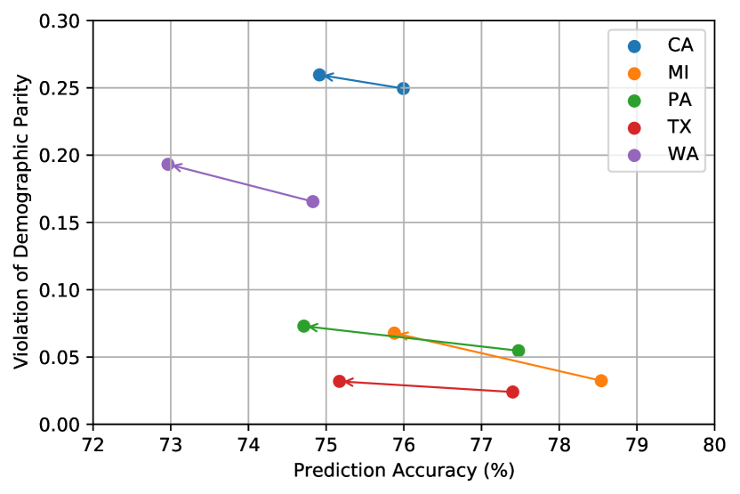
Figure 1: In Section 7, we evaluate our bounds against historical, temporal distribution shifts in demographics and income recorded by the US Census Bureau [13]. The above figure depicts changes to income-prediction accuracy and demographic parity violation when a classifier initially trained on US state-specific demographic data for 2014 is reused on 2018 data, thus exemplifying the negative potential effects of distribution shift.

Our primary result is a bound on a policy’s potential “violation of statistical group fairness”—defined in terms of the differences in policy outcomes between groups—when applied to a target distribution shifted relative to the source distribution within known constraints. Such settings naturally arise whenever training data represents a random sample of a target population with different statistics or a sample from dynamic environments, when a policy is reused on a new distribution without retraining, or whenever policy deployment itself induces a distribution shift. As an example of this last case, strategic individuals seeking loans might change their features or abstain from future application (thus shifting the distribution of examples) in response to policies trained on historical data [18, 38, 43]. Beyond policy selection, exogenous pressure such as economic trends and noise may also drive distribution shift in this example.

In Figure 1, we show how a real-world distribution shift in demographic and income data for US states between 2014 and 2018 may increase fairness violations while decreasing accuracy for a hypothetical classifier trained on the 2014 distribution. In such settings, it is useful to quantify how fairness guarantees transfer across distributions shifted within some bound, thus allowing the deployment of unfair machine learning policies to be avoided.

1.1 Related Work

Our work considers a setting similar to recent studies of domain adaptation, which have largely focused on characterizing the effects of distribution shift on prediction performance rather than fairness. Our work also builds on efforts in algorithmic fairness, especially dynamical treatments of distribution shift in response to deployed machine learning policies [23, 11, 30]. We reference specific prior work in these domains in Appendix B, and here discuss existing work that focuses on how certain measures of fairness are affected when policies are subject to specific distribution shift.

Fairness subject to Distribution Shift: A number of recent studies have considered specific examples of fairness transferability subject to distribution shift [34, 9, 36, 31, 21]. In particular, Schumann et al. [34] examine equality of opportunity and equalized odds as definitions of group fairness subject to distribution shifts quantified by an ${\mathcal{H}}$-divergence function; Coston et al. [9] consider demographic parity subject to a covariate shift assumption while group identification remains unavailable to the classifier; Singh et al. [36] focus on common group fairness definitions for binary classifiers subject to a class of distribution shift that generalizes covariate shift and label shift by preserving some conditional probability between variables; and Rezaei et al. [31] similarly consider common binary classification fairness definitions such as equalized odds subject to covariate shift. While we address similar settings to these works as special cases of our bound, we propose a unifying formulation for a broader class of statistical group fairness definitions and distribution shifts. In doing so, we recognize that particular settings recommend themselves to more natural measures of distribution shift, providing examples in Section 4.1, Section 4.2, and Section 5).

Another thread in existing literature is the development of robust models with the goal of guaranteeing fairness on a modelled target distribution (e.g., [1, 32, 26, 3, 21]) , for example, by assuming covariate shift and the availability of some unlabelled target data [9, 36, 31]. In particular, Singh et al. [36] focus on learning stable models that will preserve prediction accuracy and fairness, utilizing a causal graph to describe anticipated distribution shifts. Rezaei et al. [31] takes a robust optimization approach, and Coston et al. [9] develops prevalence-constrained and target-fair covariate shift method for getting the robust model. In contrast, our goal is to quantify fairness violations after an adversarial distribution shift for any given policy, including those not trained with robustness in mind.

1.2 Our Contributions

Our primary contribution is formulating a general, worst-case upper bound for a given policy’s violation of statistical group fairness subject to group-dependent distribution shifts within presupposed bounds (i.e., Equation 9). Bounding violations of fairness subject to distribution shift allows us to recognize and avoid potentially inappropriate deployments of machine learning when the potential disparities of a prospective policy eclipse a given threshold within bounded distribution shifts of the training distribution.

We first characterize the space of statistical group fairness definitions and possible distribution shifts by appeal to premetric functions (Definition 2.1). After formulating the worst-case upper bound, we explore common sets of simplifying assumptions for this bound as special cases, yielding tractable calculations for several familiar combinations of fairness definitions and subcases of distribution shift (Theorem 4.1, Theorem 5.2) with readily interpretable results. Finally, we compare our theoretical bounds to prescribed models of distribution shift in Section 6 and to real-world data in Section 7. The details for reproducing our experimental results can be found at
https://github.com/UCSC-REAL/Fairness_Transferability.

2 Formulation

The appendices include a table of notation (Appendix A) and all proofs (Appendix F).

2.1 Algorithmic Prediction

We consider two distributions, ${\mathcal{S}}$ (source) and ${\mathcal{T}}$ (target), each defined as a probability distribution for examples, where each example defines values for three random variables: $X$, a feature (e.g., $x$) with arbitrary domain $\mathcal{X}$; $Y$, a label (e.g., $y$) with arbitrary domain $\mathcal{Y}$; and $G$, a group (e.g., $g$ or $h$) with finite, countable domain $\mathcal{G}$. The predictor’s policy $\pi$, intended for ${\mathcal{S}}$ but used on ${\mathcal{T}}$, defines a fourth variable for each example: viz., $\hat{Y}$, a predicted label (e.g., $\hat{y}$) with domain $\hat{\mathcal{Y}}=\mathcal{Y}$.

Using $\mathcal{P}(\cdot)$ to denote the space of probability distributions over some domain, we denote the space of distributions over examples as $\mathds{D}\coloneqq\mathcal{P}(\mathcal{X}\times\mathcal{Y}\times\mathcal{G})$, such that ${\mathcal{S}},{\mathcal{T}}\in\mathds{D}$. It will also be useful for us to notate the space of distributions over example outcomes associated with a given policy as $\mathds{O}\coloneqq\mathcal{P}(\mathcal{X}\times\mathcal{Y}\times\hat{\mathcal{Y}})$ and the space of distributions over of group-specific examples as $\mathds{G}\coloneqq\mathcal{P}(\mathcal{X}\times\mathcal{Y})$.

Without loss of generality, we allow the prediction policy $\pi$ to be stochastic, such that, for any combination $(x,g)$, the predictor effectively samples $\hat{Y}$ from a corresponding probability distribution $\pi(x,g)$. Stochastic classifiers arise in various constrained optimization problems and proven useful for making problems with custom losses or fairness constraints tractable [10, 17, 29, 40].

We denote the space of nondeterministic policies as $\Pi\coloneqq(\mathcal{X}\times\mathcal{G}\to\mathcal{P}(\hat{\mathcal{Y}}))$ (e.g., $\pi\in\Pi$) and utilize the natural transformations that relate the spaces of distributions $\mathds{D}$, policies $\Pi$, and outcomes $\mathds{O}$:

$$\Pr_{\pi,{\mathcal{T}}}(\hat{Y}{=}\hat{y},X{=}x,G{=}g)=\Pr_{\hat{Y}\sim\pi(x,g)}(\hat{Y}{=}\hat{y})\cdot\Pr_{X,G\sim{\mathcal{T}}} (X{=}x,G{=}g)$$ (1)

We abuse the $\Pr$ notation for both probability density and probability mass functions as appropriate.

2.2 Statistical Group-Fairness

We next define a broad class of disparity functions ${\Delta^{\star}}\colon\Pi\times\mathds{D}\to\mathbf{R}$ representing how “unfair” a given policy is for a given distribution (e.g., writing ${\Delta^{\star}}(\pi,\mathcal{T})$), noting that this notion of fairness is limited to capturing statistical discrepancies of outcomes between groups.

Definition 2.1.

We define a premetric $\Psi$ on the space of distributions $p$ with respect to $q$ by the properties $\Psi(p\parallel q)\geq 0$ and $\Psi(p\parallel p)=0$ for all $p,q$, and refer to the value of $\Psi$ as a “shift”.

Definition 2.2.

We define a statistical group disparity ${\Delta^{\star}}$ for policy $\pi$ and distribution ${\mathcal{T}}$ in terms of the symmetrized shifts between group-specific outcome distributions. We measure shifts between outcome distributions with a given premetric $\Psi\colon\mathds{O}^{2}\to\mathbf{R}$.

$${\Delta^{\star}}(\pi,{\mathcal{T}})\coloneqq\sum_{g,h\in\mathcal{G}}\Psi\Big{(}\Pr_{\pi,{\mathcal{T}}}(X,Y,\hat{Y}\mid G{=}g)\leavevmode\nobreak\ \big{\|}\leavevmode\nobreak\ \Pr_{\pi,{\mathcal{T}}}(X,Y,\hat{Y}\mid G{=}h)\Big{)}$$ (2)

In Definition 2.2, $\Psi$ quantifies the specific statistical differences in outcomes between groups that are "unfair", where a value of 0 implies perfect fairness. In this work, we assume that $\Psi$ is the same for all $g,h$ and that ${\Delta^{\star}}$ is insensitive to relative group size $\Pr(G)$.

Examples

Familiar applications of Definition 2.2 include demographic parity (DP) and equalized odds (EO). A policy satisfying DP , in expectation, assigns a given binary classification $y\in\{0,1\}$ to the same fraction of examples in each group. We may measure the violation of DP as

$$\begin{multlined}{\Delta^{\star}}_{\textsf{DP}}(\pi,{\mathcal{T}})\coloneqq\sum_{g,h\in\mathcal{G}}\Big{|}\Pr_{\pi,{\mathcal{T}}}(\hat{Y}{=}1\mid G{=}g)-\Pr_{\pi,{\mathcal{T}}}(\hat{Y}{=}1\mid G{=}h)\Big{|}\end{multlined}{\Delta^{\star}}_{\textsf{DP}}(\pi,{\mathcal{T}})\coloneqq\sum_{g,h\in\mathcal{G}}\Big{|}\Pr_{\pi,{\mathcal{T}}}(\hat{Y}{=}1\mid G{=}g)-\Pr_{\pi,{\mathcal{T}}}(\hat{Y}{=}1\mid G{=}h)\Big{|}$$ (3)

The associated premetric $\Psi_{\textsf{DP}}$ for $p,q\in\mathds{O}$ is $\Psi_{\textsf{DP}}(p\parallel q)=\Big{|}\Pr_{p}(\hat{Y}{=}1)-\Pr_{q}(\hat{Y}{=}1)\Big{|}.$

To satisfy EO, for binary $\mathcal{Y}=\{0,1\}$, $\pi$ must maintain group-invariant true positive and false positive classification rates. We may measure the violation of EO as

$${\Delta^{\star}}_{\textsf{EO}}(\pi,{\mathcal{T}})\coloneqq\sum_{g,h\in\mathcal{G}}\sum_{y\in\mathcal{Y}}\Big{|}\Pr_{\pi,{\mathcal{T}}}(\hat{Y}{=}1\mid G{=}g,Y{=}y)-\Pr_{\pi,{\mathcal{T}}}(\hat{Y}{=}1\mid G{=}h,Y{=}y)\Big{|}$$ (4)

The associated premetric is $\Psi_{\textsf{EO}}(p\parallel q)=\sum_{y\in\mathcal{Y}}\Big{|}\Pr_{p}(\hat{Y}{=}1\mid Y{=}y)-\Pr_{q}(\hat{Y}{=}1\mid Y{=}y)\Big{|}.$ Note that the restriction of EO to the $(Y=1)$ case is known as Equal Opportunity (EOp).

We remark that Definition 2.2 provides a unifying representation for a wide array of statistical group “unfairness” definitions and may be used with inequality constraints. That is, we may recover many working definitions of fairness that effectively specify a maximum value of disparity:

Definition 2.3.

A policy $\pi$ is $\bm{\epsilon}$-fair with respect to ${\Delta^{\star}}$ on distribution ${\mathcal{T}}$ iff ${\Delta^{\star}}(\pi,{\mathcal{T}})\leq\epsilon$.

2.3 Vector-Bounded Distribution Shift

Suppose, after developing policy $\pi$ for distribution ${\mathcal{S}}$, we realize some new distribution ${\mathcal{T}}$ on which the policy is actually operating. This realization may be the consequence of sampling errors during the learning process, strategic feedback to our policy, random processes, or the reuse of our policy on a new distribution for which retraining is impractical. Our goal is to bound ${\Delta^{\star}}(\pi,{\mathcal{T}})$ given knowledge of ${\Delta^{\star}}(\pi,{\mathcal{S}})$ and some notion of how much ${\mathcal{T}}$ possibly differs from $S$.

Definition 2.4.

$K(p\parallel q)$ is a divergence if and only if for all $p$ and $q$, $K(p\parallel q)\geq 0$ and $K(p\parallel q)=0\iff q=p$.

Definition 2.5.

Define the group-vectorized shift $\mathbf{D}$, as ${\mathcal{S}}$ mutates into ${\mathcal{T}}$, as

$$\mathbf{D}({\mathcal{T}}\parallel{\mathcal{S}})\coloneqq\sum_{g}\mathbf{e}_{g}D_{g}\big{(}\Pr_{{\mathcal{T}}}(X,Y\mid G{=}g)\parallel\Pr_{{\mathcal{S}}}(X,Y\mid G{=}g)\big{)}$$ (5)

where $\mathbf{e}_{g}$ represents a unit vector indexed by $g$, and each $D_{g}\colon\mathds{G}^{2}\to\mathbf{R}$ is a divergence (Definition 2.4). Note that each $D_{g}$ also defines a premetric (but not necessarily a divergence) on $\mathds{D}$.

Assumption 2.6.

Let there exist some vector $\mathbf{B}\succeq 0$ bounding $\mathbf{D}({\mathcal{T}}\parallel{\mathcal{S}})\preceq\mathbf{B}$, where $\preceq$ and $\succeq$ denote element-wise inequalities.

In 2.6, $\mathbf{B}$ limits the possible distribution shift as ${\mathcal{S}}$ mutates into ${\mathcal{T}}$, without requiring us to specify a model for how distributions evolve. When modelling distribution shift requires complex dynamics (e.g., when agents learn and respond to classifier policy), we reduce a potentially difficult dynamical problem to a more tractable, adversarial problem to achieve a bound.

Lemma 2.7.

For all $\pi$, ${\Delta^{\star}}$, and $\mathbf{D}$, when $\mathbf{B}=0$, ${\Delta^{\star}}(\pi,{\mathcal{S}})={\Delta^{\star}}(\pi,{\mathcal{T}})$.

Lemma 2.7 indicates that, for a fixed policy $\pi$, a change in disparity requires a measurable shift in distributions from ${\mathcal{S}}$ to ${\mathcal{T}}$, confirming intuition.

Restricted Distribution Shift

Common assumptions that restrict the set of distribution shifts include covariate shift and label shift. For covariate shift, the distribution of labels conditioned on features is preserved across distributions for all groups, while for label shift, the distributions of features conditioned on labels is preserved across distributions for all groups.

Covariate shift implies $$\Pr_{{\mathcal{T}}}(Y\mid X,G)=\Pr_{{\mathcal{S}}}(Y\mid X,G)$$ (6)

Label shift implies $$\Pr_{{\mathcal{T}}}(X\mid Y,G)=\Pr_{{\mathcal{S}}}(X\mid Y,G)$$ (7)

In Section 4, we explore a deterministic model of a population’s response to classification as an example of covariate shift. We do the same in Section 5 for label shift.

3 General Bounds

We first define a primary bound in Definition 3.1 before considering simplifying special cases.

Given an element-wise bound $\mathbf{B}$ on the vector-valued shift $\mathbf{D}({\mathcal{T}}\parallel{\mathcal{S}})$ (2.6) we may bound the disparity ${\Delta^{\star}}$ of policy $\pi$ on any realizable target distribution ${\mathcal{T}}$ by its supremum value.

Definition 3.1.

Define the supremum value $v$ for ${\Delta^{\star}}$ subject to $\mathbf{D}({\mathcal{T}}\parallel{\mathcal{S}})\preceq\mathbf{B}$ as

$$v({\Delta^{\star}},\mathbf{D},\pi,{\mathcal{S}},\mathbf{B}) \coloneqq\sup_{\mathbf{D}({\mathcal{T}}\parallel{\mathcal{S}})\preceq\mathbf{B}}{\Delta^{\star}}(\pi,{\mathcal{T}})$$ (8)

$$\mathbf{D}({\mathcal{T}}\parallel{\mathcal{S}})\preceq\mathbf{B} \implies{\Delta^{\star}}(\pi,{\mathcal{T}})\leq v({\Delta^{\star}},\mathbf{D},\pi,{\mathcal{S}},\mathbf{B})$$ (9)

In general, our strategy is to exploit the mathematical structure of the setting encoded by ${\Delta^{\star}}$ (i.e., $\Psi$) and $\mathbf{D}$ to obtain an upper bound for $v$ defined in Equation 8. We first explore general cases of simplifying assumptions before presenting worked special examples for frequently encountered settings. Finally, we compare the resulting theoretical bounds to numerical results and simulations.

3.1 Lipshitz Conditions

The value of $v$ defines a scalar field in $\mathbf{B}$ and therefore a conservative vector field $\mathbf{F}=\nabla_{\mathbf{B}}v$.

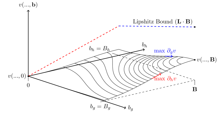
Figure 2: A Lipshitz bound for all curves parameterized by distribution shift bound $\mathbf{b}$ in the $(0,\mathbf{B})$ $\mathds{D}$-hyperrectangle on the surface $v$. In the figure, for groups $i\in\{g,h\}$, $\max\partial_{i}v=L_{i}$, and the colored dotted lines corresponds to $L_{i}b_{i}$, which, when summed, equal $\mathbf{L}\cdot\mathbf{B}$.

For any curve in $\mathds{D}$ from ${\mathcal{S}}$ to ${\mathcal{T}}$, bounds of the form $\mathbf{F}\preceq\mathbf{L}$ for some constant $\mathbf{L}$ along the curve imply a Lipshitz bound on ${\Delta^{\star}}$. We visualize a bound in Figure 2 for all possible curves in the region $\mathbf{D}({\mathcal{T}}\parallel{\mathcal{S}})\preceq\mathbf{B}$.

Theorem 3.2 (Lipshitz Upper Bound).

If there exists an $\mathbf{L}$ such that $\nabla_{\mathbf{b}}v({\Delta^{\star}},\mathbf{D},\pi,{\mathcal{S}},\mathbf{b})\preceq\mathbf{L}$, everywhere along some curve as $\mathbf{b}$ varies from $0$ to $\mathbf{B}$, then

$${\Delta^{\star}}(\pi,{\mathcal{T}})\leq{\Delta^{\star}}(\pi,{\mathcal{S}})+\mathbf{L}\cdot\mathbf{B}$$ (10)

Succinctly, if we are guaranteed that disparity can never increase faster than a certain rate in some measure of distribution shift, then, given a maximum distribution shift, this rate bounds the maximum possible disparity. The utility of Theorem 3.2 arises when a Lipshitz condition $\mathbf{L}$ is known, but direct computation of $v$ is difficult. We provide an example of a Lipshitz bound in Section 5.

3.2 Subadditivity Conditions

Definition 3.3.

Define $w$ as the maximum increase in disparity subject to $\mathbf{D}({\mathcal{T}}\parallel{\mathcal{S}})\preceq\mathbf{B}$, i.e., $w({\Delta^{\star}},\mathbf{D},\pi,{\mathcal{S}},\mathbf{B})\coloneqq v({\Delta^{\star}},\mathbf{D},\pi,{\mathcal{S}},\mathbf{B})-{\Delta^{\star}}(\pi,{\mathcal{S}})$.

Theorem 3.4.

Suppose, in the region $\mathbf{D}({\mathcal{T}}\parallel{\mathcal{S}})\preceq\mathbf{B}$, that $w$ is subadditive in its last argument. That is, $w(...,\mathbf{a})+w(...,\mathbf{c})\geq w(...,\mathbf{a}+\mathbf{c})$ for $\mathbf{a},\mathbf{c}\succeq 0$ and $\mathbf{a}+\mathbf{c}\preceq\mathbf{B}$. If $w$ is also locally differentiable, then a first-order approximation of $w(...,\mathbf{b})$ evaluated at $0$, i.e.,

$$\mathbf{L}=\nabla_{\mathbf{b}}w(...,\mathbf{b})\big{|}_{\mathbf{b}=0}=\nabla_{\mathbf{b}}v(...,\mathbf{b})\big{|}_{\mathbf{b}=0}$$ (11)

provides an upper bound for $v(...,\mathbf{B})$, i.e.,

$$v({\Delta^{\star}},\mathbf{D},\pi,{\mathcal{S}},\mathbf{B})\leq{\Delta^{\star}}(\pi,{\mathcal{S}})+\mathbf{L}\cdot\mathbf{B}$$ (12)

Theorem 3.4 notes that “diminishing returns” in the change of ${\Delta^{\star}}$ as the difference of ${\mathcal{T}}$ with respect to ${\mathcal{S}}$ is increased implies a bound on ${\Delta^{\star}}$ in terms of its local sensitivity to $\mathbf{D}$ at ${\mathcal{S}}$ (i.e., using a first-order Taylor approximation). Note that, if $w$ is concave in the bounded region, it is also subadditive in the bounded region, but the converse is not true, nor does the converse imply Lipshitzness.

3.3 Geometric Structure

It may happen that $\Psi\colon\mathds{O}^{2}\to\mathbf{R}$ and each $D_{g}\colon\mathds{G}^{2}\to\mathbf{R}$ share structure that permits a geometric interpretation of distribution shift. While the utility of this observation depends on the specific properties of $\Psi$ and $\mathbf{D}$, we demonstrate a worked example building on Section 4.2 in Appendix D, in which we allow ourselves to select a suitable $\mathbf{D}$ for ease of interpretation. We proceed to consider worked examples that adopt common assumptions limiting the form of distribution shift and apply common definitions of statistical group fairness.

4 Covariate Shift

We now present our fairness transferability results subject to covariate shift for both demongraphic parity (Section 4.1) and equalized opportunity (Section 4.2) as fairness criteria.

4.1 Demographic Parity

The simplest way to work with Equation 8 is to bound the supremum $v$. We first consider demographic parity (Equation 3) for $\mathcal{Y}=\{0,1\}$ and $\mathcal{G}=\{g,h\}$, subject to covariate shift (Equation 6). We find that the form of ${\Delta^{\star}_{{\textsf{DP}}}}$ subject to covariate shift recommends itself to a natural choice of vector divergence, $\mathbf{D}$. First, define a re-weighting coefficient $\omega_{g}({\mathcal{T}},{\mathcal{S}},x)\coloneqq\frac{\Pr_{{\mathcal{T}}}(X{=}x\mid G{=}g)}{\Pr_{{\mathcal{S}}}(X{=}x\mid G{=}g)}$.

Theorem 4.1.

For demographic parity between two groups under covariate shift (denoting, for each $g$, $\beta_{g}\coloneqq\Pr_{\pi,{\mathcal{S}}}(\hat{Y}{=}1\mid G{=}g)$),

$${\Delta^{\star}}_{{\textsf{DP}}}(\pi,{\mathcal{T}})\leq{\Delta^{\star}}_{{\textsf{DP}}}(\pi,{\mathcal{S}})+\sum_{g}\big{(}\beta_{g}(1-\beta_{g})\cdot\operatorname*{Var}_{{\mathcal{S}}}[\omega_{g}({\mathcal{T}},{\mathcal{S}},x)]\big{)}^{\nicefrac{{1}}{{2}}}$$ (13)

We notice that $\operatorname*{Var}_{{\mathcal{S}}}[\omega_{g}({\mathcal{T}},{\mathcal{S}},x)]$ recommends itself as a suitable divergence $D_{g}$ from ${\mathcal{S}}$ to ${\mathcal{T}}$. Using basis vectors $\mathbf{e}_{g}$, for this example, we could define $\mathbf{D}(\mathcal{T}\parallel{\mathcal{S}})=\sum_{g}\mathbf{e}_{g}\operatorname*{Var}_{{\mathcal{S}}}[\omega_{g}(\mathcal{T},{\mathcal{S}},x)]$. When $\operatorname*{Var}_{{\mathcal{S}}}[\omega_{g}({\mathcal{T}},{\mathcal{S}},x)]\leq B_{g}$, it follows ${\Delta^{\star}}_{{\textsf{DP}}}(\pi,{\mathcal{T}})\leq{\Delta^{\star}}_{{\textsf{DP}}}(\pi,{\mathcal{S}})+\sum_{g}\big{(}\beta_{g}(1-\beta_{g})\cdot B_{g}\big{)}^{\nicefrac{{1}}{{2}}}$. Comparing the inequality in Theorem 4.1 and the consequent of Equation 10, we can interpret $\Pr_{\pi,{\mathcal{S}}}(\hat{Y}{=}1)$ in Theorem 4.1 as an upper bound for the average value of $\nabla_{\mathbf{b}}v({\Delta^{\star}}_{\textsf{DP}},\mathbf{D},\pi,{\mathcal{T}},\mathbf{b})$ along any curve from ${\mathcal{S}}$ to ${\mathcal{T}}$. Interpreting this result, the closer ${\rm Pr}(\hat{Y}{=}1)$ is to 0.5 for any group, the more potentially sensitive the fairness of the policy is to distribution shifts for that group. We can further generalize the results to multi-class and multi-group setting:

Corollary 4.2.

Theorem 4.1 may be generalized to multiple classes $\mathcal{Y}=\{1,2,...,m\}$ and multiple groups $\mathcal{G}\in\{1,2,...,n\}$, where $\beta_{g,y}=\Pr(\hat{Y}{=}y\mid G{=}g)$ and assuming $\operatorname*{Var}_{{\mathcal{S}}}[\omega_{g}({\mathcal{T}},{\mathcal{S}},x)]\leq B_{g}$:

$${\Delta^{\star}_{{\textsf{DP}}}}(\pi,{\mathcal{T}}) \coloneqq\sum_{y\in\mathcal{Y}}\sum_{g,h\in\mathcal{G}}\Big{|}\Pr_{\pi,{\mathcal{T}}}(\hat{Y}{=}y\mid G{=}g)-\Pr_{\pi,{\mathcal{T}}}(\hat{Y}{=}y\mid G{=}h)\Big{|}$$ (14)

$${\Delta^{\star}}_{{\textsf{DP}}}(\pi,{\mathcal{T}}) \leq{\Delta^{\star}}_{{\textsf{DP}}}(\pi,{\mathcal{S}})+\sum_{y}\sum_{g}\big{(}\beta_{g,y}(1-\beta_{g,y})\cdot B_{g}\big{)}^{\nicefrac{{1}}{{2}}}$$ (15)

We remark that in general, binary classification bounds may frequently be generalized to multi-class bounds by redefining fairness violations as a sum of binary-class fairness violations (i.e., same-class vs. different-class labels) and summing the bounds on each.

4.2 Equal Opportunity

Consider an example using the $(Y{=}1)$-conditioned case of Equalized Odds—termed Equal Opportunity (EOp). Denoting, for each group $g$, the true positive rate $\beta^{+}_{g}\coloneqq\Pr_{\pi,{\mathcal{T}}}(\hat{Y}{=}1\mid Y{=}1,G{=}g)$ as an implicit function of $\pi$ and ${\mathcal{T}}$, we define disparity for EOp as ${\Delta^{\star}}_{\textsf{EOp}}(\pi,{\mathcal{T}})\coloneqq\sum_{g,h\in\mathcal{G}}|\beta^{+}_{g}-\beta^{+}_{h}|$.

We may bound the realized value of ${\Delta^{\star}}_{{\textsf{EOp}}}(\pi,{\mathcal{T}})$ by bounding $\beta^{+}_{g}$ for each group:

Theorem 4.3.

Subject to covariate shift and any given $\mathbf{D},\mathbf{B}$, assume extremal values for $\beta_{g}^{+}$, i.e.,

$$\forall g,\leavevmode\nobreak\ \leavevmode\nobreak\ \big{(}D_{g}({\mathcal{T}}\parallel{\mathcal{S}})<B_{g}\big{)}\implies\big{(}l_{g}\leq\beta^{+}_{g}(\pi,{\mathcal{T}})\leq u_{g}\big{)}$$ (16)

it follows that

$$v({\Delta^{\star}}_{{\textsf{EOp}}},\mathbf{D},\pi,{\mathcal{S}},\mathbf{B})\leq\max_{\begin{subarray}{c}{x_{g}\in\{l_{g},u_{g}\}}\\ {x_{h}\in\{l_{h},u_{h}\}}\end{subarray}}\sum_{g,h}\Big{|}x_{g}-x_{h}\Big{|}$$ (17)

Corollary 4.4.

The disparity measurement ${\Delta^{\star}}_{\textsf{EOp}}$ cannot exceed $\frac{|\mathcal{G}|^{2}}{4}$.

In Appendix D, we bound the extremal values of $\beta_{g}^{+}$ by geometrically interpreting this quantity as an inner product on an appropriate vector space, utilizing the freedom to select an appropriate $\mathbf{D}$.

5 Label Shift

Under label shift ($\Pr_{\mathcal{S}}(X|Y)=\Pr_{\mathcal{T}}(X|Y)$), violations of EO and EOp are invariant, because the independence of $\hat{Y}$ and $Y$ given $X$ implies $\Pr_{\pi,{\mathcal{T}}}(\hat{Y}|Y)=\Pr_{\pi,{\mathcal{S}}}(\hat{Y}|Y)$. We therefore focus on the violation of demographic parity (DP) (Equation 3) subject to the label shift condition, treating a binary classification task over two groups for simplicity.

In this setting, we choose to measure group-specific distribution shifts from ${\mathcal{S}}$ to ${\mathcal{T}}$ by the change in proportion of ground-truth positive labels, which we refer to as the group qualification rate $Q_{g}({\mathcal{T}})\coloneqq\Pr_{\mathcal{T}}(Y=1\mid G=g)$:

$$D_{g}({\mathcal{T}}\parallel{\mathcal{S}})\coloneqq\Big{|}Q_{g}(\mathcal{S})-Q_{g}(\mathcal{{\mathcal{T}}})\Big{|}\leq B_{g}$$ (18)

Theorem 5.1.

A Lipshitz condition bounds $\nabla_{\mathbf{b}}v({\Delta^{\star}}_{\textsf{DP}},\mathbf{D},\pi,{\mathcal{S}},\mathbf{b})$ when

$$D_{g}({\mathcal{T}}\parallel{\mathcal{S}})\coloneqq\Big{|}Q_{g}(\mathcal{S})-Q_{g}(\mathcal{{\mathcal{T}}})\Big{|}\leq B_{g}$$ (19)

Specifically,

$$\partialderivative{b_{g}}v({\Delta^{\star}}_{\textsf{DP}},\mathbf{D},\pi,{\mathcal{S}},\mathbf{b})\leq(|\mathcal{G}|-1)\Big{|}\beta^{+}_{g}-\beta^{-}_{g}\Big{|}$$ (20)

for true positive rates $\beta^{+}_{g}$ and false positive rates $\beta^{-}_{g}$:

$$\beta^{+}_{g}\coloneqq\Pr_{\pi}(\hat{Y}{=}1\mid Y{=}1,G{=}g);\quad\beta^{-}_{g}\coloneqq\Pr_{\pi}(\hat{Y}{=}1\mid Y{=}0,G{=}g)$$ (21)

Because $\beta^{+}_{g}$ and $\beta^{-}_{g}$ are invariant under label shift given a constant policy $\pi$, we elide their explicit dependence on the underlying distribution.

Theorem 5.2.

For DP under the bounded label-shift assumption $\forall g,|Q_{g}({\mathcal{S}})-Q_{g}({\mathcal{T}})|\leq B_{g}$,

$${\Delta^{\star}_{{\textsf{DP}}}}(\pi,{\mathcal{T}}) \leq{\Delta^{\star}_{{\textsf{DP}}}}(\pi,{\mathcal{S}})+(|\mathcal{G}|-1)\sum_{g}B_{g}\ \Big{|}\beta^{+}_{g}-\beta^{-}_{g}\Big{|}$$ (22)

Intuitively, the change in ${\Delta^{\star}}_{\textsf{DP}}$ subject to label shift depends on $|\beta^{+}_{g}-\beta^{-}_{g}|$, the marginal change in acceptance rates as agents change their qualifications $Y$. We measure the distribution shift as agents change their qualifications by $|Q_{g}({\mathcal{S}})-Q_{g}({\mathcal{T}})|$. When $\beta^{+}_{g}$ is close to $\beta^{-}_{g}$, the policy looks like a random classifier, and a label shift has limited effect on statistical group disparity. When $|\beta^{+}_{g}-\beta^{-}_{g}|$ is large, indicating high classifier accuracy, the effect on supremal disparity is larger. Our bound thus exposes a direct trade-off between accuracy and fairness transferability guarantees.

6 Comparisons to Synthetic Distribution Shifts (Demographic Parity)

To further interpret our results, in this section, we consider specific and popular agent models to characterize distribution shift and instantiate our bounds for particular forms of $\mathbf{D}$, $\mathbf{B}$, and ${\Delta^{\star}}$.

6.1 Covariate Shift via Strategic Response

Let us consider a specific example of covariate shift (Equation 6) caused by a deterministic, group-independent model of strategic response in which agents react to a binary classification policy $\pi$ characterized by group-specific feature thresholds:

$$\hat{Y}\sim\pi(x,g)=\begin{cases}1&\text{ with probability }1\text{ if }x\geq\tau_{g}\\ 0&\text{ with probability }1\text{ otherwise }\end{cases}$$ (23)

For simplicity, we assume the feature domain $\mathcal{X}=[0,1]$. In response to threshold $\tau_{g}$, agents in each group $g$ may modify their feature $x$ to $x^{\prime}$ by incurring a cost $c_{g}(x,x^{\prime})\geq 0$. Similar to [18], we define the utility $u_{g}$ for agents in group $g$ to be

$$u_{g}(x,x^{\prime}) \coloneqq\beta_{g}(x^{\prime})-\beta_{g}(x)-c_{g}(x,x^{\prime});\quad\beta_{g}(x)\coloneqq\Pr(\hat{Y}{=}1\mid X{=}x,G{=}g),\forall g.$$ (24)

Contrary to the standard strategic classification setting, we do not assume that feature updates represent false reports, but that such updates may correspond to actual changes underlying the true qualification $Y$ of each agent. This assumption has been made in a recent line of research in incentivizing improvement from human agents subject to such classification [5].

Next, we assume all agents are rational utility maximizers (Equation 24). For a given threshold $\tau_{g}$ and manipulation budget $m_{g}$, the best response of an agent with original feature $x$ is

$$x^{\prime}=\operatorname*{argmax}_{z}\ u_{g}(x,z),\quad\text{ such that }\ c_{g}(x,z)\leq m_{g}$$ (25)

To make the problem tractable, we make additional assumptions about the agents’ best responses.

Assumption 6.1.

An agent’s original feature $x$ is sampled as $X\sim\mathcal{U}_{[0,1]}$.

Assumption 6.2.

The cost function $c_{g}(x,x^{\prime})$ is monotone in $|x-x^{\prime}|$ as $c_{g}(x,x^{\prime})=|x^{\prime}-x|$.

Under 6.2, only those agents with features $x\in[\tau_{g}-m_{g},\tau_{g})$ will attempt to change their feature. We also assume that feature updates are non-deterministic, such that agents with features closer to the decision boundary $\tau_{g}$ have a greater chance of updating their feature and each updated feature $x^{\prime}$ is sampled from a uniform distribution depending on $\tau_{g}$, $m_{g}$, and $x$:

Assumption 6.3.

For agents who attempt to update their features, the probability of a successful feature update is $\Pr(X\neq X^{\prime})=1-\frac{|x-\tau_{g}|}{m_{g}}$.

Assumption 6.4.

An agent’s updated feature $x^{\prime}$, given original feature $x$, manipulation budget $m_{g}$, and classification boundary $\tau_{g}$, is sampled as $X^{\prime}\sim\mathcal{U}_{[\tau_{g},\tau_{g}+m_{g}-x]}$.

With the above setting, we can specify the reweighting coefficient $\omega_{g}(x)$ for our setting (Equation 102 in Section F.1 and get the following bound for the strategic response setting:

Proposition 6.5.

For our assumed setting of strategic response involving DP for two groups $\{g,h\}$, Theorem 4.1 implies

$${\Delta^{\star}_{{\textsf{DP}}}}(\pi,{\mathcal{T}})\leq{\Delta^{\star}_{{\textsf{DP}}}}(\pi,{\mathcal{S}})+\tau_{g}(1-\tau_{g})\frac{2}{3}m_{g}+\tau_{h}(1-\tau_{h})\frac{2}{3}m_{h}$$ (26)

The above result shows that two factors lead to a smaller difference between the source and target fairness violations: a less stochastic classifier (when the threshold $\tau_{g}$ is far away from $0.5$) and a smaller manipulation budget $m_{g}$ (diminishing agents’ ability to adapt their feature). In this case, $B_{g}=\frac{2}{3}\tau_{g}(1-\tau_{g})$. These factors lead to less potential manipulation and result in a tighter upper bound for the fairness violation on ${\mathcal{T}}$.

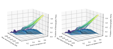
(a) A stereoscopic (cross-eye view) comparison between the bound of Section 4.1 (gradated) and simulated results for the model of Section 6.1 (blue) in response to a DP-fair classifier with different initial group-independent acceptance rates.

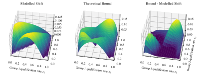
(b) A policy satisfying DP is subject to distribution shift prescribed by replicator dynamics (Section 6.2). Realized disparity increases (blue) are compared to the theoretical bound (Theorem 5.2, gradated), which is tight when group have dissimilar qualification rates.

Figure 3: Comparisons to synthetic distribution. Larger versions are provided in Appendix E.

6.2 Label Shift via Replicator Dynamics

We now evaluate our theoretical bound for demographic parity subject to label shift (Theorem 5.2) on the replicator dynamics model of Raab and Liu [30]. Briefly, replicator dynamics assumes that the proportion of agents in a population choosing one strategy over another grows in proportion to the ratio of average utilities realized by the two strategies. The cited model additionally assumes $\mathcal{X}=\mathbf{R}$, $\mathcal{Y}=\{{0,1}\}$, and a monotonicity condition for ${\mathcal{S}}$ given by $\derivative{x}\frac{\Pr_{{\mathcal{S}}}(X{=}x\mid Y{=}1)}{\Pr_{{\mathcal{S}}}(X{=}x\mid Y{=}0)}>0$.

Label shift under the discrete-time ($t$) replicator dynamics may be expressed in terms of group qualification rates $Q_{g}\coloneqq\Pr_{t}(Y{=}1\mid G{=}g)$ and agent utilities (i.e., group- and feature-independent values $U_{y,\hat{y}}$) such that, in each group, the popularity and average utility associated with a label determines its frequency at the next time step $t{+}1$.

Denote the fractions of group-conditioned, feature-independent outcomes with the expression $\rho^{y,\hat{y}}_{g}\coloneqq\Pr_{t}(\hat{Y}{=}\hat{y},Y{=}y\mid G{=}g)$ and abbreviate the fraction-weighted utility as $u^{y,\hat{y}}_{g}(t)\coloneqq U_{y,\hat{y}}\cdot\rho^{y,\hat{y}}_{g}$. We may then represent the replicator dynamics as

$$Q_{g}[t+1] =\frac{u^{{1,1}}_{g}(t)+u^{{1,0}}_{g}(t)}{u^{{1,1}}_{g}(t)+u^{{1,0}}_{g}(t)+u^{{0,0}}_{g}(t)+u^{{0,1}}_{g}(t)}$$ (27)

To apply Theorem 5.2, we also observe that $|\beta^{+}_{g}-\beta^{-}_{g}|=\frac{|\rho^{{1,1}}_{g}-\rho^{{0,1}}_{g}|}{\rho^{{1,1}}_{g}+\rho^{{0,1}}_{g}},$ where $\beta^{+}_{g}$ and $\beta^{-}_{g}$ represent the true positive rate and false positive rate for group $g$, respectively, and we use the change in qualification rate as our measurement of label shift, i.e., $B_{g}=|Q_{g}[t+1]-Q_{g}[t]|$. When demographic parity is perfectly satisfied, we note that the acceptance rate ($\rho^{{1,1}}_{g}+\rho^{{0,1}}_{g}$) is group-independent.

Theorem 6.6.

For DP subject to label replicator dynamics,

$${\Delta^{\star}_{{\textsf{DP}}}}(\pi,{\mathcal{T}})\leq{\Delta^{\star}_{{\textsf{DP}}}}(\pi,{\mathcal{S}})+\sum_{g}\Big{|}Q_{g}[t+1]-Q_{g}[t]\Big{|}\frac{|\rho^{{1,1}}_{g}-\rho^{{0,1}}_{g}|}{\rho^{{1,1}}_{g}+\rho^{{0,1}}_{g}}$$ (28)

In Figure 3(b), we graphically represent all possible states of an initially fair system (thus determining $\beta$ and $\rho$ as a result of the monotonicity condition) by the tuple of qualification rates for each group. With the dynamics prescribed by Equation 27, we depict the rate of change of disparity given a fixed, locally DP-fair policy, and compare this to the theoretical bound when $B_{g}=|Q_{g}[t+1]-Q_{g}[t]|$.

Interpreting our results, we note that the bound lacks information about the relative directions of the change in acceptance rates for each group, and thus over-approximates possible fairness violations when group acceptance rates shift the same direction. When group acceptance rates move in opposing directions, however, the bound gives excellent agreement with the modelled replicator dynamics.

7 Comparisons to Real-World Distribution Shifts

We now compare our special-case theoretical bounds (i.e., label/covariate shift) to real-world distribution shifts and hypothetical classifiers. We use American Community Survey (ACS) data provided by the US Census Bureau [16]. We adopt the sampling and pre-processing approaches following the Folktables package provided by Ding et al. [13] to obtain 1,599,229 data points. The data is partitioned by (1) all fifty US states and (2) years from 2014 to 2018. We use 10 features covering the demographic information used in the UCI Adult dataset [4], including age, occupation, education, etc., as $X$ for our model, select sex as binary protected group, i.e., $G\in\{g=\texttt{female},h=\texttt{male}\}$. We set the label $Y$ to whether an individual’s annual income is greater than $50K.

To apply our label-shift or covariate-shift bounds, we first need to verify whether the two datasets satisfy either of these assumptions. We adopted a conditional independence test [22], which takes data from source and target domains as input and returns a divergence score for each covariate and label variable, reflecting to what extent the variable is shifted between distributions. We find that the likelihood that the covariates shift across US states is approximately two orders of magnitude higher than for labels. More specifically, there are 4 covariates, including class of worker (probabilistic divergence score of 2.67e-2), hours worker per week (3.56e-2), sex (3.56e-2) and race (2.55e-1), that are more likely to be shifted than the label variable (1.29e-4). For temporal shifts within states, we find that the label variable is more likely to be shifted (0.1) than all the other covariates (which are below 0.01), approximately two orders of magnitude in favor of label shift over covariate shift. We therefore compare the disparities of hypothetical policies on these distributions to bounds generated from the corresponding, approximately satisfied assumptions.

On this data, we train a set of group-dependent, linear threshold classifiers $\Pr_{\pi(x,g)}(\hat{Y}{=}1)=\mathds{1}[\sigma(w\cdot x)>\tau_{g}]$, for a range of thresholds $\tau_{g}$ and $\tau_{h}$ for each source distribution. Here, $\sigma(\cdot)$ is the logistic function and $w$ denotes a weight vector. We then consider two types of real-world distribution shift: (1) geographic, in which a model trained for one state is evaluated on other US state in the same year, and (2) temporal, in which a model trained for 2014 is evaluated on the same state in 2018.

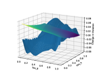
(a) CA $\longrightarrow$ IL

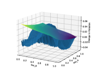
(b) CA $\longrightarrow$ NV

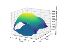
(c) CA: 2014 $\rightarrow$ 2018

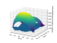
(d) TX: 2014 $\rightarrow$ 2018

Figure 4: Simulated change in DP violation (blue mesh) subject to geographic and temporal distribution shifts vs. direct application of bounds for approximately satisfied assumptions (respectively, Theorem 4.1 and Theorem 5.2) (gradated mesh). The $x$-axis and $y$-axis of both figures represent the policy thresholds $\tau_{g}$ and $\tau_{h}$.

We graphically compare the theoretical bounds of Theorem 4.1 and Theorem 5.2 for the increased violation of DP subject to covariate and label shift, respectively, to the simulated violations for our model and data in Figure 4. We provide additional examples and an evaluation of bounds for EO subject to covariate shift (noting that label shift preserves EO in theory) in Section E.2. Despite the fact that geographic or temporal distribution shifts only approximately satisfy the assumptions of covariate or label shift, these comparisons demonstrate that our theoretical bounds are not vacuous, approximately bounding the change of fairness violation across real-world domain shifts. For geographic shifts, the covariate shift EO bounds (Section E.2) correctly overestimate disparity and tighten near accurate policies, while our DP bounds are useful only for a subset of policy thresholds (Figure 4(b)). add specific pointer. e.g, 4.a, that one is 4.b For temporal shift, the label shift bound for DP correctly overestimates the real change of DP violations but still remains at the same order of magnitude (Figure 4(c) and 4(d)).

8 Conclusion and Discussion

In this paper, we have developed a unifying framework for bounding the violation of statistical group fairness guarantees when the underlying distribution shifts within presupposed bounds. We hope that this work can generate meaningful discussion regarding the viability of fairness guarantees subject to distribution shift, the bounds of adversarial attacks against algorithmic fairness, and evaluations of robustness with respect to algorithmic fairness. We believe that, just as published empirical measurements are of limited use without reported uncertainties, fairness guarantees must be accompanied by bounds on their robustness to distribution shift.

Future work remains to apply our framework for to problem of fairness transferability in settings with more complicated distribution shift dynamics. For example, compound distribution shifts [33], which compose covariate shifts and label shifts, cannot be treated by composing the theoretical bounds developed herein without additional information regarding intermediate distributions. Another potential future direction is to develop reasonable bounds on anticipated distribution shift from models of human behavior and exogenous pressures.

Acknowledgement

This work is supported by the National Science Foundation (NSF) under grants IIS-2143895, IIS-2040800 (FAI program in collaboration with Amazon), and CCF-2023495.

Appendix A Notation

Symbol	Usage
$X$	A random variable representing an example’s features.
$\mathcal{X}$	The domain of features $X$.
$Y$	A random variable representing an example’s ground truth label.
$\mathcal{Y}$	The domain of labels $Y$.
$\hat{Y}$	A random variable representing the predicted label for an example.
$\hat{\mathcal{Y}}$	The domain of predicted labels $\hat{Y}$ (distinguished semantically from $\mathcal{Y}$).
$G$	A random variable representing an example’s group membership.
$\mathcal{G}$	The domain for group membership $G$.
$\pi$	A learned (non-deterministic) policy for predicting $\hat{Y}$ from $X$ and $G$.
$\Pr$	A sample probability (density) according to a referenced distribution.
$\mathcal{P}$	The space of probability distributions over a given domain.
$\mathds{D}$	The space of distributions of examples over $\mathcal{X}\times\mathcal{Y}\times\mathcal{G}$.
$\mathds{O}$	The space of distributions of outcomes over $\mathcal{X}\times\mathcal{Y}\times\hat{\mathcal{Y}}$.
$\mathds{G}$	The space of distributions of group-conditioned examples $\mathcal{X}\times\mathcal{Y}$.
${\mathcal{S}}$	The source distribution in $\mathds{D}$.
${\mathcal{T}}$	The target distribution in $\mathds{D}$ to which $\pi$ is now applied.
$\mathbf{D}$	A vectorized (by group) premetric for measuring shifts in $\mathds{D}$.
$\mathbf{B,a,b,c}$	A vector of element-wise bounds for $\mathbf{D}$.
$\mathbf{e}_{g}$	A group-specific basis vector.
${\Delta^{\star}}$	A disparity function, measuring “unfairness”.
$\Psi$	A premetric function (see Definition 2.1) for measuring shifts in $\mathds{O}$.
$v$	Supremal disparity within bounded distribution shift.
DP	Abbreviation for Demographic Parity.
EO	Abbreviation for Equalized Odds.
EOp	Abbreviation for Equal Opportunity.

Table 1: Primary Notation

Appendix B Extended Discussion of Related Work

Domain Adaptation: Prior work has considered the conditions under which a classifier trained on a source distribution will perform well on a given target distribution, for example, by deriving bounds on the number of training examples from the target distribution needed to bound prediction error [2, 27], or in conjunction with the dynamic response of a population to classification [25]. We are interested in a similar setting and concern, but address the transferability of fairness guarantees, rather than accuracy. In considering covariate shift and label shift as special cases in this paper, our work may be paired with studies that address the transferability of prediction accuracy under such assumptions [35, 37, 42].

Algorithmic Fairness: Many formulations of fairness have been proposed for the analysis of machine learning policies. When it is appropriate to ignore the specific social and dynamical context of a deployed policy, the statistical regularity of policy outcomes may be considered across individual examples [14] and across groups [41, 15, 8, 19, 6]. In our paper, we focus on such statistical definitions of fairness between groups, and develop bounds for demographic parity [6] and equalized odds [19] as specific examples.

Dynamic Modeling: When the dynamical context of a deployed policy must be accounted for, such as when the policy influences control over the future trajectories of a distribution of features and labels, we benefit from modelling how populations respond to classification. Among this line of work, [23] initiate the discussion of the long-term effect of imposing static fairness constraints on a dynamic social system, highlighting the importance of measurement and temporal modeling in the evaluation of fairness criteria. However, developing such models remains a challenging problem [11, 36, 31, 12, 43, 39, 24, 7, 20, 28, 30]. In particular, [11] discuss causal directed acyclic graphs (DAGs) as a unifying framework on fairness in dynamical systems. In this work, rather than relying precise models of distribution shift to quantify the transferability of fairness guarantees in dynamical contexts, we assume a bound on the difference between source and target distributions. We thus develop bounds on realized statistical group disparity while remaining agnostic to the specific dynamics of the system.

Appendix C Additional Figures

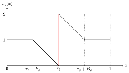
Figure 5: Distribution of the reweighting coefficient $w_{g}(x)$ for the setting of Covariate shift via Strategic Response.

Appendix D A Geometric Interpretation

In this extension of Section 4.2, we fulfill the promise of Section 3.3 and consider a case in which shared structure of between $\Psi\colon\mathds{O}^{2}\to\mathbf{R}$ and each $D_{g}\colon\mathds{G}^{2}\to\mathbf{R}$ permits a geometric interpretation of distribution shift for Equal Opportunity EOp, building on Theorem 4.3. We continue to defer rigorous proof to Appendix F.

We first recall the definition of the true positive rate of policy $\pi$, for each group, on distribution $\mathcal{T}$.

$$\beta^{+}_{g}\coloneqq\Pr_{\pi,{\mathcal{T}}}(\hat{Y}{=}1\mid Y{=}1,G{=}g)$$ (29)

The true positive rate may be expressed as a ratio of inner products defined over the space of square-integrable $L^{2}$ functions on $\mathcal{X}$.

$$\beta^{+}_{g}[{\mathcal{T}}] =\frac{\Pr_{{\mathcal{T}}}(\hat{Y}{=}1,Y{=}1\mid G{=}g)}{\Pr_{{\mathcal{T}}}(Y{=}1\mid G{=}g)}=\frac{\big{\langle}\mathsf{r}_{g}[{\mathcal{T}}],\mathsf{t}_{g}\big{\rangle}_{g}}{\big{\langle}\mathsf{r}_{g}[{\mathcal{T}}],\mathsf{1}\big{\rangle}_{g}}$$ (30)

$$\langle a,b\rangle_{g} \coloneqq\int_{\mathcal{X}}a(x)b(x)\mathsf{s}_{g}(x)\differential{x}$$ (31)

where we use the shorthands

$$\mathsf{r}_{g}[{\mathcal{T}}](x) \coloneqq\Pr_{{\mathcal{T}}}(X{=}x\mid G{=}g)$$ (32)

$$\mathsf{s}_{g}(x) \coloneqq\Pr_{{\mathcal{S}}}(Y{=}1\mid X{=}x,G{=}g)$$ (33)

$$\mathsf{1}(x) \coloneqq 1$$ (34)

$$\mathsf{t}_{g}(x) \coloneqq\Pr_{\pi}(\hat{Y}{=}1\mid Y{=}1,X=x,G=g)$$ (35)

and assume that $\mathsf{s}_{g}(x)>0$ for all $x$ and $g$.

We observe that the only degree of freedom in $\beta^{+}_{g}$ as $\mathcal{{\mathcal{T}}}$ varies subject to covariate shift is $\mathsf{r}_{g}$: by the covariate assumption, $\mathsf{s}_{g}$ is fixed; $\mathsf{t}$ meanwhile remains independent of ${\mathcal{T}}$ for fixed policy $\pi$, since $\pi$ is independent of $Y$ conditioned on $X$ and $G$.

Selection of $\mathbf{D}$

We now select each $D_{g}$ to be the standard metric for the inner product defined by Equation 31, where, for each group, distributions in $\mathds{G}$ are mapped to the corresponding vector $\mathsf{r}_{g}$:

$$D_{g}\big{(}\Pr_{{\mathcal{T}}}(X,Y\mid G{=}g)\parallel\Pr_{{\mathcal{S}}}(X,Y\mid G{=}g)\big{)}$$ (36)

$$\qquad\qquad\qquad\coloneqq\sqrt{\langle\mathsf{r}_{g}[{\mathcal{S}}],\mathsf{r}_{g}[{\mathcal{T}}]\rangle_{g}+\langle\mathsf{r}_{g}[{\mathcal{T}}],\mathsf{r}_{g}[{\mathcal{T}}]\rangle_{g}-2\langle\mathsf{r}_{g}[{\mathcal{S}}],\mathsf{r}_{g}[{\mathcal{T}}]\rangle_{g}}$$

In this geometric picture, $\mathbf{D}({\mathcal{T}}\parallel{\mathcal{S}})\preceq\mathbf{B}$ implies that all possible values for $\mathsf{r}_{g}[{\mathcal{T}}]$ lie within a ball of radius $B_{g}$ centered at $\mathsf{r}_{g}[{\mathcal{S}}]$. By the normalization condition of a probablity (density) function, denoting $\mathsf{s}_{g}^{-1}(x)\coloneqq(\mathsf{s}_{g}(x))^{-1}$, the vector $\mathsf{r}_{g}[{\mathcal{T}}]$ must also lie on the hyperplane

$$\int_{\mathcal{X}}\mathsf{r}_{g}[{\mathcal{T}}]\differential{x}=\langle\mathsf{r}_{g}[{\mathcal{T}}],\mathsf{s}_{g}^{-1}\rangle_{g}=1$$ (37)

Recalling Equation 30, the group-specific true positive rate $\beta^{+}_{g}[{\mathcal{T}}]$ for policy $\pi$ is given by a ratio of the projected distances of $\mathsf{r}_{g}$ along the $\mathsf{t}_{g}$ and $\mathsf{1}$ vectors. Let us therefore denote the projection of $\mathsf{r}_{g}[{\mathcal{T}}]$ onto the $(\mathsf{1},\mathsf{t}_{g})$-plane as $\mathsf{r}_{g}^{\perp}[{\mathcal{T}}]$. We may then consider the possible values of $\mathsf{r}_{g}^{\perp}[{\mathcal{T}}]$ as projections from the intersection of the $\mathsf{r}_{g}[{\mathcal{S}}]$-centered hypersphere of radius $B_{g}$ and the hyperplane of normalized distributions (Equation 37). Using $\angle(\cdot,\cdot)$ to denote the angle between vectors and denoting $\phi^{\prime}_{g}\coloneqq\angle(\mathsf{r}_{g},\mathsf{t}_{g})$, $\theta^{\prime}_{g}\coloneqq\angle(\mathsf{r}_{g},\mathsf{1})$, $\phi_{g}\coloneqq\angle(\mathsf{r}_{g}^{\perp},\mathsf{t}_{g})$, and $\theta_{g}\coloneqq\angle(\mathsf{r}_{g}^{\perp},\mathsf{1})$, we appeal to the geometric relationship $\langle a,b\rangle=\cos(\angle(a,b))\|a\|\|b\|$ to write

$$\beta^{+}_{g}\frac{\|\mathsf{1}\|}{\|\mathsf{t}_{g}\|}=\frac{\cos{\phi^{\prime}_{g}}}{\cos{\theta^{\prime}_{g}}}=\frac{\cos{\phi_{g}}}{\cos{\theta_{g}}}$$ (38)

From these observations, we need only bound the ratio between $\cos(\phi_{g})$ and $\cos(\theta_{g})$ to bound $\beta^{+}_{g}$. Relating these angles in the $(\mathsf{1},\mathsf{t}_{g})$-plane by $\phi_{g}=\xi_{g}-\theta_{g}$ where $\xi_{g}\coloneqq\angle(\mathsf{t}_{g},\mathsf{1})$, we arrive at the following theorem:

Theorem D.1.

The true positive rate $\beta^{+}_{g}$ is bounded over the domain of covariate shift $\mathds{D}_{\text{cov}}[\mathbf{B}]$, which we define by the bound $\mathbf{D}({\mathcal{T}}\parallel{\mathcal{S}})\preceq\mathbf{B}$, and the invariance of $\Pr(Y{=}1\mid X{=}x,G{=}g)$ for all $x,g$, as

$$\frac{\cos(\phi_{g}^{u})}{\cos(\xi_{g}-\phi_{g}^{u})}\leq\frac{\|\mathsf{1}\|}{\|\mathsf{t}_{g}\|}\beta^{+}_{g}(\pi,{\mathcal{T}})\leq\frac{\cos(\phi_{g}^{l})}{\cos(\xi_{g}-\phi_{g}^{l})}$$ (39)

with upper ($\phi_{g}^{u}$) and lower ($\phi_{g}^{l}$) bounds for $\phi_{g}$ represented as

$$\phi_{g}^{l}\coloneqq\min_{{\mathcal{T}}\in\mathds{D}_{\text{cov}}[\mathbf{B}]}\phi_{g};\quad\phi_{g}^{u}\coloneqq\max_{{\mathcal{T}}\in\mathds{D}_{\text{cov}}[\mathbf{B}]}\phi_{g}$$ (40)

We obtain a final bound on ${\Delta^{\star}}_{{\textsf{EOp}}}$ by substituting Equation 39 into Equation 17. We visualize the geometric bound on $\beta^{+}_{g}$ (Theorem D.1) in Figure 6. In Section E.1, we apply this bound to real-world credit score data assuming the model of strategic manipulation given in Section 6.1. Although the result is not an easily interpretted formula, it provides a demonstration of geometric reasoning applied to statistical fairness guarantees.

Finally, we note that, in addition to the constraints considered above, each vector $\mathsf{r}_{g}$ is subject to the positivity condition, $\forall x\in\mathcal{X},\mathsf{r}_{g}(x)\geq 0$. The bound developed in this section, however, does not benefit from this additional constraint; we leave this to potential future work.

Figure 6: A geometric bound in an infinite-dimensional vector space (i.e., a Hilbert space), represented with a stereoscopic (cross-eye) view in three dimensions (to provide intuition) and an examination of the $(\mathsf{t}_{g},\mathsf{1})$-plane. The extreme values of $\beta^{+}_{g}$ correspond to the extremal angles of $\phi$ and $\theta$. In this figure, the vector displayed parallel to $\mathsf{s}_{g}^{-1}$ from the origin terminates on the hyperplane of normalized distributions.

Appendix E Empirical Evaluations of the Bounds

E.1 Comparisons to Dynamic Models of Distribution Shift

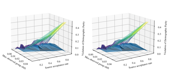
Figure 7: A stereoscopic (cross-eye view) comparison between the bound of Section 4.1 (gradated) and simulated results for the model of Section 6.1 (blue) in response to a DP-fair classifier with different initial group-independent acceptance rates. The $x$-axis represents the maximum shift $D_{g}$ over all groups $g$ in response to the classifier.

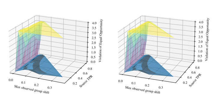
Figure 8: A stereoscopic (cross-eye view) comparison between the theoretical bound of Section 4.2 (gradated) and simulated results for the model of Section 6.1 (blue) in response to a EOp-fair classifier with different initial group-independent true positive rates (TPR). The $x$-axis represents the maximum shift $D_{g}$ over all groups $g$ in response to the classifier. As Corollary 4.4 limits the maximum possible value of EO violation, we include this limit as part of the bound.

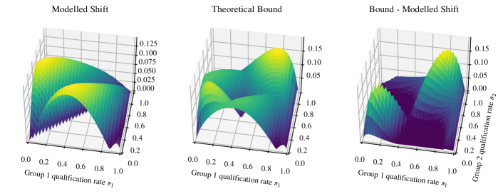
Figure 9: A policy satisfying DP is subject to distribution shift prescribed by replicator dynamics (Section 6.2). Realized disparity increases (blue) are compared to the theoretical bound (Theorem 5.2, gradated), which is tight when group have dissimilar qualification rates.

E.2 Comparisons to Real-World Data

We provide additional graphics comparing bounds on demographic parity or equal opportunity to real-world distribution shifts. Figure 10 compares the covariate shift bound of Theorem 4.1 to the violation of demographic parity for hypothetical policies trained on one US state and deployed in another. Figure 11 compares the label shift bound of Theorem 5.2 to the violation of demographic parity for hypothetical policies trained for a US state in 2014 and deployed in 2018. Figure 12 compares the covariate shift bound of Theorem 4.3 with Theorem D.1 to the violation of equal opportunity for hypothetical policies trained on one US state and deployed in another.

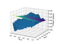
(a) CA $\longrightarrow$ AZ

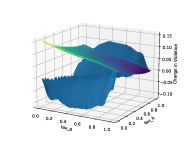
(b) CA $\longrightarrow$ CO

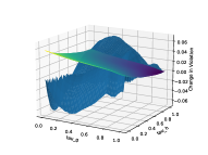
(c) CA $\longrightarrow$ FL

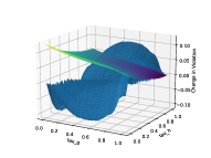
(d) CA $\longrightarrow$ MD

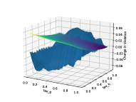
(e) CA $\longrightarrow$ OR

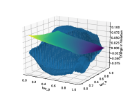
(f) CA $\longrightarrow$ UT

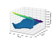
(g) CA $\longrightarrow$ VT

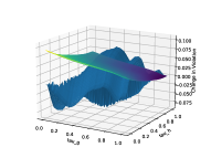
(h) CA $\longrightarrow$ WI

Figure 10: Change in violation of demographic parity for hypothetical policies trained on one US state’s data and reused for another state (blue) compared to covariate-shift bounds (Theorem 4.1, gradated). The $x$-axis and $y$-axis represent the thresholds $\tau_{g}$ and $\tau_{h}$, respectively.

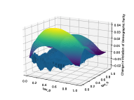
(a) Arizona (AZ)

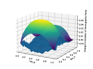
(b) Colorado (CO)

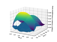
(c) Florida (FL)

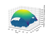
(d) Maryland (MD)

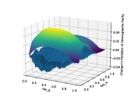
(e) Oregon (OR)

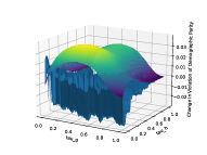
(f) Utah (UT)

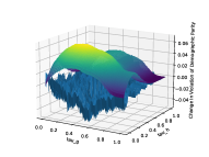
(g) Vermont (VT)

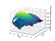
(h) Wisconsin (WI)

Figure 11: Change in violation of demographic parity for hypothetical policies trained on 2014 data and reused for 2018 (blue) compared to label-shift bounds (Theorem 5.2, gradated). The $x$-axis and $y$-axis represent the thresholds $\tau_{g}$ and $\tau_{h}$, respectively.

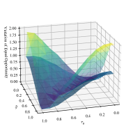
(a) CA $\longrightarrow$ NV

(b) CA $\longrightarrow$ IL

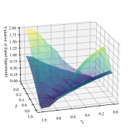
(c) NV $\longrightarrow$ IL

Figure 12: Change in violation of equal opportunity for hypothetical policies trained on one US state’s data and reused for another state (blue) compared to covariate-shift bounds (Theorems 4.3, LABEL: and D.1, gradated). The $x$-axis and $y$-axis represent the thresholds $\tau_{g}$ and $\tau_{h}$, respectively.

Appendix F Omitted Proofs

Proof of Lemma 2.7:

Statement: For all $\pi$, ${\Delta^{\star}}$, and $\mathbf{D}$, when $\mathbf{B}=0$, ${\Delta^{\star}}(\pi,{\mathcal{S}})={\Delta^{\star}}(\pi,{\mathcal{T}})$.

Proof.

By the definitions of group-vectorized shift (Definition 2.5) and divergence (Definition 2.4) together with the bounded distribution shift assumption (2.6), we note

$$\mathbf{B}=0\implies\mathbf{D}({\mathcal{T}}\parallel{\mathcal{S}})=0$$ (41)

and

$$D_{g}({\mathcal{T}}\parallel{\mathcal{S}})=0\implies\Pr_{{\mathcal{S}}}(X,Y\mid G{=}g)=\Pr_{{\mathcal{T}}}(X,Y\mid G{=}g)$$ (42)

Combining these implications and invoking the independence of $\hat{Y}\sim\pi$ and $Y$ conditioned on $X$ and $G$ (Equation 1), it follows that

$$\mathbf{B}=0\implies\forall g,\quad\Pr_{\pi,{\mathcal{S}}}(X,Y,\hat{Y}\mid G{=}g)=\Pr_{\pi,{\mathcal{T}}}(X,Y,\hat{Y}\mid G{=}g)$$ (43)

Consulting the definition of disparity (Definition 2.2), it follows that ${\Delta^{\star}}(\pi,{\mathcal{S}})$ and ${\Delta^{\star}}(\pi,{\mathcal{T}})$ are equal when $\mathbf{B}=0$. ∎

Proof of Theorem 3.2:

Statement: If there exists an $\mathbf{L}$ such that $\nabla_{\mathbf{b}}v({\Delta^{\star}},\mathbf{D},\pi,{\mathcal{S}},\mathbf{b})\preceq\mathbf{L}$, everywhere along some curve from $0$ to $\mathbf{B}$, then

$${\Delta^{\star}}(\pi,{\mathcal{T}})\leq{\Delta^{\star}}(\pi,{\mathcal{S}})+\mathbf{L}\cdot\mathbf{B}$$ (44)

Proof.

We reiterate that $v({\Delta^{\star}},\mathbf{D},\pi,{\mathcal{S}},\mathbf{b})$ defines a scalar field over the non-negative cone $\mathbf{b}\in(\mathbf{R}_{+}\cup 0)^{|\mathcal{G}|}$. Treating $v$ as a scalar potential, we may define the conservative vector field $\mathbf{F}$:

$$\mathbf{F}=\nabla_{\mathbf{b}}v$$ (45)

This formulation, in terms of a potential, ensures the path-independence of the line integral of $\mathbf{F}$ along any continuous curve $C$ from $0$ to $\mathbf{B}$. That is,

$$v(...,\mathbf{B})-v(...,0)=\int_{C}\mathbf{F}(\mathbf{b})\cdot\differential{\mathbf{b}}$$ (46)

Therefore, given a Lipshitz condition for $\mathbf{F}$ along any curve $C$ with endpoints $0$ and $\mathbf{B}$, i.e. when there exists some finite $\mathbf{L}$ such that

$$\forall\mathbf{b}\in C,\quad\mathbf{F}(\mathbf{b})\preceq\mathbf{L}$$ (47)

and therefore

$$v({\Delta^{\star}},\mathbf{D},\pi,{\mathcal{S}},\mathbf{B}) =v(...,0)+\int_{C}\mathbf{F}(\mathbf{b})\cdot\differential{\mathbf{b}}$$ (48)

$$\leq{\Delta^{\star}}(\pi,{\mathcal{S}})+\mathbf{L}\cdot\mathbf{B}$$ (49)

By the bounded distribution shift assumption (2.6), Lemma 2.7, and the definition of the supremum bound (Definition 3.1), we conclude

$${\Delta^{\star}}(\pi,{\mathcal{T}})\leq{\Delta^{\star}}(\pi,{\mathcal{S}})+\mathbf{L}\cdot\mathbf{B}$$ (50)

∎

Proof of Theorem 3.4:

Statement: Suppose, in the region $\mathbf{D}({\mathcal{T}}\parallel{\mathcal{S}})\preceq\mathbf{B}$, that $w$ is subadditive in its last argument. That is, $w(...,\mathbf{a})+w(...,\mathbf{c})\geq w(...,\mathbf{a}+\mathbf{c})$ for $\mathbf{a},\mathbf{c}\succeq 0$ and $\mathbf{a}+\mathbf{c}\preceq\mathbf{B}$. Then, a local, first-order approximation of $w(...,\mathbf{b})$ evaluated at $0$, i.e.,

$$\mathbf{L}=\nabla_{\mathbf{b}}w(...,\mathbf{b})\big{|}_{\mathbf{b}=0}=\nabla_{\mathbf{b}}v(...,\mathbf{b})\big{|}_{\mathbf{b}=0}$$ (51)

provides an upper bound for $v(...,\mathbf{B})$:

$$v({\Delta^{\star}},\mathbf{D},\pi,{\mathcal{S}},\mathbf{B})\leq{\Delta^{\star}}(\pi,{\mathcal{S}})+\mathbf{L}\cdot\mathbf{B}$$ (52)

Proof.

Represent

$$\mathbf{B}=\sum_{g}\mathbf{e}_{g}B_{g}$$ (53)

Then, invoking the definition of the derivative as a Weierstrass limit from elementary calculus, as well as Lemma 2.7, and by repeatedly appealing to the assumed subadditivity condition within our domain, we find

$$\mathbf{B}\cdot\mathbf{L} =\mathbf{B}\cdot\nabla_{\mathbf{b}}v(\pi,{\mathcal{S}},\mathbf{b})\big{|}_{\mathbf{b}=0}$$ (54a)

$$=\sum_{g}B_{g}\frac{d}{dx}v(\pi,{\mathcal{S}},x\mathbf{e}_{g})\big{|}_{x=0}$$ (54b)

$$=\sum_{g}B_{g}\lim_{N\to\infty}N\Big{(}v(\pi,{\mathcal{S}},\frac{1}{N}\mathbf{e}_{g})-v(\pi,{\mathcal{S}},0)\Big{)}$$ (54c)

$$=\sum_{g}B_{g}\lim_{N\to\infty}N\Big{(}w(\pi,{\mathcal{S}},\frac{1}{N}\mathbf{e}_{g})\Big{)}$$ (54d)

$$\geq\sum_{g}B_{g}\leavevmode\nobreak\ w(\pi,{\mathcal{S}},\mathbf{e}_{g})$$ (54e)

$$\geq\sum_{g}w(\pi,{\mathcal{S}},B_{g}\mathbf{e}_{g})$$ (54f)

$$\geq w(\pi,{\mathcal{S}},\mathbf{B})$$ (54g)

Also recall (Definition 3.3)

$$w(\pi,{\mathcal{S}},\mathbf{B}) \coloneqq v(\pi,{\mathcal{S}},\mathbf{B})-{\Delta^{\star}}(\pi,{\mathcal{S}})$$ (55)

Therefore, we obtain

$$v(\pi,{\mathcal{S}},\mathbf{B})\leq{\Delta^{\star}}(\pi,{\mathcal{S}})+\mathbf{B}\cdot\mathbf{L}$$ (56)

∎

Lemma F.1.

For each group $g\in\mathcal{G}$, under covariate shift,

$$\Pr_{\pi,{\mathcal{T}}} \Big{(}\hat{Y}{=}1\mid G{=}g\Big{)}-\Pr_{\pi,{\mathcal{S}}}\Big{(}\hat{Y}{=}1\mid G{=}g\Big{)}=\operatorname*{Cov}_{\pi,{\mathcal{S}}}\Big{[}\omega_{g}({\mathcal{T}},{\mathcal{S}},X),\Pr_{\pi(X,g)}(\hat{Y}{=}1)\Big{]}$$ (57)

Proof.

First, note that $\operatorname*{\mathbb{E}}_{{\mathcal{S}}}[\omega_{g}({\mathcal{T}},{\mathcal{S}},x)]=1$, since

$$\operatorname*{\mathbb{E}}_{{\mathcal{S}}}[\omega_{g}({\mathcal{T}},{\mathcal{S}},x)] =\int_{\mathcal{X}}\omega_{g}({\mathcal{T}},{\mathcal{S}},x)\Pr_{{\mathcal{S}}}(X=x\mid G{=}g)\differential{x}$$

$$=\int_{\mathcal{X}}\frac{\Pr_{{\mathcal{T}}}(X{=}x\mid G{=}g)}{\Pr_{{\mathcal{S}}}(X{=}x\mid G=g)}\Pr_{{\mathcal{S}}}(X{=}x\mid G{=}g)\differential{x}$$

$$=\int_{\mathcal{X}}{\Pr_{{\mathcal{T}}}(X{=}x\mid G{=}g)}\differential{x}=1$$

Then, adopting the shorthand $\omega_{g}(x)=\omega_{g}({\mathcal{T}},{\mathcal{S}},x)$, we have:

$$\Pr_{\pi,{\mathcal{T}}}\Big{(}\hat{Y}{=}1\mid G{=}g\Big{)}-\Pr_{\pi,{\mathcal{S}}}\Big{(}\hat{Y}{=}1\mid G{=}g\Big{)}$$ (58)

$$= \int_{\mathcal{X}}\Pr_{\pi(x,g)}(\hat{Y}{=}1)\Pr_{{\mathcal{T}}}(X{=}x\mid G{=}g)\differential{x}-\int_{\mathcal{X}}\Pr_{\pi(x,g)}(\hat{Y}{=}1)\Pr_{{\mathcal{S}}}(X{=}x\mid G{=}g)\differential{x}$$ (59)

$$= \int_{\mathcal{X}}\Pr_{\pi(x,g)}(\hat{Y}{=}1)\Big{(}\omega_{g}(x)-1\Big{)}\Pr_{{\mathcal{S}}}(X{=}x\mid G{=}g)\differential{x}$$ (60)

$$= \ \operatorname*{\mathbb{E}}_{{\mathcal{S}}}\Big{[}\Pr_{\pi(x,g)}(\hat{Y}{=}1)(\omega_{g}(x)-1)\mid G{=}g\Big{]}$$ (61)

$$= \ \operatorname*{\mathbb{E}}_{{\mathcal{S}}}\Big{[}\Pr_{\pi(x,g)}(\hat{Y}{=}1)(\omega_{g}(x)-\operatorname*{\mathbb{E}}_{{\mathcal{S}}}[\omega_{g}(x)])\mid G{=}g\Big{]} \operatorname*{\mathbb{E}}_{{\mathcal{S}}}[\omega_{g}(x)]=1$$ (since )

$$= \ \operatorname*{\mathbb{E}}_{{\mathcal{S}}}\Big{[}(\Pr_{\pi(x,g)}(\hat{Y}{=}1)-\operatorname*{\mathbb{E}}_{{\mathcal{S}}}[\Pr_{\pi(x,g)}(\hat{Y}{=}1)](\omega_{g}(x)-\operatorname*{\mathbb{E}}_{{\mathcal{S}}}[\omega_{g}(x)])\mid G{=}g\Big{]} \operatorname*{\mathbb{E}}[f(x)-\operatorname*{\mathbb{E}}[f(x)]]=0$$ ()

$$= \ \operatorname*{Cov}_{\pi,{\mathcal{S}}}\Big{[}w_{g}({\mathcal{T}},{\mathcal{S}},X),\Pr_{\pi(x,g)}(\hat{Y}{=}1)\Big{]}$$ (62)

∎

Lemma F.2.

If $X$ is a random variable and $X\in[0,1]$, then $\operatorname*{Var}(X)\leq\operatorname*{\mathbb{E}}[X](1-\operatorname*{\mathbb{E}}(X))$.

Proof.

$$\operatorname*{Var}[X] =\operatorname*{\mathbb{E}}[(X-\operatorname*{\mathbb{E}}[X])^{2}]$$

$$=\operatorname*{\mathbb{E}}[X^{2}]-(\operatorname*{\mathbb{E}}[X])^{2}$$

$$\leq\operatorname*{\mathbb{E}}[X]-(\operatorname*{\mathbb{E}}[X])^{2} X\in[0,1]$$ ()

$$=\operatorname*{\mathbb{E}}[X](1-\operatorname*{\mathbb{E}}(X))$$

∎

Proof of Theorem 4.1:

Statement: For demographic parity between two groups under covariate shift (denoting, for each $g$, $\beta_{g}\coloneqq\Pr_{\pi,{\mathcal{S}}}(\hat{Y}{=}1\mid G{=}g)$),

$${\Delta^{\star}}_{{\textsf{DP}}}(\pi,{\mathcal{T}})\leq{\Delta^{\star}}_{{\textsf{DP}}}(\pi,{\mathcal{S}})+\sum_{g}\Big{(}\beta_{g}(1-\beta_{g})B_{g}\Big{)}^{\nicefrac{{1}}{{2}}}$$ (63)

Proof.

Again adopting the shorthand $\omega_{g}(x)=\omega_{g}({\mathcal{T}},{\mathcal{S}},x)$,

$${\Delta^{\star}}(\pi,{\mathcal{T}})$$ (64)

$$=\Big{|}\Pr_{\pi,{\mathcal{T}}}\Big{(}\hat{Y}{=}1\mid G{=}g\Big{)}-\Pr_{\pi,{\mathcal{T}}}\Big{(}\hat{Y}{=}1\mid G{=}h\Big{)}\Big{|}$$ (65)

$$=\Big{|}\Pr_{\pi,{\mathcal{T}}}\Big{(}\hat{Y}{=}1\mid G{=}g\Big{)}-\Pr_{\pi,{\mathcal{S}}}\Big{(}\hat{Y}{=}1\mid G{=}g\Big{)}$$ (66)

$$\qquad+\Pr_{\pi,{\mathcal{S}}}\Big{(}\hat{Y}{=}1\mid G{=}g\Big{)}-\Pr_{\pi,{\mathcal{S}}}\Big{(}\hat{Y}{=}1\mid G{=}h\Big{)}$$ (67)

$$\qquad+\Pr_{\pi,{\mathcal{S}}}\Big{(}\hat{Y}{=}1\mid G{=}h\Big{)}-\Pr_{\pi,{\mathcal{T}}}\Big{(}\hat{Y}{=}1\mid G{=}h\Big{)}\Big{|}$$ (68)

$$\leq{\Delta^{\star}}(\pi,{\mathcal{S}})+\operatorname*{Cov}_{{\mathcal{S}}}\Big{[}\omega_{g}(x),\Pr_{\pi(x,g)}(\hat{Y}{=}1)\Big{]}+\operatorname*{Cov}_{{\mathcal{S}}}\Big{[}\omega_{h}(x),\Pr_{\pi(x,h)}(\hat{Y}{=}1)\Big{]}$$ (By Lemma F.1)

$$\leq{\Delta^{\star}}(\pi,{\mathcal{S}})+\sqrt{\operatorname*{Var}_{{\mathcal{S}}}[\omega_{g}(x)]}\cdot\sqrt{\operatorname*{Var}_{{\mathcal{S}}}[\Pr_{\pi(x,g)}(\hat{Y}{=}1)]}+\sqrt{\operatorname*{Var}_{{\mathcal{S}}}[\omega_{h}]}\cdot\sqrt{\operatorname*{Var}_{{\mathcal{S}}}[\Pr_{\pi(x,h)}(\hat{Y}{=}1)]} \big{|}\operatorname*{Cov}[a,b]\big{|}\leq\sqrt{\operatorname*{Var}[a]}\cdot\sqrt{\operatorname*{Var}[b]}$$ ()

$$\leq{\Delta^{\star}}(\pi,{\mathcal{S}})+\sqrt{\operatorname*{Var}_{{\mathcal{S}}}[\omega_{g}(x)]}\cdot\sqrt{\operatorname*{\mathbb{E}}_{{\mathcal{S}}}[\Pr_{\pi(x,g)}(\hat{Y}{=}1)](1-\operatorname*{\mathbb{E}}_{{\mathcal{S}}}[\Pr_{\pi(x,g)}(\hat{Y}{=}1)])}$$ (69)

$$\qquad\qquad\quad+\sqrt{\operatorname*{Var}_{{\mathcal{S}}}(\omega_{h}(x))}\cdot\sqrt{\operatorname*{\mathbb{E}}_{{\mathcal{S}}}[\Pr_{\pi(x,h)}(\hat{Y}{=}1)](1-\operatorname*{\mathbb{E}}_{{\mathcal{S}}}[\Pr_{\pi(x,h)}(\hat{Y}{=}1))]} \hat{Y}\in\{0,1\}$$ (, and Lemma F.2)

$$={\Delta^{\star}}(\pi,{\mathcal{S}})+\sqrt{\operatorname*{Var}_{{\mathcal{S}}}[\omega_{g}(x)]}\cdot\sqrt{\beta_{g}(1-\beta_{g})}+\sqrt{\operatorname*{Var}_{{\mathcal{S}}}[\omega_{h}(x)]}\cdot\sqrt{\beta_{h}(1-\beta_{h})} \beta_{g}=\Pr_{\pi,{\mathcal{S}}}(\hat{Y}{=}1|G{=}g)=\operatorname*{\mathbb{E}}_{{\mathcal{S}}}[\mathbbm{1}_{\pi(x,g)}(\hat{Y}{=}1)]$$ ()

$$={\Delta^{\star}}(\pi,{\mathcal{S}})+\sum_{g}\Big{(}\beta_{g}(1-\beta_{g})\operatorname*{Var}_{{\mathcal{S}}}[\omega_{g}({\mathcal{T}},{\mathcal{S}},x)]\Big{)}^{\nicefrac{{1}}{{2}}}$$ (70)

∎

Proof of Corollary 4.2: Statement: Theorem 4.1 Theorem 4.1 may be generalized to multiple classes $\mathcal{Y}=\{1,2,...,m\}$ and multiple groups $\mathcal{G}\in\{1,2,...,n\}$,

$${\Delta^{\star}_{{\textsf{DP}}}}(\pi,{\mathcal{T}})\coloneqq\sum_{y\in\mathcal{Y}}\sum_{g,h\in\mathcal{G}}\Big{|}\Pr_{\pi,{\mathcal{T}}}(\hat{Y}{=}y\mid G{=}g)-\Pr_{\pi,{\mathcal{T}}}(\hat{Y}{=}y\mid G{=}h)\Big{|}$$ (71)

$${\Delta^{\star}}_{{\textsf{DP}}}(\pi,{\mathcal{T}})\leq{\Delta^{\star}}_{{\textsf{DP}}}(\pi,{\mathcal{S}})+\sum_{y\in\mathcal{Y}}\sum_{g,h\in\mathcal{G}}\big{(}\beta_{g,y}(1-\beta_{g,y})B_{g}\big{)}^{\nicefrac{{1}}{{2}}}$$ (72)

where $\beta_{g,y}=\Pr(\hat{Y}{=}y\mid G{=}g)$, and assuming $\operatorname*{Var}_{{\mathcal{S}}}[w_{g}({\mathcal{S}},{\mathcal{T}},X)]\leq B_{g}$.

Proof.

We again adopt the shorthand $\omega_{g}(x)=\omega_{g}({\mathcal{T}},{\mathcal{S}},x)$. We first generalize Lemma F.1. For each group $g\in\mathcal{G}$, under covariate shift, for all $y\in\mathcal{Y}$,

$$\Pr_{\pi,{\mathcal{T}}} \Big{(}\hat{Y}{=}y\mid G{=}g\Big{)}-\Pr_{\pi,{\mathcal{S}}}\Big{(}\hat{Y}{=}y\mid G{=}g\Big{)}=\operatorname*{Cov}_{\pi,{\mathcal{S}}}\Big{[}\omega_{g}({\mathcal{S}},{\mathcal{T}},X),\Pr_{\pi(X,g)}(\hat{Y}{=}y)\Big{]}$$ (73)

Retracing the logic of Theorem 4.1, for $\operatorname*{Var}_{{\mathcal{S}}}[\omega_{g}({\mathcal{T}},{\mathcal{S}},x)]\leq B_{g}$, it follows that

$${\Delta^{\star}_{{\textsf{DP}}}}(\pi,{\mathcal{T}}) \coloneqq\sum_{y\in\mathcal{Y}}\sum_{g,h\in\mathcal{G}}\Big{|}\Pr_{\pi,{\mathcal{T}}}(\hat{Y}{=}y\mid G{=}g)-\Pr_{\pi,{\mathcal{T}}}(\hat{Y}{=}y\mid G{=}h)\Big{|}$$ (74)

$$\leq{\Delta^{\star}_{{\textsf{DP}}}}(\pi,{\mathcal{S}})+\sum_{y\in\mathcal{Y}}\sum_{g,h\in\mathcal{G}}\sqrt{\big{(}\beta_{g,y}(1-\beta_{g,y})\operatorname*{Var}_{{\mathcal{S}}}[\omega_{g}(x)]\big{)}}$$ (75)

$$\leq{\Delta^{\star}_{{\textsf{DP}}}}(\pi,{\mathcal{S}})+\sum_{y\in\mathcal{Y}}\sum_{g,h\in\mathcal{G}}\sqrt{\big{(}\beta_{g,y}(1-\beta_{g,y})B_{g}\big{)}}$$ (76)

$$={\Delta^{\star}_{{\textsf{DP}}}}(\pi,{\mathcal{S}})+\sum_{y\in\mathcal{Y}}\sum_{g,h\in\mathcal{G}}\big{(}\beta_{g,y}(1-\beta_{g,y})B_{g}\big{)}^{\nicefrac{{1}}{{2}}}$$ (77)

∎

Proof of Theorem 4.3

Statement: Subject to covariate shift and any given $\mathbf{D},\mathbf{B}$, assume extremal values for $\beta_{g}^{+}$, i.e.,

$$\forall g,\leavevmode\nobreak\ \leavevmode\nobreak\ D_{g}({\mathcal{T}}\parallel{\mathcal{S}})<B_{g}\implies l_{g}\leq\beta^{+}_{g}(\pi,{\mathcal{T}})<u_{g}$$ (78)

then, for $v$ corresponding to ${\Delta^{\star}}_{{\textsf{EOp}}}$,

$$v({\Delta^{\star}}_{{\textsf{EOp}}},\mathbf{D},\pi,{\mathcal{S}},\mathbf{B})\leq\max_{x_{g}\in\{l_{g},u_{g}\}}\sum_{g,h}\Big{|}x_{g}-x_{h}\Big{|}$$ (79)

Proof.

Recall that, for this setting,

$$v({\Delta^{\star}}_{{\textsf{EOp}}},\mathbf{D},\pi,{\mathcal{S}},\mathbf{B})=\sup_{\mathbf{D}({\mathcal{T}}\parallel{\mathcal{S}})\preceq\mathbf{B}}{\Delta^{\star}}_{{\textsf{EOp}}}$$ (80)

and

$${\Delta^{\star}}_{{\textsf{EOp}}}=\sum_{g,h}|\beta_{g}^{+}-\beta_{h}^{+}|$$ (81)

This latter expression is convex in each $\beta_{g}^{+}$. Therefore, ${\Delta^{\star}}_{{\textsf{EOp}}}$ is maximized on the boundary of its domain, i.e. $\beta^{+}_{g}\in\{l_{g},u_{g}\}$ for each $g$, given the assumption of the theorem. ∎

Proof of Corollary 4.4

Statement: The disparity measurement ${\Delta^{\star}}_{\textsf{EOp}}$ cannot exceed $\frac{|\mathcal{G}|^{2}}{4}$.

Proof.

We note that each $\beta^{+}_{g}$ is ultimately confined to the interval $[0,1]$. Building on our proof for Theorem 4.3, to maximize ${\Delta^{\star}}_{{\textsf{EOp}}}$, we must consider the boundary of this domain, where, for each $g$, $\beta^{+}_{g}\in\{0,1\}$. Because the only terms that contribute to ${\Delta^{\star}}_{{\textsf{EOp}}}$ are those in which $\beta_{g}^{+}=1$ and $\beta_{h}^{+}=0$ (as opposed to $\beta_{g}^{+}=\beta_{h}^{+}$), we seek to maximize the number of such terms. This occurs when as close to half of the groups as possible have one extremal true positive rate (e.g., without loss of generality, $\beta^{+}_{g}=1$) and the remaining groups have the other (e.g., $\beta^{+}_{g}=0$). In such cases, ${\Delta^{\star}}_{{\textsf{EOp}}}$ is given by

$$\max{\Delta^{\star}}_{{\textsf{EOp}}}=\lfloor\frac{\mathcal{G}}{2}\rfloor\lceil\frac{\mathcal{G}}{2}\rceil\leq\frac{|\mathcal{G}|^{2}}{4}$$ (82)

∎

Proof of Theorem 5.1:

Statement: A Lipshitz condition bounds $\nabla_{\mathbf{b}}v({\Delta^{\star}}_{\textsf{DP}},\mathbf{D},\pi,{\mathcal{S}},\mathbf{b})$ when

$$D_{g}({\mathcal{T}}\parallel{\mathcal{S}})\coloneqq\Big{|}Q_{g}(\mathcal{S})-Q_{g}(\mathcal{{\mathcal{T}}})\Big{|}\leq B_{g}$$ (83)

Specifically,

$$\partialderivative{b_{g}}v({\Delta^{\star}}_{\textsf{DP}},\mathbf{D},\pi,{\mathcal{S}},\mathbf{b})\leq(|\mathcal{G}|-1)\Big{|}\beta^{+}_{g}-\beta^{-}_{g}\Big{|}$$ (84)

for true positive rates $\beta^{+}_{g}$ and false positive rates $\beta^{-}_{g}$:

$$\beta^{+}_{g}\coloneqq\Pr_{\pi}(\hat{Y}{=}1{\mid}Y{=}1,G{=}g)\quad;\quad\beta^{-}_{g}\coloneqq\Pr_{\pi}(\hat{Y}{=}1{\mid}Y{=}0,G{=}g)$$ (85)

Proof.

We first establish that $D_{g}^{({\textsf{DP}})}({\mathcal{T}}\parallel{\mathcal{S}})=|Q_{g}({\mathcal{S}})-Q_{g}({\mathcal{T}})|$, where

$$Q_{g}({\mathcal{T}})\coloneqq\Pr_{\mathcal{T}}(Y{=}1\mid G{=}g)$$ (86)

is an appropriate measure of group-conditioned distribution shift (Definition 2.5). That $\mathbf{D}$ satisfies the axioms of a divergence on group-conditioned distributions subject to the label shift assumption ($\Pr_{\mathcal{T}}(X\mid Y,G)=\Pr_{\mathcal{S}}(X\mid Y,G)$) and unchanging group sizes is easily verified:

$$\forall{\mathcal{S}},{\mathcal{T}},\quad D_{g}({\mathcal{T}}\parallel{\mathcal{S}})=|Q_{g}({\mathcal{S}})-Q_{g}({\mathcal{T}})| \geq 0$$ (87)

$$D_{g}({\mathcal{T}}\parallel{\mathcal{S}})=|Q_{g}({\mathcal{T}})-Q_{g}({\mathcal{T}})| =0$$ (88)

and

$$\forall g,\quad D_{g}({\mathcal{T}}\parallel{\mathcal{S}})=0 \implies\Pr_{\mathcal{T}}(Y\mid G)=\Pr_{\mathcal{S}}(Y\mid G)$$ (89)

$$\implies\Pr_{\mathcal{T}}(Y,X\mid G)=\Pr_{\mathcal{S}}(Y,X\mid G)$$ (90)

We next show that $(|\mathcal{G}|-1)|\beta_{g}^{+}-\beta_{g}^{-}|$ is the corresponding Lipshitz bound for the slope of $v$ with respect to $B_{g}$, where we recall

$$\forall g,\quad\beta^{+}_{g}\coloneqq\Pr_{\pi,{\mathcal{T}}}\Big{(}\hat{Y}{=}1\mid Y{=}1,G{=}g\Big{)}$$ (91)

$$\forall g,\quad\beta^{-}_{g}\coloneqq\Pr_{\pi,{\mathcal{T}}}\Big{(}\hat{Y}{=}1\mid Y{=}{-}1,G{=}g\Big{)}$$ (92)

That is, we wish to show

$$\partialderivative{b_{g}}v({\Delta^{\star}_{{\textsf{DP}}}},\mathbf{D},\pi,{\mathcal{S}},\mathbf{b})\leq(|\mathcal{G}|-1)|\beta_{g}^{+}-\beta_{g}^{-}|$$ (93)

This follows directly from recognition that ${\Delta^{\star}_{{\textsf{DP}}}}$ is locally always affine in the acceptance rate for each group, with slope bounded by one less than the number of groups.

$${\Delta^{\star}_{{\textsf{DP}}}}=\sum_{g,h\in\mathcal{G}}|\beta_{g}-\beta_{h}|\implies\partialderivative{\beta_{g}}{\Delta^{\star}_{{\textsf{DP}}}}\leq|\mathcal{G}|-1$$ (94)

By the definition of conditional probability,

$$\beta_{g} \coloneqq\Pr(\hat{Y}{=}1)=\beta_{g}^{+}Q_{g}+\beta_{g}^{-}(1-Q_{g})$$ (95)

$$\partialderivative{Q_{g}}\beta_{g} =\beta_{g}^{+}-\beta_{g}^{-}$$ (96)

It follows by the chain rule that, for all ${\mathcal{T}}$ mutated from ${\mathcal{S}}$ subject to label shift,

$$\partialderivative{Q_{g}({\mathcal{T}})}{\Delta^{\star}_{{\textsf{DP}}}}(\pi,{\mathcal{T}})\leq(|\mathcal{G}|-1)|\beta_{g}^{+}-\beta_{g}^{-}|$$ (97)

By the linearity of derivatives, for fixed ${\mathcal{S}}$, this implies that for all ${\mathcal{T}}$ attainable via label shift,

$$\partialderivative{|Q_{g}({\mathcal{T}})-Q_{g}({\mathcal{S}})|}{\Delta^{\star}_{{\textsf{DP}}}}(\pi,{\mathcal{T}})\leq(|\mathcal{G}|-1)|\beta_{g}^{+}-\beta_{g}^{-}|$$ (98)

Since this equation holds for all ${\mathcal{T}}$, it must also hold when evaluated at $v$, the supremum of ${\Delta^{\star}}$. It follows that

$$\partialderivative{B_{g}}v({\Delta^{\star}_{{\textsf{DP}}}},\mathbf{D}^{({\textsf{DP}})},\pi,{\mathcal{S}},\mathbf{B})\leq(|\mathcal{G}|-1)|\beta_{g}^{+}-\beta_{g}^{-}|$$ (99)

∎

Proof of Theorem 5.2:

Statement: For DP under the bounded label-shift assumption $\forall g,|Q_{g}({\mathcal{S}})-Q_{g}({\mathcal{T}})|\leq B_{g}$,

$${\Delta^{\star}_{{\textsf{DP}}}}(\pi,{\mathcal{T}})\leq{\Delta^{\star}_{{\textsf{DP}}}}(\pi,{\mathcal{S}})+(|\mathcal{G}|-1)\sum_{g}B_{g}\ \Big{|}\beta^{+}_{g}-\beta^{-}_{g}\Big{|}$$ (100)

Proof.

This follows from the Lipshitz property implied by Theorem 5.1 (Equation 99) and Theorem 3.2. ∎

F.1 Omitted details for Section 6.1

Lemma F.3.

Recall the covariate shift reweighting coefficient $\omega_{g}(x)$, defined in Section 4.1.

$$\omega_{g}(x)\coloneqq\frac{\Pr_{{\mathcal{T}}}(X{=}x\mid G{=}g)}{\Pr_{{\mathcal{S}}}(X{=}x\mid G{=}g)}$$ (101)

For our assumed setting,

$$\omega_{g}(x)=\begin{cases}1,&x\in[0,\tau_{g}-{m_{g}})\\ \frac{\tau_{g}-x}{m_{g}},&x\in[\tau_{g}-{m_{g}},\tau_{g})\\ \frac{1}{m_{g}}(-x+\tau_{g}+2m_{g}),&x\in[\tau_{g},\tau_{g}+m_{g})\\ 1,&x\in[\tau_{g}+m_{g},1]\end{cases}$$ (102)

Proof for Lemma F.3:

Proof.

We discuss the target distribution by cases:

• For the target distribution between $[0,\tau_{g}-M_{g}]$: since we assume the agents are rational, under assumption 6.2, agents with feature that is smaller than $[0,\tau_{g}-M_{g}]$ will not perform any kinds of adaptations, and no other agents will adapt their features to this range of features either, so the distribution between $[0,\tau_{g}-M_{g}]$ will remain the same as before.

• For target distribution between $[\tau_{g}-M_{g},\tau_{g}]$, it can be directly calculated from assumption 6.3.

• For distribution between $[\tau_{g},\tau_{g}+M_{g}]$, consider a particular feature $x^{\star}\in[\tau_{g},\tau_{g}+M_{g}]$, under 6.4, we know its new distribution becomes:

  $$\Pr_{\mathcal{T}}(x=x^{\star}) =1+\int_{x^{\star}-M_{g}}^{\tau_{g}}\frac{1-\frac{\tau_{g}-z}{M_{g}}}{M_{g}-\tau_{g}+z}dz$$

  $$=1+\int_{x^{\star}-M_{g}}^{\tau_{g}}\frac{1}{M_{g}}dz$$

  $$=\frac{1}{M_{g}}(-x^{\star}+\tau_{g}+2M_{g})$$

• For the target distribution between $[\tau_{g}+M_{g},1]$: under assumption 6.2 and 6.4, we know that no agents will change their feature to this feature region. So the distribution between $[\tau_{g}+M_{g},1]$ remains the same as the source distribution.

Thus, the new feature distribution of $x^{(M_{g})}_{\tau_{g}}$ after agents from group $g$ strategic responding becomes:

$$\Pr_{\mathcal{T}}(x)=\Pr(x^{(M_{g})}_{\tau_{g}})=\begin{cases}1,\ \ &x\in[0,\tau_{g}-{M_{g}})\leavevmode\nobreak\ \text{and}\leavevmode\nobreak\ x\in[\tau_{g}+M_{g},1]\\ \frac{\tau_{g}-x}{M_{g}},&x\in[\tau_{g}-{M_{g}},\tau_{g})\\ \frac{1}{M_{g}}(-x+\tau_{g}+2M_{g}),&x\in[\tau_{g},\tau_{g}+M_{g})\\ 0,&\text{otherwise}\end{cases}$$ (103)

∎

Proof of Proposition 6.5:

Statement: For our assumed setting of strategic response involving DP for two groups $\{g,h\}$, Theorem 4.1 implies

$${\Delta^{\star}_{{\textsf{DP}}}}(\pi,{\mathcal{T}})\leq{\Delta^{\star}_{{\textsf{DP}}}}(\pi,{\mathcal{S}})+\tau_{g}(1-\tau_{g})\frac{2}{3}m_{g}+\tau_{h}(1-\tau_{h})\frac{2}{3}m_{h}$$ (104)

Proof.

According to Lemma F.3, we can compute the variance of $w_{g}(x)$: $\operatorname*{Var}(w_{g}(x))=\operatorname*{\mathbb{E}}\Big{[}\big{(}w_{g}(x)-\operatorname*{\mathbb{E}}[w_{g}(x)]\big{)}^{2}\Big{]}=\frac{2}{3}M_{g}$. Then by plugging it to the general bound for Theorem 4.1 gives us the result. ∎

Proof of Theorem 6.6:

Statement: For DP subject to label replicator dynamics,

$${\Delta^{\star}_{{\textsf{DP}}}}(\pi,{\mathcal{T}})\leq{\Delta^{\star}_{{\textsf{DP}}}}(\pi,{\mathcal{S}})+\sum_{g}\Big{|}Q_{g}[t+1]-Q_{g}[t]\Big{|}\frac{|\rho^{{1,1}}_{g}-\rho^{{0,1}}_{g}|}{\rho^{{1,1}}_{g}+\rho^{{0,1}}_{g}}$$ (105)

Proof.

We may directly substitute

$$|\mathcal{G}|=2$$

$$B_{g}=\Big{|}Q_{g}[t+1]-Q_{g}[t]\Big{|}$$

$$\Big{|}\beta^{+}_{g}-\beta^{-}_{g}\Big{|}=\frac{|\rho^{{1,1}}_{g}-\rho^{{0,1}}_{g}|}{\rho^{{1,1}}_{g}+\rho^{{0,1}}_{g}}$$

into Theorem 5.2. ∎

Proof of Theorem D.1:

Statement: The true positive rate $\beta^{+}_{g}$ is bounded over the domain of covariate shift $\mathds{D}_{\text{cov}}[\mathbf{B}]$, which we define by the bound $\mathbf{D}({\mathcal{T}}\parallel{\mathcal{S}})\preceq\mathbf{B}$, and the invariance of $\Pr(Y{=}1\mid X{=}x,G{=}g)$ for all $x,g$, as

$$\frac{\cos(\phi_{g}^{u})}{\cos(\xi_{g}-\phi_{g}^{u})}\leq\beta^{+}_{g}(\pi,{\mathcal{T}})\leq\frac{\cos(\phi_{g}^{l})}{\cos(\xi_{g}-\phi_{g}^{l})}$$ (106)

where

$$\phi_{g}^{l}\coloneqq\min_{{\mathcal{D}}\in\mathds{D}_{\text{cov}}[\mathbf{B}]}\phi_{g}[{\mathcal{D}}];\quad\phi_{g}^{u}\coloneqq\max_{{\mathcal{D}}\in\mathds{D}_{\text{cov}}[\mathbf{B}]}\phi_{g}[{\mathcal{D}}]$$ (107)

Proof.

To be rigorous, we may give an explicit expression for $\mathsf{r}_{g}^{\perp}$ by implicitly forming a basis in the $(\mathsf{1},\mathsf{t}_{g})$-plane via the Gram-Schmidt process.

$$\mathsf{r}_{g}^{\perp} \coloneqq\langle\mathsf{r}_{g},\mathsf{t}_{g}\rangle_{g}\frac{\mathsf{t}_{g}}{\|\mathsf{t}_{g}\|^{2}}+\langle\mathsf{r}_{g},\mathsf{u}_{g}\rangle_{g}\frac{\mathsf{u}_{g}}{\|\mathsf{u}_{g}\|^{2}}$$ (108)

$$\mathsf{u}_{g} \coloneqq\mathsf{1}-\langle\mathsf{1},\mathsf{t}_{g}\rangle\frac{\mathsf{t}_{g}}{\|\mathsf{t}_{g}\|^{2}}$$ (109)

From which we may verify that

$$\langle\mathsf{u}_{g},\mathsf{t}_{g}\rangle =0$$ (111)

$$\langle\mathsf{r}_{g}^{\perp},\mathsf{t}_{g}\rangle_{g} =\langle\mathsf{r}_{g},\mathsf{t}_{g}\rangle_{g}$$ (112)

$$\langle\mathsf{r}_{g}^{\perp},\mathsf{u}_{g}\rangle_{g} =\langle\mathsf{r}_{g},\mathsf{u}_{g}\rangle_{g}$$ (113)

$$\langle\mathsf{r}_{g}^{\perp},\mathsf{1}\rangle_{g} =\langle\mathsf{r}_{g},\mathsf{1}\rangle_{g}$$ (114)

Recalling the relationship between the cosine of an angle between two vectors and inner products:

$$\cos(\angle(a,b))=\frac{\langle a,b\rangle}{\|a\|\|b\|}$$ (115)

It follows from Equation 31 that, defining $\xi_{g}\coloneqq\angle(\mathsf{t}_{g},\mathsf{1})$,

$$\beta^{+}_{g}\frac{\|\mathsf{1}\|}{\|\mathsf{t}_{g}\|}=\frac{\cos(\angle(\mathsf{r}_{g},\mathsf{t}_{g}))}{\cos(\angle(\mathsf{r}_{g},\mathsf{1}))}=\frac{\cos(\angle(\mathsf{r}_{g}^{\perp},\mathsf{t}_{g}))}{\cos(\angle(\mathsf{r}_{g}^{\perp},\mathsf{1}))}=\frac{\cos(\phi_{g})}{\cos(\xi_{g}-\phi_{g})}$$ (116)

By the monotonicity of the final expression above with respect to $\phi_{g}$, for fixed $\xi_{g}$:

$$\derivative{x}\frac{\cos(x)}{\cos(\xi-x)}=-\frac{\sin(x)\cos(\xi-x)+\cos(x)\sin(\xi-x)}{\cos^{2}(\xi-x)}=-\frac{\sin(\xi)}{\cos^{2}(\xi-x)}$$ (117)

We note that Equation 117 is strictly negative, thus the expression in Equation 116 must be monotonic for fixed $\xi$. We may conclude that $\beta^{+}_{g}$ is extremized with extremal values of $\phi_{g}$, denoted as $\phi_{g}^{u}$ and $\phi_{g}^{l}$. ∎

References

- An et al. [2022] Bang An, Zora Che, Mucong Ding, and Furong Huang. Transferring fairness under distribution shifts via fair consistency regularization. arXiv preprint arXiv:2206.12796, 2022.
- Ben-David et al. [2010] Shai Ben-David, John Blitzer, Koby Crammer, Alex Kulesza, Fernando Pereira, and Jennifer Vaughan. A theory of learning from different domains. Machine Learning, 79:151–175, 2010.
- Biswas and Mukherjee [2021] Arpita Biswas and Suvam Mukherjee. Ensuring fairness under prior probability shifts. In Proceedings of the 2021 AAAI/ACM Conference on AI, Ethics, and Society, pages 414–424, 2021.
- Blake [1998] Catherine Blake. Uci repository of machine learning databases. 1998.
- Chen et al. [2021] Yatong Chen, Jialu Wang, and Yang Liu. Linear classifiers that encourage constructive adaptation. In Algorithmic Recourse workshop at ICML’21, 2021.
- Chouldechova [2017] Alexandra Chouldechova. Fair prediction with disparate impact: A study of bias in recidivism prediction instruments. Big data, 5(2):153–163, 2017.
- Coate and Loury [1993] Stephen Coate and Glenn C Loury. Will affirmative-action policies eliminate negative stereotypes? The American Economic Review, pages 1220–1240, 1993.
- Corbett-Davies et al. [2017] Sam Corbett-Davies, Emma Pierson, Avi Feller, Sharad Goel, and Aziz Huq. Algorithmic decision making and the cost of fairness. In Proceedings of the 23rd acm sigkdd international conference on knowledge discovery and data mining, pages 797–806, 2017.
- Coston et al. [2019] Amanda Coston, Karthikeyan Natesan Ramamurthy, Dennis Wei, Kush R. Varshney, Skyler Speakman, Zairah Mustahsan, and Supriyo Chakraborty. Fair transfer learning with missing protected attributes. In Proceedings of the 2019 AAAI/ACM Conference on AI, Ethics, and Society, AIES ’19, page 91–98, New York, NY, USA, 2019. Association for Computing Machinery. ISBN 9781450363242. doi: 10.1145/3306618.3314236. URL https://doi.org/10.1145/3306618.3314236.
- Cotter et al. [2019] Andrew Cotter, Maya Gupta, and Harikrishna Narasimhan. On making stochastic classifiers deterministic. In Advances in Neural Information Processing Systems, volume 32. Curran Associates, Inc., 2019.
- Creager et al. [2020] Elliot Creager, David Madras, Toniann Pitassi, and Richard Zemel. Causal modeling for fairness in dynamical systems. In Proceedings of the 37th International Conference on Machine Learning, ICML’20. JMLR.org, 2020.
- D’Amour et al. [2020] Alexander D’Amour, Hansa Srinivasan, James Atwood, Pallavi Baljekar, D Sculley, and Yoni Halpern. Fairness is not static: deeper understanding of long term fairness via simulation studies. In Proceedings of the 2020 Conference on Fairness, Accountability, and Transparency, pages 525–534, 2020.
- Ding et al. [2021] Frances Ding, Moritz Hardt, John Miller, and Ludwig Schmidt. Retiring adult: New datasets for fair machine learning. In Thirty-Fifth Conference on Neural Information Processing Systems, 2021. URL https://openreview.net/forum?id=bYi_2708mKK.
- Dwork et al. [2012] Cynthia Dwork, Moritz Hardt, Toniann Pitassi, Omer Reingold, and Richard Zemel. Fairness through awareness. In Proceedings of the 3rd innovations in theoretical computer science conference, pages 214–226, 2012.
- Feldman et al. [2015] Michael Feldman, Sorelle A Friedler, John Moeller, Carlos Scheidegger, and Suresh Venkatasubramanian. Certifying and removing disparate impact. In proceedings of the 21th ACM SIGKDD international conference on knowledge discovery and data mining, pages 259–268, 2015.
- Flood et al. [2020] Sarah Flood, Miriam King, Renae Rodgers Steven Ruggles, and J. Robert Warren. Integrated public use microdata series, current population survey: Version 8.0 [dataset], 2020. URL https://www.ipums.org/projects/ipums-cps/d030.v8.0.
- Grgić-Hlača et al. [2017] Nina Grgić-Hlača, Muhammad Bilal Zafar, Krishna P. Gummadi, and Adrian Weller. On fairness, diversity and randomness in algorithmic decision making, 2017.
- Hardt et al. [2016a] Moritz Hardt, Nimrod Megiddo, Christos Papadimitriou, and Mary Wootters. Strategic classification. In Proceedings of the 2016 ACM Conference on Innovations in Theoretical Computer Science, page 111–122, New York, NY, USA, 2016a. Association for Computing Machinery.
- Hardt et al. [2016b] Moritz Hardt, Eric Price, and Nati Srebro. Equality of opportunity in supervised learning. In Advances in neural information processing systems, pages 3315–3323, 2016b.
- Hu and Chen [2018] Lily Hu and Yiling Chen. A short-term intervention for long-term fairness in the labor market. In Proceedings of the 2018 World Wide Web Conference on World Wide Web, pages 1389–1398. International World Wide Web Conferences Steering Committee, 2018.
- Kang et al. [2022] Mintong Kang, Linyi Li, Maurice Weber, Yang Liu, Ce Zhang, and Bo Li. Certifying some distributional fairness with subpopulation decomposition. arXiv preprint arXiv:2205.15494, 2022.
- Kulinski et al. [2020] Sean Kulinski, Saurabh Bagchi, and David I Inouye. Feature shift detection: Localizing which features have shifted via conditional distribution tests. In H. Larochelle, M. Ranzato, R. Hadsell, M.F. Balcan, and H. Lin, editors, Advances in Neural Information Processing Systems, volume 33, pages 19523–19533. Curran Associates, Inc., 2020. URL https://proceedings.neurips.cc/paper/2020/file/e2d52448d36918c575fa79d88647ba66-Paper.pdf.
- Liu et al. [2018] Lydia T Liu, Sarah Dean, Esther Rolf, Max Simchowitz, and Moritz Hardt. Delayed impact of fair machine learning. In International Conference on Machine Learning, pages 3150–3158. PMLR, 2018.
- Liu et al. [2020] Lydia T Liu, Ashia Wilson, Nika Haghtalab, Adam Tauman Kalai, Christian Borgs, and Jennifer Chayes. The disparate equilibria of algorithmic decision making when individuals invest rationally. In Proceedings of the 2020 Conference on Fairness, Accountability, and Transparency, pages 381–391, 2020.
- Liu et al. [2021] Yang Liu, Yatong Chen, Zeyu Tang, and Kun Zhang. Model transferability with responsive decision subjects, 2021.
- Mandal et al. [2020] Debmalya Mandal, Samuel Deng, Suman Jana, Jeannette Wing, and Daniel J Hsu. Ensuring fairness beyond the training data. In H. Larochelle, M. Ranzato, R. Hadsell, M.F. Balcan, and H. Lin, editors, Advances in Neural Information Processing Systems, volume 33, pages 18445–18456. Curran Associates, Inc., 2020.
- Mansour et al. [2009] Yishay Mansour, Mehryar Mohri, and Afshin Rostamizadeh. Domain adaptation: Learning bounds and algorithms, 2009.
- Mouzannar et al. [2019] Hussein Mouzannar, Mesrob I Ohannessian, and Nathan Srebro. From fair decision making to social equality. In Proceedings of the Conference on Fairness, Accountability, and Transparency, pages 359–368. ACM, 2019.
- Narasimhan [2018] Harikrishna Narasimhan. Learning with complex loss functions and constraints. In Proceedings of the Twenty-First International Conference on Artificial Intelligence and Statistics, volume 84 of Proceedings of Machine Learning Research, pages 1646–1654. PMLR, 09–11 Apr 2018.
- Raab and Liu [2021] Reilly Raab and Yang Liu. Unintended selection: Persistent qualification rate disparities and interventions. Advances in Neural Information Processing Systems, 34, 2021.
- Rezaei et al. [2021] Ashkan Rezaei, Anqi Liu, Omid Memarrast, and Brian D. Ziebart. Robust fairness under covariate shift. In AAAI, 2021.
- Roh et al. [2021] Yuji Roh, Kangwook Lee, Steven Whang, and Changho Suh. Sample selection for fair and robust training. In M. Ranzato, A. Beygelzimer, Y. Dauphin, P.S. Liang, and J. Wortman Vaughan, editors, Advances in Neural Information Processing Systems, volume 34, pages 815–827. Curran Associates, Inc., 2021.
- Schrouff et al. [2022] Jessica Schrouff, Natalie Harris, Oluwasanmi Koyejo, Ibrahim Alabdulmohsin, Eva Schnider, Krista Opsahl-Ong, Alex Brown, Subhrajit Roy, Diana Mincu, Christina Chen, et al. Maintaining fairness across distribution shift: do we have viable solutions for real-world applications? arXiv preprint arXiv:2202.01034, 2022.
- Schumann et al. [2019] Candice Schumann, Xuezhi Wang, Alex Beutel, Jilin Chen, Hai Qian, and Ed H. Chi. Transfer of machine learning fairness across domains, 2019.
- Shimodaira [2000] Hidetoshi Shimodaira. Improving predictive inference under covariate shift by weighting the log-likelihood function. Journal of statistical planning and inference, 90(2):227–244, 2000.
- Singh et al. [2021] Harvineet Singh, Rina Singh, Vishwali Mhasawade, and Rumi Chunara. Fairness violations and mitigation under covariate shift. In Proceedings of the 2021 ACM Conference on Fairness, Accountability, and Transparency, FAccT ’21, New York, NY, USA, 2021. Association for Computing Machinery.
- Sugiyama et al. [2008] Masashi Sugiyama, Taiji Suzuki, Shinichi Nakajima, Hisashi Kashima, Paul von Bünau, and Motoaki Kawanabe. Direct importance estimation for covariate shift adaptation. Annals of the Institute of Statistical Mathematics, 60(4):699–746, 2008.
- Ustun et al. [2019] Berk Ustun, Alexander Spangher, and Yang Liu. Actionable recourse in linear classification. In Proceedings of the Conference on Fairness, Accountability, and Transparency, pages 10–19, 2019.
- Wen et al. [2019] Min Wen, Osbert Bastani, and Ufuk Topcu. Fairness with Dynamics. arXiv preprint arXiv:1901.08568, 2019.
- Wu et al. [2022] Jimmy Wu, Yatong Chen, and Yang Liu. Metric-fair classifier derandomization. In Proceedings of the 39th International Conference on Machine Learning, volume 162 of Proceedings of Machine Learning Research. PMLR, 17–23 Jul 2022.
- Zemel et al. [2013] Rich Zemel, Yu Wu, Kevin Swersky, Toni Pitassi, and Cynthia Dwork. Learning fair representations. In International conference on machine learning, pages 325–333. PMLR, 2013.
- Zhang et al. [2013] Kun Zhang, Bernhard Schölkopf, Krikamol Muandet, and Zhikun Wang. Domain adaptation under target and conditional shift. In International Conference on Machine Learning, pages 819–827. PMLR, 2013.
- Zhang et al. [2020] Xueru Zhang, Ruibo Tu, Yang Liu, Mingyan Liu, Hedvig Kjellström, Kun Zhang, and Cheng Zhang. How do fair decisions fare in long-term qualification? In NeurIPS, 2020.