Communication-efficient distributed eigenspace estimation with arbitrary node failures

Abstract

We develop an eigenspace estimation algorithm for distributed environments with arbitrary node failures, where a subset of computing nodes can return structurally valid but otherwise arbitrarily chosen responses. Notably, this setting encompasses several important scenarios that arise in distributed computing and data-collection environments such as silent/soft errors, outliers or corrupted data at certain nodes, and adversarial responses. Our estimator builds upon and matches the performance of a recently proposed non-robust estimator up to an additive $O(\sigma\sqrt{\alpha}$) error, where $\sigma^{2}$ is the variance of the existing estimator and $\alpha$ is the fraction of corrupted nodes.

1 Problem overview and background

Modern machine learning has seen the proliferation of heterogeneous distributed environments for training and deploying data science pipelines. As communication between machines is often the most time-consuming operation in distributed systems, the design of communication-efficient algorithms is of paramount importance for scaling to massive datasets [36]. However, the move to distributed environments also adds several additional layers of complexity in the design of algorithms. For example, in the distributed setting we would like our algorithms to be robust and providing meaningful answers even in settings where some nodes contain outlier data [4], silently fail during the computation [27, 31], or are compromised and returning malicious results designed to corrupt the central solution.

This work focuses on distributed eigenspace estimation in the context of robustness to node-level corruptions. Formally, we assume a computing environment with nodes numbered $i=1,\dots,m$, where every node $i$ observes a local version $A_{i}$ of an unknown symmetric matrix $A\in\mathbb{R}^{d\times d}$; the goal is to approximate the subspace spanned by the $r\ll d$ principal eigenvectors of $A$. Distributed PCA is a standard example in this framework: every machine draws $n$ i.i.d. samples from an unknown distribution $\mathcal{P}$ with covariance matrix $A$ and forms a local empirical covariance matrix $A_{i}$. Recently proposed communication-efficient algorithms have every node $i$ transmit $V_{i}$, the $d\times r$ matrix of principal eigenvectors of $A_{i}$, to a central server, which then aggregates all the local solutions via a carefully-crafted aggregation procedure [17, 8].

We devise and analyze an algorithm that is robust to a wide range of corruptions that can occur to a subset of the computational nodes. In particular, we assume that some fraction $\alpha$ of the computational nodes can respond with completely arbitrary, but structurally valid, responses (i.e., they return arbitrary matrices $V_{i}$ with orthonormal columns). This model encompasses three common forms of node-level corruption that cannot be easily detected by the central machine in isolation:

• Silent/soft errors: While computational errors may be rare on single machines, as distributed workloads span large numbers of nodes the probability that some of them fail becomes significant. Though catastrophic failures may be detectable, allowing the central server to simply ignore the output of specific nodes, the more nefarious issue is that of so-called silent (or soft) errors [15, 27, 18]. More specifically, a silent error is one where a node returns an erroneous but structurally valid response to the central machine query. Because the response is structurally valid and the central machine may not have access to the per-node data it is not possible to “validate” the response of each node and, instead, the central estimator must be adapted to be robust to such errors.

• Outliers or corrupted data: In certain settings the data collection may be distributed in addition to the computation. If some of the nodes are drawing samples from an invalid or corrupted data source they may introduce gross outliers to the set of responses $\left\{V_{i}\mid i\in[m]\right\}$. Similarly, in the distributed PCA example, while most machines draw a sufficient number of samples, a minority of them may have only a small amount of data available such that the principal eigenspaces of the local empirical covariance matrices are too far from the ground truth, and thus violate standard modelling assumptions in distributed learning. Again, robustness to such outlier responses must be a feature of the estimator since they cannot be detected by individual nodes (as they do not have information about the global problem).

• Adversarial responses: In some settings, a subset of nodes may be compromised by an adversary who wishes to influence the central solution by crafting and returning malicious $V_{i}$. In fact, the adversarial nodes may be collaborating when constructing their responses. Since the central node does not get to see all the data it cannot validate responses or directly detect adversaries. Therefore, the estimator itself must be adapted to be robust to collections of responses designed to push the solution in specific directions.

The main contribution of our paper is a communication-efficient algorithm that is robust to node corruptions (as outlined above) for the distributed eigenspace estimation problem. We note in passing that our corruption model is similar to so-called Byzantine failures [25] in distributed systems.

1.1 Related work

Distributed eigenspace estimation.

The problem of distributed eigenspace estimation has been well-studied in the absence of malicious noise. One of the challenges in the distributed setting is aggregating local solutions in the presence of symmetry: for example, if $v$ is an eigenvector of $A$, both $\pm v$ are valid solutions to our problem. Various works deal with such symmetries in different ways; in the algorithms of [5, 17], the central node averages the spectral projectors of the local eigenspaces, and performs an eigendecomposition of the resulting average to approximate the principal eigenspace. This approach is similar to the algorithms of [26, 9, 3], although the latter works focus on distributed low-rank approximations and do not address the issue of approximating the principal eigenspace directly. Another standard approach is for the central server to aggregate local solutions after an alignment step designed to remove the orthogonal ambiguity [16, 20, 8] (see also [6] for the non-distributed setting). Indeed, our work builds on the two-stage algorithm presented and analyzed in [8] for the non-robust setting.

Finally, we briefly mention a recent line of work [20, 10] that adapts the shift-and-invert preconditioning framework [19] to the distributed setting; however, the latter approach leads to algorithms that require multiple rounds of communication.

Robust PCA.

The literature contains a number of different formulations for robust principal component analysis. The seminal work of Candés et al. [7] formulated robust PCA as the task of separating an observed matrix $Y\in\mathbb{R}^{d\times d}$ into a low-rank and a sparse component – a slightly different problem from that considered in this paper. Xu et al. [34] considered the problem of approximating a low-dimensional distribution from a set of $n$ i.i.d. samples, a constant fraction of which have been individually corrupted by gross outliers. Follow-up works in the robust statistics literature focused on sparse estimation in high dimensions and its application to sparse robust PCA [2, 13]. However, to the best of our knowledge, the existing literature on robust PCA does not focus on communication-efficient estimators in the distributed setting. Indeed, most related to ours is the line of work on byzantine-robust distributed learning (typically focusing on distributed gradient descent); see, e.g., [11, 35, 1, 29, 23] as well as the survey [22]. In these works, an iterative algorithm is distributed across machines that send individual updates to a central server, which combines them using a robust aggregation procedure (e.g., the geometric median [29]). While these works are more general in scope, they typically lead to estimators that require multiple rounds of communication. Instead, the algorithm we introduce in this paper will only require a single communication step.

1.2 Notation

We let $\mathbb{S}^{d-1}$ denote the unit sphere in $d$ dimensions. We write $\left\|A\right\|_{\mathrm{F}}:=\sqrt{\left\langle A,A\right\rangle}$ and $\left\|A\right\|_{2}:=\sup_{x\in\mathbb{S}^{d-1}}\left\|Ax\right\|_{2}$ for the Frobenius and spectral norms of a matrix $A\in\mathbb{R}^{n\times d}$. We write $\mathbb{O}_{n,r}$ for the set of $n\times r$ matrices with orthonormal columns and $\mathbb{O}_{r}\equiv\mathbb{O}_{r,r}$. Given $U,V\in\mathbb{O}_{n,r}$ we write

$$\mathrm{dist}(U,V):=\left\|(I-UU^{\mathsf{T}})V\right\|_{2}=\left\|(I-VV^{\mathsf{T}})U\right\|_{2}$$ (1)

for their $\ell_{2}\to\ell_{2}$ subspace distance and $\mathcal{B}_{\mathrm{dist}}(U;r)$ for the scaled unit ball centered at $U$:

$$\mathcal{B}(U;r):=\left\{V\in\mathbb{O}_{d,r}\mid\mathrm{dist}(U,V)\leq r\right\}.$$

Finally, we use the notation $A\lesssim B$ to indicate that $A\leq cB$ for a dimension-independent constant $c>0$ and $A\asymp B$ if $A\lesssim B$ and $B\lesssim A$ simultaneously.

2 Robust distributed eigenspace estimation

We now formally introduce the problem setting. In particular, we assume there exists an unknown symmetric matrix $A$ with spectral decomposition

$$A=V\Lambda V^{\mathsf{T}}+V_{\perp}\Lambda_{\perp}V_{\perp}^{\mathsf{T}},\quad V\in\mathbb{O}_{n,r},\;\Lambda=\mathrm{diag}(\left\{\lambda_{i}(A)\right\}_{i=1}^{r}),\;\Lambda_{\perp}=\mathrm{diag}(\left\{\lambda_{i}(A)\right\}_{i=r+1}^{d}),$$ (2)

assuming a nonincreasing ordering on the eigenvalues:

$$\lambda_{1}(A)\geq\dots\geq\lambda_{r}(A)>\lambda_{r+1}(A)\geq\dots\geq\lambda_{d}(A).$$

Our goal is to approximate the principal $r$-dimensional eigenspace $\mathcal{V}:=\mathrm{span}(V)$ of $A$ given $m$ machines, each of which observes a local version $A_{i}$ of $A$, communicating with a central coordinator. We assume that $m$ is even for simplicity. When queried for a response, machine $i$ responds either with an eigenvector matrix spanning the principal eigenspace of the local matrix $A_{i}$, or with an arbitrary $d\times r$ matrix with orthonormal columns. The latter case corresponds to so-called compromised machines. In contrast, prior work [17, 8] assumes that every machine responds truthfully.

Assumption 1 (Corruption model).

There exists a constant $\alpha\in(0,\nicefrac{{1}}{{2}})$ and an index set $\mathcal{I}_{\mathsf{bad}}\subset[m]$ with $\left|\mathcal{I}_{\mathsf{bad}}\right|/m\leq\alpha$ such that the following holds: all nodes $i\notin\mathcal{I}_{\mathsf{bad}}$ observe a symmetric matrix $A_{i}\in\mathbb{R}^{d\times d}$. Moreover, when queried for a response, every node $i$ returns

$$\widehat{V}_{i}=\begin{cases}V_{i},&i\in[m]\setminus\mathcal{I}_{\mathsf{bad}},\\ Q_{i},&i\in\mathcal{I}_{\mathsf{bad}},\end{cases}$$ (3)

where the columns of $V_{i}\in\mathbb{O}_{d,r}$ span the principal $r$-dimensional eigenspace of $A_{i}$ and $Q_{i}\in\mathbb{O}_{d,r}$ is an arbitrary $d\times r$ matrix with orthonormal columns.

For notational convenience, we also define the set of “good” responses:

$$\mathcal{I}_{\mathsf{good}}:=[m]\setminus\mathcal{I}_{\mathsf{bad}},\quad\text{with}\quad\frac{\left|\mathcal{I}_{\mathsf{good}}\right|}{m}\geq 1-\alpha.$$ (4)

Furthermore, we require the principal eigenspace of $A$ to be sufficiently separated from its complement and that the local errors $E_{i}:=A_{i}-A$ are not too large.

Assumption 2.

There is a constant $\delta>0$ such that the following hold:

1. (Gap) The matrix $A$ has a nontrivial eigengap:

   $$\delta_{r}(A):=\lambda_{r}(A)-\lambda_{r+1}(A)\geq\delta.$$ (5)

2. (Approximation) For all $i\in\mathcal{I}_{\mathsf{good}}$, the local observations satisfy:

   $$\left\|A_{i}-A\right\|_{2}\leq\frac{\delta_{r}(A)}{8}.$$ (6)

We note that the difficulty of the problem admits a natural proxy in the form of the normalized inverse eigengap $\kappa$, defined below:

$$(\textbf{Normalized inverse eigengap})\qquad\kappa:=\frac{\left\|A\right\|_{2}}{\delta_{r}(A)}=\frac{\lambda_{1}(A)}{\lambda_{r}(A)-\lambda_{r+1}(A)}.$$ (7)

Our algorithm for the robust distributed eigenspace estimation problem is outlined in Algorithm 1, which is essentially a “robust” version of the Procrustes fixing algorithm from [8]. The latter (non-robust) algorithm operates as follows: first, every machine $i$ computes its local eigenvector matrix $V_{i}$ and broadcasts it to the central server. Because invariant subspaces do not admit unique representations, naively averaging these estimates can fail to reduce the approximation error further. Instead, the algorithm of [8] first picks one of the local solutions (say $V_{1}$) as a reference and “aligns” every other solution with it by solving a so-called Procrustes problem:

$$Z_{i}:=\operatorname*{argmin}_{U\in\mathbb{O}_{r}}\left\|V_{i}U-V_{1}\right\|_{\mathrm{F}},\quad i=2,\dots,m.$$ (8)

After the alignment step (8), the solution of which is available in closed form via the SVD [21], the central coordinator computes and returns the empirical average $(1/m)\sum_{i=1}^{m}V_{i}Z_{i}$.

To robustify the algorithm described above against node failures, we need the following ingredients:

Reference estimation.

In the presence of corruptions one must guard against the possibility of choosing an outlier as a reference solution (which would render the alignment step (8) useless). The first step of our algorithm robustly determines a reference guaranteed to have nontrivial alignment with the ground truth.

Solution aggregation.

With the robust reference at hand, the next step of the algorithm aligns other local solutions with it. However, since some of the solutions are outliers, we use a robust mean estimation algorithm in the last step of Algorithm 1 to compute the empirical average only over inliers (and possible “benign” outliers) with high probability.

We analyze each ingredient of Algorithm 1 separately, in Sections 2.1, 2.2 and 2.3; all proofs appear in the appendix. Notably, our analysis is almost completely deterministic: indeed, the only source of randomness is the filtering algorithm used in the final stage (Algorithm 5).

Algorithm 1 Robust distributed eigenspace estimation

Input: responses $\left\{\widehat{V}_{i}\right\}_{i=1,\dots,m}$, corruption fraction $\alpha$, failure prob. $p$, error parameter $\omega$.

$\widehat{V}_{\mathsf{ref}}:=\mathtt{RobustReferenceEstimator}\left(\widehat{V}_{1},\dots,\widehat{V}_{m}\right)$. $\triangleright$ Algorithm 2; Section 2.1

$\left\{\widetilde{V}_{i}\right\}_{i=1,\dots,m}:=\mathtt{ProcrustesFixing}\left(\left\{\widehat{V}_{1},\dots,\widehat{V}_{m}\right\},\widehat{V}_{\mathsf{ref}}\right)$ $\triangleright$ Algorithm 3; Section 2.2

$\bar{V}:=\mathtt{AdaptiveFilter}(\left\{\widetilde{V}_{1},\dots,\widetilde{V}_{m}\right\},6,\omega,p,\alpha)$ $\triangleright$ Algorithm 5; Section 2.3

return $\bar{V}$

Our main Theorem on the performance of Algorithm 1 now follows.

Theorem 1.

Let Assumptions 1 and 2 hold and suppose that the corruption level $\alpha$ satisfies

$$\varphi:=\alpha+\frac{6\log(1/p)}{m}<\frac{1}{12}.$$ (9)

Then Algorithm 1 returns an estimate $\bar{V}\in\mathbb{R}^{d\times r}$ satisfying the following:

$$\mathrm{dist}(\bar{V},V)\lesssim\begin{aligned} &\underbrace{\frac{1}{\delta}\biggl{\|}{\frac{1}{\left|\mathcal{I}_{\mathsf{good}}\right|}\sum_{i\in\mathcal{I}_{\mathsf{good}}}A_{i}-A}\biggr{\|}_{2}}_{E_{\mathsf{oracle}}}+\underbrace{\frac{\kappa^{2}}{\left|\mathcal{I}_{\mathsf{good}}\right|}\sum_{i\in\mathcal{I}_{\mathsf{good}}}\left(\frac{\left\|A_{i}-A\right\|_{2}}{\delta}\right)^{2}}_{E_{\mathsf{high}}}+\underbrace{\sqrt{\varphi\max\left(\omega,\sigma^{2}\right)}}_{E_{\mathsf{robust}}}.\end{aligned}$$ (10)

with probability at least $1-2\log\left(\nicefrac{{6}}{{\omega}}\right)\cdot p$. Moreover, the variance $\sigma^{2}$ satisfies

$$\sigma^{2}\leq\Bigl{\|}{\frac{1}{\left|\mathcal{I}_{\mathsf{good}}\right|}\sum_{i\in\mathcal{I}_{\mathsf{good}}}V_{i}V_{i}^{\mathsf{T}}-VV^{\mathsf{T}}}\Bigr{\|}_{2}+2\cdot\Bigl{\|}{\frac{1}{\left|\mathcal{I}_{\mathsf{good}}\right|}\sum_{i\in\mathcal{I}_{\mathsf{good}}}\widetilde{V}_{i}-V}\Bigr{\|}_{2}.$$ (11)

The partition of the error in Theorem 1 admits a natural interpretation: the first term, $E_{\mathsf{oracle}}$, corresponds to an “oracle” estimator that approximates $V$ via the principal eigenspace of $\nicefrac{{1}}{{\left|\mathcal{I}_{\mathsf{good}}\right|}}\sum_{i\in\mathcal{I}_{\mathsf{good}}}A_{i}$. The second term, $E_{\mathsf{high}}$, represents high-order errors that occur as a result of the alignment step in Algorithm 3. Finally, the term $E_{\mathsf{robust}}$ is the result of layering a robust mean estimation algorithm on top of the alignment procedure and becomes negligible as the fraction of corrupted nodes $\alpha\downarrow 0$. We comment on the scaling of $E_{\mathsf{robust}}$ relative to the error of the non-robust algorithm in the context of distributed PCA in Section 3.

2.1 The robust reference estimator

This section focuses on the analysis of Algorithm 2, which yields the robust reference estimator $\widehat{V}_{\mathsf{ref}}$ used to remove the orthogonal ambiguity from local solutions. We note that the construction of the estimator dates back to the seminal work of Nemirovski and Yudin [28].

Algorithm 2 $\mathtt{RobustReferenceEstimator}(Y_{1},\dots,Y_{m})$

for $i=1,\dots,m$ do

     $\varepsilon_{i}:=\min\left\{r\geq 0\mid\left|\mathcal{B}_{\mathrm{dist}}(Y_{i};r)\cap\left\{Y_{i}\right\}_{i=1}^{m}\right|>\frac{m}{2}\right\}$

return $Y_{i_{\star}}$, where $i_{\star}:=\operatorname*{argmin}_{i\in[m]}\varepsilon_{i}$

Remark 1.

The quantities $\varepsilon_{i}$ in Algorithm 2 can be found in time $O(m^{2}dr^{2})$ by first computing $r_{j}:=\mathrm{dist}(Y_{i},Y_{j})$ for all $j\neq i$ and setting $\varepsilon_{i}:=\mathtt{median}(\left\{r_{j}\right\}_{j\neq i})$.

Note that even though $\widehat{V}_{\mathsf{ref}}$ could be chosen among some of the compromised samples, its construction ensures that it essentially inherits the accuracy of the majority of the responses.

Proposition 1 (Robust reference estimator).

Given a sample $\left\{Y_{1},\dots,Y_{m}\right\}$ where $Y_{i}\in\mathbb{O}_{d,r}$ and $\left|\left\{i\in[m]\mid\mathrm{dist}(Y_{i},V)\leq\varepsilon\right\}\right|>\nicefrac{{m}}{{2}}$ for a fixed $\varepsilon>0$, Algorithm 2 outputs $Y_{i_{\star}}$ satisfying

$$\mathrm{dist}(Y_{i_{\star}},V)\leq 3\varepsilon.$$ (12)

Proof.

Define $\mathcal{C}:=\left\{i\in[m]\mid\mathrm{dist}(Y_{i},V)\leq\varepsilon\right\}$ with $\left|\mathcal{C}\right|>\frac{m}{2}$. Now, we consider any pair $(i,j)$ with $i,j\in\mathcal{C}$. By the triangle inequality,

$$\mathrm{dist}(Y_{i},Y_{j})\leq\mathrm{dist}(Y_{i},V)+\mathrm{dist}(Y_{j},V)\leq 2\varepsilon,\quad\text{for all $i,j\in\mathcal{C}$.}$$ (13)

Now, fix $i_{\star}$ to be any index for which $\mathrm{dist}(Y_{i},Y_{j})\leq 2\varepsilon$ for at least $m/2$ other indices $j\neq i_{\star}$ (such an index always exists because $\left|\mathcal{C}\right|\geq\frac{m}{2}+1$). For any such $i_{\star}$, there must be another index $j$ satisfying $\mathrm{dist}(Y_{j},V)\leq\varepsilon$ and $\mathrm{dist}(Y_{j},Y_{i_{\star}})\leq 2\varepsilon$. Therefore,

$$\mathrm{dist}(Y_{i_{\star}},V)\leq\mathrm{dist}(Y_{i_{\star}},Y_{j})+\mathrm{dist}(Y_{j},V)\leq 3\varepsilon.$$

∎

2.2 The ProcrustesFixing algorithm

In this section, we formally introduce the Procrustes-fixing procedure and show that it properly aligns all the non-compromised responses given the reference solution described in Section 2.1. The procedure is described in Algorithm 3; it accepts a set of $d\times r$ matrices with orthonormal columns as well as a reference matrix $Y_{\mathsf{ref}}$ of the same shape.

Algorithm 3 $\mathtt{ProcrustesFixing}(\left\{Y_{1},\dots,Y_{m}\right\},Y_{\mathsf{ref}})$

for $i=1,\dots,m$ do

     $\widetilde{Y}_{i}:=Y_{i}Z_{i},\quad\text{where}\quad Z_{i}:=\operatorname*{argmin}_{Z\in\mathbb{O}_{r}}\left\|Y_{i}Z-Y_{\mathsf{ref}}\right\|_{\mathrm{F}}$ $\triangleright$ Procrustes alignment

return $\left\{\widetilde{Y}_{i}\mid i\in[m]\right\}$

The work [8] provides an error bound for the ProcrustesFixing algorithm under idealized conditions; namely, that the reference solution is equal to the ground truth $V$.

Theorem 2 (Theorem 2 in [8]).

Let Assumption 2 hold and let

$$\tilde{V}:=\frac{1}{\left|S\right|}\sum_{i\in S}\widetilde{V}_{i},\quad\text{where}\quad\left\{\widetilde{V}_{i}\right\}_{i\in S}=\mathtt{ProcrustesFixing}(\left\{V_{i}\right\}_{i\in S},V),\;S\subset\mathcal{I}_{\mathsf{good}}.$$

Then the following bound holds:

$$\left\|\tilde{V}-V\right\|_{2}\lesssim\frac{1}{\delta^{2}}\frac{1}{\left|S\right|}\sum_{i\in S}\left\|A_{i}-A\right\|_{2}^{2}+\frac{1}{\delta}\biggl{\|}{\frac{1}{\left|S\right|}\sum_{i\in S}A_{i}-A}\biggr{\|}_{2}.$$ (14)

While the setting of Theorem 2 is idealized, when the reference chosen by Algorithm 2 is sufficiently close to $V$ one would expect that the aligned estimates are not far from their ideal version. The next Lemma shows that aligning the local solutions with $\widehat{V}_{\mathsf{ref}}$ is equivalent to aligning with the ground truth $V$, up to higher-order errors.

Lemma 1.

Let $V_{i}\in\mathbb{O}_{d,r}$ span the principal $r$-dimensional eigenspace of the matrix $A_{i}$ and let $V\in\mathbb{O}_{d,r}$ span the principal $r$-dimensional invariant subspace of $A$. Suppose that there is a $V_{\mathsf{ref}}\in\mathbb{O}_{d,r}$ satisfying $\mathrm{dist}(V_{\mathsf{ref}},V)=\varepsilon<\nicefrac{{\delta_{r}(A)}}{{8}},$ and define the sets of aligned estimates

$$V_{i}^{\mathsf{ideal}} :=V_{i}\cdot\operatorname*{argmin}_{Z\in\mathbb{O}_{r}}\left\|V_{i}Z-V\right\|_{\mathrm{F}},\quad V_{i}^{\mathsf{corr}}:=V_{i}\cdot\operatorname*{argmin}_{Z\in\mathbb{O}_{r}}\left\|V_{i}Z-V_{\mathsf{ref}}\right\|_{\mathrm{F}}.$$

Then for any $i\in\mathcal{I}_{\mathsf{good}}$ the following holds:

$$\left\|V_{i}^{\mathsf{ideal}}-V_{i}^{\mathsf{corr}}\right\|_{2}\lesssim\frac{1}{\delta^{2}}\,\max\left\{\left\|A_{i}-A\right\|_{2}^{2},\left\|A\right\|_{2}^{2}\varepsilon^{2}\right\}.$$ (15)

Putting everything together, we arrive at a deterministic characterization of the error attained by the empirical average over any subset of responses that come from non-compromised nodes and have been aligned with the robust reference estimator. Note that this characterization does not immediately translate to an algorithm, since the set of compromised nodes is not known a-priori.

Proposition 2 (Error of clean samples).

Let $\widehat{V}_{\mathsf{ref}}$ be the output of Algorithm 2 given inputs $\widehat{V}_{1},\dots,\widehat{V}_{m}$. For any index set $S\subset\mathcal{I}_{\mathsf{good}}$ and $i\in S$, define

$$V_{i}^{\mathsf{corr}}:=V_{i}\cdot\operatorname*{argmin}_{Z\in\mathbb{O}_{r}}\left\|V_{i}Z-\widehat{V}_{\mathsf{ref}}\right\|_{\mathrm{F}};\quad V_{i}^{\mathsf{ideal}}:=V_{i}\cdot\operatorname*{argmin}_{Z\in\mathbb{O}_{r}}\left\|V_{i}Z-V\right\|_{\mathrm{F}}.$$

Suppose that $\mathrm{dist}(V,\widehat{V}_{\mathsf{ref}})=\varepsilon<\nicefrac{{\delta_{r}(A)}}{{8}}$. Then the following bound holds:

$$\biggl{\|}{\frac{1}{\left|S\right|}\sum_{i\in S}V_{i}^{\mathsf{corr}}-V}\biggr{\|}_{2}\lesssim\frac{1}{\delta^{2}\left|S\right|}\sum_{i\in S}\max\left(\left\|A_{i}-A\right\|_{2}^{2},\left\|A\right\|_{2}^{2}\varepsilon^{2}\right)+\frac{1}{\delta}\biggl{\|}{\frac{1}{\left|S\right|}\sum_{i\in S}A_{i}-A}\biggr{\|}_{2}.$$ (16)

Proof.

From the triangle inequality, Lemma 1 and Theorem 2 it follows that

$$\biggl{\|}{\frac{1}{\left|S\right|}\sum_{i\in S}{V}_{i}^{\mathsf{corr}}-V}\biggr{\|}_{2} =\biggl{\|}{\frac{1}{\left|S\right|}\sum_{i\in S}{V}_{i}^{\mathsf{corr}}-{V}_{i}^{\mathsf{ideal}}+{V}_{i}^{\mathsf{ideal}}-V}\biggr{\|}_{2}$$

$$\leq\biggl{\|}{\frac{1}{\left|S\right|}\sum_{i\in S}{V}_{i}^{\mathsf{corr}}-{V}_{i}^{\mathsf{ideal}}}\biggr{\|}_{2}+\biggl{\|}{\frac{1}{\left|S\right|}\sum_{i\in S}{V}_{i}^{\mathsf{ideal}}-V}\biggr{\|}_{2}$$

$$\lesssim\frac{1}{\delta^{2}\left|S\right|}\sum_{i\in S}\max\left(\left\|A_{i}-A\right\|_{2}^{2},\left\|A\right\|_{2}^{2}\varepsilon^{2}\right)+\biggl{\|}{\frac{1}{\left|S\right|}\sum_{i\in S}V_{i}^{\mathsf{ideal}}-V}\biggr{\|}_{2}$$

$$\lesssim\frac{1}{\delta^{2}\left|S\right|}\sum_{i\in S}\max\left(\left\|A_{i}-A\right\|_{2}^{2},\left\|A\right\|_{2}^{2}\varepsilon^{2}\right)+\frac{1}{\delta}\biggl{\|}{\frac{1}{\left|S\right|}\sum_{i\in S}A_{i}-A}\biggr{\|}_{2}.$$

∎

2.3 Analysis of robust mean estimation

We now analyze the last phase of the algorithm, which computes an estimate of $V$ via the robust mean of the aligned samples. The mean estimation procedure used is the randomized iterative filtering method shown in Algorithm 4, the guarantees of which are summarized in Theorem 3. Since it is natural to measure error using the spectral norm, we extend the analysis of [30] which is applicable when error is measured in the Euclidean norm; complete proofs are provided in the appendix.

Algorithm 4 Filter($S:=\left\{X_{i}\right\}_{i=1,\dots,m}$, $\lambda_{\mathsf{ub}}$)

Compute empirical mean and covariance:

$${\theta}_{S}:=\frac{1}{\left|S\right|}\sum_{i\in S}X_{i},\quad\Sigma_{S}:=\frac{1}{\left|S\right|}\sum_{i\in S}(X_{i}-{\theta}_{S})(X_{i}-{\theta}_{S})^{\mathsf{T}}.$$

Compute leading eigenpair $(\lambda,v)$ of $\Sigma_{S}$.

if $\lambda<18\lambda_{\mathsf{ub}}$ then

     return ${\theta}_{S}$

else

     Compute outlier scores $\tau_{i}:=v^{\mathsf{T}}(X_{i}-{\theta}_{S})(X_{i}-{\theta}_{S})^{\mathsf{T}}v$ for $i\in S$.

     Sample $Z$ from $S$ following $\mathbb{P}\left(Z=X_{i}\right)=\frac{\tau_{i}}{\sum_{j\in S}\tau_{j}}.$

     return Filter($S\setminus\left\{Z\right\}$, $\lambda_{\mathsf{ub}}$)

Theorem 3.

Suppose $G_{0}\subset[m]$, $\alpha$ and $p\in(0,1)$ satisfy

$$\alpha+\frac{6\log(1/p)}{m}\leq\frac{1}{12}\quad\text{and}\quad\left|G_{0}\right|\geq(1-\alpha)m.$$ (17)

Then if $\lambda_{\mathsf{ub}}\geq\left\|\Sigma_{G_{0}}\right\|_{2}$, Algorithm 4 returns an estimate ${\theta}_{\lambda_{\mathsf{ub}}}$ satisfying

$$\mathbb{P}\left(\Bigl{\|}{\theta}_{\lambda_{\mathsf{ub}}}-\frac{1}{\left|G_{0}\right|}\sum_{i\in G_{0}}X_{i}\Bigr{\|}_{2}\geq 18\sqrt{5\lambda_{\mathsf{ub}}}\left(\alpha+\frac{4\log(1/p)}{m}\right)^{1/2}\right)\leq p.$$ (18)

The error in (18) scales with the upper bound $\lambda_{\mathsf{ub}}$, which may be far from the “optimal” $\|\Sigma_{G_{0}}\|_{2}$. We describe an adaptive version of Algorithm 4 that achieves this at a logarithmic additional cost. Indeed, suppose an upper bound on $\alpha$ is available and the unknown parameter $\left\|\Sigma_{G_{0}}\right\|_{2}$ lies in an interval $[\lambda_{\mathsf{lb}},\lambda_{\mathsf{ub}}]$. We construct a search grid $\mathcal{G}$ as follows:

$$\mathcal{G}:=\left\{2^{j}\mid j\in\left\{j_{\mathsf{lo}},j_{\mathsf{hi}}\right\}\right\},\quad j_{\mathsf{lo}}:=\left\lfloor\log_{2}(\lambda_{\mathsf{lb}})\right\rfloor,\;\;j_{\mathsf{hi}}:=\left\lceil\log_{2}(\lambda_{\mathsf{ub}})\right\rceil.$$ (19)

We are now in good shape to describe our estimator. To simplify notation, we define the error proxy

$$f(\lambda;p,\alpha):=18\sqrt{5\lambda}\left(\alpha+\frac{4\log(1/p)}{m}\right)^{1/2}.$$ (20)

Our estimator, $\theta_{\hat{\lambda}}$, is implemented in Alg. 5 and defined as:

$$\theta_{\hat{\lambda}},\;\text{where}\;\hat{\lambda}:=\min\left\{\lambda\in\mathcal{G}\mid\left\|{\theta}_{\lambda}-{\theta}_{\lambda^{\prime}}\right\|_{2}\leq f(\lambda;p,\alpha)+f(\lambda^{\prime};p,\alpha),\;\forall\lambda^{\prime}\in\mathcal{G}\cap[\lambda,\infty)\right\}.$$ (21)

Algorithm 5 AdaptiveFilter($S=\left\{X_{i}\right\}_{i=1,\dots,m}$, $\lambda_{\mathsf{ub}}$, $\lambda_{\mathsf{lb}}$, $p$, $\alpha$)

Set up search grid: $j_{\mathsf{lo}}:=\left\lfloor\log_{2}\lambda_{\mathsf{lb}}\right\rfloor,\;j_{\mathsf{hi}}:=\left\lceil\log_{2}\lambda_{\mathsf{ub}}\right\rceil.$

for $j=j_{\mathsf{hi}},\dots,j_{\mathsf{lo}}$ do

     ${\theta}_{2^{j}}=\mathtt{Filter}(S,2^{j})$ $\triangleright$ Algorithm 4

     if $\exists k>j$ such that $\left\|{\theta}_{2^{j}}-{\theta}_{2^{k}}\right\|>f(2^{j};p,\alpha)+f(2^{k};p,\alpha)$ then $\triangleright$ $f$ defined in (20)

         return ${\theta}_{2^{j+1}}$      

return ${\theta}_{2^{j_{\mathsf{lo}}}}$

If $\left\|\Sigma_{G_{0}}\right\|_{2}\in[\lambda_{\mathsf{lb}},\lambda_{\mathsf{ub}}]$, the estimator attains the optimal error up to a constant while the success probability degrades only logarithmically, as shown by the following Proposition.

Proposition 3.

If $G_{0}$, $p$, and $\alpha$ satify (17) and $\left\|\Sigma_{G_{0}}\right\|_{2}\leq\lambda_{\mathsf{ub}}$, the estimator $\theta_{\hat{\lambda}}$ from (21) satisfies

$$\Bigl{\|}{{\theta}_{\hat{\lambda}}-\frac{1}{\left|G_{0}\right|}\sum_{i\in G_{0}}X_{i}}\Bigr{\|}_{2}\leq 171\sqrt{\max\left\{\left\|\Sigma_{G_{0}}\right\|_{2},\lambda_{\mathsf{lb}}\right\}}\left(\alpha+\frac{4\log(1/p)}{m}\right)^{1/2}$$

with probability at least $1-2\log_{2}\left(\nicefrac{{\lambda_{\mathsf{ub}}}}{{\lambda_{\mathsf{lb}}}}\right)p.$

We suspect that the restriction $\alpha<\nicefrac{{1}}{{12}}$ is an artifact of the proof; numerical evidence in Section 3.1 suggests that the breakdown point of Alg. 5 is closer to the natural limit of $\nicefrac{{1}}{{2}}$.

2.4 Proof sketch of main theorem

We briefly sketch the proof of Theorem 1 here. We decompose

$$\mathrm{dist}(\bar{V},V)\lesssim\left\|\bar{V}-V\right\|_{2} \leq\underbrace{\Bigl{\|}{\bar{V}-\frac{1}{\left|\mathcal{I}_{\mathsf{good}}\right|}\sum_{i\in\mathcal{I}_{\mathsf{good}}}\widetilde{V}_{i}}\Bigr{\|}_{2}}_{\Delta_{1}}+\underbrace{\Bigl{\|}{\frac{1}{\left|\mathcal{I}_{\mathsf{good}}\right|}\sum_{i\in\mathcal{I}_{\mathsf{good}}}\widetilde{V}_{i}-V}\Bigr{\|}_{2}}_{\Delta_{2}}$$

The error $\Delta_{1}$ can be directly controlled by applying Proposition 3 with $G_{0}\equiv\mathcal{I}_{\mathsf{good}}$ combined with the fact that the spectral norm of the empirical covariance $\Sigma_{\mathcal{I}_{\mathsf{good}}}$ admits the upper bound in (22); we refer the reader to Lemma 5 in the appendix for a complete statement and proof.

$$\left\|\Sigma_{\mathcal{I}_{\mathsf{good}}}\right\|_{2}\leq\biggl{\|}{\frac{1}{\left|\mathcal{I}_{\mathsf{good}}\right|}\sum_{i\in\mathcal{I}_{\mathsf{good}}}V_{i}V_{i}^{\mathsf{T}}-VV^{\mathsf{T}}}\biggr{\|}_{2}+2\,\biggl{\|}{\frac{1}{\left|\mathcal{I}_{\mathsf{good}}\right|}\sum_{i\in\mathcal{I}_{\mathsf{good}}}\widetilde{V}_{i}-V}\biggr{\|}_{2}$$ (22)

Finally, we control the error $\Delta_{2}$ by invoking Proposition 2 with $S=\mathcal{I}_{\mathsf{good}}$, since

$$\widetilde{V}_{i}=V_{i}\cdot\operatorname*{argmin}_{Z\in\mathbb{O}_{r}}\left\|V_{i}Z-\widehat{V}_{\mathsf{ref}}\right\|_{\mathrm{F}},\quad\text{for all }i\in\mathcal{I}_{\mathsf{good}}.$$

Combining the resulting upper bounds yields the error in Theorem 1. ∎

Remark 2.

Both of the terms in (22) are typically small and can be directly controlled in concrete applications such as distributed PCA. Note that even though the bound in (22) is not directly computable, it is immediate that $\|\Sigma_{\mathcal{I}_{\mathsf{good}}}\|_{2}\lesssim 1$ and thus we may initialize Algorithm 5 with $\lambda_{\mathsf{ub}}=O(1)$ in the absence of a finer upper bound.

3 Robust distributed PCA

In this section, we specialize the results of Section 2 to robust distributed PCA for subgaussian distributions. We first formalize the sampling model for the problem.

Assumption 3 (Subgaussian data).

Every machine $i\in\mathcal{I}_{\mathsf{good}}$ draws $\{X_{j}^{(i)}\}_{j=1}^{n}\overset{\mathrm{iid}}{\sim}\mathcal{P}$, where $\mathcal{P}$ is a zero-mean, subgaussian distribution with covariance matrix $A:=\mathbb{E}_{X\sim\mathcal{P}}\left[XX^{\mathsf{T}}\right]$, and forms $A_{i}:=\frac{1}{n}\sum_{j=1}^{n}X_{j}^{(i)}(X_{j}^{(i)})^{\mathsf{T}}$.

Our main theorem follows directly from Theorem 1 and control of $\bigl{\|}{\Sigma_{\mathcal{I}_{\mathsf{good}}}}\bigr{\|}_{2}$ under Assumption 3.

Theorem 4.

Let Assumptions 2, 1 and 3 hold and suppose that $n\gtrsim\kappa^{2}\cdot\left(r_{\star}+\log(mn/p)\right)$ and $\alpha$, $m$ and $p$ satisfy (9). Then Algorithm 1 initialized with $\omega=\sqrt{\nicefrac{{1}}{{mn}}}$ returns a $\bar{V}$ satisfying

$$\mathrm{dist}(\bar{V},V)\lesssim\sqrt{\varrho\left(\alpha+\frac{\log(1/p)}{m}\right)}+\kappa\sqrt{\frac{r(r_{\star}+\log(n))}{(1-\alpha)mn}}+\kappa^{4}\cdot\frac{r(r_{\star}+\log(mn/p))}{n},$$ (23)

with probability at least $1-\nicefrac{{2}}{{n}}-\log_{2}(12mn)p$. Here, $r_{\star}:=\mathrm{Tr}\left(A\right)/\left\|A\right\|_{2}$ and $\varrho$ is given by

$$\varrho:=\kappa\sqrt{\frac{r(r_{\star}+\log(n))}{(1-\alpha)mn}}+\max\left\{\kappa^{2}\sqrt{r},\kappa^{4}\right\}\cdot\frac{r_{\star}+\log(nm/p)}{n}.$$

When $\kappa\asymp 1$, high-order terms in Theorem 4 can be discarded and we arrive at the following:

Corollary 1.

Assume that the conditions of Theorem 4 hold and $\kappa\asymp 1$. Then:

$$\mathrm{dist}(\bar{V},V)\lesssim\sqrt{\alpha+\frac{\log(1/p)}{m}}\cdot\left(\frac{r(r_{\star}+\log(n))}{(1-\alpha)mn}\right)^{1/4}+\sqrt{\frac{r(r_{\star}+\log(n))}{(1-\alpha)mn}}$$

with probability at least $1-\nicefrac{{2}}{{n}}-\log_{2}(12mn)p$.

We briefly compare the error of Algorithm 1 to that of its non-robust counterpart from [8] when $\kappa\asymp 1$. The latter algorithm returns an estimate $\bar{V}^{\mathsf{nonrobust}}$ satisfying $\mathrm{dist}(\bar{V}^{\mathsf{nonrobust}},V)=\tilde{\mathcal{O}}\left(\sqrt{\nicefrac{{r_{\star}}}{{mn}}}\right).$ Ignoring the $\sqrt{r}$ factors, which are likely an artifact of our proof, our algorithm also introduces an additive error of the order $\tilde{\mathcal{O}}(\sqrt{\nicefrac{{\alpha}}{{1-\alpha}}}\cdot\left(\nicefrac{{r_{\star}r}}{{mn}}\right)^{1/4}).$ Note that for a constant absolute number of corruptions $\alpha\propto\nicefrac{{1}}{{m}}$, this additive factor scales as

$$\sqrt{\frac{\alpha}{1-\alpha}}\left(\frac{r_{\star}r}{mn}\right)^{1/4}\lesssim\left(\frac{r_{\star}r}{m^{3}n}\right)^{1/4}.$$

If $m$ and $n$ are comparable, this is similar to the error of the non-robust algorithm up to an $(r/r_{\star})^{1/4}$ factor. Therefore, the performance of Algorithm 1 degrades gracefully as a function of the corruption level under not too restrictive assumptions on the ratio $m/n$.

3.1 Numerical study

We provide a brief numerical illustration of the performance of Algorithm 1 on data sampled from an unknown Gaussian distribution $\mathcal{D}:=\mathcal{N}(0,V\Lambda V^{\mathsf{T}}+V_{\perp}\Lambda_{\perp}V_{\perp}^{\mathsf{T}})$, where $\begin{bmatrix}V&V_{\perp}\end{bmatrix}\in\mathbb{O}_{d}$ is a random $d\times d$ orthogonal matrix and $\Lambda,\Lambda_{\perp}$ are generated according to the following model:

$$\Lambda=I_{r},\;\;(\Lambda_{\perp})_{jj}=(1-\delta)\eta^{j},\;\;j=1,\dots,d-r,\quad\text{where}\quad\eta=1-\frac{1-\delta}{r_{\star}-r}\in(0,1).$$ (24)

We simulate an adversary by replacing the first $\left\lfloor\alpha m\right\rfloor$ responses by the same $V_{\mathsf{adv}}\in\mathbb{O}_{d,r}$, chosen to be near-orthogonal to $V$. We fix the gap $\delta=0.25$ throughout. We compare Alg. 1 (labelled Robust in our plots) against two baselines: the algorithm from [8] (labelled Naive), which corresponds to Alg. 3 using the first response – which is always corrupted in our experiment – as the reference followed by naive averaging; and a version of Alg. 1 without the robust mean estimation step (labelled Procrustes). Our implementation always removes the sample with the largest outlier score in each step of Alg. 4 and uses a simplified error proxy $f(\lambda;\alpha):=\sqrt{\lambda\alpha}$ instead of (20) in Alg. 5.

Our experiment is illustrated in Figure 1. Clearly, the baseline methods break down in the presence of corruption, yielding solutions nearly orthogonal to $V$ as $\alpha$ approaches $\nicefrac{{1}}{{2}}$. In contrast, the error of Alg. 1 degrades gracefully with $\alpha$. We note that our algorithm yields a nontrivial solution even when almost half of the measurements are corrupted ($\alpha=45\%$), in line with intuition suggesting that $\alpha_{\star}=\nicefrac{{1}}{{2}}$ is a natural breakdown point for outlier-robust algorithms.

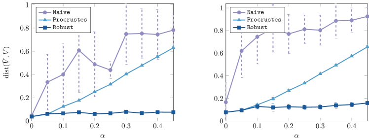
Figure 1: Robust distributed PCA with $m=150$, $n=50r$, $r_{\star}=2r$, and $\kappa=5$ under Model (24). We report the mean subspace distance $\pm$ one standard deviation over $10$ independent runs for subspace dimension $r=5$ (left) and $r=10$ (right).

4 Discussion

We presented a communication-efficient algorithm for distributed eigenspace estimation that is robust to compromised nodes returning structurally valid but otherwise potentially adversarial responses. While theory predicts that our algorithm is able to handle a constant corruption level $\alpha<\nicefrac{{1}}{{12}}$, numerical evidence suggests its breakdown point is closer to the (optimal) $\alpha_{*}=\nicefrac{{1}}{{2}}$, which might be achievable by an improved analysis of the filtering procedure in Alg 4.

Our adaptive version of the filtering procedure in Alg. 5 trades off knowledge of (an upper bound on) the corruption level $\alpha$ with the need for a precise bound on $\|\Sigma_{\mathcal{I}_{\mathsf{good}}}\|_{2}$. In the complementary situation (where such a bound on $\|\Sigma_{\mathcal{I}_{\mathsf{good}}}\|_{2}$ is known), one can design a version of Algorithm 5 that is adaptive to the corruption level $\alpha$ using a similar construction that evaluates the error proxy $f(\lambda;p,\alpha)$ for different values of $\alpha$ and fixed $\lambda\approx\|\Sigma_{\mathcal{I}_{\mathsf{good}}}\|_{2}$ instead.

Finally, we note that our algorithm suggests a natural pipeline for robustifying communication-efficient one-shot algorithms by aggregating local responses after an outlier filtering stage, which is likely applicable to other statistical problems admitting one-shot estimators in the distributed setting.

Acknowledgements

We thank Jayadev Acharya and Damek Davis for their insightful comments and suggestions.

Appendix A Auxiliary results

In this section, we present a few supporting results. The first result is a path independence lemma for perturbations of eigenvectors. It first appeared in [32]; the eigengap condition in the statement of the Lemma is justified in [8, Lemma 5].

Lemma 2 (Path independence).

Let $A\in\mathbb{R}^{d\times d}$ be a fixed symmetric matrix and let $\hat{A}:=A+E$, where $E$ is a symmetric perturbation. Suppose that we can write

$$\hat{A}-A=E_{0}+E_{1}=F_{0}+F_{1},$$

where $E_{0},E_{1},F_{0},F_{1}$ are symmetric matrices, and define the intermediate matrices

$$\hat{A}_{1}:=A+E_{0},\;\hat{A}_{2}=\hat{A}_{1}+E_{1},\quad\tilde{A}_{1}:=A+F_{0},\;\tilde{A}_{2}=\tilde{A}_{1}+F_{1}.$$

Fix any $V\in O(d,r)$ whose columns span the principal $r$-dimensional invariant subspace of $A$ and construct the leading eigenvector matrices $\hat{V}_{1}$, $\hat{V}_{2}\in O(d,r)$ of $\hat{A}_{1}$ and $\hat{A}_{2}$ such that

$$\min_{U\in\mathbb{O}_{r}}\left\|\hat{V}_{1}U-V\right\|_{F}=\left\|\hat{V}_{1}-V\right\|_{F},\quad\min_{U\in\mathbb{O}_{r}}\left\|\hat{V}_{2}U-\hat{V}_{1}\right\|_{F}=\left\|\hat{V}_{2}-\hat{V}_{1}\right\|_{F}.$$

Further, let $\tilde{V}_{1}$ and $\tilde{V}_{2}$ be the leading eigenvector matrices of $\tilde{A}_{1}$ and $\tilde{A}_{2}$, constructed in a similar fashion. Then, $\hat{V}_{2}$ and $\tilde{V}_{2}$ both span principal invariant subspaces of $\hat{A}=A+E$. Moreover, they satisfy

$$\hat{V}_{2}=\tilde{V}_{2}+T,\quad\left\|T\right\|_{2}\lesssim\frac{\varepsilon^{2}}{\delta^{2}},\quad\varepsilon:=\max\left\{\left\|E_{0}\right\|_{2},\left\|E_{1}\right\|_{2},\left\|F_{0}\right\|_{2},\left\|F_{1}\right\|_{2}\right\},$$

as long as $A$ satisfies $\delta_{r}(A)\geq 4\varepsilon$.

Lemma 3.

Suppose that $U\in\mathbb{O}_{d,r}$ satisfies $\mathrm{dist}(U,V)\leq\varepsilon<\nicefrac{{1}}{{2}}$, where $V$ is the principal eigenvector matrix of a symmetric matrix $A$ with eigengap $\delta_{r}(A):=\lambda_{r}(A)-\lambda_{r+1}(A)>0$. Then there exists a symmetric matrix $B$ such that the following hold:

1. $\left\|A-B\right\|_{2}\leq 8\left\|A\right\|_{2}\varepsilon$ and $\delta_{r}(B)=\delta_{r}(A)$.

2. $U$ is the principal eigenvector matrix of $B$.

Proof.

We prove Item 1 first. To that end, we can write $A=A_{1}+A_{2}$, where $A_{1}:=V\Sigma_{1}V^{\mathsf{T}}$ and $A_{2}:=V_{\perp}\Sigma_{2}V_{\perp}^{\mathsf{T}}$. We consider the following matrix $B$:

$$B=U\Sigma_{1}U^{\mathsf{T}}+U_{\perp}\Sigma_{2}U_{\perp}^{\mathsf{T}},$$ (25)

where $U_{\perp}^{\mathsf{T}}U=0$ and $U_{\perp}\in\mathbb{O}_{d,d-r}$. From (25) and the condition $\Sigma_{1}\succ\Sigma_{2}$, it follows that $U$ is a principal eigenvector matrix for $B$. Moreover, the gap condition on $A$ immediately translates to the claimed gap condition for $B$.

It remains to bound the distance between $A$ and $B$. We write

$$\left\|A-B\right\|_{2} \leq\left\|U\Sigma_{1}U^{\mathsf{T}}-A_{1}\right\|_{2}+\left\|U_{\perp}\Sigma_{2}U_{\perp}^{\mathsf{T}}-A_{2}\right\|_{2}.$$

To upper bound the first term on the right-hand side above, we use the spectral projectors $P_{U}:=UU^{\mathsf{T}}$ and $P_{U_{\perp}}=I-P_{U}$ to decompose it into

$$\left\|U\Sigma_{1}U^{\mathsf{T}}-A_{1}\right\|_{2} \leq\left\|U\Sigma_{1}U^{\mathsf{T}}-P_{U}A_{1}\right\|_{2}+\left\|P_{U_{\perp}}A_{1}\right\|_{2}$$

$$\leq\left\|U\Sigma_{1}U^{\mathsf{T}}-P_{U}A_{1}P_{U}\right\|_{2}+\left\|P_{U}A_{1}P_{U_{\perp}}\right\|_{2}+\left\|P_{U_{\perp}}A_{1}\right\|_{2}$$

$$\leq\left\|\Sigma_{1}-U^{\mathsf{T}}V\Sigma_{1}V^{\mathsf{T}}U\right\|_{2}+2\left\|\Sigma_{1}\right\|_{2}\left\|P_{U_{\perp}}V\right\|_{2}$$

$$\leq\left\|\Sigma_{1}(I-V^{\mathsf{T}}U)\right\|_{2}+\left\|(I-V^{\mathsf{T}}U)\Sigma_{1}V^{\mathsf{T}}U\right\|_{2}+2\left\|\Sigma_{1}\right\|_{2}\left\|P_{U_{\perp}}V\right\|_{2}$$

$$\leq 2\left\|\Sigma_{1}\right\|_{2}\varepsilon+4\left\|\Sigma_{1}\right\|_{2}\varepsilon^{2},$$

where the last inequality follows from the inequality $\left\|P_{U_{\perp}}V\right\|_{2}=\mathrm{dist}(U,V)=\varepsilon$ and Lemma 4. A similar argument shows that $\left\|U_{\perp}\Sigma_{2}U_{\perp}^{\mathsf{T}}-A_{2}\right\|_{2}\leq 2\left\|\Sigma_{2}\right\|_{2}\varepsilon+4\left\|\Sigma_{2}\right\|_{2}\varepsilon^{2}.$ Taking into account the bound $\varepsilon<1/2$ completes the proof. ∎

Lemma 4 (Modified $\sin\theta$ distance).

Let $U,V\in O(d,r)$ satisfy $\mathrm{dist}(U,V)=\alpha<1$. Then the following holds:

$$\left\|I-U^{\mathsf{T}}V\right\|_{2}\leq 2\alpha^{2}.$$

Proof.

Let $P\Sigma Q^{\mathsf{T}}$ be the singular value decomposition of $U^{\mathsf{T}}V$. Recall that [12, Eq. (2.5)]:

$$\Sigma=\mathrm{diag}\left(\sigma_{1},\dots,\sigma_{r}\right);\quad\sigma_{i}=\cos(\theta_{i}),$$

where $\theta_{i}\in[0,\pi/2]$ and $\left\|\sin\Theta\right\|_{2}=\alpha$, following [12, Lemma 2.5]. From our assumptions, it follows that

$$\left\|I-U^{\mathsf{T}}V\right\|_{2} =\left\|P(I-\Sigma)Q^{\mathsf{T}}\right\|_{2}$$

$$=\left\|I-\Sigma\right\|_{2}$$

$$=\max_{i\in[r]}\left\{1-\cos(\theta_{i})\right\}$$

$$=\max_{i\in[r]}\left\{2\sin^{2}(\theta_{i}/2)\right\}$$

$$\leq 2\,\max_{i\in[r]}\sin^{2}(\theta_{i})$$

$$=2\left\|\sin\Theta\right\|_{2}^{2},$$

with the last inequality following from $0\leq\sin(\theta/2)\leq\sin(\theta)$ for any $\theta\in[0,\pi/2]$. ∎

Appendix B Omitted proofs

This section includes proofs that were omitted from the main text.

B.1 Proof of Lemma 1

Proof.

Recall that $V$ is an eigenvector matrix of $A$ that satisfies

$$\min_{Z\in\mathbb{O}_{r}}\left\|V-V_{\mathsf{ref}}Z\right\|_{\mathrm{F}}=\left\|V-V_{\mathsf{ref}}\right\|_{\mathrm{F}}.$$

From Lemma 3, it follows that the columns of $V_{\mathsf{ref}}$ span the principal eigenspace of a matrix $B$ with nontrivial eigengap that satisfies $\left\|A-B\right\|_{2}\lesssim\left\|A\right\|_{2}\varepsilon$. We now relate $V^{\mathsf{ideal}}_{i}$ to $V_{i}^{\mathsf{corr}}$ using the aforementioned path independence result.

To that end, note that ${V}_{i}^{\mathsf{ideal}}$ is the leading eigenvector matrix of

$$A_{i}:=A+(A_{i}-A)+0,$$

that has been maximally aligned with $V$ (in the sense of Frobenius distance). On the other hand, the Procrustes estimates ${V}_{i}^{\mathsf{corr}}$ are given by the leading eigenvector matrices of

$$A_{i}:=A+(B-A)+(A_{i}-B),$$

since $V_{\mathsf{ref}}$ is the leading eigenvector of $B$ nearest to $V$ and $V_{i}^{\mathsf{corr}}$ is formed as the leading eigenvector of $A_{i}$ nearest to $V_{\mathsf{ref}}$. Applying Lemma 2 with $E_{0}:=A_{i}-A$, $E_{1}=\bm{0}$, $F_{0}:=B-A$ and $F_{1}:=A_{i}-B$, we obtain

$$V_{i}^{\mathsf{corr}}=V_{i}^{\mathsf{ideal}}+\mathcal{O}\left(\frac{1}{\delta^{2}}\max\left\{\left\|A_{i}-A\right\|_{2}^{2},\left\|B-A\right\|_{2}^{2},\left\|A_{i}-B\right\|_{2}^{2}\right\}\right).$$

Finally, we note the following upper bound

$$\left\|A_{i}-B\right\|_{2}^{2}\lesssim\left\|A_{i}-A\right\|_{2}^{2}+\left\|A-B\right\|_{2}^{2}\lesssim\max\left(\left\|A_{i}-A\right\|_{2}^{2},\left\|A\right\|_{2}^{2}\varepsilon^{2}\right),$$

which concludes the proof. ∎

B.2 Proof of Proposition 3

Proof.

Let ${j_{\mathsf{crit}}}$ be the smallest index for which $2^{j}\geq\max\left\{\lambda_{\mathsf{lb}},\left\|\Sigma_{G_{0}}\right\|_{2}\right\}$. For a fixed corruption fraction $\alpha$ and failure probability $p$, define the events

$$\mathcal{E}_{j}:=\left\{\Bigl{\|}{\theta_{2^{j}}-\frac{1}{\left|G_{0}\right|}\sum_{i\in G_{0}}X_{i}}\Bigr{\|}_{2}\leq f(2^{j};p,\alpha)\right\},\quad\mathcal{E}:=\operatorname*{\bigcap}_{j=j_{\mathsf{crit}}}^{j_{\mathsf{hi}}}\mathcal{E}_{j}.$$

From Theorem 3 in the main text and a union bound, it follows that

$$\mathbb{P}\left(\mathcal{E}\right) \geq 1-\sum_{j\in\left\{j_{\mathsf{crit}},\dots,j_{\mathsf{hi}}\right\}}\mathbb{P}\left(\Bigl{\|}{{\theta}_{2^{j}}-\frac{1}{\left|G_{0}\right|}\sum_{i\in G_{0}}X_{i}}\Bigr{\|}_{2}\geq f(2^{j};p,\alpha)\right)$$

$$\geq 1-\left(j_{\mathsf{hi}}-j_{\mathsf{crit}}\right)\cdot p$$

$$\geq 1-2\log_{2}\left(\frac{\lambda_{\mathsf{ub}}}{\lambda_{\mathsf{lb}}}\right)p.$$

Let us write $\theta_{\ast}:=\frac{1}{\left|G_{0}\right|}\sum_{i\in G_{0}}X_{i}$. Conditioned on the event $\mathcal{E}$, for any $j,j^{\prime}\geq j_{\mathsf{crit}}$ we have

$$\left\|{\theta}_{2^{j}}-{\theta}_{2^{j^{\prime}}}\right\|_{2} \leq\left\|{\theta}_{2^{j}}-\theta_{\ast}\right\|_{2}+\left\|{\theta}_{2^{j^{\prime}}}-\theta_{\ast}\right\|_{2}\leq f(2^{j};p,\alpha)+f(2^{j^{\prime}};p,\alpha).$$

Consequently, it follows that $2^{j_{\mathsf{crit}}}$ satisfies the condition of the estimator, and therefore

$$\hat{\lambda}\leq 2^{j_{\mathsf{crit}}}\leq 2\max\left\{\lambda_{\mathsf{lb}},\left\|\Sigma_{G_{0}}\right\|_{2}\right\}.$$

Finally, the desired claim follows since

$$\left\|{\theta}_{\hat{\lambda}}-\theta_{\ast}\right\|_{2} \leq\left\|{\theta}_{\hat{\lambda}}-{\theta}_{2^{j_{\mathsf{crit}}}}\right\|_{2}+\left\|{\theta}_{2^{j_{\mathsf{crit}}}}-\theta_{\ast}\right\|_{2}$$

$$\leq f(\hat{\lambda};p,\alpha)+2f(2^{j_{\mathsf{crit}}};p,\alpha)$$

$$\leq 3f(2^{j_{\mathsf{crit}}};p,\alpha)$$

$$\leq 171\sqrt{\left\|\Sigma_{G_{0}}\right\|_{2}}\left(\alpha+\frac{4\log(1/p)}{m}\right)^{1/2}.$$

∎

The next Lemma provides an upper bound on the operator norm of the empirical covariance $\Sigma_{\mathcal{I}_{\mathsf{good}}}$.

Lemma 5.

Suppose that $\widehat{V}_{\mathsf{ref}}$ satisfies $\delta_{r}(A)\geq 8\,\mathrm{dist}(\widehat{V}_{\mathsf{ref}},V)$. Then we have

$$\left\|\Sigma_{\mathcal{I}_{\mathsf{good}}}\right\|_{2}\leq\biggl{\|}{\frac{1}{\left|\mathcal{I}_{\mathsf{good}}\right|}\sum_{i\in\mathcal{I}_{\mathsf{good}}}V_{i}V_{i}^{\mathsf{T}}-VV^{\mathsf{T}}}\biggr{\|}_{2}+2\,\biggl{\|}{\frac{1}{\left|\mathcal{I}_{\mathsf{good}}\right|}\sum_{i\in\mathcal{I}_{\mathsf{good}}}\widetilde{V}_{i}-V}\biggr{\|}_{2}.$$ (26)

Proof.

Let $\mu$ denote the empirical mean over $\mathcal{I}_{\mathsf{good}}$. We have

$$\mu =\frac{1}{\left|\mathcal{I}_{\mathsf{good}}\right|}\sum_{i\in\mathcal{I}_{\mathsf{good}}}\widetilde{V}_{i},$$

$$\Sigma_{\mathcal{I}_{\mathsf{good}}} =\frac{1}{\left|\mathcal{I}_{\mathsf{good}}\right|}\sum_{i\in\mathcal{I}_{\mathsf{good}}}(\widetilde{V}_{i}-\mu)(\widetilde{V}_{i}-\mu)^{\mathsf{T}}$$

$$=\frac{1}{\left|\mathcal{I}_{\mathsf{good}}\right|}\sum_{i\in\mathcal{I}_{\mathsf{good}}}\widetilde{V}_{i}\widetilde{V}_{i}^{\mathsf{T}}-\mu\mu^{\mathsf{T}}$$

$$=\frac{1}{\left|\mathcal{I}_{\mathsf{good}}\right|}\sum_{i\in\mathcal{I}_{\mathsf{good}}}\widetilde{V}_{i}\widetilde{V}_{i}^{\mathsf{T}}-VV^{\mathsf{T}}+VV^{\mathsf{T}}-\mu\mu^{\mathsf{T}}$$

$$=\frac{1}{\left|\mathcal{I}_{\mathsf{good}}\right|}\sum_{i\in\mathcal{I}_{\mathsf{good}}}\widetilde{V}_{i}\widetilde{V}_{i}^{\mathsf{T}}-VV^{\mathsf{T}}+(V-\mu)(V+\mu)^{\mathsf{T}},$$

where $V\in\mathbb{O}_{d,r}$ spans the principal eigenspace of $A$ and satisfies

$$\min_{Z\in\mathbb{O}_{r}}\left\|VZ-\widehat{V}_{\mathsf{ref}}\right\|_{\mathrm{F}}=\left\|V-\widehat{V}_{\mathsf{ref}}\right\|_{\mathrm{F}}.$$

We now bound the spectral norm of $\Sigma_{\mathcal{I}_{\mathsf{good}}}$. Indeed, we have

$$\left\|\Sigma_{\mathcal{I}_{\mathsf{good}}}\right\|_{2} \leq\biggl{\|}{\frac{1}{\left|\mathcal{I}_{\mathsf{good}}\right|}\sum_{i\in\mathcal{I}_{\mathsf{good}}}\widetilde{V}_{i}\widetilde{V}_{i}^{\mathsf{T}}-VV^{\mathsf{T}}}\biggr{\|}_{2}+\left\|V+\mu\right\|_{2}\biggl{\|}{\frac{1}{\left|\mathcal{I}_{\mathsf{good}}\right|}\sum_{i\in\mathcal{I}_{\mathsf{good}}}\widetilde{V}_{i}-V}\biggr{\|}_{2}$$

$$\leq\biggl{\|}{\frac{1}{\left|\mathcal{I}_{\mathsf{good}}\right|}\sum_{i\in\mathcal{I}_{\mathsf{good}}}V_{i}V_{i}^{\mathsf{T}}-VV^{\mathsf{T}}}\biggr{\|}_{2}+2\,\biggl{\|}{\frac{1}{\left|\mathcal{I}_{\mathsf{good}}\right|}\sum_{i\in\mathcal{I}_{\mathsf{good}}}\widetilde{V}_{i}-V}\biggr{\|}_{2},$$

using the fact that $\widetilde{V}_{i}\widetilde{V}_{i}^{\mathsf{T}}=V_{i}V_{i}^{\mathsf{T}}$ for all $i\in\mathcal{I}_{\mathsf{good}}$. ∎

B.3 Proof of Theorem 3

In this section, we modify the proof of [30, Theorem 4] to derive guarantees for robust mean estimation with matrix-valued inputs. We recall some notation used therein: given the set of “good” samples $G_{0}$ and the initial sample $S_{0}=\left\{1,\dots,m\right\}$, we denote

$$S_{k} =\left\{\text{points remaining after $k$ recursive calls to {Filter}}\right\},$$ (27)

$$G_{k} =S_{k}\cap G_{0},$$

$$B_{k} =S_{k}\setminus G_{0},$$

$$\alpha =\frac{m-\left|G_{0}\right|}{m}.$$

Moreover, given any set $S\subset[m]$, we write

$$\Sigma_{S}:=\frac{1}{\left|S\right|}\sum_{i\in S}(X_{i}-\mu_{S})(X_{i}-\mu_{S})^{\mathsf{T}},\quad\text{where}\quad\mu_{S}:=\frac{1}{\left|S\right|}\sum_{i\in S}X_{i}.$$ (28)

In our proofs, we frequently employ the total variation distance $d_{\mathrm{TV}}$. For discrete distributions $P_{1}$, $P_{2}$ on a common sample space $\Omega$, $d_{\mathrm{TV}}$ is given by

$$d_{\mathrm{TV}}(P_{1},P_{2})=\frac{1}{2}\left\|P_{1}-P_{2}\right\|_{1}=\frac{1}{2}\sum_{x\in\Omega}\left|P_{1}(x)-P_{2}(x)\right|.$$ (29)

Finally, we define the events $\mathcal{E}_{k}$, where $k\in\mathbb{N}$, as below:

$$\mathcal{E}_{k}:=\left\{\sum_{i\in G_{k}}\tau_{i}\geq\frac{1}{\gamma}\sum_{j\in S_{k}}\tau_{j}\right\},\quad k=0,1,\dots$$ (30)

Our proof essentially traces the proof of [30, Theorem 4] but for the case of matrix-valued inputs to the Filter algorithm. The first result has already been shown in [30], as its proof is independent of the shape of the inputs.

Lemma 6 (See [30, Lemma 6]).

Let $T:=\inf\left\{k\in\mathbb{N}\ \middle|\ \text{$\mathcal{E}_{k}$ is true}\right\}$. Then we have:

$$\mathbb{P}\left(T\geq 3(m-\left|G_{0}\right|)+18\log(1/p)\right)\leq p.$$ (31)

The remainder of the proof is devoted to showing that, as soon as some $\mathcal{E}_{k}$ is true, Filter will terminate with a good estimate. Throughout, we condition on the event

$$\mathcal{E}:=\left\{T\leq T_{p}\right\},\quad\text{where}\quad T_{p}:=3(m-\left|G_{0}\right|)+18\log(1/p),$$ (32)

which holds with probability at least $1-p$.

Theorem 5.

Suppose that $\alpha$, $p$ and $N$ satisfy

$$3\alpha+\frac{18\log(1/p)}{m}\leq\frac{1}{4}.$$ (33)

Then the following hold simultaneously with probability at least $1-p$:

1. $\mathtt{Filter}(S_{0},\left\|\Sigma_{G_{0}}\right\|_{2})$ terminates after at most $T_{p}$ iterations;

2. The output of $\mathtt{Filter}(S_{0},\left\|\Sigma_{G_{0}}\right\|_{2})$, ${\theta}_{\left\|\Sigma_{G_{0}}\right\|_{2}}$, satisfies

   $$\Bigl{\|}{{\theta}_{\left\|\Sigma_{G_{0}}\right\|_{2}}-\frac{1}{\left|G_{0}\right|}\sum_{i\in G_{0}}X_{i}}\Bigr{\|}_{2}\leq 18\sqrt{5\left\|\Sigma_{G_{0}}\right\|_{2}}\left(\alpha+\frac{4\log(1/p)}{m}\right)^{1/2}.$$ (34)

Remark 3.

While we prove the Theorem for the case $\lambda_{\mathsf{ub}}=\left\|\Sigma_{G_{0}}\right\|_{2}$, a straightforward modification of the proof shows that when $\lambda_{\mathsf{ub}}\geq\left\|\Sigma_{G_{0}}\right\|_{2}$, we have

$$\Bigl{\|}{\theta_{\lambda_{\mathsf{ub}}}-\frac{1}{\left|G_{0}\right|}\sum_{i\in G_{0}}X_{i}}\Bigr{\|}_{2}\leq 18\sqrt{5\lambda_{\mathsf{ub}}}\left(\alpha+\frac{4\log(1/p)}{m}\right)^{1/2}.$$

Proof of Theorem 5.

We condition on the event $\mathcal{E}$ from (32), which holds with probability at least $1-p$. This implies that there is some index $k\leq T_{p}$ such that

$$\sum_{i\in G_{k}}\tau_{i}\geq\frac{1}{\gamma}\sum_{j\in S_{k}}\tau_{j}.$$

From Lemma 11, we obtain that the empirical covariance satisfies $\left\|\Sigma_{S_{k}}\right\|_{2}\leq 18\left\|\Sigma_{G_{0}}\right\|_{2},$ and thus the algorithm terminates after at most $k$ steps. We have the following cases:

1. The termination condition was first triggered at the $k^{\text{th}}$ step. In that case, Lemma 11 directly implies the desired inequality.

2. The algorithm terminated at some index $\ell<k$. Then it follows from Lemma 12 that

   $$\eta:=d_{\mathrm{TV}}(\mathrm{Unif}(S_{\ell}),\mathrm{Unif}(G_{0}))\leq 5\alpha+\frac{20\log(1/p)}{N}.$$ (35)

   At the same time, Lemma 7 implies that

   $$\Bigl{\|}{{\theta}_{\left\|\Sigma_{G_{0}}\right\|_{2}}-\frac{1}{\left|G_{0}\right|}\sum_{i\in G_{0}}X_{i}}\Bigr{\|}_{2}\leq\frac{\sqrt{\eta}}{1-\sqrt{\eta}}\cdot\left(\left\|\Sigma_{S_{\ell}}\right\|_{2}^{1/2}+\left\|\Sigma_{G_{0}}\right\|_{2}^{1/2}\right).$$ (36)

   From the termination condition, we obtain that

   $$\left\|\Sigma_{S_{\ell}}\right\|_{2}\leq 18\left\|\Sigma_{G_{0}}\right\|_{2}.$$ (37)

   Combining Eqs. 35, 36 and 37 yields the desired bound.

∎

The next few Lemmas are supporting statements used in the proof of Theorem 5.

Lemma 7.

Let $S=\left\{X_{1},\dots,X_{m}\right\}$ where $X_{i}\in\mathbb{R}^{d\times r}$ and suppose that $P_{1}$, $P_{2}$ are discrete distributions supported over $[m]$ with $d_{\mathrm{TV}}(P_{1},P_{2})=\eta$. Then the following holds:

$$\left\|\mathbb{E}_{P_{1}}\left[X_{i}\right]-\mathbb{E}_{P_{2}}\left[X_{i}\right]\right\|_{2}\leq\frac{\sqrt{\eta}}{1-\sqrt{\eta}}\cdot\left(\left\|\Sigma_{P_{1}}\right\|_{2}^{1/2}+\left\|\Sigma_{P_{2}}\right\|_{2}^{1/2}\right),$$ (38)

where the matrices $\Sigma_{P_{i}}$ are defined as:

$$\Sigma_{P_{i}}=\mathbb{E}_{X\sim P_{i}}\left[(X-\mathbb{E}_{P_{i}}\left[X\right])(X-\mathbb{E}_{P_{i}}\left[X\right])^{\mathsf{T}}\right].$$

Proof.

Following the proof of [24, Lemma 2.1], we consider a coupling between $P_{1}$ and $P_{2}$ such that $\mathbb{P}\left(X=X^{\prime}\right)\geq 1-\eta$. Denoting $\left\|X\right\|_{L^{2}}:=\sqrt{\mathbb{E}\left[X^{2}\right]}$, we have

$$\left\|\mathbb{E}_{P_{1}}\left[X\right]-\mathbb{E}_{P_{2}}\left[X^{\prime}\right]\right\|_{2} =\sup_{u,v\in\mathcal{B}}\left\langle u,(\mathbb{E}_{P_{1}}\left[X\right]-\mathbb{E}_{P_{2}}\left[X^{\prime}\right])v\right\rangle$$

$$=\sup_{u,v\in\mathcal{B}}\mathbb{E}\left[\left\langle u,(X-X^{\prime})v\right\rangle\bm{1}\left\{X\neq X^{\prime}\right\}\right]$$

$$\leq\mathbb{E}\left[\bm{1}\left\{X\neq X^{\prime}\right\}^{2}\right]^{1/2}\cdot\sup_{u,v\in\mathcal{B}}\mathbb{E}\left[\left\langle u,(X-X^{\prime})v\right\rangle^{2}\right]^{1/2}$$

$$\leq\sqrt{\eta}\cdot\sup_{u,v\in\mathcal{B}}\left\|\left\langle u,(X-X^{\prime})v\right\rangle\right\|_{L^{2}}.$$ (39)

Let $\mu_{1}:=\mathbb{E}_{P_{1}}\left[X\right]$ and $\mu_{2}=\mathbb{E}_{P_{2}}\left[X\right]$. Since $\left\|\cdot\right\|_{L^{2}}$ is a norm, the triangle inequality implies that

$$\sup_{u,v\in\mathcal{B}}\left\|\left\langle u,(X-X^{\prime})v\right\rangle\right\|_{L^{2}} =\sup_{u,v\in\mathcal{B}}\left\|\left\langle u,(X-\mu_{1}+\mu_{1}-\mu_{2}+\mu_{2}-X^{\prime})v\right\rangle\right\|_{L^{2}}$$

$$\leq\begin{aligned} &\sup_{u,v\in\mathcal{B}}\left\|\left\langle u,(X-\mu_{1})v\right\rangle\right\|_{L^{2}}+\sup_{u,v\in\mathcal{B}}\left\|\left\langle u,(X^{\prime}-\mu_{2})v\right\rangle\right\|_{L^{2}}\\ &+\sup_{u,v\in\mathcal{B}}\left\|\left\langle u,(\mu_{1}-\mu_{2})v\right\rangle\right\|_{L^{2}}.\end{aligned}$$ (40)

We now upper bound the remaining terms. For the first one, we have

$$\sup_{u,v\in\mathcal{B}}\left\|\left\langle u,(X-\mu_{1})v\right\rangle\right\|_{L^{2}} =\sup_{u,v\in\mathcal{B}}\mathbb{E}\left[\left\langle u,(X-\mu_{1})v\right\rangle^{2}\right]^{1/2}$$

$$=\sup_{u,v\in\mathcal{B}}\mathbb{E}\bigl{[}\mathrm{Tr}\bigl{(}u^{\mathsf{T}}(X-\mu_{1})\underbrace{vv^{\mathsf{T}}}_{\preceq I_{d}}(X-\mu_{1})^{\mathsf{T}}u\bigr{)}\bigr{]}^{1/2}$$

$$\leq\sup_{u\in\mathcal{B}}\mathbb{E}\left[\mathrm{Tr}\left(u^{\mathsf{T}}(X-\mu_{1})(X-\mu_{1})^{\mathsf{T}}u\right)\right]^{1/2}$$

$$=\left(\sup_{u\in\mathcal{B}}\left\langle u,\mathbb{E}\left[(X-\mu_{1})(X-\mu_{1})^{\mathsf{T}}\right]u\right\rangle\right)^{1/2}$$

$$=\left\|\Sigma_{P_{1}}\right\|_{2}^{1/2},$$ (41)

where the penultimate equality uses linearity of the trace operator and the last equality is the definition of the spectral norm for symmetric positive semidefinite matrices. Similar arguments also yield

$$\sup_{u,v\in\mathcal{B}}\left\|\left\langle u,(X^{\prime}-\mu_{2})v\right\rangle\right\|_{L^{2}} \leq\left\|\Sigma_{P_{2}}\right\|_{2}^{1/2},$$ (42)

$$\sup_{u,v\in\mathcal{B}}\left\|\left\langle u,(\mu_{1}-\mu_{2})v\right\rangle\right\|_{L^{2}} \leq\left\|\mathbb{E}_{P_{1}}\left[X\right]-\mathbb{E}_{P_{2}}\left[X^{\prime}\right]\right\|_{2}.$$ (43)

Plugging Eqs. 40, 41, 42 and 43 back into Eq. 39 and rearranging yields the expected result:

$$\left\|\mathbb{E}_{P_{1}}\left[X\right]-\mathbb{E}_{P_{2}}\left[X^{\prime}\right]\right\|_{2}\leq\frac{\sqrt{\eta}}{1-\sqrt{\eta}}\left(\left\|\Sigma_{P_{1}}\right\|_{2}^{1/2}+\left\|\Sigma_{P_{2}}\right\|_{2}^{1/2}\right).$$

∎

Lemma 8.

Let $G\subset S\subset[m]$. Moreover, let $\mu_{S}$ and $\mu_{G}$ be their respective empirical means, and let $v$ be the leading eigenvector of $\Sigma_{S}$ so that the outlier scores satisfy

$$\tau_{i}=\left\langle v,(X_{i}-\mu_{S})(X_{i}-\mu_{S})^{\mathsf{T}}v\right\rangle,\quad\forall i\in S.$$

Moreover, define $\eta:=1-\nicefrac{{\left|G\right|}}{{\left|S\right|}}$ and fix a $\gamma\in(0,\nicefrac{{1}}{{\eta}})$. Then, we have the implication

$$\left\|\Sigma_{S}\right\|_{2}\geq(1-\eta)^{2}\left(\frac{\gamma}{1-\gamma\eta}\right)\left\|\Sigma_{G}\right\|_{2}\implies\sum_{j\in G}\tau_{j}\leq\frac{1}{\gamma}\sum_{i\in S}\tau_{i}.$$ (44)

Proof.

Recall that the (normalized) sum of outlier scores over the set $G$ is given by

$$\frac{1}{\left|G\right|}\left\langle v,\sum_{i\in G}(X_{i}-\mu_{S})(X_{i}-\mu_{S})^{\mathsf{T}}v\right\rangle =\begin{aligned} &\frac{1}{\left|G\right|}\left\langle v,\sum_{i\in G}(X_{i}-\mu_{G})(X_{i}-\mu_{G})^{\mathsf{T}}v\right\rangle\\ &+\left\langle v,(\mu_{S}-\mu_{G})(\mu_{S}-\mu_{G})^{\mathsf{T}}v\right\rangle\end{aligned}$$

$$=\left\langle v,\Sigma_{G}v\right\rangle+\left\langle v,(\mu_{S}-\mu_{G})(\mu_{S}-\mu_{G})^{\mathsf{T}}v\right\rangle.$$ (45)

We now simplify the second term. Indeed, we have

$$\mu_{S}-\mu_{G} =\frac{1}{\left|S\right|}\sum_{i\in G}X_{i}+\frac{1}{\left|S\right|}\sum_{i\in S\setminus G}X_{i}-\frac{1}{\left|G\right|}\sum_{i\in G}X_{i}$$

$$=\left(1-\frac{\left|G\right|}{\left|S\right|}\right)\left(\mu_{S\setminus G}-\mu_{G}\right)$$ (46)

For brevity, denote $\eta:=\frac{\left|S\setminus G\right|}{\left|S\right|}$. Plugging (46) back into (45), we obtain

$$\frac{1}{\left|G\right|}\sum_{j\in G}\tau_{j} =\left\langle v,\Sigma_{G}v\right\rangle+\eta^{2}\left\langle v,(\mu_{S\setminus G}-\mu_{G})(\mu_{S\setminus G}-\mu_{G})^{\mathsf{T}}v\right\rangle$$ (47)

We now bound the second term in (47). From [14, Lemma 2.4], it follows that

$$\left\langle v,\Sigma_{S}v\right\rangle =\left(1-\eta\right)\left\langle v,\Sigma_{G}v\right\rangle+\eta\left\langle v,\Sigma_{S\setminus G}v\right\rangle+\eta(1-\eta)\left\langle v,(\mu_{S\setminus G}-\mu_{G})(\mu_{S\setminus G}-\mu_{G})^{\mathsf{T}}v\right\rangle$$

Rearranging and multiplying by $\eta/(1-\eta)$ gives

$$\eta^{2}\left\langle v,(\mu_{S\setminus G}-\mu_{G})(\mu_{S\setminus G}-\mu_{G})^{\mathsf{T}}v\right\rangle =\frac{\eta}{1-\eta}\left\langle v,\Sigma_{S}v\right\rangle-\eta\left\langle v,\Sigma_{G}v\right\rangle-\frac{\eta^{2}}{(1-\eta)}\left\langle v,\Sigma_{S\setminus G}v\right\rangle$$

$$\leq\frac{\eta}{1-\eta}\left\langle v,\Sigma_{S}v\right\rangle-\eta\left\langle v,\Sigma_{G}v\right\rangle.$$

Plugging back into Eq. 47 and using the fact that $\left|G\right|=\left|S\right|(1-\eta)$, we obtain

$$\sum_{j\in G}\tau_{j} \leq\left|G\right|(1-\eta)\left\langle v,\Sigma_{G}v\right\rangle+\frac{\left|G\right|\eta}{1-\eta}\left\langle v,\Sigma_{S}v\right\rangle$$

$$\leq\left|G\right|(1-\eta)\left\|\Sigma_{G}\right\|_{2}+(\left|S\right|-\left|G\right|)\left|S\right|\left\|\Sigma_{S}\right\|_{2}$$ (48)

Finally, replacing $\left|G\right|=\left|S\right|(1-\eta)$ in (48) and rearranging, we obtain

$$\left\|\Sigma_{G}\right\|_{2}\leq\left(\gamma^{-1}-\eta\right)\frac{\left\|\Sigma_{S}\right\|_{2}}{(1-\eta)^{2}}\implies\sum_{j\in G}\tau_{j}\leq\frac{1}{\gamma}\sum_{i\in S}\tau_{i}.$$

∎

Lemma 9.

Suppose that (33) is true. Then the following holds for any $k\leq T_{p}$:

$$\frac{\left|S_{k}\setminus G_{k}\right|}{\left|S_{k}\right|}\leq\frac{4\alpha}{3}.$$

Proof.

Recall that $B_{k}=S_{k}\setminus G_{k}$ and notice that

$$\frac{\left|B_{k}\right|}{\left|S_{k}\right|} =\frac{\left|B_{k}\right|}{\left|S_{0}\right|}\frac{\left|S_{0}\right|}{\left|S_{k}\right|}\leq\frac{\left|B_{0}\right|}{\left|S_{0}\right|}\frac{\left|S_{0}\right|}{\left|S_{0}\right|-T_{p}}=\alpha\cdot\frac{1}{1-(3\alpha+\frac{18\log(1/p)}{m})}\leq\frac{4\alpha}{3},$$

where the first inequality follows from the fact that $\left|B_{k}\right|\leq\left|B_{0}\right|$. ∎

Lemma 10.

For any integer $k$, the sets $G_{k}$ and $G_{0}$ satisfy

$$\left\|\Sigma_{G_{k}}\right\|_{2}\leq\frac{\left|G_{0}\right|}{\left|G_{k}\right|}\left\|\Sigma_{G_{0}}\right\|_{2}$$ (49)

Proof.

We expand the definition of $\Sigma_{G_{0}}$ and rewrite:

$$\Sigma_{G_{0}} =\frac{1}{\left|G_{0}\right|}\sum_{i\in G_{0}}(X_{i}-\mu_{G_{0}})(X_{i}-\mu_{G_{0}})^{\mathsf{T}}$$

$$=\underbrace{\frac{1}{\left|G_{0}\right|}\sum_{i\in G_{k}}(X_{i}-\mu_{G_{0}})(X_{i}-\mu_{G_{0}})^{\mathsf{T}}}_{T_{1}}+\underbrace{\frac{1}{\left|G_{0}\right|}\sum_{i\in G_{0}\setminus G_{k}}(X_{i}-\mu_{G_{0}})(X_{i}-\mu_{G_{0}})^{\mathsf{T}}}_{T_{2}}$$

We now rewrite the first term in the above sum using

$$T_{1} =\frac{1}{\left|G_{0}\right|}\sum_{i\in G_{k}}(X_{i}-\mu_{G_{k}}+\mu_{G_{k}}-\mu_{G_{0}})(X_{i}-\mu_{G_{k}}+\mu_{G_{k}}-\mu_{G_{0}})^{\mathsf{T}}$$

$$=\begin{aligned} &\frac{\left|G_{k}\right|}{\left|G_{0}\right|}\Sigma_{G_{k}}+\frac{\left|G_{k}\right|}{\left|G_{0}\right|}\left(\frac{1}{\left|G_{k}\right|}\sum_{i\in G_{k}}(X_{i}-\mu_{G_{k}})\right)(\mu_{G_{k}}-\mu_{G_{0}})^{\mathsf{T}}\\ &+\frac{\left|G_{k}\right|}{\left|G_{0}\right|}(\mu_{G_{k}}-\mu_{G_{0}})\left(\frac{1}{\left|G_{k}\right|}\sum_{i\in G_{k}}X_{i}-\mu_{G_{k}}\right)^{\mathsf{T}}+\frac{\left|G_{k}\right|}{\left|G_{0}\right|}(\mu_{G_{k}}-\mu_{G_{0}})(\mu_{G_{k}}-\mu_{G_{0}})^{\mathsf{T}}\end{aligned}$$

$$=\frac{\left|G_{k}\right|}{\left|G_{0}\right|}\left(\Sigma_{G_{k}}+(\mu_{G_{k}}-\mu_{G_{0}})(\mu_{G_{k}}-\mu_{G_{0}})^{\mathsf{T}}\right)$$

Letting $v\in\mathbb{S}^{d-1}$ and using the fact that $T_{2}$ is positive semidefinite, we arrive at

$$\left\langle v,\Sigma_{G_{0}}v\right\rangle=\frac{\left|G_{k}\right|}{\left|G_{0}\right|}\left(\left\langle v,\Sigma_{G_{k}}v\right\rangle+\left\|(\mu_{G_{k}}-\mu_{G_{0}})^{\mathsf{T}}v\right\|^{2}\right)+\left\langle v,T_{2}v\right\rangle\geq\frac{\left|G_{k}\right|}{\left|G_{0}\right|}\left\langle v,\Sigma_{G_{k}}v\right\rangle$$ (50)

Finally, taking suprema over both sides yields the desired inequality. ∎

Lemma 11.

Suppose that (33) is true and that the following inequality holds for some index $k\leq T_{p}$:

$$\sum_{i\in G_{k}}\tau_{i}\geq\frac{1}{\gamma}\sum_{j\in S_{k}}\tau_{j}.$$ (51)

Then the empirical means satisfy

$$\left\|\mathbb{E}_{\mathrm{Unif}(G_{0})}\left[X\right]-\mathbb{E}_{\mathrm{Unif}(S_{k})}\left[X\right]\right\|_{2}\leq 18\left(5\alpha+\frac{20\log(1/p)}{m}\right)^{1/2}\left\|\Sigma_{G_{0}}\right\|_{2}^{1/2}.$$

Proof.

Let $P_{1}:=\mathrm{Unif}(G_{0})$ and $P_{2}:=\mathrm{Unif}(S_{k})$. From Lemma 7, it follows that

$$\left\|\mathbb{E}_{P_{1}}\left[X\right]-\mathbb{E}_{P_{2}}\left[X\right]\right\|_{2}\leq\frac{\sqrt{d_{\mathrm{TV}}(P_{1},P_{2})}}{1-\sqrt{d_{\mathrm{TV}}(P_{1},P_{2})}}\cdot\left(\left\|\Sigma_{G_{0}}\right\|_{2}^{1/2}+\left\|\Sigma_{G_{k}}\right\|_{2}^{1/2}\right).$$ (52)

Since (51) is the reverse of (44), we obtain

$$\left\|\Sigma_{S_{k}}\right\|_{2} \leq(1-\eta)^{2}\frac{\gamma}{1-\gamma\eta}\left\|\Sigma_{G_{k}}\right\|_{2}$$

$$\leq\frac{3}{1-6\alpha}\left\|\Sigma_{G_{k}}\right\|_{2}$$

$$\leq 6\cdot\frac{\left|G_{0}\right|}{\left|G_{k}\right|}\left\|\Sigma_{G_{0}}\right\|_{2},$$

where the first inequality follows from the contrapositive of Lemma 8, the second inequality from $\gamma=3$ and Lemma 9, and the last inequality follows by our assumption on $\alpha$. Now, let $K\leq T_{p}$ be the number of samples in $G_{0}$ that were removed by the algorithm. We have

$$\frac{\left|G_{0}\right|}{\left|G_{k}\right|} =\frac{m-\left|B_{0}\right|}{m-\left|B_{0}\right|-K}\leq\frac{m-\left|B_{0}\right|}{m-\left|B_{0}\right|-T_{p}}\leq\frac{m-\left|B_{0}\right|}{m-18\log(1/p)-4\left|B_{0}\right|}=\frac{1-\alpha}{1-4\alpha-\frac{18\log(1/p)}{m}}$$

From (33), we additionally have that

$$1-(4\alpha+\frac{18\log(1/p)}{m})\geq 1-\frac{4}{3}\left(3\alpha+\frac{18\log(1/p)}{m}\right)\geq\frac{1}{3}\implies\left\|\Sigma_{S_{k}}\right\|_{2}\leq 18\left\|\Sigma_{G_{0}}\right\|_{2}.$$

Substituting the above into (52) and using Lemma 12 yields the desired bound:

$$\left\|\mathbb{E}_{P_{1}}\left[X\right]-\mathbb{E}_{P_{2}}\left[X\right]\right\|_{2} \leq\frac{\left(5\alpha+\frac{20\log(1/p)}{m}\right)^{1/2}}{1-\left(5\alpha+\frac{20\log(1/p)}{m}\right)^{1/2}}\left(\left\|\Sigma_{G_{0}}\right\|_{2}^{1/2}+\sqrt{18}\left\|\Sigma_{G_{0}}\right\|_{2}^{1/2}\right)$$

$$\leq 18\left(5\alpha+\frac{20\log(1/p)}{m}\right)^{1/2}\left\|\Sigma_{G_{0}}\right\|_{2}^{1/2}.$$

∎

Lemma 12.

Suppose $k\leq T_{p}$ and (33) holds. Then we have that

$$d_{\mathrm{TV}}(\mathrm{Unif}(S_{k}),\mathrm{Unif}(G_{0}))\leq 5\alpha+\frac{20\log(1/p)}{m}.$$ (53)

Proof.

We let $P_{1}:=\mathrm{Unif}(S_{k})$, $P_{2}:=\mathrm{Unif}(G_{0})$ and $P_{3}:=\mathrm{Unif}(G_{k})$, and write $K\leq k\leq T_{p}$ for the number of samples originally in $G_{0}$ that were removed by the Filter algorithm by the $k^{\text{th}}$ step. From the triangle inequality, it follows that

$$d_{\mathrm{TV}}(P_{1},P_{2}) \leq d_{\mathrm{TV}}(P_{1},P_{3})+d_{\mathrm{TV}}(P_{2},P_{3})$$

$$=\frac{\left|S_{k}\right|-\left|G_{k}\right|}{\left|S_{k}\right|}+\frac{\left|G_{0}\right|-\left|G_{k}\right|}{\left|G_{0}\right|}$$

$$=\frac{m-k-(m-\left|B_{0}\right|-K)}{m-k}+\frac{K}{m-\left|B_{0}\right|}$$

$$=\frac{\left|B_{0}\right|+(K-k)}{m-k}+\frac{K}{m-\left|B_{0}\right|}$$

$$\leq\frac{\left|B_{0}\right|}{m-k}+\frac{T_{p}}{m-\left|B_{0}\right|}$$

$$\leq\frac{\left|B_{0}\right|}{m-T_{p}}+\frac{T_{p}}{m-\left|B_{0}\right|},$$

where the second line follows from Lemma 13 and the last two inequalities follow from $K\leq m$ and $m\leq T_{p}$. Finally, using Lemma 6 and Eq. 33, we obtain

$$\frac{\left|B_{0}\right|}{m-T_{p}}+\frac{T_{p}}{m-\left|B_{0}\right|} =\frac{\alpha}{1-\frac{T_{p}}{m}}+\frac{\frac{T_{p}}{m}}{1-\alpha}$$

$$\leq\frac{\alpha}{1-\frac{18\log(1/p)}{m}-3\alpha}+\frac{\frac{18\log(1/p)}{m}+3\alpha}{1-\alpha}$$

$$\leq\frac{4\alpha}{3}+\frac{\frac{18\log(1/p)}{m}+3\alpha}{1-\alpha}$$

$$\leq\frac{4\alpha}{3}+\frac{\frac{18\log(1/p)}{m}+3\alpha}{1-\frac{1}{12}}$$

$$\leq 5\alpha+\frac{20\log(1/p)}{m}.$$

∎

Lemma 13.

Consider a pair of discrete sets $S,S^{\prime}$ such that $S^{\prime}\subset S$. We have:

$$d_{\mathrm{TV}}(\mathrm{Unif}(S),\mathrm{Unif}(S^{\prime}))=\frac{\left|S\right|-\left|S^{\prime}\right|}{\left|S\right|}.$$ (54)

Proof.

Using the fact that $d_{\mathrm{TV}}(p,q)=\frac{1}{2}\left\|p-q\right\|_{1}$, we have:

$$d_{\mathrm{TV}}(\mathrm{Unif}(S),\mathrm{Unif}(S^{\prime})) =\frac{1}{2}\left(\sum_{x\in S\cap S^{\prime}}\left|\frac{1}{\left|S\right|}-\frac{1}{\left|S^{\prime}\right|}\right|+\sum_{x\in S\setminus S^{\prime}}\frac{1}{\left|S\right|}\right)$$

$$=\frac{1}{2}\left(1-\frac{\left|S^{\prime}\right|}{\left|S\right|}+\frac{\left|S\right|-\left|S^{\prime}\right|}{\left|S\right|}\right)$$

$$=1-\frac{\left|S^{\prime}\right|}{\left|S\right|}.$$

∎

B.4 Proof of Theorem 4

We now present the proof of the main theorem on distributed PCA. We first recall that

$$A_{i}=\frac{1}{n}\sum_{j=1}^{n}X_{j}^{(i)}(X_{j}^{(i)})^{\mathsf{T}};\quad i\in\mathcal{I}_{\mathsf{good}},$$

where $X_{j}^{(i)}\overset{\mathrm{iid}}{\sim}\mathcal{P}$, and that the responses $V_{i}\in\mathbb{O}_{d,r}$ span the leading $r$-dimensional eigenspace of $A_{i}$. Under this model, the local errors $E_{i}:=A_{i}-A$ as well as the error of the empirical average over the inliers are bounded with high probability. We will condition on the following events for the remainder of this section:

$$\mathcal{E}_{1} =\left\{\max_{i\in\mathcal{I}_{\mathsf{good}}}\left\|A_{i}-A\right\|_{2}\leq\min\left\{\frac{\delta}{8},C_{1}\left\|A\right\|_{2}\sqrt{\frac{r_{\star}+\log(m/p)}{n}}\right\}\right\},$$ (55)

$$\mathcal{E}_{2} =\left\{\biggl{\|}{\frac{1}{\left|\mathcal{I}_{\mathsf{good}}\right|}\sum_{i\in\mathcal{I}_{\mathsf{good}}}A_{i}-A}\biggr{\|}_{2}\leq C_{2}\left\|A\right\|_{2}\sqrt{\frac{r_{\star}+\log(n)}{\left|\mathcal{I}_{\mathsf{good}}\right|n}}\right\}.$$

Lemma 14.

Suppose that $n\gtrsim\kappa^{2}\cdot(r_{\star}+\log(mn/p))$. Then the following hold:

$$\mathbb{P}\left(\mathcal{E}_{1}\right)\leq p,\quad\mathbb{P}\left(\mathcal{E}_{2}\right)\leq\frac{2}{n}.$$ (56)

Proof.

The bound on $\mathbb{P}\left(\mathcal{E}_{2}\right)$ in Eq. 56 follows from an application of [33, Exercise 9.2.5] and the assumed lower bound on $n$. On the other hand, the same result yields

$$\mathbb{P}\left(\left\|A_{i}-A\right\|_{2}\geq C_{1}\left\|A\right\|_{2}\left(\sqrt{\frac{r_{\star}+\log(m/p)}{n}}+\frac{r_{\star}+\log(m/p)}{n}\right)\right)\leq\frac{p}{m},$$

for any fixed $i\in\mathcal{I}_{\mathsf{good}}$. From the lower bound on $n$, it follows that

$$\frac{r_{\star}+\log(m/p)}{n}\leq\sqrt{\frac{r_{\star}+\log(m/p)}{n}}\quad\text{and}\quad C_{1}\left\|A\right\|_{2}\sqrt{\frac{r_{\star}+\log(m/p)}{n}}<\frac{\delta}{8}.$$

Finally, taking a union bound over $\mathcal{I}_{\mathsf{good}}$ recovers the bound on $\mathbb{P}\left(\mathcal{E}_{1}\right)$. ∎

An immediate corollary is a bound on the error of RobustReferenceEstimator.

Corollary 2.

There is a universal constant $C_{\mathsf{ref}}$ such that the output of Alg. 2 satisfies

$$\mathrm{dist}(\widehat{V}_{\mathsf{ref}},V)\leq C_{\mathsf{ref}}\kappa\cdot\sqrt{\frac{r_{\star}+\log(m/p)}{n}}.$$

Proof.

From the bound $\alpha<\frac{1}{2}$ and the conditioning on $\mathcal{E}_{1}$, we deduce the existence of an index set $S^{\prime}$ such that $\left|S^{\prime}\right|>\frac{m}{2}$, and

$$\mathrm{dist}(\widehat{V}_{i},V)\leq\frac{\left\|A_{i}-A\right\|_{2}}{\delta-\frac{\delta}{4}}\leq\frac{2C_{1}\left\|A\right\|_{2}}{\delta}\sqrt{\frac{r_{\star}+\log(m/p)}{n}},\quad\text{for all $i\in S^{\prime}$},$$

where the first bound on $\mathrm{dist}(\widehat{V}_{i},V)$ follows from the Davis-Kahan theorem [12, Theorem 2.7] and the fact that $\left\|A_{i}-A\right\|_{2}\leq\frac{\delta}{8}$ for any $i\notin\mathcal{I}_{\mathrm{bad}}$. From Proposition 1 in the main text, it follows that

$$\mathrm{dist}(\widehat{V}_{\mathsf{ref}},V)\leq\underbrace{6C_{1}}_{C_{\mathsf{ref}}}\frac{\left\|A\right\|_{2}}{\delta}\sqrt{\frac{r_{\star}+\log(m/p)}{n}}.$$

∎

The next Proposition instantiates the bounds of Lemma 5 for for the case of distributed PCA.

Proposition 4.

In the setting of Lemma 5, the matrix $\Sigma_{\mathcal{I}_{\mathsf{good}}}$ satisfies

$$\left\|\Sigma_{\mathcal{I}_{\mathsf{good}}}\right\|_{2} \lesssim\kappa\,\sqrt{\frac{r(r_{\star}+\log(n))}{(1-\alpha)mn}}+\kappa^{2}\cdot\frac{\sqrt{r}(r_{\star}+\log(n))}{n}+\kappa^{4}\cdot\frac{r_{\star}+\log(m/p)}{n}.$$ (57)

Proof.

From Lemma 5, it follows that

$$\left\|\Sigma_{\mathcal{I}_{\mathsf{good}}}\right\|_{2} \leq\biggl{\|}{\frac{1}{\left|\mathcal{I}_{\mathsf{good}}\right|}\sum_{i\in\mathcal{I}_{\mathsf{good}}}V_{i}V_{i}^{\mathsf{T}}-VV^{\mathsf{T}}}\biggr{\|}_{2}+2\cdot\biggl{\|}{\frac{1}{\left|\mathcal{I}_{\mathsf{good}}\right|}\sum_{i\in\mathcal{I}_{\mathsf{good}}}\widetilde{V}_{i}-V}\biggr{\|}_{2}$$

From Proposition 2 in the main text and conditioning $\mathcal{E}_{1}$ and $\mathcal{E}_{2}$, we have

$$\biggl{\|}{\frac{1}{\left|\mathcal{I}_{\mathsf{good}}\right|}\sum_{i\in\mathcal{I}_{\mathsf{good}}}\widetilde{V}_{i}-V}\biggr{\|}_{2} \lesssim\begin{aligned} &\frac{1}{\delta}\biggl{\|}{\frac{1}{\left|\mathcal{I}_{\mathsf{good}}\right|}\sum_{i\in\mathcal{I}_{\mathsf{good}}}A_{i}-A}\biggr{\|}_{2}\\ &+\left(\frac{\left\|A\right\|_{2}}{\delta}\right)^{2}\max\left(C_{1}^{2},C_{\mathsf{ref}}^{2}\left(\frac{\left\|A\right\|_{2}}{\delta}\right)^{2}\right)\cdot\frac{r_{\star}+\log(m/p)}{n}\end{aligned}$$

$$\leq C_{2}\kappa\sqrt{\frac{r_{\star}+\log(n)}{(1-\alpha)mn}}+\kappa^{2}\max\left(C_{1}^{2},C_{\mathsf{ref}}^{2}\kappa^{2}\right)\cdot\frac{r_{\star}+\log(m/p)}{n}$$

$$\lesssim\kappa\sqrt{\frac{r_{\star}+\log(n)}{(1-\alpha)mn}}+\kappa^{4}\cdot\frac{r_{\star}+\log(m/p)}{n}.$$ (58)

On the other hand, using [17, Theorem 2], we have that

$$\biggl{\|}{\frac{1}{\mathcal{I}_{\mathsf{good}}}\sum_{i\in\mathcal{I}_{\mathsf{good}}}V_{i}V_{i}^{\mathsf{T}}-VV^{\mathsf{T}}}\biggr{\|}_{2}\lesssim\kappa\sqrt{\frac{r(r_{\star}+\log(n))}{(1-\alpha)mn}}+\kappa^{2}\frac{\sqrt{r}(r_{\star}+\log(n))}{n}.$$

Putting all the bounds together yields (57). ∎

We now invoke Proposition 3 and recall that $\varrho$ is defined as

$$\varrho :=\kappa\sqrt{\frac{r(r_{\star}+\log(n))}{(1-\alpha)mn}}+{\kappa}^{2}\cdot\frac{\sqrt{r}(r_{\star}+\log(n))}{n}+{\kappa}^{4}\cdot\frac{r_{\star}+\log(m/p)}{n}$$ (59)

From that and Proposition 4, it follows that Alg. 5 from the main text invoked with $\lambda_{\mathsf{lb}}=\omega:=\sqrt{\nicefrac{{1}}{{mn}}}$ and $\lambda_{\mathsf{ub}}=6$ outputs an estimate satisfying

$$\Bigl{\|}{\bar{V}-\frac{1}{\left|\mathcal{I}_{\mathsf{good}}\right|}\sum_{i\in\mathcal{I}_{\mathsf{good}}}\widetilde{V}_{i}}\Bigr{\|}_{2} \lesssim\sqrt{\max\left\{\varrho,\omega\right\}}\cdot\left(\alpha+\frac{\log(1/p)}{m}\right)^{1/2}$$ (60)

$$=\sqrt{\varrho}\cdot\left(\alpha+\frac{\log(1/p)}{m}\right)^{1/2}$$ (61)

with failure probability at most $2\log_{2}(6/\omega)p$. Finally, from Eqs. 58 and 61 it follows that

$$\left\|\bar{V}-V\right\|_{2} \leq\Bigl{\|}{\bar{V}-\frac{1}{\left|\mathcal{I}_{\mathsf{good}}\right|}\sum_{i\in\mathcal{I}_{\mathsf{good}}}\widetilde{V}_{i}}\Bigr{\|}_{2}+\Bigl{\|}{\frac{1}{\left|\mathcal{I}_{\mathsf{good}}\right|}\sum_{i\in\mathcal{I}_{\mathsf{good}}}\widetilde{V}_{i}-V}\Bigr{\|}_{2}$$

$$\lesssim\sqrt{\varrho}\left(\alpha+\frac{\log(1/p)}{m}\right)^{1/2}+\kappa\sqrt{\frac{r(r_{\star}+\log(n))}{(1-\alpha)mn}}+\kappa^{4}\frac{\sqrt{r}(r_{\star}+\log(m/p))}{n}.$$

In particular, the success probability is at least (given that $\omega$ is set as $\sqrt{\nicefrac{{1}}{{mn}}}$):

$$1-p-\frac{2}{n}-2\log_{2}\left(\frac{6}{\omega}\right)p\geq 1-\frac{2}{n}-2\log_{2}(6mn)p.$$

References

• [1] Dan Alistarh, Zeyuan Allen-Zhu, and Jerry Li. Byzantine stochastic gradient descent. Advances in Neural Information Processing Systems, 31, 2018.
• [2] Sivaraman Balakrishnan, Simon S. Du, Jerry Li, and Aarti Singh. Computationally efficient robust sparse estimation in high dimensions. In Satyen Kale and Ohad Shamir, editors, Proceedings of the 2017 Conference on Learning Theory, volume 65 of Proceedings of Machine Learning Research, pages 169–212, Amsterdam, Netherlands, 07–10 Jul 2017. PMLR.
• [3] Maria Florina Balcan, Yingyu Liang, Le Song, David Woodruff, and Bo Xie. Communication efficient distributed kernel principal component analysis. In Proceedings of the 22nd ACM SIGKDD International Conference on Knowledge Discovery and Data Mining, KDD ’16, page 725–734, New York, NY, USA, 2016. Association for Computing Machinery.
• [4] Marco Barreno, Blaine Nelson, Anthony D. Joseph, and J. D. Tygar. The security of machine learning. Machine Learning, 81(2):121–148, 2010.
• [5] Aditya Bhaskara and Pruthuvi Maheshakya Wijewardena. On distributed averaging for stochastic k-pca. In H. Wallach, H. Larochelle, A. Beygelzimer, F. d 'Alché-Buc, E. Fox, and R. Garnett, editors, Advances in Neural Information Processing Systems 32, pages 11026–11035. Curran Associates, Inc., 2019.
• [6] R. Bro, E. Acar, and Tamara G. Kolda. Resolving the sign ambiguity in the singular value decomposition. Journal of Chemometrics, 22(2):135–140, 2008.
• [7] Emmanuel J Candès, Xiaodong Li, Yi Ma, and John Wright. Robust principal component analysis? Journal of the ACM (JACM), 58(3):1–37, 2011.
• [8] Vasileios Charisopoulos, Austin R. Benson, and Anil Damle. Communication-efficient distributed eigenspace estimation. SIAM Journal on Mathematics of Data Science, 3(4):1067–1092, 2021.
• [9] Ting-Li Chen, Dawei D. Chang, Su-Yun Huang, Hung Chen, Chienyao Lin, and Weichung Wang. Integrating multiple random sketches for singular value decomposition, August 2016, 1608.08285.
• [10] Xi Chen, Jason D. Lee, He Li, and Yun Yang. Distributed Estimation for Principal Component Analysis: an Enlarged Eigenspace Analysis. arXiv e-prints, page arXiv:2004.02336, April 2020, 2004.02336.
• [11] Yudong Chen, Lili Su, and Jiaming Xu. Distributed statistical machine learning in adversarial settings: Byzantine gradient descent. Proceedings of the ACM on Measurement and Analysis of Computing Systems, 1(2):1–25, 2017.
• [12] Yuxin Chen, Yuejie Chi, Jianqing Fan, and Cong Ma. Spectral methods for data science: A statistical perspective. Foundations and Trends® in Machine Learning, 14(5):566–806, 2021.
• [13] Ilias Diakonikolas, Daniel Kane, Sushrut Karmalkar, Eric Price, and Alistair Stewart. Outlier-robust high-dimensional sparse estimation via iterative filtering. In H. Wallach, H. Larochelle, A. Beygelzimer, F. d'Alché-Buc, E. Fox, and R. Garnett, editors, Advances in Neural Information Processing Systems 32, pages 10689–10700. Curran Associates, Inc., 2019.
• [14] Ilias Diakonikolas and Daniel M. Kane. Recent Advances in Algorithmic High-Dimensional Robust Statistics. arXiv e-prints, page arXiv:1911.05911, 2019, 1911.05911.
• [15] Jack Dongarra, Thomas Herault, and Yves Robert. Fault tolerance techniques for high-performance computing. In Fault-tolerance techniques for high-performance computing, pages 3–85. Springer, 2015.
• [16] Noureddine El Karoui and Alexandre d’Aspremont. Second order accurate distributed eigenvector computation for extremely large matrices. Electron. J. Statist., 4:1345–1385, 2010.
• [17] Jianqing Fan, Dong Wang, Kaizheng Wang, and Ziwei Zhu. Distributed estimation of principal eigenspaces. Ann. Statist., 47(6):3009–3031, 12 2019.
• [18] David Fiala, Frank Mueller, Christian Engelmann, Rolf Riesen, Kurt Ferreira, and Ron Brightwell. Detection and correction of silent data corruption for large-scale high-performance computing. In SC’12: Proceedings of the International Conference on High Performance Computing, Networking, Storage and Analysis, pages 1–12. IEEE, 2012.
• [19] Dan Garber, Elad Hazan, Chi Jin, Sham Kakade, Cameron Musco, Praneeth Netrapalli, and Aaron Sidford. Faster eigenvector computation via shift-and-invert preconditioning. In Maria Florina Balcan and Kilian Q. Weinberger, editors, Proceedings of The 33rd International Conference on Machine Learning, volume 48 of Proceedings of Machine Learning Research, pages 2626–2634, New York, New York, USA, 2016. PMLR.
• [20] Dan Garber, Ohad Shamir, and Nathan Srebro. Communication-efficient algorithms for distributed stochastic principal component analysis. In Doina Precup and Yee Whye Teh, editors, Proceedings of the 34th International Conference on Machine Learning, volume 70 of Proceedings of Machine Learning Research, pages 1203–1212. PMLR, 06–11 Aug 2017.
• [21] Gene H. Golub and Charles F. Van Loan. Matrix Computations. Johns Hopkins University Press, 2nd edition, 2013.
• [22] Peter Kairouz, H. Brendan McMahan, Brendan Avent, Aurélien Bellet, Mehdi Bennis, Arjun Nitin Bhagoji, Kallista Bonawitz, Zachary Charles, Graham Cormode, Rachel Cummings, Rafael G. L. D’Oliveira, Hubert Eichner, Salim El Rouayheb, David Evans, Josh Gardner, Zachary Garrett, Adrià Gascón, Badih Ghazi, Phillip B. Gibbons, Marco Gruteser, Zaid Harchaoui, Chaoyang He, Lie He, Zhouyuan Huo, Ben Hutchinson, Justin Hsu, Martin Jaggi, Tara Javidi, Gauri Joshi, Mikhail Khodak, Jakub Konecný, Aleksandra Korolova, Farinaz Koushanfar, Sanmi Koyejo, Tancrède Lepoint, Yang Liu, Prateek Mittal, Mehryar Mohri, Richard Nock, Ayfer Özgür, Rasmus Pagh, Hang Qi, Daniel Ramage, Ramesh Raskar, Mariana Raykova, Dawn Song, Weikang Song, Sebastian U. Stich, Ziteng Sun, Ananda Theertha Suresh, Florian Tramèr, Praneeth Vepakomma, Jianyu Wang, Li Xiong, Zheng Xu, Qiang Yang, Felix X. Yu, Han Yu, and Sen Zhao. Advances and open problems in federated learning. Foundations and Trends® in Machine Learning, 14(1–2):1–210, 2021.
• [23] Sai Praneeth Karimireddy, Lie He, and Martin Jaggi. Byzantine-robust learning on heterogeneous datasets via bucketing. In International Conference on Learning Representations, 2022.
• [24] Pravesh K. Kothari and David Steurer. Outlier-robust moment-estimation via sum-of-squares. arXiv e-prints, page arXiv:1711.11581, 2017, 1711.11581.
• [25] Leslie Lamport, Robert Shostak, and Marshall Pease. The Byzantine generals problem. ACM Trans. Program. Lang. Syst., 4(3):382–401, July 1982.
• [26] Yingyu Liang, Maria-Florina F Balcan, Vandana Kanchanapally, and David Woodruff. Improved distributed principal component analysis. In Z. Ghahramani, M. Welling, C. Cortes, N. D. Lawrence, and K. Q. Weinberger, editors, Advances in Neural Information Processing Systems 27, pages 3113–3121. Curran Associates, Inc., 2014.
• [27] Shubhendu S Mukherjee, Joel Emer, and Steven K Reinhardt. The soft error problem: An architectural perspective. In 11th International Symposium on High-Performance Computer Architecture, pages 243–247. IEEE, 2005.
• [28] A. S. Nemirovsky and D. B. Yudin. Problem complexity and method efficiency in optimization. Wiley-Interscience series in discrete mathematics. Wiley-Interscience, 1983.
• [29] Krishna Pillutla, Sham M. Kakade, and Zaid Harchaoui. Robust aggregation for federated learning. IEEE Transactions on Signal Processing, 70:1142–1154, 2022.
• [30] Adarsh Prasad, Sivaraman Balakrishnan, and Pradeep Ravikumar. A Unified Approach to Robust Mean Estimation. arXiv e-prints, page arXiv:1907.00927, 2019, 1907.00927.
• [31] Daniel A Reed and Jack Dongarra. Exascale computing and big data. Communications of the ACM, 58(7):56–68, 2015.
• [32] G. W. Stewart. Smooth local bases for perturbed eigenspaces. Technical Report TR-5010, University of Maryland, Institute for Advanced Computer Studies, 2012.
• [33] Roman Vershynin. High-Dimensional Probability: An introduction with applications in data science, volume 47 of Cambridge Series in Statistical & Probabilistic Mathematics. Cambridge University Press, 2018.
• [34] Huan Xu, Constantine Caramanis, and Shie Mannor. Outlier-robust pca: The high-dimensional case. IEEE Transactions on Information Theory, 59(1):546–572, 2013.
• [35] Dong Yin, Yudong Chen, Kannan Ramchandran, and Peter Bartlett. Byzantine-Robust Distributed Learning: Towards Optimal Statistical Rates, March 2018, 1803.01498.
• [36] Zhen Zhang, Chaokun Chang, Haibin Lin, Yida Wang, Raman Arora, and Xin Jin. Is network the bottleneck of distributed training? In Proceedings of the Workshop on Network Meets AI & ML, NetAI ’20, page 8–13, New York, NY, USA, 2020. Association for Computing Machinery.