Low-complexity Three-dimensional Discrete Hartley Transform Approximations for Medical Image Compression

The discrete Hartley transform (DHT) is a useful tool for medical image coding. The three-dimensional DHT (3D DHT) can be employed to compress medical image data, such as magnetic resonance and X-ray angiography. However, the computation of the 3D DHT involves several multiplications by irrational quantities, which require floating-point arithmetic and inherent truncation errors. In recent years, a significant progress in wireless and implantable biomedical devices has been achieved. Such devices present critical power and hardware limitations. The multiplication operation demands higher hardware, power, and time consumption than other arithmetic operations, such as addition and bit-shifts. In this work, we present a set of multiplierless DHT approximations, which can be implemented with fixed-point arithmetic. We derive 3D DHT approximations by employing tensor formalism. Such proposed methods present prominent computational savings compared to the usual 3D DHT approach, being appropriate for devices with limited resources. The proposed transforms are applied in a lossy 3D DHT-based medical image compression algorithm, presenting practically the same level of visual quality ($>98\%$ in terms of SSIM) at a considerable reduction in computational effort ($100\%$ multiplicative complexity reduction). Furthermore, we implemented the proposed 3D transforms in an ARM Cortex-M0+ processor employing the low-cost Raspberry Pi Pico board. The execution time was reduced by $\sim$70 % compared to the usual 3D DHT and $\sim$90 % compared to 3D DCT.

Keywords
DHT approximation, 3D DHT, DICOM, data compression, video coding

1 Introduction

Discrete transforms constitute central mathematical apparatuses in digital signal processing technologies [1]. The use of such tools in real-world applications demands fast algorithms [8] capable of reducing the computational overhead compared to direct computation. Fast algorithms have been extensively studied and developed for several discrete transforms, such as the discrete Fourier transform (DFT) [30] and the discrete cosine transform (DCT) [56, 32]. Generally, the computational complexity of fast algorithms is quantitatively evaluated by the number of arithmetic operations [66, p. 716]. It is a well-known fact that the physical implementation of the multiplication operation typically requires a larger amount of hardware and energy resources relative to additions and bit-shifting operations [8]. In this context, the multiplicative complexity theory for discrete transforms algorithms was developed and theoretical lower bounds for the multiplicative cost of sinusoidal transforms was advanced in [40].

The discrete Hartley transform (DHT) was introduced in [14] and can be considered as a real-valued alternative for the DFT [83]. In fact, in [40, p. 116] it was proved that the DHT and the DFT are equivalent systems from the point of view of multiplicative complexity. Consequently, both transforms present equal multiplicative complexity lower bounds for the same transform length. However, the DHT possesses the advantages of being real-valued and presenting identical direct and inverse transformations [14, 35, 19]. Furthermore, the DHT is also an alternative to compute other sinusoidal discrete transforms, such as the DCT [71] and the discrete sine transform [59]. Besides being considered as an auxiliary tool for computing other discrete transforms, the DHT has proved to have itself a range of applications in diverse areas, such as image processing [61, 29], image compression [80, 45] image encryption [55, 10], watermark image authentication [58], and medical image enhancement [42]. A collection of fast algorithms and hardware architectures for the DHT can be found in literature [59, 36, 37, 43, 15].

Although fast algorithms for the aforementioned sinusoidal discrete transforms generate a remarkable reduction in computational costs [8], they are still restricted to the theoretical multiplicative lower bounds [40]. The significant research effort in the field of fast algorithms has led to methods capable of achieving the minimum multiplicative complexity, as it is the case for the widely adopted 8-point DHT and 8-point DCT [56, 43]. Consequently, further multiplicative savings are mathematically impossible and because of the maturity of such methods, even non-multiplicative savings are very hard to be obtained. In addition, sinusoidal discrete transforms operate in the real or complex number fields [8]. Then, fast algorithms are often developed for floating-point arithmetic architectures [72], which possess relatively higher hardware cost, slower implementation when compared to fixed-point schemes [46].

In the above scenario, integer approximate transforms have been focused to further reduce the sinusoidal transforms computational complexity overhead [16, 22]. Approximate transforms aim at preserving useful properties of the exact transformations while favoring low-complexity computation [20]. In fact, they are not subject to the theoretical lower bounds of arithmetic cost and allow fixed-point arithmetic implementation [57, 63]. Furthermore, the dyadic rational representation can be considered to convert integer multiplication in a combination of hardware-friendly additions and bit-shifting operations [49, 16]. As a consequence, multiplierless integer approximations can be achieved and several methods for the sinusoidal transforms have been proposed [39, 50, 9, 21, 5, 10, 20, 23, 57, 78, 48, 69, 25, 22, 47], being an open field of research.

Multidimensional discrete transforms are extended versions of discrete transforms applied to arrays with more than one dimension and are important tools for multidimensional digital signal processing applications, such as image filtering [35], image and video coding [7, 70, 62, 24], visual tracking [52], and facial expression recognition [86]. In particular, multidimensional DHT-based algorithms were successfully employed in medical image compression [80, 31, 79, 68].

Some multidimensional discrete transforms, such as the multidimensional DFT ($m$D DFT) and the multidimensional DCT ($m$D DCT), satisfy the kernel separability property [35], which allows the multidimensional computation by taking several one-dimensional transformation of input data [76]. Such method is called row-column approach [35, p. 471] and enable the fast multidimensional computation by using a fast one-dimensional algorithm. The multidimensional DHT ($m$D DHT) does not present such property and, to circumvent this characteristic, an intermediate separable transformation is defined, which can be converted into the $m$D DHT [15]. Then, a fast algorithm for the 1D DHT can be applied to compute a $m$D DHT at the cost of additional arithmetic operations. Hereafter, we refer to the one-dimensional DHT simply as “DHT”.

In recent years, several 1D and 2D DCT approximations were proposed and a comprehensive review on DCT approximations is given in [22]. In [24], an approach to compute multidimensional DCT approximations based on tensor formalism [27, 18] and the separability property was proposed. However, to the best of our knowledge, only in [10] and in [20] there were presented approaches to derive DHT approximations with general block lengths based on the Walsh-Hadamard transform and integer functions, respectively, and approximate DHT schemes still are an unexplored field of research. Also, an extended approach for the approximate 3D DHT case which deals with the non-separability property of the exact DHT lacks an algebraic formalization. In [80], Sunder et al. proposed a lossy image compression scheme that employs the exact 3D DHT for Digital Imaging and Communications in Medicine (DICOM) data coding, which presents better compression performance than the 3D DFT and 3D DCT. However, low-complexity computation for the 3D DHT was not addressed.

Concurrently, emerging low-power biomedical systems, such as implantable [87] and miniaturized biomedical devices [28], present severe energy and resources constraints [33]. In the present work, we propose a series of new 8-point DHT approximations based on the dyadic representation. The obtained transforms are designed to allow low-complexity multiplierless computation. We address two cases: (i) the involutional approximations approach, which applies the same algorithm for the direct and inverse transformations; and (ii) the non-involutional approximations approach, which considers a different transformation for the inverse case in order to improve performance. We apply the tensor formalism to extend the 8-point approximations to 3D case and several 3D DHT approximations based on the suggested approximate transformation matrices are proposed. We aim at employing the derived 3D DHT approximations in the 3D DHT-based DICOM lossy data compression algorithm proposed in [80]. In addition, we embed the proposed approximations in an ARM Cortex-M0+ core employing the recently introduced low-cost Raspberry Pi Pico board, which is equipped with a RP2040 microcontroller [81]. We aim at analyzing the execution time and memory usage of the proposed methods.

The paper unfolds as follows. Section 2 reviews the DHT and details the proposed DHT approximations. In Section 3, we discuss and develop the mathematical concepts to extend the proposed approximations to the three-dimensional case. In Section 4, we apply the derived 3D DHT approximations in the DICOM data compression scheme proposed in [80]. In Section 5, we implemented the proposed 3D DHT approximations in an ARM Cortex-M0+ core and the execution time and memory usage are analyzed. Section 6 summarizes the conclusions.

2 DHT: Mathematical Background and Proposed Approximate Methods

In this section, we cover one-dimensional DHT approximations. We review the basic mathematical concepts in Section 2.1 and previous developments in the field of discrete transform approximation in Section 2.2. Also, we propose a set of DHT approximations in Section 2.3.

2.1 One-Dimensional DHT

The 1D DHT maps a discrete $N$-point signal $\mathbf{x}=\begin{bmatrix}x[0]&x[1]&\cdots&x[N-1]\end{bmatrix}^{\top}$ into the signal $\mathbf{y}=\begin{bmatrix}y[0]&y[1]&\cdots&y[N-1]\end{bmatrix}^{\top}$ according to the following relation [14]:

$$\begin{split}y[k]\triangleq&\sum_{n=0}^{N-1}x[n]\cdot\operatorname{cas}\left(\frac{2\pi kn}{N}\right),\quad k=0,1,\ldots,N-1,\end{split}$$ (1)

where $\operatorname{cas}(\cdot)\triangleq\cos(\cdot)+\sin(\cdot)$. The inverse transformation is equivalent to (1), except for a scaling factor of $1/N$. Thus, the inverse 1D DHT is given by

$$\begin{split}x[n]\triangleq&\frac{1}{N}\cdot\sum_{k=0}^{N-1}y[k]\cdot\operatorname{cas}\left(\frac{2\pi kn}{N}\right),\quad n=0,1,\ldots,N-1,\end{split}$$ (2)

In matrix formalism, the DHT can be represented by the DHT matrix $\mathbf{H}_{(N)}$, whose entries are given by:

$$h_{N}[k,n]=\operatorname{cas}\left(\frac{2\pi kn}{N}\right),\qquad k,n=0,1,\ldots,N-1.$$ (3)

The matrix $\mathbf{H}_{(N)}$ is orthogonal and symmetric. Thus, the transformation is an involution [6, p. 165] and the following property holds: $\mathbf{H}_{(N)}^{-1}=\frac{1}{N}\cdot\mathbf{H}_{(N)}^{\top}=\frac{1}{N}\cdot\mathbf{H}_{(N)}.$ Thus, the direct and inverse transformations are, respectively, given by $\mathbf{y}=\mathbf{H}_{(N)}\cdot\mathbf{x}$ and $\mathbf{x}=\frac{1}{N}\cdot\mathbf{H}_{(N)}\cdot\mathbf{y}$.

For $N=8$, the DHT matrix $\mathbf{H}_{(8)}$ can be parametrically written according to

$$\mathbf{H}\left(\alpha,\beta\right)=\left[\begin{smallmatrix}\alpha&\alpha&\alpha&\alpha&\alpha&\alpha&\alpha&\alpha\\ \alpha&\beta&\alpha&0&-\alpha&-\beta&-\alpha&0\\ \alpha&\alpha&-\alpha&-\alpha&\alpha&\alpha&-\alpha&-\alpha\\ \alpha&0&-\alpha&\beta&-\alpha&0&\alpha&-\beta\\ \alpha&-\alpha&\alpha&-\alpha&\alpha&-\alpha&\alpha&-\alpha\\ \alpha&-\beta&\alpha&0&-\alpha&\beta&-\alpha&0\\ \alpha&-\alpha&-\alpha&\alpha&\alpha&-\alpha&-\alpha&\alpha\\ \alpha&0&-\alpha&-\beta&-\alpha&0&\alpha&\beta\end{smallmatrix}\right],$$ (4)

where $\alpha=1$ and $\beta=\sqrt{2}$. Such matrix can be factorized according to:

$$\mathbf{H}\left(\alpha,\beta\right)=\mathbf{A}_{3}\cdot\mathbf{A}_{2}\cdot\mathbf{M}\left(\alpha,\beta\right)\cdot\mathbf{A}_{1}\cdot\mathbf{P},$$ (5)

where $\mathbf{P}$ is a permutation matrix and $\mathbf{M}\left(\alpha,\beta\right)$ is a matrix with multiplicand elements, respectively given by

$$\mathbf{P}=\left[\begin{smallmatrix}1&0&0&0&0&0&0&0\\ 0&0&0&0&1&0&0&0\\ 0&0&1&0&0&0&0&0\\ 0&0&0&0&0&0&1&0\\ 0&1&0&0&0&0&0&0\\ 0&0&0&0&0&1&0&0\\ 0&0&0&1&0&0&0&0\\ 0&0&0&0&0&0&0&1\\ \end{smallmatrix}\right]\;\text{ and }\;\mathbf{M}\left(\alpha,\beta\right)=\left[\begin{smallmatrix}\alpha&&&&&&&\\ &\alpha&&&&&&\\ &&\alpha&&&&&\\ &&&\alpha&&&&\\ &&&&\alpha&&&\\ &&&&&\beta&&\\ &&&&&&\alpha&\\ &&&&&&&\beta\\ \end{smallmatrix}\right],$$

$\mathbf{A}_{1}$, $\mathbf{A}_{2}$, and $\mathbf{A}_{3}$ are additive sparse matrices, respectively given by

$$\mathbf{A}_{1}=\left[\begin{smallmatrix}\mathbf{B}&&&\\ &\mathbf{B}&&\\ &&\mathbf{B}&\\ &&&\mathbf{B}\end{smallmatrix}\right],\quad\mathbf{A}_{2}=\left[\begin{smallmatrix}1&\phantom{-}0&\phantom{-}1&\phantom{-}0&&&&\\ 0&\phantom{-}1&\phantom{-}0&\phantom{-}1&&&&\\ 1&\phantom{-}0&-1&\phantom{-}0&&&&\\ 0&\phantom{-}1&\phantom{-}0&-1&&&&\\ &&&&1&\phantom{-}0&\phantom{-}1&\phantom{-}0\\ &&&&0&\phantom{-}1&\phantom{-}0&\phantom{-}0\\ &&&&1&\phantom{-}0&-1&\phantom{-}0\\ &&&&0&\phantom{-}0&\phantom{-}0&\phantom{-}1\\ \end{smallmatrix}\right],\quad\text{and}\quad\mathbf{A}_{3}= \begin{bmatrix}\mathbf{I}_{4}&\phantom{-}\mathbf{I}_{4}\\ \mathbf{I}_{4}&-\mathbf{I}_{4}\end{bmatrix},$$

$\mathbf{B}=\left[\begin{smallmatrix}1&\phantom{-}1\\ 1&-1\end{smallmatrix}\right]$, $\mathbf{I}_{4}$ is the identity matrix of size $4\times 4$, and the omitted entries are zero. Such factorization is obtained by employing the Sorensen split-radix algorithm [77] with $N=8$. The factorization can be verified by multiplying the matrices in (5) and comparing the result with (4).

To calculate the arithmetic complexity, we need to count the number of additions and multiplications required to perform the whole matrix product in (5). Notice that any matrix row containing $r$ ones and $8-r$ zeros imposes $r-1$ additions to the arithmetic complexity. Also, a diagonal matrix does not introduce any addition, only multiplications by the diagonal elements. Finally, the permutation matrix does not require any arithmetic operation, since it is just data reorganization — it can be implemented in hardware by appropriate wiring and in software by permuting code lines. Thus:

• the matrix $\mathbf{P}$ does not introduce any arithmetic operation;

• the matrix $\mathbf{A}_{1}$ presents six rows with two ’1’s and two rows with a single ’1’, introducing only 6 additions;

• the matrix $\mathbf{A}_{2}$ presents eight rows with two ’1’s, introducing 8 additions;

• the matrix $\mathbf{A}_{3}$ presents eight rows with two ’1’s, introducing 8 additions;

• the matrix $\mathbf{M}\left(\alpha,\beta\right)$ presents six diagonal elements $\alpha$ and two diagonal elements $\beta$. However, since $\alpha=1$, only 2 multiplications by $\beta=\sqrt{2}$ are required.

Consequently, such factorization results in an arithmetic complexity of 22 additions and 2 multiplications.

2.2 Sinusoidal Transform Approximations

An approximation of a discrete transformation aims at behaving similarly to the exact transformation according to some criterion [22]. An approximate transform of size $N$ is represented by an $N\times N$ matrix $\hat{\mathbf{T}}_{(N)}$, which preserves useful properties of a given exact transformation matrix $\mathbf{T}_{(N)}$. Exact and approximate transforms are usually compared by quantitative metrics, such as the mean squared error (MSE) [16, p. 162] and the coding gain $C_{g}$ [16, p. 163]. Furthermore, an approximation is typically designed to present low-complexity computation. Generally, exact sinusoidal transforms present transformation matrices with real-or complex-valued entries and the approximate matrices are derived with selected numerical values, such as the dyadic rationals, which are suitable for hardware implementation [34]. A dyadic rational is a number represented in the form $l/2^{p}$, where $l$ and $p$ are integers and $l$ is odd [16, p. 181]. By considering the canonic signed representation (CSD) [49], the product of an arbitrary integer by a dyadic rational can be converted into additions and bit-shifting operations, which present noticeable faster hardware implementations than usual integer multiplication algorithms [9, 64].

The approximate 1D transformation of a vector $\mathbf{x}$ is the transform-domain vector $\mathbf{y}$, computed according to:

$$\mathbf{y} =\hat{\mathbf{T}}_{(N)}\cdot\mathbf{x}.$$ (6)

If the approximate matrix is orthogonal, then the product $\hat{\mathbf{T}}_{(N)}\cdot{\hat{\mathbf{T}}_{(N)}}^{\top}$ results in a diagonal matrix [23]. Let

$$\mathbf{D}_{(N)}=\left(\hat{\mathbf{T}}_{(N)}\cdot{\hat{\mathbf{T}}_{(N)}}^{\top}\right)^{-1},$$ (7)

which is also a diagonal matrix. Then, $\hat{\mathbf{T}}_{(N)}^{-1}={\hat{\mathbf{T}}_{(N)}}^{\top}\cdot\mathbf{D}_{(N)}$ and the inverse transformation of (6) is given by $\mathbf{x}={\hat{\mathbf{T}}_{(N)}}^{\top}\cdot\mathbf{D}_{(N)}\cdot\mathbf{y}$.

Non-orthogonal approximations are also found in literature [39, 23, 20]. In this context, approximate transforms can present the quasi-orthogonality property, in which $\hat{\mathbf{T}}_{(N)}\cdot{\hat{\mathbf{T}}_{(N)}}^{\top}$ is “almost” a diagonal matrix. The deviation from diagonality metric $\delta(\cdot)$ was proposed in [23], allowing the quantification of quasi-orthogonality. This concept can be , as shown in section 2.1. transported to quasi-orthogonal approximations: $\mathbf{D}_{(N)}=\operatorname{diag}\left(\left(\hat{\mathbf{T}}_{(N)}\cdot{\hat{\mathbf{T}}_{(N)}}^{\top}\right)^{-1}\right)$ [23], where $\operatorname{diag}(\cdot)$ returns a diagonal matrix with diagonal elements of its matrix argument. In the context of image compression, diagonal matrices do not introduce any computational overhead since they can be merged in the quantization or dequantization stages of image coding schemes [16].

2.3 Proposed 8-point DHT Approximations

In this section, we focus on approximating the 8-point DHT matrix $\mathbf{H}$. First, we notice that if an approximation preserves the parametric matrix structure of the exact transformation (4), then it also shares the same factorization in (5). Thus, the approximate matrix can be written according to $\hat{\mathbf{H}}\triangleq\mathbf{H}\left(\hat{\alpha},\hat{\beta}\right)$. It is possible to show that the orthogonality is satisfied only if $\hat{\beta}=\sqrt{2}\cdot\hat{\alpha}$. Consequently, it is not possible to find an orthogonal approximation $\hat{\mathbf{H}}$ with rational elements for both $\hat{\alpha}$ and $\hat{\beta}$ preserving such parametric structure. Then, we direct our attention to non-orthogonal transformations presenting quasi-orthogonality properties [23].

Our goal is to obtain multiplierless DHT approximations with low computational cost, high coding gain, low MSE, and quasi-orthogonality. Furthermore, we also focus on obtaining low-complexity inverse transformations, which can benefit applications with power and speed constraints for both the encoder and the decoder sides. Then, we separate the problem in two cases: (i) involutional approach, in which we consider the direct and inverse transformations based on the same matrix, maintaining the exact DHT involution property, which benefits applications that need to use the same hardware to encode and decode data, and exploiting the low-complexity direct algorithm for the inverse computation; and (ii) non-involutional approach, in which we relax the involution property, allowing the direct and inverse matrices to be different in order to find a low-complexity matrix that better approximates the inverse transformation according to the deviation from diagonality.

We preserve the parameter $\hat{\alpha}=\alpha=1$ because it is a trivial multiplicand element. An exhaustive search is made for the parameter $\hat{\beta}$, ranging $\hat{\beta}\in\left[0,3\right]$ at dyadic steps of $1/8$, where the exact value $\beta=\sqrt{2}$ is roughly in the middle of such interval. Such dyadic step is chosen to ensure that the resulting transformations possess low additive complexities. Indeed, it is possible to show that such dyadic step and interval guarantee dyadic rationals with no more than 3 extra additions. Then, $\hat{\beta}_{m}=\frac{m}{8}$ for $m=1,2,\ldots,24$. We exclude $\hat{\beta}_{0}$ because such value generates a singular matrix. With $\hat{\alpha}=1$ and $\hat{\beta}_{m}$, it is generated a new matrix parametrically written as a function of $\hat{\beta}_{m}$ according to:

$$\hat{\mathbf{H}}\left({\hat{\beta}_{m}}\right)=\mathbf{A}_{3}\cdot\mathbf{A}_{2}\cdot\mathbf{M}\left(1,\hat{\beta}_{m}\right)\cdot\mathbf{A}_{1}\cdot\mathbf{P},$$ (8)

which implies an approximate transform given by

$$\begin{split}\mathbf{y}&=\left[\hat{\mathbf{H}}\left({\hat{\beta}_{m}}\right)\right]\cdot\mathbf{x}\\ &=\left[\mathbf{A}_{3}\cdot\mathbf{A}_{2}\cdot\mathbf{M}\left(1,\hat{\beta}_{m}\right)\cdot\mathbf{A}_{1}\cdot\mathbf{P}\right]\cdot\mathbf{x}.\end{split}$$ (9)

The fast algorithm for such factorization is shown in Figure 1, where the input and output coefficients are the entries of vectors $\mathbf{x}$ and $\mathbf{y}$ in (9), respectively. Each stage in the fast algorithm in Figure 1 corresponds to a matrix product in the factorization given in (9). Two arrows joining the same node means an addition operation, dashed lines correspond to multiplications by -1, and the multiplication by the coefficients $\hat{\beta}_{m}$ are explicit. The total additive complexity depends on the additive complexity associated with the multiplication by the term $\hat{\beta}_{m}$ in the dyadic representation. It requires 22 additions plus twice the complexity associated with $\hat{\beta}_{m}$.

Figure 1: Fast algorithm for the 8-point DHT. Dashed lines represent multiplications by -1.

First considering the (i) involutional approach, in which we employ the same matrix for direct and inverse transformation, we optimized the approximation search according to the deviation from diagonality $\delta\left[\hat{\mathbf{H}}\left(\hat{\beta}_{m}\right)\cdot\hat{\mathbf{H}}\left(\hat{\beta}_{m}\right)\right]$, the MSE, the coding gain, and the computational complexity. Then, for the (ii) non-involutional approach, we employed the same parametric search for both direct and inverse transformations. In this case, we allow the direct and inverse transformations to be different. For each obtained approximate DHT matrix $\hat{\mathbf{H}}\left(\hat{\beta}_{m}\right)$, we search for an approximate inverse matrix $\hat{\mathbf{H}}\left(\hat{\beta}_{q}\right)$ which minimizes the deviation from diagonality $\delta\left[\hat{\mathbf{H}}\left(\hat{\beta}_{m}\right)\cdot\hat{\mathbf{H}}\left(\hat{\beta}_{q}\right)\right]$.

The matrix $\hat{\mathbf{H}}\left(\hat{\beta}_{11}\right)$ presents the lowest MSE value; the matrix $\hat{\mathbf{H}}\left(\hat{\beta}_{12}\right)$ shows the highest coding gain; and the matrix $\hat{\mathbf{H}}\left(\hat{\beta}_{8}\right)$ possesses the lowest computational cost. For the non-involutional approach, we found that the deviation from diagonality decreases when the matrix $\hat{\mathbf{H}}\left(\hat{\beta}_{12}\right)$ is taken as the quasi-inverse for $\hat{\mathbf{H}}\left(\hat{\beta}_{11}\right)$ and vice-versa. Also, the matrix $\hat{\mathbf{H}}\left(\hat{\beta}_{8}\right)$ presents the matrix $\hat{\mathbf{H}}\left(\hat{\beta}_{16}\right)$ as its exact inverse, i.e., $\delta\left[\hat{\mathbf{H}}\left(\hat{\beta}_{8}\right)\cdot\hat{\mathbf{H}}\left(\hat{\beta}_{16}\right)\right]=0$. Table 1 shows the numerical representation and complexity for each parameter $\beta_{m}$ of the derived matrices. Figure-of-merit measurements are summarized in Table 2.

Table 1: Representation and complexity of multiplying $\beta_{m}$ parameters of each derived DHT approximate matrix (only additions and shifts are required)

$m$	$\beta_{m}$	CSD representation	Complexity
			Addition	Shift
$8$	$1$	$1$	0	0
$11$	${11}/{8}$	$1+\frac{1}{4}+\frac{1}{8}$	2	2
$12$	${3}/{2}$	$1+\frac{1}{2}$	1	1
$16$	$2$	$2$	0	1

Table 2: Invertible and quasi-inverses DHT matrices Approximations

Direct	Inverse	Metrics			$\hat{\mathbf{H}}\left(\hat{\beta}_{m}\right)$ complexity
$\hat{\mathbf{H}}\left(\hat{\beta}_{m}\right)$	$\hat{\mathbf{H}}\left(\hat{\beta}_{q}\right)$	$\delta\left[\hat{\mathbf{H}}\left(\hat{\beta}_{m}\right)\cdot\hat{\mathbf{H}}\left(\hat{\beta}_{q}\right)\right]$	$C_{g}$ (dB)	MSE	Addition	Shift
$\hat{\mathbf{H}}\left(1\right)$	$\hat{\mathbf{H}}\left(1\right)$	$1.94\cdot 10^{-2}$	$7.418$	$3.182\cdot 10^{-2}$	$\mathbf{22}$	$\mathbf{0}$
$\hat{\mathbf{H}}\left(\frac{11}{8}\right)$	$\hat{\mathbf{H}}\left(\frac{11}{8}\right)$	${1.92\cdot 10^{-4}}$	$7.818$	$\mathbf{2.85\cdot 10^{-4}}$	24	2
$\hat{\mathbf{H}}\left(\frac{3}{2}\right)$	$\hat{\mathbf{H}}\left(\frac{3}{2}\right)$	$9.16\cdot 10^{-4}$	$\mathbf{7.830}$	$13.65\cdot 10^{-4}$	23	1
$\hat{\mathbf{H}}\left(1\right)$	$\hat{\mathbf{H}}\left(2\right)$	$\mathbf{0}$	$7.418$	$3.182\cdot 10^{-2}$	$\mathbf{22}$	$\mathbf{0}$
$\hat{\mathbf{H}}\left(\frac{11}{8}\right)$	$\hat{\mathbf{H}}\left(\frac{3}{2}\right)$	$6.01\cdot 10^{-5}$	$7.818$	$\mathbf{2.852\cdot 10^{-4}}$	24	2
$\hat{\mathbf{H}}\left(\frac{3}{2}\right)$	$\hat{\mathbf{H}}\left(\frac{11}{8}\right)$	$6.01\cdot 10^{-5}$	$\mathbf{7.830}$	$1.365\cdot 10^{-3}$	23	1
$\hat{\mathbf{H}}\left(2\right)$	$\hat{\mathbf{H}}\left(1\right)$	$\mathbf{0}$	$7.506$	$6.365\cdot 10^{-2}$	22	1

3 Three-Dimensional DHT: High-order Tensor, Mathematical Definition and Proposed Approximate Formalism

In the current Section, we cover the exact and approximate 3D DHT mathematical definition. We develop the exact 3D DHT definition based on high-order tensor formalism in Section 3.1. In Section 3.2, we propose a general algebraic definition for the approximate 3D case based on DHT approximate matrices, where we applied the proposed 8-point DHT approximations derived in the previous Section 2.3 to generate new $8\times 8\times 8$ 3D DHT approximations. We also discuss their arithmetic complexity in Section 3.3.

3.1 High-order Tensor and Exact Three-dimensional DHT

In a general way, an $R$th-order tensor can be understood as an array with $R$ indices [26]. In particular, a vector and a matrix are first- and second-order tensor, respectively. Let $\mathcal{A}$ be an $N_{1}\times N_{2}\times\cdots\times N_{R}$ $R$th-order tensor, whose entries are given by $a[n_{1},n_{2},\ldots,n_{R}]$ and $n_{i}=0,1,\ldots,N_{i}-1,$ for $i=1,2,\ldots,R$. The $i$-mode product of such tensor by an $H\times N_{i}$ matrix $\mathbf{M}$, denoted by $\mathcal{A}\times_{i}\mathbf{M}$, is a tensor $\mathcal{B}$ of size $N_{1}\times\cdots\times N_{i-1}\times H\times N_{i+1}\times\cdots\times N_{R}$, whose entries are defined as [27]:

$$\begin{split}b[n_{1},\ldots,n_{i-1},h,n_{i+1},\ldots,n_{R}]\triangleq&\sum_{n_{i}=0}^{N_{i}-1}a[n_{1},\ldots,n_{i},\ldots,n_{R}]\cdot m[h,n_{i}],\end{split}$$ (10)

where $m[h,n_{i}]$ are the matrix $\mathbf{M}$ entries and $h=0,1,\ldots,H-1$.

Taking into account a matrix $\mathbf{H}$ of size $N_{i}\times L$, a matrix $\mathbf{D}$ of size $L\times N_{i}$, and an $R$th-order tensor $\mathcal{T}$ of size $N_{1}\times N_{2}\times\cdots\times N_{i}\times\cdots\times N_{R}$, it can be shown that [27]:

$$\mathcal{T}\times_{i}\left(\mathbf{H}\cdot\mathbf{D}\right)=\mathcal{T}\times_{i}\mathbf{D}\times_{i}\mathbf{H}.$$ (11)

The 3D DHT of a third-order tensor $\mathcal{X}$ of size $N_{1}\times N_{2}\times N_{3}$, whose entries are $x[n_{1},n_{2},n_{3}]$, for $n_{i}=0,1,\ldots,N_{i}-1$ and $i=1,2,3$, is defined as the transform-domain third-order tensor $\mathcal{Y}$, whose entries are given by:

$$\begin{split}y[k_{1},k_{2},k_{3}]\triangleq&\sum_{n_{1}=0}^{N_{1}-1}\sum_{n_{2}=0}^{N_{2}-1}\sum_{n_{3}=0}^{N_{3}-1}x[n_{1},n_{2},n_{3}]\cdot\operatorname{cas}\left(\frac{2\pi n_{1}k_{1}}{N_{1}}+\frac{2\pi n_{2}k_{2}}{N_{2}}+\frac{2\pi n_{3}k_{3}}{N_{3}}\right),\\ &k_{i}=0,1,\ldots,N_{i}-1,\qquad i=1,2,3.\end{split}$$ (12)

Similarly to the 1D case, the inverse transformation is identical to the direct one, except for a scaling factor of ${1}/{\left(N_{1}N_{2}N_{3}\right)}$, i.e., it is given by

$$\begin{split}x[n_{1},n_{2},n_{3}]\triangleq&\frac{1}{N_{1}N_{2}N_{3}}\sum_{k_{1}=0}^{N_{1}-1}\sum_{k_{2}=0}^{N_{2}-1}\sum_{k_{3}=0}^{N_{3}-1}y[k_{1},k_{2},k_{3}]\cdot\operatorname{cas}\left(\frac{2\pi n_{1}k_{1}}{N_{1}}+\frac{2\pi n_{2}k_{2}}{N_{2}}+\frac{2\pi n_{3}k_{3}}{N_{3}}\right),\\ &n_{i}=0,1,\ldots,N_{i}-1,\qquad i=1,2,3.\end{split}$$ (13)

In contrast to the 3D DCT and the 3D DFT, the 3D DHT does not present the separability property [35]. To overcome such behavior of the 3D DHT, it is defined the special 3D DHT (3D SDHT) [85, 58], which is separable and given by a tensor $\mathcal{Y}_{s}$ of size $N_{1}\times N_{2}\times N_{3}$, whose entries are defined as

$$\begin{split}y_{s}[k_{1},k_{2},k_{3}]\triangleq&\sum_{n_{1}=0}^{N_{1}-1}\sum_{n_{2}=0}^{N_{2}-1}\sum_{n_{3}=0}^{N_{3}-1}x[n_{1},n_{2},n_{3}]\cdot\operatorname{cas}\left(\frac{2\pi n_{1}k_{1}}{N_{1}}\right)\cdot\operatorname{cas}\left(\frac{2\pi n_{2}k_{2}}{N_{2}}\right)\cdot\operatorname{cas}\left(\frac{2\pi n_{3}k_{3}}{N_{3}}\right),\\ =&\sum_{n_{1}=0}^{N_{1}-1}x[n_{1},n_{2},n_{3}]\cdot\operatorname{cas}\left(\frac{2\pi n_{1}k_{1}}{N_{1}}\right)\cdot\sum_{n_{2}=0}^{N_{2}-1}\operatorname{cas}\left(\frac{2\pi n_{2}k_{2}}{N_{2}}\right)\cdot\sum_{n_{3}=0}^{N_{3}-1}\operatorname{cas}\left(\frac{2\pi n_{3}k_{3}}{N_{3}}\right),\qquad\\ &k_{i}=0,1,\ldots,N_{i}-1,\qquad i=1,2,3.\end{split}$$ (14)

It is possible to show that the 3D SDHT can be expressed in terms of $i$-mode products (10) by the DHT matrix in each dimension (3) according to:

$$\mathcal{Y}_{s}=\mathcal{X}\times_{1}\mathbf{H}_{(N_{1})}\times_{2}\mathbf{H}_{(N_{2})}\times_{3}\mathbf{H}_{(N_{3})}.$$ (15)

Considering that [38]

$$\begin{split}\operatorname{cas}(\alpha+\beta+\gamma)=&\frac{1}{2}[\operatorname{cas}(-\alpha)\cdot\operatorname{cas}(\beta)\cdot\operatorname{cas}(\gamma)+\operatorname{cas}(\alpha)\cdot\operatorname{cas}(-\beta)\cdot\operatorname{cas}(\gamma)\\ &+\operatorname{cas}(\alpha)\cdot\operatorname{cas}(\beta)\cdot\operatorname{cas}(-\gamma)-\operatorname{cas}(-\alpha)\cdot\operatorname{cas}(-\beta)\cdot\operatorname{cas}(-\gamma)],\end{split}$$

the 3D DHT tensor $\mathcal{Y}$ can be expressed in terms of rearranged versions of 3D SDHT tensor $\mathcal{Y}_{s}$ according to $\mathcal{Y}=\frac{1}{2}\left(\mathcal{Y}_{s}^{(1)}+\mathcal{Y}_{s}^{(2)}+\mathcal{Y}_{s}^{(3)}-\mathcal{Y}_{s}^{(4)}\right)$, where the entries of $\mathcal{Y}_{s}^{(1)},\mathcal{Y}_{s}^{(2)},\mathcal{Y}_{s}^{(3)}$, and $\mathcal{Y}_{s}^{(4)}$ are given respectively by:

$$\begin{split}y_{s}^{(1)}[k_{1},k_{2},k_{3}]=&y_{s}\left[\left((N_{1}-k_{1})\right)_{N_{1}},k_{2},k_{3}\right],\\ y_{s}^{(2)}[k_{1},k_{2},k_{3}]=&y_{s}\left[k_{1},\left((N_{2}-k_{2})\right)_{N_{2}},k_{3}\right],\\ y_{s}^{(3)}[k_{1},k_{2},k_{3}]=&y_{s}\left[k_{1},k_{2},\left((N_{3}-k_{3})\right)_{N_{3}}\right],\\ y_{s}^{(4)}[k_{1},k_{2},k_{3}]=&y_{s}\left[\left((N_{1}-k_{1})\right)_{N_{1}},\left((N_{2}-k_{2})\right)_{N_{2}},\left((N_{3}-k_{3})\right)_{N_{3}}\right],\\ &k_{i}=0,1,\ldots,N_{i}-1,\qquad i=1,2,3,\end{split}$$ (16)

and $((k))_{N}$ indicates $\left(k\operatorname{modulo}N\right)$ [66, p. 142]. The inverse transformation is computed by similar procedure including the scaling factor of $1/\left(N_{1}N_{2}N_{3}\right)$: (i) first, compute the inverse 3D SDHT, given in terms of $i$-mode products [27] by:

$$\mathcal{X}_{s}=\frac{1}{N_{1}N_{2}N_{3}}\cdot\mathcal{Y}\times_{1}\mathbf{H}_{(N_{1})}\times_{2}\mathbf{H}_{(N_{2})}\times_{3}\mathbf{H}_{(N_{3})};$$ (17)

(ii) then, compute $\mathcal{X}=\frac{1}{2}\left(\mathcal{X}_{s}^{(1)}+\mathcal{X}_{s}^{(2)}+\mathcal{X}_{s}^{(3)}-\mathcal{X}_{s}^{(4)}\right)$, where the entries of $\mathcal{X}_{s}^{(1)},\mathcal{X}_{s}^{(2)},\mathcal{X}_{s}^{(3)}$, and $\mathcal{X}_{s}^{(4)}$ are given analogously by (16).

3.2 General Mathematical Formulation for the Approximate 3D Case

Our objective in this section is the derivation of a general approach for approximating the exact 3D DHT, defined in (12). We aim at proposing a method based on the 1D approximate matrix formalism describe in Section 2.2 and then extend to the 3D case. The motivations for such approach are:

1. the 3D DHT approximation would have a straightforward mathematical relationship with a 1D DHT approximation version;

2. a multidimensional fast algorithm based on the row-column approach can be proposed considering an 1D fast algorithm; and

3. one-dimensional matrix approximation techniques as the one described in Section 2.2 and approximate matrices as derived in Section 2.3 can be employed to obtain 3D methods.

Then, instead of approximating directly (12), we primarily approximate the SDHT in (14) according to the tensor formalism in (15) and (16). Let $\mathcal{X}$ be an arbitrary third-order tensor of size $N_{1}\times N_{2}\times N_{3}$ and $\hat{\mathbf{H}}_{(N_{1})}$, $\hat{\mathbf{H}}_{(N_{2})}$, $\hat{\mathbf{H}}_{(N_{3})}$ be arbitrary approximate DHT matrices. We define the 3D SDHT by replacing the exact matrices in (15) for the respective approximate matrices in each dimension, according to:

$$\mathcal{Y}_{s} \triangleq\mathcal{X}\times_{1}\hat{\mathbf{H}}_{(N_{1})}\times_{2}\hat{\mathbf{H}}_{(N_{2})}\times_{3}\hat{\mathbf{H}}_{(N_{3})},$$ (18)

where $\mathcal{Y}_{s}$ is the approximate 3D SDHT transform-domain third-order tensor. Then, we derive the approximate 3D DHT from the approximate 3D SDHT analogously to the exact case, according to the following:

$$\mathcal{Y}\triangleq\frac{1}{2}\cdot\left(\mathcal{Y}_{s}^{(1)}+\mathcal{Y}_{s}^{(2)}+\mathcal{Y}_{s}^{(3)}-\mathcal{Y}_{s}^{(4)}\right).$$ (19)

The inverse procedure is computed in a similar way. First, we compute

$$\begin{split}\mathcal{X}_{s}=&\mathcal{Y}\times_{1}\hat{\mathbf{H}}^{-1}_{(N_{1})}\times_{2}\hat{\mathbf{H}}^{-1}_{(N_{2})}\times_{3}\hat{\mathbf{H}}^{-1}_{(N_{3})}\\ =&\mathcal{Y}\times_{1}\left(\hat{\mathbf{H}}_{(N_{1})}\cdot\mathbf{D}_{(N_{1})}\right)\times_{2}\left(\hat{\mathbf{H}}_{(N_{2})}\cdot\mathbf{D}_{(N_{2})}\right)\times_{3}\left(\hat{\mathbf{H}}_{(N_{3})}\cdot\mathbf{D}_{(N_{3})}\right)\\ =&\mathcal{Y}\times_{1}\mathbf{D}_{(N_{1})}\times_{2}\mathbf{D}_{(N_{2})}\times_{3}\mathbf{D}_{(N_{3})}\times_{1}\hat{\mathbf{H}}_{(N_{1})}\times_{2}\hat{\mathbf{H}}_{(N_{2})}\times_{3}\hat{\mathbf{H}}_{(N_{3})},\end{split}$$ (20)

where $\mathbf{D}_{N}$ is given by (7). In (20), we applied the property described in (11). The diagonal matrix product can be merged into the 3D dequantization step and completely eliminated from the transform computation step [16, 80, 24]. Finally, we obtain $\mathcal{X}=\frac{1}{2}\cdot\left(\mathcal{X}_{s}^{(1)}+\mathcal{X}_{s}^{(2)}+\mathcal{X}_{s}^{(3)}-\mathcal{X}_{s}^{(4)}\right)$.

For the particular case $N_{1}=N_{2}=N_{3}\triangleq N$, a single approximate matrix $\hat{\mathbf{H}}_{(N)}$ can be employed to compute the 3D DHT approximation by considering $\hat{\mathbf{H}}_{(N_{1})}=\hat{\mathbf{H}}_{(N_{2})}=\hat{\mathbf{H}}_{(N_{3})}\triangleq\hat{\mathbf{H}}_{(N)}$. Thus, we have that:

$$\mathcal{Y}_{s} =\mathcal{X}\times_{1}\hat{\mathbf{H}}_{(N)}\times_{2}\hat{\mathbf{H}}_{(N)}\times_{3}\hat{\mathbf{H}}_{(N)}.$$ (21)

In this work, we focus on such particular case with $N=8$. We consider the matrices derived in Section 2.3 applied to (21) to obtain a set of 3D DHT approximations.

3.3 Complexity Assessment

Let ${C}_{1D}\left(\mathbf{H}_{N}\right)$ be the arithmetic complexity of transformation represented by $\mathbf{H}_{N}$ for the 1D case (6). The aforesaid measure generically encompasses the multiplicative, additive and bit-shift complexities and it depends on the particular chosen algorithm for 1D transformation. In (21), there are two free indices ranging in $[0,N-1]$ for each $i$-mode product (10). Consequently, there are $N^{2}$ 1D DHT computation (18) for each $i$-mode product. Then, the 3D SDHT arithmetic complexity ${C}_{3D}\left(\mathbf{H}_{N}\right)$ can be obtained from the 1D case according to:

$$C_{3D}\left(\mathbf{H}_{N}\right)=3N^{2}\cdot C_{1D}\left(\mathbf{H}_{N}\right).$$ (22)

To obtain the 3D DHT, an overhead of $3N^{3}$ additions are necessary. Thus, the total additive complexity is given by:

$$A_{3D}\left(\mathbf{H}_{N}\right)=3N^{2}\cdot A_{1D}\left(\mathbf{H}_{N}\right)+3N^{3}.$$ (23)

We applied the obtained matrices in Section 2.3 in (21). A set of 3D DHT approximations was obtained based on such matrices and the described formalism. Table 3 displays the total arithmetic complexity for each of the proposed $8\times 8\times 8$ 3D DHT approximations. To calculate the 3D complexity, we applied the 1D complexity to (22) and (23) to obtain the approximate DHT from the approximate SDHT. For comparison, we included the arithmetic cost of the exact 3D DHT computation according to the row-column approach applied to fast algorithm in Figure 1 and to the split radix 3D DHT algorithm in [11]. We also included the complexity of computing the widely employed 3D DCT [74, 52, 17, 75, 51, 12, 13, 24, 88, 44, 60] using the row-olumn approach applied to the Loeffler 1D DCT algorithm [56], which presents the optimum multiplicative complexity of 11 multiplications [40] plus 29 additions. Since the 3D DCT is a separable transform, the 3D complexity is obtained from the 1D complexity directly by 22. The proposed 3D method based on matrix $\hat{\mathbf{H}}(1)$ presents equal additive complexity to the exact methods. The additive complexities of the other proposed methods increase slightly. However, all proposed methods present null multiplicative complexity, which is a significant advantage since multiplication operations generally demands more hardware and energy resources [8, 64, 53].

Table 3: 3D computational complexity assessment

	3D complexity
Method	Mult.	Add.	Shift
3D DCT row-column on [56]	2112	5568	0
3D DHT row-column on Figure 1	384	5760	0
3D DHT by split-radix in [11]	384	5760	0
Proposed 3D method based on $\hat{\mathbf{H}}\left(1\right)$	0	5760	0
Proposed 3D method based on $\hat{\mathbf{H}}\left(\frac{11}{8}\right)$	0	6528	768
Proposed 3D method based on $\hat{\mathbf{H}}\left(\frac{3}{2}\right)$	0	6144	384
Proposed 3D method based on $\hat{\mathbf{H}}\left(2\right)$	0	5760	384

4 DICOM Data Compression Simulation

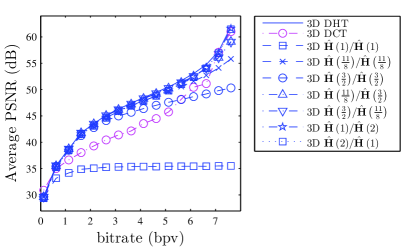
(a) PSNR

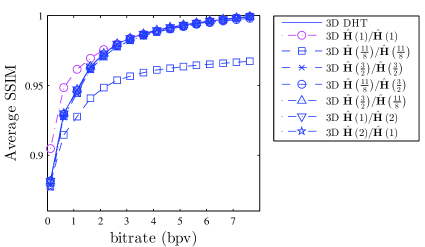
(b) SSIM

Figure 2: Average PSNR and SSIM versus bitrate of the 3D DCT, the 3D DHT, and the proposed methods for XA data.

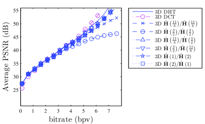
(a) PSNR

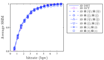
(b) SSIM

Figure 3: Average PSNR and SSIM versus bitrate of the 3D DCT, the 3D DHT, and the proposed methods for MR data.

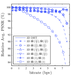
(a) PSNR

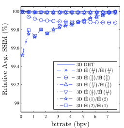
(b) SSIM

Figure 4: Relative PSNR and SSIM versus bitrate of the proposed methods related to the exact 3D DHT for XA arrays.

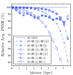
(a) PSNR

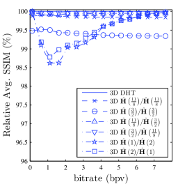
(b) SSIM

Figure 5: Relative PSNR and SSIM versus bitrate of the proposed methods related to the exact 3D DHT for MR arrays.

(a) Uncompressed XA slice

(b) 3D DCT (PSNR=43.58 dB, SSIM=0.9883)

(c) 3D DHT (PSNR=48.53 dB, SSIM=0.9902)

(d) 3D $\hat{\mathbf{H}}\left(\frac{11}{8}\right)/\hat{\mathbf{H}}\left(\frac{11}{8}\right)$ (PSNR=47.35 dB , SSIM=0.9899)

(e) 3D $\hat{\mathbf{H}}\left(\frac{3}{2}\right)/\hat{\mathbf{H}}\left(\frac{3}{2}\right)$ (PSNR= 46.02 dB, SSIM=0.9889)

(f) 3D $\hat{\mathbf{H}}\left(\frac{3}{2}\right)/\hat{\mathbf{H}}\left(\frac{11}{8}\right)$ (PSNR=48.31 dB, SSIM=0.9901)

(g) 3D $\hat{\mathbf{H}}\left(2\right)/\hat{\mathbf{H}}\left(1\right)$ (PSNR=48.04 dB, SSIM=0.9892)

Figure 6: Qualitative assessment for XA slice at 4 bpv compression rate.

We employed the proposed 3D DHT approximations in the 3D DHT-based medical image compression algorithm proposed in [80]. We selected ten X-ray angiograms (XA) and ten magnetic resonance (MR) available in [67, 73, 54, 4] with varied resolutions of $256\times 256$ or $512\times 512$ and with varied number of frames/slices. Each XA or MR data can be represented by a three-dimensional array, i.e., a third-order tensor as described in Section 3.1. Each third-order tensor was divided into smaller blocks of size $8\times 8\times 8$ and then submitted to the 3D transformation as defined in (21) and (19). Instead of considering the zigzag scheme defined in [80], in which a 2D DHT-based zigzag pattern is considered for each frame of the 3D transformed block— we have considered a truly 3D experimental zigzag pattern, which was obtained by averaging the amount of energy of the transform domain signal concentrated in each coefficient and, thus, ordering in a monotonic decreasing fashion. The transform-domain block was then applied to the zigzag scheme as explained above. For comparison, we employed the 3D DCT [75] in our simulation. Particularly for such case, we considered the usual zigzag pattern for the 3D DCT [12].

Subsequently the data was compressed at a fixed bitrate [7, 9] by preserving only a constant number $L$ of the first zig-zag coefficients which contain the most part of signal energy. In the full 3D DHT-based codec implementation, only these $L$ preserved coefficients need to be encoded by the entropy coding [70], such as Huffman coding algorithm, and then stored and/or transmitted. However, because the goal of our work is to analyze the effect of the 3D transform block and also because the entropy algorithms are lossless — do not interfere in image visual quality — we did not consider entropy coding in the present experiment. The bitrate is given in bit per voxel (bpv) and computed according to $\operatorname{bitrate}={T_{b}}/{T_{v}},$ [80], where $T_{b}$ is the size of the compressed image in total of bits and $T_{v}$ is the total of voxels. For $8\times 8\times 8$ blocks, $T_{v}=512$. The fixed number $L$ of retained coefficients determines the fixed bitrate for the present compression procedure. For instance, considering 8-bits DICOM data, to preserve 128 coefficients results in bitrate of $T_{b}/T_{v}=(8\times 128)/512=2$ bpv.

By varying the amount $L$ of coefficients retained, we ranged the bitrate for each image in the interval $\left[0.125,7.125\right]$ with step of $0.5$. The data compression procedure in our experiment for a fixed bitrate is described as follows:

1. divide the 3D data into $B$ blocks of size $8\times 8\times 8$;

2. compute the 3D transform of each $8\times 8\times 8$ block, resulting in $B$ transform-domain blocks of the same size;

3. vectorize each transform domain-block employing the 3D zigzag pattern, resulting in $B$ zigzag vector of length $8^{3}=512$;

4. Keep only the first $L$ coefficients of each zigzag vector, discarding the remaining $512-L$.

The data reconstruction procedure in our experiment for a fixed bitrate is described as follows:

1. Reconstruct $B$ 512-length vectors employing the first $L$ preserved coefficients and filling the last $512-L$ coefficients with zeros;

2. Employ the inverse 3D zigzag scheme to restore $B$ $8\times 8\times 8$ compressed transform-domain blocks;

3. Compute the inverse 3D transform of each $8\times 8\times 8$ block, resulting in $B$ image-domain recovered blocks of the same size;

4. Employ the $B$ recovered image-domain blocks of size $8\times 8\times 8$ to reconstruct the compressed 3D data.

As figure of merit measures for performance evaluation, it was utilized the peak signal-to-noise ratio (PSNR) [7, p. 9] and the structural similarity index (SSIM) [84]. The average between each metric obtained from each array was considered and weighted according to the number of blocks of each array. Our simulations showed that the discussed methods offer a similar behavior, except for the involutional method $\hat{\mathbf{H}}\left(1\right)/\hat{\mathbf{H}}\left(1\right)$. In fact, such method generates the highest deviation from diagonality, as shown in Table 2, which introduces large error when computing the inverse transformation. Thus, we excluded this case from our analysis. It is presented in Figure 2 and Figure 3 the average result for XA and MR, respectively, for all the considered methods and different bitrates. These results are also presented in Table 4 and in Table 5.

Table 4: Average PSNR (dB) and SSIM measures (respectively) for each method for different bitrates for XA datas

	Bitrate
Method	0.125	1.125	2.125	3.125	4.125	5.125	6.125	7.125
3D DHT	29.62	38.73	43.52	46.33	48.46	50.52	53.05	57.28
	.8815	.9471	.9730	.9840	.9898	.9935	.9963	.9986
3D DCT	30.89	36.64	39.30	41.36	43.56	45.77	50.40	57.04
	.9047	.9616	.9758	.9838	.9890	.9929	.9960	.9984
$\hat{\mathbf{H}}\left(\frac{11}{8}\right)/\hat{\mathbf{H}}\left(\frac{11}{8}\right)$	29.62	38.68	43.34	45.98	47.90	49.63	51.56	54.11
	.8815	.9469	.9728	.9837	.9895	.9932	.9960	.9983
$\hat{\mathbf{H}}\left(\frac{3}{2}\right)/\hat{\mathbf{H}}\left(\frac{3}{2}\right)$	29.61	38.49	42.77	44.97	46.40	47.56	48.65	49.77
	.8815	.9463	.9720	.9829	.9887	.9923	.9951	.9974
$\hat{\mathbf{H}}\left(\frac{11}{8}\right)/\hat{\mathbf{H}}\left(\frac{3}{2}\right)$	29.61	38.71	43.46	46.21	48.27	50.23	52.54	56.05
	.8814	.9470	.9729	.9838	.9897	.9934	.9962	.9985
$\hat{\mathbf{H}}\left(\frac{3}{2}\right)/\hat{\mathbf{H}}\left(\frac{11}{8}\right)$	29.62	38.71	43.46	46.22	48.28	50.23	52.53	56.05
	.8815	.9470	.9729	.9839	.9897	.9934	.9962	.9985
$\hat{\mathbf{H}}\left(1\right)/\hat{\mathbf{H}}\left(2\right)$	29.35	38.44	43.10	45.81	47.79	49.88	52.41	56.96
	.8773	.9444	.9706	.9822	.9883	.9925	.9957	.9985
$\hat{\mathbf{H}}\left(2\right)/\hat{\mathbf{H}}\left(1\right)$	29.40	38.45	43.11	45.87	47.87	49.83	52.33	56.92
	.8775	.9446	.9707	.9824	.9885	.9924	.9956	.9985

Table 5: Average PSNR (dB) and SSIM measures (respectively) for each method for different bitrates for MR datas

	Bitrate
Method	0.125	1.125	2.125	3.125	4.125	5.125	6.125	7.125
3D DHT	27.40	33.13	36.68	40.15	43.30	46.95	51.07	57.07
	.7145	.8668	.9326	.9682	.9832	.9920	.9966	.9990
3D DCT	25.67	32.23	36.70	39.72	43.06	48.03	53.04	61.09
	.6985	.8568	.9274	.9600	.9798	.9921	.9969	.9992
$\hat{\mathbf{H}}\left(\frac{11}{8}\right)/\hat{\mathbf{H}}\left(\frac{11}{8}\right)$	27.39	33.09	36.57	39.91	42.77	45.80	48.61	51.21
	.7136	.8660	.9313	.9668	.9816	.9905	.9950	.9974
$\hat{\mathbf{H}}\left(\frac{3}{2}\right)/\hat{\mathbf{H}}\left(\frac{3}{2}\right)$	27.36	32.94	36.24	39.19	41.43	43.46	44.96	45.99
	.7108	.8625	.9273	.9624	.9770	.9856	.9901	.9924
$\hat{\mathbf{H}}\left(\frac{11}{8}\right)/\hat{\mathbf{H}}\left(\frac{3}{2}\right)$	27.40	33.09	36.63	40.03	43.11	46.53	50.10	54.21
	.7142	.8662	.9320	.9676	.9826	.9915	.9961	.9985
$\hat{\mathbf{H}}\left(\frac{3}{2}\right)/\hat{\mathbf{H}}\left(\frac{11}{8}\right)$	27.40	33.12	36.64	40.07	43.12	46.55	50.12	54.25
	.7142	.8664	.9321	.9678	.9827	.9915	.9961	.9985
$\hat{\mathbf{H}}\left(1\right)/\hat{\mathbf{H}}\left(2\right)$	27.40	32.52	36.00	38.92	42.27	45.57	49.39	54.57
	.7145	.8549	.9236	.9602	.9793	.9896	.9953	.9984
$\hat{\mathbf{H}}\left(2\right)/\hat{\mathbf{H}}\left(1\right)$	27.40	32.70	36.04	39.03	42.27	45.57	49.36	54.66
	.7145	.8563	.9242	.9612	.9793	.9896	.9953	.9984

Generally, all the methods present better performance at compressing XA data than MR data. For such case, the exact 3D DHT and the proposed approximate versions present better performance than the 3D DCT in terms of PSNR for the bitrate ranging from 1 bpv to 6 bpv. For instance, at 2 bpv, the exact 3D DHT and the proposed 3D $\hat{\mathbf{H}}\left(\frac{3}{2}\right)/\hat{\mathbf{H}}\left(\frac{11}{8}\right)$ present 10.7 % and 10.6 % higher PSNR than the 3D DCT, respectively; for 6 bpv, such values are 5.2 % and 4.2%, respectively. In terms of SSIM, the 3D DCT outperform the 3D DHT and the proposed methods in the shorter range of (0 bpv, 2 bpv). For instance, at 2 bpv, the exact 3D DHT and the proposed $\hat{\mathbf{H}}\left(\frac{3}{2}\right)/\hat{\mathbf{H}}\left(\frac{11}{8}\right)$ present 0.28 % and 0.23 % lower SSIM than the 3D DCT, respectively; whereas for 6 bpv they present 0.03 % and 0.02 % higher SSIM than the 3D DCT, respectively. The results for compressing MR data are very close, with the 3D DCT presenting slightly lower PSNR values for low bitrates (¡2 bpv) and higher values for high bitrates (¿5 bpv). For example, at 1 bpv, the exact 3D DHT and the proposed $\hat{\mathbf{H}}\left(\frac{3}{2}\right)/\hat{\mathbf{H}}\left(\frac{11}{8}\right)$ present 2.8 % and 2.8 % higher PSNR than the 3D DCT, whereas, for 6 bpv, they present 3.7 % and 5.5 % lower PSNR than the 3D DCT. Generally, all the methods present a competitive performance compared to the 3D DCT. However, the exact 3D DHT shows a substantial reduction in the multiplicative complexity of of 81.8 % (see Table 3), while all the proposed 3D DHT approximations present 100 % of multiplicative complexity reduction.

Hence, we focus on comparing the proposed 3D DHT approximations with the exact 3D DHT. In Figure 4 and Figure 5, it is shown a comparison of the proposed methods with the original 3D DHT, in which it is presented the relative PSNR and SSIM compared to the exact 3D DHT-based compression.

For low bitrates ($<2$ bpv) the general performance is higher than $98\%$ in terms of PSNR and $99\%$ in terms of SSIM compared to the exact 3D DHT. For XA images, specifically, the performance of the proposed methods is higher than $99.5\%$ in terms of SSIM. The simulations suggest that all methods present better performance at compressing XA than MR images. When increasing the bitrate, the 3D DHT approximations relative PSNR decrease compared to the 3D DHT. Such percentage difference occurs because, for the exact 3D DHT, the exact inverse 3D DHT is employed to reconstruct the image and thus it achieves perfect reconstruction when the bitrate $\rightarrow 8$ bpv, which results in PSNR $\rightarrow\infty$. The proposed 3D DHT approximations, however, consider low-complexity approximate versions for the their inverse 3D transformations. Then, they do not achieve the perfect reconstruction when $\rightarrow 8$ bpv and the relative PSNR will increase for high bitrates. Such effect is not observed in the relative SSIM values because the SSIM measure ranges in the closed interval $[0,1]$. Instead, the relative SSIM increases with the bitrate. Furthermore, the absolute PSNR values show that the performance for bitrates higher than 4 bpv are higher than 40 dB for all the methods. Thus, the relative PSNR does not capture the actual perceived image quality difference. As a demonstration of such aspect, a qualitative comparison is shown in Figure 6 for a slice of an XA compressed at 4 bpv employing some of the proposed methods. The compressed images are very close to the uncompressed image and the approximate methods performances are practically indistinguishable when compared to the exact 3D DHT.

Such results show that our proposed approximate 3D DHT-based methods are as suitable to coding medical images as the exact 3D DHT-based method in [80] at a considerable lower complexity cost. Generally, the proposed approximate methods present more than $98\%$ of SSIM performance relative to the original method at a much lower computational cost.

5 Time and Memory Complexity Assessment

In the present Section, we aim at analyzing the time and memory complexity of the proposed 3D approximate transforms in a real-time processing scenario and compare them with the both traditional 3D DHT and 3D DCT. To demonstrate the appropriateness of the proposed methods in real-time embedded applications, we implemented the proposed 3D transforms in an ARM Cortex-M0+ processor. The ARM Cortex cores have been widely adopted in low-power and real-time embedded applications, such as internet of things devices [41, 89, 65].

We employed the Raspberry Pi Pico board [81], which is equipped with the recently introduced RP2040 microcontroller. The RP2040 is a low cost and low power chip designed by Raspberry Pi, presenting a dual-core ARM Cortex-M0+ processor with 264KB internal random access memory. In addition, we considered the C language with the Software Development Kit (SDK) libraries for C/C++ [82] in our code implementation.

Following the mathematical development of Section 3, we implemented the 3D transforms by means of several 1D algorithms for each vector in each dimension. Such procedure is employed to compute the 3D SDHT, the proposed 3D SDHT aproximations and the 3D DCT. To compute the 1D algorithms for the DHT and the proposed approximate versions, the flow-graph of Figure 1 is implemented. For the DCT case, we considered the Loeffler algorithm [56], which is optimum in terms of multiplicative complexity of the DCT [40]. The procedure is summarized as follows:

1. compute $64$ 1D transforms of each row (1st dimension);

2. transpose the array by shifting dimensions, i.e., $n_{1}\times n_{2}\times n_{3}$ turns to $n_{2}\times n_{3}\times n_{1}$;

3. compute $64$ 1D transforms of each row of the transposed array (2nd dimension);

4. transpose the array by shifting dimensions, i.e., $n_{2}\times n_{3}\times n_{1}$ turns to $n_{3}\times n_{1}\times n_{2}$;

5. compute $64$ 1D transforms of each row of the transposed array (3rd dimension);

6. transpose the array back to its original position by shifting dimensions, i.e., $n_{3}\times n_{1}\times n_{2}$ turns to $n_{1}\times n_{2}\times n_{3}$.

Next, it is required to employ the 3D SDHT (or an approximate version) to compute the 3D DHT (or an approximate version) according to (16) and (19). Such operation requires only additions, as described in Section 3.3 and it is implemented with a triple “for” loop. Notice that the 3D DCT does not require such procedure because it is already a separable transform.

Our implementation is performed sequentially in a single core and considers $8\times 8\times 8$ input arrays of 32-bits integers. For the exact 3D DHT and the 3D DCT cases, the multiplications by the irrational quantities are performed via floating point multiplication, i.e., the input integer coefficient is converted to floating point representation (via type casting), multiplied by the irrational constant, and then converted back to integer. On the other hand, for the proposed approximate 3D DHTs, the multiplications by the dyadic rationals are realized by integers bitshifts and additions only, according to Table 1. Thus, the proposed methods do not require any multiplication operation at all, as presented in Section 3.3.

We compute the 3D transforms of 8,192 blocks of size $8\times 8\times 8$, randomly generated. For instance, such number of blocks is equivalent to a full DICOM data of size $265\times 256\times 64$. Our goal is to analyze the elapsed time and the memory usage for each 3D transform employed in the present experiment. The time elapsed was obtained employing the RP2040 timestamp function available in the SDK library. The results are shown in Table 6. We repeated the above experiment fifty times and considered the average time elapsed.

It can be observed that the proposed methods present a substantial reduction in terms of execution time compared to both the 3D DCT and the 3D DHT. Particularly, the proposed 3D method based on $\hat{\mathbf{H}}\left(1\right)$ presented the fastest execution of 3200 ms, which corresponds to percentage reductions compared to the 3D DCT and 3D DHT of 91.22 % and 72.53 %, respectively. Such result is expected since such 3D method presents the lowest arithmetic complexity, as shown in Table 3. Generally, all the proposed 3D methods present significant reduction in execution time, with percentage reduction compared to the 3D DCT and 3D DHT of $\sim$90 % and $\sim$70%. Such results are consequence of the fact the proposed methods present null multiplicative complexity.

Table 6: Execution time for each 3D method and the respective percentage reduction compared to the 3D DCT execution time employing the RP2040 microcontroller

Method	Elapsed time (ms)	reduction to 3D DCT	reduction to 3D DHT
3D DCT row-column on [56]	36457	—	—
3D DHT row-column on Figure 1	11650	68.04 %	—
Proposed 3D method based on $\hat{\mathbf{H}}\left(1\right)$	3200	91.22 %	72.53 %
Proposed 3D method based on $\hat{\mathbf{H}}\left(\frac{11}{8}\right)$	3637	90.02 %	68.78 %
Proposed 3D method based on $\hat{\mathbf{H}}\left(\frac{3}{2}\right)$	3513	90.36 %	69.84 %
Proposed 3D method based on $\hat{\mathbf{H}}\left(2\right)$	3521	90.34 %	69.77 %

For the memory usage, we analyzed the memory usage observing the compiler output Executable and Linkable Format (ELF) file [2]. We considered the .text segment, which is a measure of the code length [3, p. 64], and the the .data and the .bss segments, which hold the initialized and uninitialized data, respectively, and measure together the statically allocated memory [3, p. 62] — we did not employ dynamic allocation in the present experiment. The memory usage for each method is shown in Table 7. In general, all the methods present the same usage for statically allocated memory and minor difference in code length. Such result is expected since the proposed methods address the reduction in arithmetic complexity, which results in a faster execution but preserve the same structure in terms of transform and vector lengths.

Table 7: Memory usage for each 3D method employing the RP2040 microcontroller

	Memory usage (bytes)
Method	.text	.data + .bss
3D DCT row-column on [56]	30160	1072 + 3428 = 4500
3D DHT row-column on Figure 1	29904	1072 + 3428 = 4500
Proposed 3D method based on $\hat{\mathbf{H}}\left(1\right)$	29472	1072 + 3428 = 4500
Proposed 3D method based on $\hat{\mathbf{H}}\left(\frac{11}{8}\right)$	29416	1072 + 3428 = 4500
Proposed 3D method based on $\hat{\mathbf{H}}\left(\frac{3}{2}\right)$	29376	1072 + 3428 = 4500
Proposed 3D method based on $\hat{\mathbf{H}}\left(2\right)$	29376	1072 + 3428 = 4500

6 Conclusion

In the present work, we proposed a mathematical formulation for approximating the 3D DHT based on tensor formalism. A parametric exhaustive search for deriving approximations for the DHT matrix was performed. A set of quasi-orthogonal approximate DHT matrices was presented. Such matrices are optimized according to performance, arithmetic complexity and quasi-orthogonality measures.

A collection of $8\times 8\times 8$ multiplierless 3D DHT approximations based on the derived approximate matrices was proposed. The derived 3D transforms were applied to the 3D DHT-based DICOM medical image coding scheme in [80]. We also included the 3D DCT for comparison. The results showed very close performance ($>98\%$ in terms of SSIM relative to the original method) at a considerable lower computational cost ($100\%$ multiplicative complexity reduction). The proposed methods are realistic low-complexity coding algorithms that can be employed in medical image compression, transmission and storage systems presenting rigorous energy and hardware resources constraints.

Furthermore, we have implemented the proposed methods as well as the classical 3D DCT and 3D DHT in an ARM Cortex-M0+ processor employing the recently introduced Raspberry Pi Pico board. We analyzed the execution time and memory consumption. The results show a noticeable execution time reduction of $\sim 90\%$ and $\sim 70\%$ compared to the 3D DCT and the 3D DHT, respectively, whereas the memory usage is not significantly affected. Thus, we conclude that the main advantage of the proposed methods is the lower arithmetic cost which allow lower execution time at minor degradation in performance, which suggests a favorable trade-off.

As limitations of the present work, we mention:

1. the quasi-orthogonality property introduces error in the 3D inverse computation. This error is negligible for low bitrates. It tends, however, to be more prominent in terms of relative PSNR at high bitrates compared to the exact 3D DHT; this increase is not observed for the SSIM metric, which suggests that the error is almost unnoticeable for the human vision;

2. the proposed methods do not reduce the memory usage. This property is expected since the transforms are designed to have reduced arithmetic complexity, but they still present the same input and output sizes and the same transform lengths.

For future work, we suggest:

1. implementing dedicate circuits in FPGA and ASICs for computing the proposed 3D DHT in order to evaluate the components and area reduction;

2. evaluating how well the proposed methods perform to compress natural videos and other 3D image data;

3. expanding the current approach for higher lengths 3D transforms, such as transforms of sizes $16\times 16\times 16$ and $32\times 32\times 32$.

4. investigating the relation of the DHT and its approximate versions with the graph Fourier transform and possible applications in wireless sensor networks;

5. investigating higher dimension DHT approximations such as 4D DHT and 5D DHT and possible applications at compressing multidimensional image data such as lightfield data.

References

- [1] N. Ahmed and K. R. Rao, Orthogonal Transforms for Digital Signal Processing, Springer, 1975.
- [2] ARM Developer, ARM ELF specification.
- [3] AT&T, The Santa CruzOperation Inc., System V Application Binary Interface, 4.1 ed., 1997.
- [4] S. Barré, Medical imaging samples.
- [5] F. M. Bayer and R. J. Cintra, DCT-like transform for image compression requires 14 additions only, Electronics Letters, 48 (2012), pp. 919–921.
- [6] D. S. Bernstein, Matrix Mathematics: Theory, Facts, and Formulas, Princeton University Press, 2009.
- [7] V. Bhaskaran and K. Konstantinides, Image and Video Compression Standards, Kluwer Academic Publishers, 1997.
- [8] R. E. Blahut, Fast Algorithms for Signal Processing, Cambridge University Press, 2010.
- [9] S. Bouguezel, M. O. Ahmad, and M. N. S. Swamy, Low-complexity 88 transform for image compression, Electronics Letters, 44 (2008), pp. 1249–1250.
- [10] , Binary discrete cosine and Hartley transforms, IEEE Transactions on Circuits and Systems I: Regular Papers, 60 (2013), pp. 989–1002.
- [11] S. Boussakta, O. H. Alshibami, and M. Y. Aziz, Radix- algorithm for the 3-D discrete Hartley transform, IEEE Transactions on Signal Processing, 49 (2001), pp. 3145–3156.
- [12] N. Bozinović and J. Konrad, Scan order and quantization for 3D-DCT coding, in Proceedings of SPIE Visual Communications and Image Processing, vol. 5150, 2003, p. 1205.
- [13] , Motion analysis in 3D DCT domain and its application to video coding, Signal Processing: Image Communication, 20 (2005), pp. 510–528.
- [14] R. N. Bracewell, Discrete Hartley transform, Journal of the Optical Society of America, 73 (1983), pp. 1832–1835.
- [15] R. N. Bracewell, O. Buneman, H. Hao, and J. Villasenor, Fast two-dimensional Hartley transform, Proceedings of the IEEE, 74 (1986), pp. 1282–1283.
- [16] V. Britanak, P. Yip, and K. R. Rao, Discrete Cosine and Sine Transforms, Academic Press, 2007.
- [17] Y.-L. Chan and W.-C. Siu, Variable temporal-length 3-D discrete cosine transform coding, IEEE Transactions on Image Processing, 6 (1997), pp. 758–763.
- [18] J.-T. Chien and Y.-T. Bao, Tensor-factorized neural networks, IEEE Transactions on Neural Networks and Learning Systems, 29 (2018), pp. 1998–2011.
- [19] D. F. Chiper, A novel VLSI DHT algorithm for a highly modular and parallel architecture, IEEE Transactions on Circuits and Systems II: Express Briefs, 60 (2013), pp. 282–286.
- [20] R. J. Cintra, An integer approximation method for discrete sinusoidal transforms, Circuits, Systems, and Signal Processing, 30 (2011), pp. 1481–1501.
- [21] R. J. Cintra and F. M. Bayer, A DCT approximation for image compression, IEEE Signal Processing Letters, 18 (2011), pp. 579–582.
- [22] R. J. Cintra, F. M. Bayer, Y. Pauchard, and A. Madanayake, Low-Complexity DCT Approximations for Biomedical Signal Processing in Big Data, CRC Press, 1 ed., 2018, p. 624.
- [23] R. J. Cintra, F. M. Bayer, and C. J. Tablada, Low-complexity 8-point DCT approximations based on integer functions, Signal Processing, 99 (2014), pp. 201–214.
- [24] V. A. Coutinho, R. J. Cintra, and F. M. Bayer, Low-complexity multidimensional DCT approximations for high-order tensor data decorrelation, IEEE Transactions on Image Processing, 26 (2017), pp. 2296–2310.
- [25] T. L. T. da Silveira, F. M. Bayer, R. J. Cintra, S. Kulasekera, A. Madanayake, and A. J. Kozakevicius, An orthogonal 16-point approximate DCT for image and video compression, Multidimensional Systems and Signal Processing, 27 (2016), pp. 87–104.
- [26] L. De Lathauwer and B. De Moor, From matrix to tensor: Multilinear algebra and signal processing, in Institute of Mathematics and Its Applications Conference Series, vol. 67, Citeseer, 1998, pp. 1–16.
- [27] L. De Lathauwer, B. De Moor, and J. Vandewalle, On the best rank-1 and rank-() approximation of higher-order tensors, SIAM Journal on Matrix Analysis and Applications, 21 (2000), pp. 1324–1342.
- [28] M. R. Descour, A. Karkkainen, J. D. Rogers, C. Liang, R. S. Weinstein, J. T. Rantala, B. Kilic, E. Madenci, R. R. Richards-Kortum, E. V. Anslyn, et al., Toward the development of miniaturized imaging systems for detection of pre-cancer, IEEE Journal of Quantum Electronics, 38 (2002), pp. 122–130.
- [29] M. Dousty, S. Daneshvar, and R. C. Sotero, Multifocus image fusion via the Hartley transform, in Canadian Conference on Electrical and Computer Engineering (CCECE), IEEE, 2016, pp. 1–5.
- [30] P. Duhamel and M. Vetterli, Fast Fourier transforms: a tutorial review and a state of the art, Signal Processing, 19 (1990), pp. 259–299.
- [31] I. Duleba, Hartley transform in compression of medical ultrasonic images, in Proceedings of the International Conference on Image Analysis and Processing, IEEE, 1999, pp. 722–727.
- [32] E. Feig and S. Winograd, Fast algorithms for the discrete cosine transform, IEEE Transactions on Signal Processing, 40 (1992), pp. 2174–2193.
- [33] Y. Gao, Y. Zheng, S. Diao, W.-D. Toh, C.-W. Ang, M. Je, and C.-H. Heng, Low-power ultrawideband wireless telemetry transceiver for medical sensor applications, IEEE Transactions on Biomedical Engineering, 58 (2011), pp. 768–772.
- [34] O. N. Gerek and A. E. Çetin, A 2-D orientation-adaptive prediction filter in lifting structures for image coding, IEEE Transactions on Image Processing, 15 (2006), pp. 106–111.
- [35] R. C. Gonzalez and R. Woods, Digital Image Processing, Prentice Hall, 2001.
- [36] A. M. Grigoryan, A novel algorithm for computing the 1-D discrete Hartley transform, IEEE Signal Processing Letters, 11 (2004), pp. 156–159.
- [37] J.-I. Guo, An efficient design for one-dimensional discrete Hartley transform using parallel additions, IEEE Transactions on Signal Processing, 48 (2000), pp. 2806–2813.
- [38] H. Hao and R. N. Bracewell, A three-dimensional DFT algorithm using the fast Hartley transform, Proceedings of the IEEE, 75 (1987), pp. 264–266.
- [39] T. I. Haweel, A new square wave transform based on the DCT, Signal Processing, 82 (2001), pp. 2309–2319.
- [40] M. T. Heideman, Multiplicative Complexity, Convolution, and the DFT, Signal Processing and Digital Filtering, Springer-Verlag, 1988.
- [41] S. Höppner, H. Eisenreich, D. Walter, U. Steeb, A. S. C. Dmello, R. Sinkwitz, H. Bauer, A. Oefelein, F. Schraut, J. Schreiter, et al., How to achieve world-leading energy efficiency using 22FDX with adaptive body biasing on an ARM cortex-M4 IoT SoC, in ESSDERC 2019-49th European Solid-State Device Research Conference (ESSDERC), IEEE, 2019, pp. 66–69.
- [42] M. F. Hossain, M. R. Alsharif, and K. Yamashita, Medical image enhancement based on nonlinear technique and logarithmic transform coefficient histogram matching, in IEEE/ICME International Conference on Complex Medical Engineering, IEEE, 2010, pp. 58–62.
- [43] H. S. Hou, The fast Hartley transform algorithm, IEEE Transactions on Computers, 100 (1987), pp. 147–156.
- [44] J. A. Jacob and N. S. Kumar, FPGA implementation of optimal 3D-integer DCT structure for video compression, The Scientific World Journal, 2015 (2015).
- [45] L. Jiang, H. Shu, J. Wu, L. Wang, and L. Senhadji, A novel split-radix fast algorithm for 2-D discrete Hartley transform, IEEE Transactions on Circuits and Systems I: Regular Papers, 57 (2010), pp. 911–924.
- [46] S. Kim and W. Sung, A floating-point to fixed-point assembly program translator for the TMS 320C25, IEEE Transactions on Circuits and Systems II: Analog and Digital Signal Processing, 41 (1994), pp. 730 – 739.
- [47] N. Kouadria, N. Doghmane, D. Messadeg, and S. Harize, Low complexity DCT for image compression in wireless visual sensor networks, Electronics Letters, 49 (2013), pp. 1531–1532.
- [48] S. Kulasekera, A. Madanayake, D. Suarez, R. J. Cintra, and F. M. Bayer, Multi-beam receiver apertures using multiplierless 8-point approximate DFT, in Radar Conference (RadarCon), IEEE, 2015, pp. 1244–1249.
- [49] M.-H. Lee, CSD filter design for VLSI implementation of GA-VSB receiver, IEEE Transactions on Consumer Electronics, 43 (1997), pp. 197–206.
- [50] K. Lengwehasatit and A. Ortega, Scalable variable complexity approximate forward DCT, IEEE Transactions on Circuits and Systems for Video Technology, 14 (2004), pp. 1236–1248.
- [51] L. Li and Z. Hou, Multiview video compression with 3D-DCT, in ITI 5th International Conference on Information and Communications Technology, 2007, pp. 59–61.
- [52] X. Li, A. Dick, C. Shen, A. van den Hengel, and H. Wang, Incremental learning of 3D-DCT compact representations for robust visual tracking, IEEE Transactions on Pattern Analysis and Machine Intelligence, 35 (2013), pp. 863–881.
- [53] J. Liang and T. D. Tran, Fast multiplierless approximation of the DCT with the lifting scheme, IEEE Transactions on Signal Processing, 49 (2001), pp. 3032–3044.
- [54] W. R. Lionheart, An MRI DICOM data set of the head of a normal male human aged 52.
- [55] Z. Liu, J. Dai, X. Sun, and S. Liu, Color image encryption by using the rotation of color vector in Hartley transform domains, Optics and Lasers in Engineering, 48 (2010), pp. 800–805.
- [56] C. Loeffler, A. Ligtenberg, and G. S. Moschytz, Practical fast 1-D DCT algorithms with 11 multiplications, ICASSP International Conference on Acoustics, Speech, and Signal Processing, 2 (1989), pp. 988–991.
- [57] A. Madanayake, R. J. Cintra, V. Dimitrov, F. M. Bayer, K. A. Wahid, S. Kulasekera, A. Edirisuriya, U. Potluri, S. Madishetty, and N. Rajapaksha, Low-power VLSI architectures for DCT/DWT: precision vs approximation for HD video, biomedical, and smart antenna applications, IEEE Circuits and Systems Magazine, 15 (2015), pp. 25–47.
- [58] J. K. Mandal and S. K. Ghosal, Separable discrete Hartley transform based invisible watermarking for color image authentication (SDHTIWCIA), in Advances in Computing and Information Technology, Springer, 2013, pp. 767–776.
- [59] P. K. Meher, T. Srikanthan, and J. C. Patra, Scalable and modular memory-based systolic architectures for discrete Hartley transform, IEEE Transactions on Circuits and Systems I: Regular Papers, 53 (2006), pp. 1065–1077.
- [60] A. Mulla, J. Baviskar, A. Baviskar, and C. Warty, Image compression scheme based on zig-zag 3D-DCT and LDPC coding, in International Conference on Advances in Computing, Communications and Informatics (ICACCI), 2014, pp. 2380–2384.
- [61] K. C. Narendra and S. Satyanarayana, Hartley transform based correlation filters for face recognition, in International Conference on Signal Processing and Communications (SPCOM), IEEE, 2016, pp. 1–5.
- [62] B. P. Nguyen, C.-K. Chui, S.-H. Ong, and S. Chang, An efficient compression scheme for 4-D medical images using hierarchical vector quantization and motion compensation, Computers in Biology and Medicine, 41 (2011), pp. 843–856.
- [63] P. A. Oliveira, R. J. Cintra, F. M. Bayer, S. Kulasekera, and A. Madanayake, Low-complexity image and video coding based on an approximate discrete Tchebichef transform, IEEE Transactions on Circuits and Systems for Video Technology, 27 (2017), pp. 1066–1076.
- [64] P. A. M. Oliveira, R. S. Oliveira, R. J. Cintra, F. M. Bayer, and A. Madanayake, JPEG quantisation requires bit-shifts only, Electronics Letters, 53 (2017), pp. 588–590.
- [65] T. Onuki, W. Uesugi, A. Isobe, Y. Ando, S. Okamoto, K. Kato, T. R. Yew, J. Wu, C. C. Shuai, S. H. Wu, et al., Embedded memory and ARM cortex-M0 core using 60-nm C-axis aligned crystalline indium–gallium–zinc oxide FET integrated with 65-nm Si CMOS, IEEE Journal of Solid-State Circuits, 52 (2017), pp. 925–932.
- [66] A. V. Oppenheim and R. W. Schafer, Discrete-time Signal Processing, Pearson Higher Education, 3rd ed., 2010.
- [67] OsiriX DICOM, OsiriX DICOM image sample sets.
- [68] J. Papitha, G. M. Nancy, and D. Nedumaran, Compression techniques on MR image—a comparative study, in International Conference on Communications and Signal Processing (ICCSP), IEEE, 2013, pp. 367–371.
- [69] Y. Pauchard, R. J. Cintra, A. Madanayake, and F. M. Bayer, Fast computation of residual complexity image similarity metric using low-complexity transforms, IET Image Processing, 9 (2015), pp. 699–708.
- [70] K. R. Rao and P. Yip, The Transform and Data Compression Handbook, CRC Press LLC, 2001.
- [71] , Discrete Cosine Transform: Algorithms, Advantages, Applications, Academic Press, San Diego, CA, 2014.
- [72] M. Rizkalla, P. M. Ei-Sharkawy Salama, and B. Dukel, Implementation of floating point fast discrete cosine transform, The 45th Midwest Symposium on Circuits and Systems (MWSCAS), 2 (2002), pp. II–17 – II–20.
- [73] Rubo Medical Imaging, Rubo medical imaging dataset.
- [74] S. Sawant and D. A. Adjeroh, Balanced multiple description coding for 3D DCT video, IEEE Transactions on Broadcasting, 57 (2011), pp. 765–776.
- [75] M. Servais and G. de Jager, Video compression using the three dimensional discrete cosine transform (3D-DCT), in Proceedings of the 1997 South African Symposium on Communications and Signal Processing (COMSIG), IEEE, 1997, pp. 27–32.
- [76] T. Song and H. Li, Local polar DCT features for image description, IEEE Signal Processing Letters, 20 (2013), pp. 59–62.
- [77] H. Sorensen, D. Jones, C. Burrus, and M. Heideman, On computing the discrete Hartley transform, IEEE Transactions on Acoustics, Speech, and Signal Processing, 33 (1985), pp. 1231–1238.
- [78] D. Suarez, R. J. Cintra, F. M. Bayer, A. Sengupta, S. Kulasekera, and A. Madanayake, Multi-beam RF aperture using multiplierless FFT approximation, Electronics Letters, 50 (2014), pp. 1788–1790.
- [79] R. S. Sunder, C. Eswaran, and N. Sriraam, Performance evaluation of 3-D transforms for medical image compression, in Proceedings of the International Conference on Electro Information Technology, IEEE, 2005, pp. 6–pp.
- [80] R. S. Sunder, C. Eswaran, and N. Sriraam, Medical image compression using 3-D Hartley transform, Computers in Biology and Medicine, 36 (2006), pp. 958–973.
- [81] The Raspberry Pi Foundation, Raspberry Pi Pico.
- [82] , Raspberry Pi Pico Software Development Kit (SDK).
- [83] Y. Voronenko and M. Puschel, Algebraic signal processing theory: Cooley–Tukey type algorithms for real DFTs, IEEE Transactions on Signal Processing, 57 (2009), pp. 205–222.
- [84] Z. Wang, A. C. Bovik, H. R. Sheikh, and E. P. Simoncelli, Image quality assessment: from error visibility to structural similarity, IEEE Transactions on Image Processing, 13 (2004), pp. 600–612.
- [85] A. B. Watson and A. Poirson, Separable two-dimensional discrete Hartley transform, Journal of the Optical Society of America A, 3 (1986), pp. 2001–2004.
- [86] M. Xue, A. Mian, W. Liu, and L. Li, Automatic 4D facial expression recognition using DCT features, in Winter Conference on Applications of Computer Vision, IEEE, 2015, pp. 199–206.
- [87] A. Yakovlev, S. Kim, and A. Poon, Implantable biomedical devices: Wireless powering and communication, IEEE Communications Magazine, 50 (2012).
- [88] R. Zaharia, A. Aggoun, and M. McCormick, Adaptive 3D-DCT compression algorithm for continuous parallax 3D integral imaging, Signal Processing: Image Communication, 17 (2002), pp. 231–242.
- [89] Y. Zhang, L. Xu, Q. Dong, J. Wang, D. Blaauw, and D. Sylvester, Recryptor: A reconfigurable cryptographic cortex-M0 processor with in-memory and near-memory computing for IoT security, IEEE Journal of Solid-State Circuits, 53 (2018), pp. 995–1005.