A Class of Low-Complexity DCT-like Transforms for Image and Video Coding

The discrete cosine transform (DCT) is a relevant tool in signal processing applications, mainly known for its good decorrelation properties. Current image and video coding standards—such as JPEG and HEVC—adopt the DCT as a fundamental building block for compression. Recent works have introduced low-complexity approximations for the DCT, which become paramount in applications demanding real-time computation and low-power consumption. The design of DCT approximations involves a trade-off between computational complexity and performance. This paper introduces a new multiparametric transform class encompassing the round-off DCT (RDCT) and the modified RDCT (MRDCT), two relevant multiplierless 8-point approximate DCTs. The associated fast algorithm is provided. Four novel orthogonal low-complexity 8-point DCT approximations are obtained by solving a multicriteria optimization problem. The optimal 8-point transforms are scaled to lengths 16 and 32 while keeping the arithmetic complexity low. The proposed methods are assessed by proximity and coding measures with respect to the exact DCT. Image and video coding experiments hardware realization are performed. The novel transforms perform close to or outperform the current state-of-the-art DCT approximations.

Keywords
DCT approximation, low-complexity transforms, image and video coding

1 Introduction

Discrete transforms play a central role in digital signal processing tasks, such as analysis, filtering, and coding [51]. Remarkable transforms include the discrete Hartley transform, the Haar transform, the discrete Fourier transform, the Karhunen-Loève transform (KLT), and the discrete sine and cosine transforms [16, 58, 2]. In the context of signal encoding, the KLT holds optimal decorrelation properties [16] though being data-dependent [61] and, thus, computationally complex and expensive [61, 1]. Nonetheless, the discrete cosine transform (DCT), which is signal-independent, performs close to optimal when applied to a high correlated first-order Markov random process [31, 39]. Natural images belong to this particular statistical class [55], which makes efficient implementations of the DCT to be widely adopted in current image and video coding standards [45].

Block transformation, fast algorithms, and approximate computing are some of the approaches for reducing the computational cost of the DCT applications [16]. Traditional image and video coding standards—such as the Joint Photography Experts Group (JPEG) [64] and the High Efficiency Video Coding (HEVC) [59]—operate in a block-based fashion, where the input signal is firstly segmented into disjoint blocks and then transformed accordingly [66]. For instance, JPEG uses the 8-point DCT [64], whereas HEVC adopts transforms of length 4, 8, 16, and 32 for taking advantage of highly-correlated image parts of different sizes [54]. Applying the DCT on an image block may result in few localized, meaningful coefficients that are further quantized. The low-frequency non-separable transform (LFNST) [38] explicitly discards high-frequency coefficients before quantization for reducing memory usage and computation in the new Versatile Video Coding (VVC) [69]. Because of its relevance on image compression, several fast algorithms for the DCT calculation are reported in literature [18, 41, 39, 31, 63, 42]. These approaches commonly explore sparse matrix factorizations [18, 41], recursiveness [39, 31], and relationships with other transforms [63, 42]. These efforts resulted in algorithms that attain the theoretical minimum multiplicative complexity [29], being nowadays a quite mature research area.

Even considering these algorithms, the DCT-based transformation requires irrational quantities to be computed and stored, increasing the complexity of both encoders and decoders [45]. Irrational quantities are often represented as floating-point in modern computers [33], however, such floating-point dependence may jeopardize the application of the DCT in very low-power scenarios [27, 24]. Internet of Things (IoT) applications [3, 67] often employ low-power wide area networks (LPWANs) for video transmission. Most IoT devices are designed at the lowest hardware cost, smaller hardware size, and the lowest battery consumption possible, and the LPWANs present narrow bandwidths. Low-complexity data compression mechanisms become crucial in such cases. In the past few years, several works proposed low-complexity DCT approximations, mostly of length 8, capable of compromising between arithmetic complexity and coding efficiency [19, 5, 28, 13, 60, 10, 11, 14, 40, 12, 48]. Most of these linear transformation matrices have entries defined over the set $\mathcal{C}=\{0,\pm\frac{1}{2},\pm 1,\pm 2\}$, and, thus, can be implemented using only addition and bit-shifting operations [19, 13, 21]. Indeed, multiplication-free transforms are remarkable for reducing circuitry, chip area, and power consumption in hardware implementations [53, 35].

Prominent 8-point approximate DCTs include the signed DCT [28], the series of transforms proposed by Bouguezel-Ahmad-Swamy [13, 10, 11, 14, 12], the Lengwehasatit-Ortega transform [40], the angle similarity-based DCT approximation [48], the classes of transforms from [60] and [17], and, especially, the round-off DCT (RDCT) [19], and the modified RDCT (MRDCT) [5]. On the one hand, the RDCT outperforms the current state-of-the-art low-complexity DCT approximations in terms of energy compaction properties [35, 47] at the expense of 22 additions. On the other hand, the MRDCT is a very low-complexity DCT-like transform that requires only 14 additions, the lowest arithmetic cost among the meaningful approximate DCTs archived in literature [21, 23]. Other very low-complexity approaches include the 14-additions transform from [53] and the pruned MRDCT [21], but they perform poorer in image coding applications.

Overall, the current literature still lacks unifying schemes that encompass known low-complexity DCT approximations. Some authors, although, found that such formalizations might be useful for exploring structural properties and proposing novel, more powerful, transforms [60, 17, 20]. Most of the classic related works focus on proposing 8-point DCT approximations only. Nowadays, however, there is a need for larger transforms for coping with high-resolution data [59, 35]. Some works proposed 16-point transforms [6, 22, 23], but none focused on larger blocklengths. To the best of our knowledge, there are only a few works exploring scalable approximate DCTs [12, 14, 35, 48, 17].

Our contributions are the following. First, we introduce a new class of low-complexity DCT-like transforms using a multiparametric formulation that encompasses the RDCT and the MRDCT as particular cases. Our formalism explores the underlying search space aiming at transforms with both low-complexity and good energy compaction properties. Second, we search for optimal transforms through a multicriteria optimization procedure and introduce new orthogonal 8-point approximate DCTs. Third, we use a scaling method [35] for proposing novel 16- and 32-point DCT approximations based on the optimal 8-point transforms, which are applicable to high-resolution image and video coding. The best performing transforms are assessed through image, video, and hardware experiments, and then compared with state-of-the-art methods. The results indicate their potential applicability in low-power or real-time video transmission scenarios [27, 24, 53].

The rest of this paper is organized as follows. Section 2 introduces our multiparametric 8-point DCT formulation as well as its underlying arithmetic complexity and fast algorithm. Section 3 presents a constrained multicriteria optimization procedure for acting over the search space associated with the proposed formalism and introduces the optimal 8-point DCT-like transforms. Section 4 details the adopted approach for transform scaling and presents the resulting 16- and 32-point DCT approximations. In Section 5, the optimal 8-point approximate DCTs, and their scaled versions are submitted to image and video coding experiments in which quality degradation is measured. Section 6 presents a hardware implementation of the optimal 8-point approximate DCTs. A comprehensive comparison with competing methods is presented in and in Sections 3, 4, 5, and 6. Section 7 concludes this work.

2 Multiparametric approximate DCTs

Good approximations for the 8-point DCT matrix can be obtained according to a judicious substitution of the 64 matrix entries by values in $\mathcal{C}=\{0,\pm\frac{1}{2},\pm 1,\pm 2\}$ while optimizing a given figure of merit. Because the search space increases quadratically, approaching such optimization problem by exhaustive computational search has proven to be of limited practicality in contemporary computers [52]; thus motivating alternative methods for obtaining approximate matrices. A successful approach consists of limiting the search space according to constraints from a particular parametrization of the DCT matrix entries [13, 60, 17, 20].

In [13], a class of low-complexity transforms was introduced based on a single free parameter. A parametrization of the real entries of the Feig-Winograd fast algorithm [25] was proposed in [60], leading to a multiparametric class that encompasses several DCT approximations. At the same vein, the Loeffler fast algorithm [41] was given a parametrization in [20] which furnished DCT approximations. The methodology in [17] focused on deriving DCT approximations based on a unifying mathematical treatment for the suit of approximate transforms introduced by Bouguezel, Ahmad, and Swamy [13, 10, 11, 14, 12].

2.1 Proposed Class of Low-complexity Transforms

We separate transformation matrices of the RDCT [19] and the MRDCT [5] and submit them to a parametrization of its entries. These approximations were selected because of their relevance to the approximate DCT computation literature in terms of combining high coding performance and very low arithmetic complexity, respectively. Both are 8-point orthogonal transforms whose associated low-complexity, integer transformation matrix entries are in the set $\{0,\pm 1\}\subset\mathcal{C}$, thus demanding addition operations only. Our multiparametric formulation accounts for element changes in MRDCT matrix with respect to the RDCT. The proposed multiparametric low-complexity transformation matrix is given by

$$\mathbf{T(a)}=\begin{bmatrix}1&1&1&1&1&1&1&1\\ 1&a_{1}&a_{2}&0&0&-a_{2}&-a_{1}&-1\\ 1&0&0&-1&-1&0&0&1\\ a_{3}&0&-1&-a_{4}&a_{4}&1&0&-a_{3}\\ 1&-1&-1&1&1&-1&-1&1\\ a_{5}&-1&0&a_{6}&-a_{6}&0&1&-a_{5}\\ 0&-1&1&0&0&1&-1&0\\ 0&-a_{7}&a_{8}&-1&1&-a_{8}&a_{7}&0\end{bmatrix},$$ (1)

where $\mathbf{a}=[a_{1}\enskip a_{2}\enskip a_{3}\enskip a_{4}\enskip a_{5}\enskip a_{6}\enskip a_{7}\enskip a_{8}]^{\top}$ is the parameter vector. In order to keep the complexity low and the search space withing the available computation capabilities, we focus on the case that the elements of $\mathbf{a}$ are in the set $\mathcal{C}=\{0,\pm\frac{1}{2},\pm 1,\pm 2\}$. This set extends the low-complexity sets considered in [19] and [5] by the inclusion of $\{\pm\frac{1}{2},\pm 2\}$. Thus, the resulting parametrized matrices might require bit-shifting operations. The proposed multiparametric transform class in (1) includes $7^{8}=5,764,801$ different transformation matrices; constituting the search space in which we aim at finding suitable transforms for image and video coding.

2.2 Fast Algorithm and Arithmetic Complexity

The arithmetic complexity provides a fair, unbiased assessment of the cost of applying a transform, and it is independent of the available technology [8, 50]. Directly multiplying the matrix $\mathbf{T(a)}$ by a vector is as low as 24 additions (for $\mathbf{a}$ is the null 8-point vector), increasing according to the particular choices of the parameter vector $\mathbf{a}$. The computational cost of the proposed multiparametric transform $\mathbf{T(a)}$ can be dramatically reduced by means of the following sparse factorization:

$$\mathbf{T(a)}=\mathbf{P}\cdot\mathbf{K(a)}\cdot\mathbf{A_{2}}\cdot\mathbf{A_{1}},$$ (2)

where

$$\mathbf{A_{1}}=\begin{bmatrix}\mathbf{I}_{4}&\mathrm{bar}{\mathbf{I}}_{4}\\ \mathrm{bar}{\mathbf{I}}_{4}&-\mathbf{I}_{4}\end{bmatrix},\quad\mathbf{A_{2}}={\rm diag}\left(\begin{bmatrix}\mathbf{I}_{2}&\mathrm{bar}{\mathbf{I}}_{2}\\ \mathrm{bar}{\mathbf{I}}_{2}&-\mathbf{I}_{2}\end{bmatrix},\mathbf{I}_{4}\right),$$ (3)

$$\mathbf{K(a)}={\rm diag}\left(\begin{bmatrix}1&1\\ 1&-1\end{bmatrix},-1,1,\begin{bmatrix}-a_{4}&-1&0&a_{3}\\ a_{6}&0&-1&a_{5}\\ 0&a_{2}&a_{1}&1\\ -1&a_{8}&-a_{7}&0\end{bmatrix}\right),$$ (4)

and $\mathbf{P}$ is a permutation matrix, given by $(0)(1\,4\,3\,2\,6)(5)(7)$, in cyclic notation. The matrices $\mathbf{I}_{d}$ and $\mathrm{bar}{\mathbf{I}}_{d}$ denote a identity and counter identity matrix of order $d$, respectively. Matrices $\mathbf{A_{1}}$ and $\mathbf{A_{2}}$ require 8 and 4 additions, respectively. Matrix $\mathbf{P}$ is a permutation matrix with null arithmetic complexity. The arithmetic cost of the matrix $\mathbf{K(a)}$ depends on the parameter vector $\mathbf{a}$ and its additive complexity ranges from 2 to 10 additions. Fig. 1 depicts the underlying signal flow graph (SFG) of the fast algorithm induced by (2).

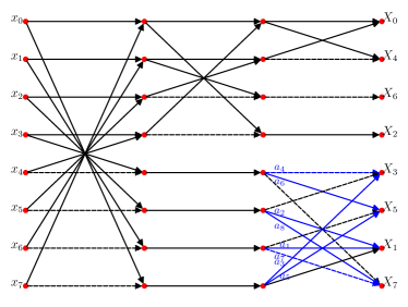
Figure 1: SFG for the proposed multiparametric transform. Solid and dashed arrows represent multiplication by 1 and -1, respectively. Blue arrows relate to the chosen parameter vector $\mathbf{a}$.

The presented fast algorithm computes $\mathbf{T(a)}$ at additive and bit-shift complexities given by

$$\mathcal{A}(\mathbf{a})=22-\sum^{8}_{i=1}\mathcal{I}_{\{0\}}(a_{i})\;\text{and}\;\mathcal{S}(\mathbf{a})=\sum^{8}_{i=1}\mathcal{I}_{\left\{\frac{1}{2},2\right\}}(a_{i}),$$ (5)

where $\mathcal{I}_{\Theta}(\theta)$ is the indicator function that returns $1$ if $\theta\in\Theta$ and zero otherwise.

3 Optimization on the Multiparametric Class

To select which of the transforms are representative for the signal decorrelation problem, we set up a computational procedure that searches for optimal transformations according to preset objective metrics [60, 17]. Besides the orthogonality property, three types of figures of merit are considered for rating a given approximate DCT: (i) the arithmetic complexity for measuring its computational cost, (ii) proximity measures to the DCT in a euclidean distance sense, and (iii) coding metrics for assessing its decorrelation capabilities. By construction, the proposed parametrization has zero multiplicative cost. Thus, for assessing the arithmetic complexity, we considered the total additive and bit-shift complexity given in (5). For measuring the transform similarity to the DCT, we adopted the total error energy [19] and the mean square error (MSE) [16]. The coding capabilities of a given approximate DCT are often measured by the unified transform coding gain [36] and transform efficiency [16] metrics.

3.1 Orthogonality Constraint

Approximate transforms are often desired to be orthogonal [16] because orthogonality implies that both direct and inverse transforms share the same computing structures [2]. In fact, the inverse transform is obtained by transposition, which results in simpler software and hardware implementations [35].

In order to the matrix $\mathbf{T(a)}$ to posses an orthogonal vector basis, the nondiagonal elements of $\mathbf{T(a)}\cdot\mathbf{T(a)}^{\top}$ must be null. Thus, we have that

$$\mathbf{T(a)}\cdot\mathbf{T(a)}^{\top}=\begin{bmatrix}8&0&0&0&0&0&0&0\\ 0&\tau_{1}&0&\tau_{2}&0&\tau_{3}&0&\tau_{4}\\ 0&0&4&0&0&0&0&0\\ 0&\tau_{2}&0&\tau_{5}&0&\tau_{6}&0&\tau_{7}\\ 0&0&0&0&8&0&0&0\\ 0&\tau_{3}&0&\tau_{6}&0&\tau_{8}&0&\tau_{9}\\ 0&0&0&0&0&0&4&0\\ 0&\tau_{4}&0&\tau_{7}&0&\tau_{9}&0&\tau_{10}\\ \end{bmatrix},$$ (6)

where $\tau_{1}=2a_{1}^{2}+2a_{2}^{2}+2$, $\tau_{2}=-2a_{2}+2a_{3}$, $\tau_{3}=-2a_{1}+2a_{5}$, $\tau_{4}=-2a_{1}a_{7}+2a_{2}a_{8}$, $\tau_{5}=2a_{3}^{2}+2a_{4}^{2}+2$, $\tau_{6}=2a_{3}a_{5}-2a_{4}a_{6}$, $\tau_{7}=2a_{4}-2a_{8}$, $\tau_{8}=2a_{5}^{2}+2a_{6}^{2}+2$, $\tau_{9}=-2a_{6}+2a_{7}$, and $\tau_{10}=2a_{7}^{2}+2a_{8}^{2}+2$. Thus, the orthogonality conditions are

$$\tau_{2}=\tau_{3}=\tau_{4}=\tau_{6}=\tau_{7}=\tau_{9}=0,$$ (7)

$$\tau_{1}\neq 0,\tau_{5}\neq 0,\tau_{8}\neq 0,\tau_{10}\neq 0.$$ (8)

We obtain orthonormal transforms $\mathbf{\tilde{C}(a)}$—referred hereafter as DCT approximations—by means of normalizing the energy of the basis vectors [30], according to:

$$\mathbf{\tilde{C}(a)} =\mathbf{S(a)}\cdot\mathbf{T(a)},$$ (9)

where $\mathbf{S(a)}$ is a diagonal matrix computed by

$$\mathbf{S(a)} =\sqrt{\left(\mathbf{T(a)}\cdot\mathbf{T(a)}^{\top}\right)^{-1}},$$ (10)

and the square root operation is applied to each element of the argument matrix. Relying on the orthogonality property, we have that

$$\mathbf{S(a)} =\operatorname{diag}\left(\frac{1}{2\sqrt{2}},\frac{1}{\sqrt{\tau_{1}}},\frac{1}{2},\frac{1}{\sqrt{\tau_{5}}},\frac{1}{2\sqrt{2}},\frac{1}{\sqrt{\tau_{8}}},\frac{1}{2},\frac{1}{\sqrt{\tau_{10}}}\right).$$ (11)

If (7) and (8) are satisfied, then $\tilde{\mathbf{C}}(\mathbf{a})\cdot\tilde{\mathbf{C}}(\mathbf{a})^{\top}=\mathbf{I}_{8}$.

3.2 Arithmetic Complexity of the Approximation

The arithmetic complexity associated to the approximate DCT $\mathbf{\tilde{C}(a)}$ can be regarded as identical to the complexity of the low-complexity matrix $\mathbf{T(a)}$, because the scaling factors of the diagonal matrix $\mathbf{S(a)}$ can be merged into the quantization step of image and video enconders [48, 19, 12, 11, 52]. Thus, the arithmetic complexity assessment presented in (5) is applicable to both direct and inverse transforms, because the same fast algorithm is applicable to both cases.

3.3 Multicriteria Optimization

By considering: (i) the search space implied by the proposed parametrization, (ii) the orthogonality condition, and (iii) the above discussed figures of merit, we have the following multicriteria minimization problem:

$$\begin{split}\mathbf{a}_{\text{opt}}=\arg\min_{\mathbf{a}}\Big{\{}\epsilon(\tilde{\mathbf{C}}(\mathbf{a})),\operatorname{MSE}(\tilde{\mathbf{C}}(\mathbf{a})),-C_{g}^{*}(\tilde{\mathbf{C}}(\mathbf{a})),-\eta(\tilde{\mathbf{C}}(\mathbf{a})),\mathcal{A}(\mathbf{a}),\mathcal{S}(\mathbf{a})\Big{\}}\end{split}$$ (12)

subject to

$$\begin{cases}a_{i}\in\mathcal{C},\quad i=1,2,\ldots,8\\ \tau_{j}=0,\quad j=2,3,4,6,7,9\\ \tau_{k}\neq 0,\quad k=1,5,8,10\end{cases},$$

where $\epsilon(\cdot)$, $\operatorname{MSE}(\cdot)$, $C_{g}^{*}(\cdot)$, and $\eta(\cdot)$ compute the total error energy, MSE, unified transform coding gain, and transform efficiency of the argument transform. Note that coding metrics are sought to be maximized, whereas proximity to the DCT (error) and complexity should be minimized. The obtained optimal parameter vectors $\mathbf{a}_{\text{opt}}$ readily define the optimal transforms according to $\tilde{\mathbf{C}}(\mathbf{a}_{\text{opt}})$.

3.4 Optimal 8-point Transforms

The solution of (12) results on seven optimal 8-point transforms, which are listed in Table 1. For simplicity, hereafter, we denote the optimal transforms as $\mathbf{\tilde{C}}_{8}^{(j)}$, where $j=1,2,\ldots,7$. Three of the optimal transformations are state-of-the-art approximate DCTs already archived in literature, namely: the MRDCT [5], the transform by Oliveira et al. (OCBT) [49], and the RDCT [19] ($j=1,2,6$, respectively). The transform OCBT can also be found in [15] and [17]. However, to the best of our knowledge, the remaining four transforms presented in Table 1 are novel contributions to the literature ($j=3,4,5,7$).

Table 1: Optimal 8-point DCT approximations in the proposed class.

$j$	$\mathbf{a}_{\text{opt}}$	Description
1	[0 0 0 0 0 0 0 0]⊤	MRDCT [5]
2	[1 0 0 0 1 0 0 0]⊤	OCBT [49]
3	[1 0 0 1 1 0 0 1]⊤	New
4	[1 0 0 0.5 1 0 0 0.5]⊤	New
5	[1 1 1 -1 1 -1 -1 -1]⊤	New
6	[1 1 1 1 1 1 1 1]⊤	RDCT [19]
7	[1 0.5 0.5 1 1 0.5 0.5 1]⊤	New

Table 2 presents proximity and coding measurements relative to the DCT along with the arithmetic complexity associated to each of the obtained optimal 8-point transforms. Hereafter, in all the tables, the best results are highlighted in boldface. The approximation $\mathbf{\tilde{C}}_{8}^{(1)}$ (MRDCT) still holds the lowest additive cost for an approximate DCT requiring 14 additions only. Also the approximation $\mathbf{\tilde{C}}_{8}^{(6)}$ (RDCT) still maintain its status as the transformation with the the smallest total error energy measure. On the other hand, among the optimal transforms, the proposed transform $\mathbf{\tilde{C}}_{8}^{(7)}$ possesses the lowest MSE measurement, a very low error energy, and attains the highest coding gain and efficiency.

Table 2: Measurements for the optimal 8-point approximate DCTs.

$j$	$\epsilon(\cdot)$	MSE$(\cdot)$	$C_{g}^{*}(\cdot)$	$\eta(\cdot)$	$\mathcal{A}(\cdot)$	$\mathcal{S}(\cdot)$
1	8.6592	0.0594	7.3326	80.8969	14	0
2	6.8543	0.0275	7.9118	85.6419	16	0
3	5.0493	0.0246	7.9207	85.3793	18	0
4	5.0184	0.0241	8.1102	86.8665	18	2
5	16.0260	0.0333	8.1571	88.1932	22	0
6	1.7945	0.0098	8.1827	87.4297	22	0
7	2.1443	0.0083	8.4261	89.1383	22	4

For comparison purposes, we compile in Table 3 the performance measurements of representative competing transforms found in the literature: the series of transforms introduced by Bouguezel, Ahmad and Swamy (BAS₁ [10], BAS₂ [11], BAS₃ [14], BAS₄ [12] and BAS₅ [13]); the level 1 transform (LO) by Lengwehasatit and Ortega [40]; and the approximations reported in [60], [48], and  [17] referred to as TBC, OCBSML, and CSBC, respectively. Such selected transforms were chosen so that they are not members of the proposed class of approximations. Hereafter, in the tables, the superscript on CSBC and TBC identifies the instance from the class of transforms reported in the original papers [17, 60]; whereas the one next to BAS₅ indicates the quantity considered in the parametric formulation from [13]. The DCT and the integer DCT from HEVC [43] demand much more resources and are not used in the following comparisons.

Table 3: Measurements for the competing 8-point approximate DCTs.

Transform	$\epsilon(\cdot)$	MSE$(\cdot)$	$C_{g}^{*}(\cdot)$	$\eta(\cdot)$	$\mathcal{A}(\cdot)$	$\mathcal{S}(\cdot)$
CSBC(1) [17]	6.8543	0.0275	7.9118	85.6419	16	0
BAS${}_{5}^{(0)}$ [13]	26.8642	0.0710	7.9118	85.6419	16	0
BAS2 [11]	6.8543	0.0275	7.9126	85.3799	18	0
TBC(6) [60]	8.6592	0.0588	7.3689	81.1788	18	0
BAS${}_{5}^{(1)}$ [13]	26.8642	0.0710	7.9126	85.3799	18	0
BAS1 [10]	5.9294	0.0238	8.1194	86.8626	18	2
BAS${}_{5}^{(1/2)}$ [13]	26.4018	0.0678	8.1194	86.8626	18	2
CSBC(9) [17]	4.1203	0.0214	8.1199	86.7297	20	3
TBC(5) [60]	7.4138	0.0530	7.5753	83.0846	20	10
BAS3 [14]	35.0639	0.1023	7.9461	85.3138	24	0
LO [40]	0.8695	0.0061	8.3902	88.7023	24	2
BAS4 [12]	4.0935	0.0210	8.3251	88.2182	24	4
OCBSML [48]	1.2194	0.0046	8.6337	90.4615	24	6

To derive fair comparison, hereafter, we confront transforms possessing approximately the same arithmetic complexity. The new approximate DCT $\mathbf{\tilde{C}}_{8}^{(3)}$ outperforms the other low-complexity transforms requiring 18 additions in terms of error energy, MSE, and coding gain. The proposed transform $\mathbf{\tilde{C}}_{8}^{(4)}$ achieves smaller total error energy and the higher efficiency if compared with other approaches that require exactly 18 addition and 2 bit-shifting operations. The introduced transform $\mathbf{\tilde{C}}_{8}^{(5)}$ is more efficient than $\mathbf{\tilde{C}}_{8}^{(6)}$, but has smaller error energy, MSE and coding gain. No other listed transform demands exactly 22 additions. The DCT approximation $\mathbf{\tilde{C}}_{8}^{(7)}$ has no direct competitor found. Note, however, that $\mathbf{\tilde{C}}_{8}^{(7)}$ ranks in the third and fourth places in terms of MSE and total error energy, and attains the second place according to coding gain and efficiency measurements if compared with any other transform listed in Tables 2 and 3. Together with outstanding DCT-like transforms as $\mathbf{\tilde{C}}_{8}^{(6)}$ (RDCT) [19], LO [40] and OCBSML [48], the proposed transform $\mathbf{\tilde{C}}_{8}^{(7)}$ composes the new state-of-the-art on 8-point approximate DCTs.

4 Scaling 8-point to 16- and 32-point Transforms

Widely popular image and video coding standards—e.g. JPEG [64], H.262 [44], and H.264 [56]—employ the 8-point DCT for decorrelation, thus attracting the community efforts to that specific length [5, 28, 13]. More recently, the HEVC standard proposed to use DCT-like transforms of different lengths: $4$, $8$, $16$, and $32$ [46]. Such design choice enhances the compression of high-resolution video and improves the coding efficiency mainly at low bit-rates [66]. Generally, small-sized transforms cope with textured regions, whereas the large-sized ones act on smoother video content [54].

Therefore, there is a demand for low-cost DCT-like transforms, since the computational complexity of the exact DCT grows non-linearly [35]. Nevertheless, there are only a few works focusing on natively approximating the 16- or 32-point DCT [22, 23, 6]. A practical approach for scaling up 8-point transforms to larger transforms of size 16 and 32 consists of applying the method proposed by Jridi, Alfalou, and Meher (JAM) [35]. In a nutshell, the JAM method takes two instances of a low-complexity multiplierless transform of length $N$ to compose another transform of length $2N$. The total arithmetic complexity of the $2N$-point transform is kept low. It requires twice the number of bit-shifts and twice plus $2N$ additions demanded by the original $N$-point transform. Originally, the RDCT ($\mathbf{\tilde{C}}_{8}^{(6)}$) was used in the scaling process introduced in [35]. For brevity, we refer the reader to the original paper for more details about the scalable JAM method [35].

4.1 16-point Scaled Transforms

The proposed optimal 8-point transforms were submitted to the JAM method in order to generate scaled transforms of length 16. Table 4 summarizes the quality and complexity measurements for these DCT approximations. To the best of our knowledge, five from the seven derived 16-point transforms are novel contributions to the literature. The 16-point transforms $\mathbf{\tilde{C}}_{16}^{(6)}$ and $\mathbf{\tilde{C}}_{16}^{(2)}$ were introduced in (JAM) [35] and (CSBC⁽¹⁾) [17], respectively. The results from Table 2 and Table 4 shows that the JAM scaling could roughly transfer the performance from the 8-point to the 16-point approximations.

Table 4: Measurements for the scaled 16-point approximate DCTs.

$j$	$\epsilon(\cdot)$	MSE$(\cdot)$	$C_{g}^{*}(\cdot)$	$\eta(\cdot)$	$\mathcal{A}(\cdot)$	$\mathcal{S}(\cdot)$
1	29.7486	0.0935	7.5816	66.0681	44	0
2	25.1300	0.0674	8.1577	70.9808	48	0
3	21.5172	0.0646	8.1664	70.5897	52	0
4	21.6809	0.0644	8.3560	72.1975	52	4
5	41.1430	0.0707	8.4036	73.8217	60	0
6	14.7402	0.0506	8.4285	72.2296	60	0
7	15.8124	0.0507	8.6711	75.8460	60	8

Table 5 lists representative 16-point DCT approximations: the BAS₃ and BAS₄ transforms, the approximations in [22] (SOBCM) and [23] (SBCKMK); and the approximation in [6] (BCEM). We also included JAM-scaled versions of the 8-point approximations CSBC [17] and OCBSML [48].

Table 5: Measurements for competing 16-point approximate DCTs.

Transform	$\epsilon(\cdot)$	MSE$(\cdot)$	$C_{g}^{*}(\cdot)$	$\eta(\cdot)$	$\mathcal{A}(\cdot)$	$\mathcal{S}(\cdot)$
SOBCM [22]	40.9996	0.0947	7.8573	67.6078	44	0
CSBC(4) [17]	20.8777	0.0648	8.1587	71.4837	52	2
CSBC(5) [17]	23.0211	0.0641	8.3653	71.8269	52	4
CSBC(9) [17]	18.7688	0.0615	8.3663	72.3414	56	6
CSBC(10) [17]	19.6427	0.0621	8.3659	72.1040	56	6
SBCKMK [23]	30.3230	0.0639	8.2950	70.8315	60	0
CSBC(13) [17]	18.5159	0.0599	8.3647	72.6288	60	4
BAS3 [14]	97.8678	0.4520	8.1941	70.6465	64	0
BAS4 [12]	16.4071	0.0564	8.5208	73.6345	64	8
OCBSML [48]	13.7035	0.0474	8.8787	76.8108	64	12
BCEM [6]	8.0806	0.0465	7.8401	65.2789	72	0

The proposed approximation $\mathbf{\tilde{C}}_{16}^{(1)}$ outperforms SOBCM in proximity metrics, requiring 44 additions only. Transform $\mathbf{\tilde{C}}_{16}^{(3)}$ has no direct competitor with the same arithmetic cost but performs close to CSBC⁽⁴⁾ and CSBC⁽⁵⁾, which require two and four extra bit-shifting operations, respectively. The DCT approximation $\mathbf{\tilde{C}}_{16}^{(4)}$ attains smaller error energy and higher efficiency when compared with CSBC⁽⁵⁾. The proposed approximate DCT $\mathbf{\tilde{C}}_{16}^{(5)}$ outperforms SBCKMK in coding metrics, and achieves better transform efficiency than $\mathbf{\tilde{C}}_{16}^{(6)}$. The transform $\mathbf{\tilde{C}}_{16}^{(7)}$ ranks on the fourth place in terms of proximity to the DCT, and is the second best-performing in coding metrics among the transforms in Tables 4 and 5.

4.2 32-point Scaled Transforms

By invoking the JAM method twice, we can scale 8-point transforms and obtain 32-point DCT approximations. The obtained error and coding measurements as well as the arithmetic complexity of the obtained 32-point transforms are presented in Table 6. We found $\mathbf{\tilde{C}}_{32}^{(1)}$, $\mathbf{\tilde{C}}_{32}^{(3)}$, $\mathbf{\tilde{C}}_{32}^{(4)}$, $\mathbf{\tilde{C}}_{32}^{(5)}$, and $\mathbf{\tilde{C}}_{32}^{(7)}$ as contributions to the literature. The scaled transforms $\mathbf{\tilde{C}}_{32}^{(2)}$ and $\mathbf{\tilde{C}}_{32}^{(6)}$ coincide with 32-point versions of CSBC⁽¹⁾ and JAM proposal, respectively. Peering approaches and their respective quality and cost measurements are listed in Table 7. Excepting for SOBCM, SBCKMK, and BCEM which are 16-point transforms only, the other competing approaches are the 32-point versions of those in Table 5. Namely, we consider the 32-point BAS₃, BAS₄, CSBC and OCBSML transforms.

Table 6: Measurements for the scaled 32-point approximate DCTs.

$j$	$\epsilon(\cdot)$	MSE$(\cdot)$	$C_{g}^{*}(\cdot)$	$\eta(\cdot)$	$\mathcal{A}(\cdot)$	$\mathcal{S}(\cdot)$
1	77.7215	0.1497	7.6584	52.2784	120	0
2	68.1287	0.1278	8.2306	56.1785	128	0
3	61.2029	0.1251	8.2393	55.8320	136	0
4	61.7212	0.1252	8.4287	57.1200	136	8
5	96.7291	0.1302	8.4771	58.4748	152	0
6	48.0956	0.1124	8.5010	56.9700	152	0
7	50.4638	0.1133	8.7429	60.4018	152	16

Table 7: Measurements for competing 32-point approximate DCTs.

Transform	$\epsilon(\cdot)$	MSE$(\cdot)$	$C_{g}^{*}(\cdot)$	$\eta(\cdot)$	$\mathcal{A}(\cdot)$	$\mathcal{S}(\cdot)$
CSBC(4) [17]	59.4743	0.1253	8.2320	56.7808	136	4
CSBC(5) [17]	63.9307	0.1249	8.4382	56.7210	136	8
CSBC(6) [17]	60.6931	0.1218	8.2516	56.4665	144	0
CSBC(9) [17]	55.2764	0.1224	8.4396	57.3346	144	12
CSBC(10) [17]	56.3736	0.1227	8.4390	56.9787	144	12
CSBC(13) [17]	52.9321	0.1186	8.4389	57.5669	152	8
BAS3 [14]	192.1804	0.7609	8.2693	55.9114	160	0
BAS4 [12]	117.0653	0.2411	8.4998	58.4956	160	16
OCBSML [48]	46.2658	0.1104	8.9505	61.0272	160	24

To the best of our knowledge, the novel transform $\mathbf{\tilde{C}}_{32}^{(1)}$ possesses the smaller arithmetic complexity archived in the literature. Transform $\mathbf{\tilde{C}}_{32}^{(3)}$ has smaller error energy than CSBC⁽⁵⁾, smaller MSE than CSBC⁽⁴⁾, and higher coding gain than CSBC⁽⁴⁾, while requiring fewer arithmetic operations. The transform $\mathbf{\tilde{C}}_{32}^{(4)}$ outperforms CSBC⁽⁵⁾ in terms of error energy and efficiency, both requiring 136 additions and 8 bit-shifts. $\mathbf{\tilde{C}}_{32}^{(5)}$ has no direct competitors, but presents competitive coding gain and transform efficiency measurements. Once again, $\mathbf{\tilde{C}}_{32}^{(5)}$ stands out, by ranking on third and second places for proximity to the exact DCT and coding capabilities, respectively, among all considered 32-point transforms.

5 Application to Image and Video Coding

In this section, we describe computational experiments on both still-image and video compression aiming at assessing the behavior of the selected transforms on such applications.

5.1 Still-Image Compression

We performed a JPEG-like experiment to assess the optimal 8-point DCT-like transforms and their scaled 16- and 32-point counterparts in the context of still-image compression. The experiment consisted of subdividing the input image into disjoint blocks $\mathbf{A}$ of size $N\times N$. Each block was individually processed as follows. The direct transformation was applied to $\mathbf{A}$ according to $\mathbf{B}=\mathbf{T}_{N}\cdot\mathbf{A}\cdot\mathbf{T}_{N}^{\top}$, where $\mathbf{T}_{N}$ is a $N$-point orthogonal transform and $\mathbf{B}$ is the resulting transformed block. Using the zig-zag scan sequence [64], we kept the first $r$ coefficients while setting the remaining coefficients to zero. The truncated block is represented by $\mathbf{\tilde{B}}$. Then, we applied the inverse transformation to each block $\mathbf{\tilde{B}}$ through $\mathbf{\tilde{A}}=\mathbf{T}^{\top}_{N}\cdot\mathbf{\tilde{B}}\cdot\mathbf{T}_{N}$. The correct rearrangement of all the blocks $\mathbf{\tilde{A}}$ resulted on a $\mathbf{T}_{N}$-compressed version of the input image at compression rate $r/N^{2}$.

In this experiment, we evaluated the performance of a given transform $\mathbf{T}_{N}$ by objectively assessing the quality of the compressed image. For that end, we employed the peak signal-to-noise-ratio (PSNR) [32] and the structural similarity index (SSIM) [65] following the procedure described in [15, 35, 28, 13, 10, 11]. We also include results for the learned perceptual image patch similarity (LPIPS) [68], a perceptual-based metric, which correlates to the mean opinion score [37]. We report the averaged results for 45 $512\times 512$ grayscale images from a public database [62], with $r$ varying from $1$ to approximately $0.75N^{2}$, with $N=8,16,32$. The chosen quantities of retained coefficients $r$ roughly correspond to compression rates ranging from $25\%$ to $99\%$.

5.1.1 Results for the 8-point Approximations

Fig. 2(a) and Fig. 2(b) depict the average SSIM and PSNR measurements, respectively, for selected 8-point transforms. Namely, we separated the best-performing novel transform $\mathbf{\tilde{C}}^{(7)}_{8}$, and the followings competing methods: LO, OCBSML, RDCT, BAS₄, and the exact DCT. Note that the transform $\mathbf{\tilde{C}}^{(7)}_{8}$ achieves the second-best PSNR gains for high compression rates ($r<5$). It also performs comparably to the LO approximation for intermediary compression rates ($20<r<35$), and outperforms the RDCT in all the cases. Similar results are obtained for the SSIM measurements. Fig. 2(c) depicts the LPIPS measurements, suggesting that approximate transforms can outperform the DCT for some $r$ values.

Complementary, we provide the SSIM, PSNR and LPIPS gains per addition operation—which can be useful for comparing transforms of different complexities. Bit-shifting operations are often regarded as virtually costless in hardware implementations [47, 48], and are thus suppressed in our analysis. Fig. 2(d) and Fig. 2(e) show that the proposed DCT-like transform $\mathbf{\tilde{C}}^{(7)}_{8}$ has consistently higher SSIM gains per addition unit, also reflected in terms of PSNR measurements. The RDCT, well-known for its outstanding coding capabilities, behaves similarly to $\mathbf{\tilde{C}}^{(7)}_{8}$, but presenting slightly worse results. Fig. 2(f) shows the LPIPS values per addition, where $\mathbf{\tilde{C}}^{(7)}_{8}$ roughly compares to LO, BAS₄, and OCBSML.

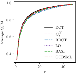
(a) Average SSIM

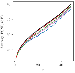
(b) Average PSNR

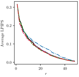
(c) Average LPIPS

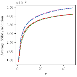
(d) Average SSIM / $\mathcal{A}(\cdot)$

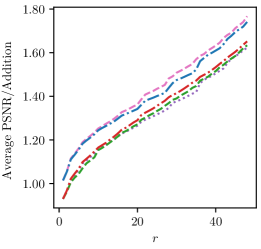
(e) Average PSNR / $\mathcal{A}(\cdot)$

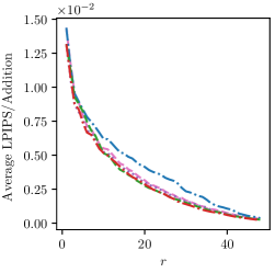
(f) Average LPIPS / $\mathcal{A}(\cdot)$

Figure 2: Image compression results for novel and competing 8-point DCT approximations. The legends are shared across the multiple graphics.

5.1.2 Results for the 16-point Approximations

Fig. 3(a) and Fig. 3(b) present the average SSIM and PSNR measurements for the experiment involving 16-point transforms. We separated the scaled transforms $\mathbf{\tilde{C}}^{(1)}_{16}$, $\mathbf{\tilde{C}}^{(7)}_{16}$, and $\mathbf{\tilde{C}}^{(6)}_{16}$, besides peering approaches like BAS₄, SBCKMK, SOBCM, OCBSML, and the exact DCT. The proposed transform $\mathbf{\tilde{C}}^{(7)}_{16}$ outperforms all other approximate DCTs, excepting for OCBSML, for $r<140$. The transform $\mathbf{\tilde{C}}^{(1)}_{16}$ achieves comparable PSNR and SSIM measurements roughly for $50<r<100$ if compared with SOBCM, both requiring 44 additions only. Fig. 3(c) show the LPIPS scores. The results indicate $\mathbf{\tilde{C}}^{(7)}_{16}$ and OCBSML as best-performing together with the exact DCT.

The SSIM, PSNR, and LPIPS curves normalized by the number of additions required by the selected low-complexity 16-point transforms are shown in Fig. 3(d), Fig. 3(e), and Fig. 3(f), respectively. The curves indicate a favorable performance for $\mathbf{\tilde{C}}^{(1)}_{16}$ in terms of SSIM/PSNR gain per addition unit. The approximate DCT $\mathbf{\tilde{C}}^{(7)}_{16}$ has comparable SSIM gain per addition regarding $\mathbf{\tilde{C}}^{(6)}_{16}$, and consistently outperforms SBCKMK, BAS₄ and OCBSML both in normalized PSNR and SSIM gains per addition operation.

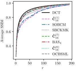
(a) Average SSIM

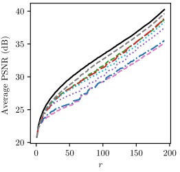
(b) Average PSNR

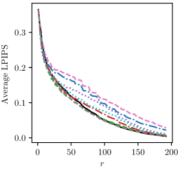
(c) Average LPIPS

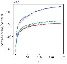
(d) Average SSIM / $\mathcal{A}(\cdot)$

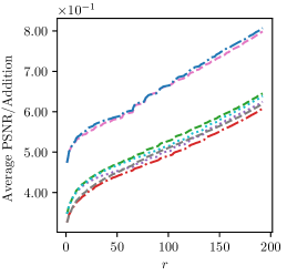
(e) Average PSNR / $\mathcal{A}(\cdot)$

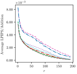
(f) Average LPIPS / $\mathcal{A}(\cdot)$

Figure 3: Image compression results for proposed and competing 16-point DCT approximations. The legends are shared across the multiple graphics.

5.1.3 Results for the 32-point Approximations

Finally, the mean SSIM and PSNR curves for selected 32-point transforms are shown in Fig. 4(a) and Fig. 4(b). We exhibit the scaled DCT approximations $\mathbf{\tilde{C}}^{(1)}_{32}$, $\mathbf{\tilde{C}}^{(2)}_{32}$, $\mathbf{\tilde{C}}^{(6)}_{32}$, and $\mathbf{\tilde{C}}^{(7)}_{32}$, besides peering methods like BAS₄, OCBSML, and the exact DCT. The transform $\mathbf{\tilde{C}}^{(7)}_{32}$ performs better than all other competing approaches, except for OCBSML. Although $\mathbf{\tilde{C}}^{(1)}_{32}$ performs relatively poorly, it saves up to 25% of the total number of additions when compared with the other approaches and does not require any bit-shifting operation. Fig. 4(c) shows that the DCT is outperformed by $\mathbf{\tilde{C}}^{(6)}_{32}$ and OCBSML for $r<500$ values in terms of LPIPS.

Fig. 4(d), Fig. 4(e), and  4(f) depict the SSIM, PSNR, and LPIPS gains per addition operation for the considered 32-point transforms, respectively. The method $\mathbf{\tilde{C}}^{(1)}_{32}$ achieves the best SSIM and PSNR gains per addition unit when compared with the other approaches for practically any $r$ value. The curves also show that the proposed transform $\mathbf{\tilde{C}}^{(7)}_{32}$ presents consistently better results than the remaining approaches, $\mathbf{\tilde{C}}^{(6)}_{32}$, BAS₄, and OCBSML. LPIPS by addition unit further highlights the results of $\mathbf{\tilde{C}}^{(6)}_{32}$ and OCBSML.

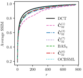
(a) Average SSIM

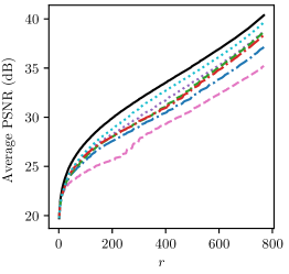
(b) Average PSNR

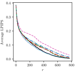
(c) Average LPIPS

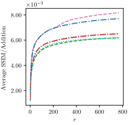
(d) Average SSIM / $\mathcal{A}(\cdot)$

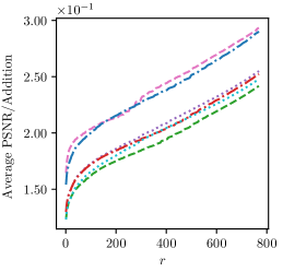
(e) Average PSNR / $\mathcal{A}(\cdot)$

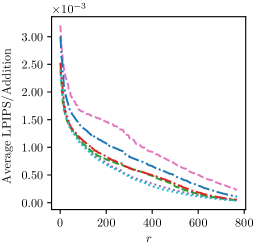
(f) Average LPIPS / $\mathcal{A}(\cdot)$

Figure 4: Image compression results for the proposed and competing 32-point DCT approximations. The legends are shared across the multiple graphics.

Fig. 5 exemplifies the compression of the “Lena” image by selected transforms: $\mathbf{\tilde{C}}^{(1)}_{N}$ and $\mathbf{\tilde{C}}^{(7)}_{N}$, and the DCT for $N\in\{8,16,32\}$. We select $r$ values so that the compression rate is roughly 84%. Note that transforms $\mathbf{\tilde{C}}^{(7)}_{8}$, $\mathbf{\tilde{C}}^{(7)}_{16}$, and $\mathbf{\tilde{C}}^{(7)}_{32}$ have high PSNR values and virtually no visual degradation.

(a) PNSR = 31.6393 dB

(b) PNSR = 26.6691 dB

(c) PNSR = 30.4560 dB

(d) PNSR = 32.0423 dB

(e) PNSR = 26.6102 dB

(f) PNSR = 30.3091 dB

(g) PNSR = 32.5315 dB

(h) PNSR = 26.6179 dB

(i) PNSR = 30.3445 dB

Figure 5: “Lena” image compressed by (a)(d)(g) the DCT, (b)(e)(h) $\mathbf{\tilde{C}}^{(1)}_{N}$, and (c)(f)(i) $\mathbf{\tilde{C}}^{(7)}_{N}$ for (a–c) $N=8$, (d–f) $N=16$, and (g–i) $N=32$. The parameter $r$ is set to 10, 40, and 155, for $N=8,16,32$, respectively.

5.2 Video Coding

This section reports the suitability results of the introduced best-performing 8-point transform—$\mathbf{\tilde{C}}_{8}^{(7)}$—together with its scaled 16- and 32-point versions to video coding. We also included in our analysis the optimal 8-point transform $\mathbf{\tilde{C}}_{8}^{(1)}$ (MRDCT) and its scaled versions of lengths 16 and 32 since they possess a very low arithmetic complexity and still compelling coding results. In this experiment, we embedded the two groups of 8-, 16- and 32-point transforms into a publicly available HEVC reference software [34], and then assessed the performance of the resulting systems. For simplicity, hereafter we refer to these groups as $\mathbf{\tilde{C}}^{(1)}_{\text{group}}$ and $\mathbf{\tilde{C}}^{(7)}_{\text{group}}$. The core HEVC integer DCT (intDCT) transforms of lengths 8, 16 and 32 require 50, 186, and 682 additions and 30, 86, and 287 bit-shifts, respectively [43]. The 4-point intDCT HEVC transform requires no approximation because it is already a low-complexity multiplierless transformation.

We encoded the first 100 frames of representative video sequences from each A to F class according to the recommendations detailed in the Common Test Conditions (CTC) document [9]. The following 8-bit videos were selected: “PeopleOnStreet” (2560$\times$1600 at 30 fps), “BasketballDrive” (1920$\times$1080 at 50 fps), “RaceHorses” (832$\times$480 at 30 fps), “BlowingBubbles” (416$\times$240 at 50 fps), “KristenAndSara” (1280$\times$720 at 60 fps), and “BasketballDrillText” (832$\times$480 at 50 fps). We set the encoding parameters for the Main profile and All-Intra (AI), Random Access (RA), Low Delay B (LD-B), and Low Delay P (LD-P) configurations according to the CTC document. Our experiments consider varying the quantization parameter (QP) in $\{22,27,32,37\}$ as recommended by the CTC documentation [9].

The reference software itself measures the MSE and PSNR for each frame and color channel (in YUV color space), and we compute the YUV-PSNR [46]. We used these measurements for each QP value for computing the Bjøntegaard’s delta PSNR (BD-PSNR) and delta rate (BD-Rate) [7, 26] for the two groups of transforms and the four coding configurations. Table 8 lists the obtained BD-PSNR and BD-Rate measurements. Fig. 6 presents the corresponding rate-distortion (RD) curves, which are interpolated by cubic splines for better visualization [20, 26]. Although the proposed transforms present some quality loss, they require a fraction of the required operations by HEVC core transforms.

The transform $\mathbf{\tilde{C}}^{(7)}_{\text{group}}$ obtained much better results than $\mathbf{\tilde{C}}^{(1)}_{\text{group}}$ for all configuration modes and video sequences. These findings corroborate the results from the still-image compression experiments from Section 5.1. Note that replacing the original HEVC transforms by $\mathbf{\tilde{C}}^{(7)}_{\text{group}}$ results in a loss of no more than 0.54 dB in AI configuration, which may be negligible depending on the target application.

Table 8: Average BD-PSNR and BD-Rate for the transforms $\mathbf{\tilde{C}}^{(1)}_{\text{group}}$ and $\mathbf{\tilde{C}}^{(7)}_{\text{group}}$ embedded into the HEVC reference software

Config.	Video sequence	BD-PSNR (dB)		BD-Rate (%)
		$\mathbf{\tilde{C}}^{(1)}_{\text{group}}$	$\mathbf{\tilde{C}}^{(7)}_{\text{group}}$	$\mathbf{\tilde{C}}^{(1)}_{\text{group}}$	$\mathbf{\tilde{C}}^{(7)}_{\text{group}}$
AI	“PeopleOnStreet”	$-0.5405$	$\mathbf{-0.4156}$	$10.7981$	$\mathbf{8.2472}$
	“BasketballDrive”	$-0.3312$	$\mathbf{-0.2013}$	$13.0744$	$\mathbf{7.7961}$
	“RaceHorses”	$-0.6681$	$\mathbf{-0.5373}$	$8.7455$	$\mathbf{7.0180}$
	“BlowingBubbles”	$-0.2569$	$\mathbf{-0.1568}$	$4.5457$	$\mathbf{2.7863}$
	“KristenAndSara”	$-0.4717$	$\mathbf{-0.3225}$	$9.8382$	$\mathbf{6.6716}$
	“BasketballDrillText”	$-0.2049$	$\mathbf{-0.1320}$	$4.0161$	$\mathbf{2.5766}$
RA	“PeopleOnStreet”	$-0.2908$	$\mathbf{-0.2132}$	$7.1735$	$\mathbf{5.2135}$
	“BasketballDrive”	$-0.2560$	$\mathbf{-0.1609}$	$12.1530$	$\mathbf{7.5263}$
	“RaceHorses”	$-0.9507$	$\mathbf{-0.6369}$	$16.0780$	$\mathbf{10.9197}$
	“BlowingBubbles”	$-0.2009$	$\mathbf{-0.1119}$	$5.4653$	$\mathbf{3.0192}$
	“BasketballDrillText”	$-0.2490$	$\mathbf{-0.1704}$	$6.2465$	$\mathbf{4.2235}$
LD-B	“BasketballDrive”	$-0.2381$	$\mathbf{-0.1537}$	$10.6718$	$\mathbf{6.7131}$
	“RaceHorses”	$-0.9274$	$\mathbf{-0.6399}$	$14.5320$	$\mathbf{10.1138}$
	“BlowingBubbles”	$-0.2023$	$\mathbf{-0.1122}$	$5.6422$	$\mathbf{3.0933}$
	“KristenAndSara”	$-0.2351$	$\mathbf{-0.1640}$	$8.2957$	$\mathbf{5.7539}$
	“BasketballDrillText”	$-0.2895$	$\mathbf{-0.2054}$	$7.6528$	$\mathbf{5.3746}$
LD-P	“BasketballDrive”	$-0.2411$	$\mathbf{-0.1539}$	$10.6911$	$\mathbf{6.7416}$
	“RaceHorses”	$-0.8873$	$\mathbf{-0.6207}$	$13.7702$	$\mathbf{9.7240}$
	“BlowingBubbles”	$-0.1890$	$\mathbf{-0.1087}$	$5.3818$	$\mathbf{3.0557}$
	“KristenAndSara”	$-0.2227$	$\mathbf{-0.1493}$	$8.1583$	$\mathbf{5.5457}$
	“BasketballDrillText”	$-0.2697$	$\mathbf{-0.1960}$	$7.2204$	$\mathbf{5.2078}$

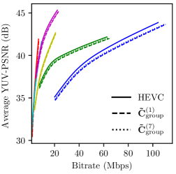
(a) AI

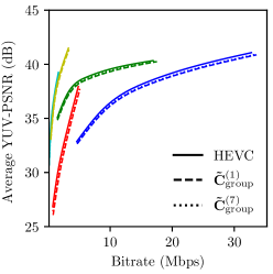
(b) RA

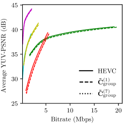
(c) LD-B

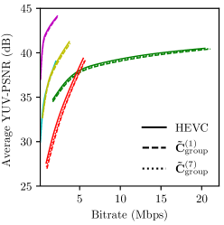
(d) LD-P

Figure 6: RD curves for different configuration modes and video sequences. Curves associated to “PeopleOnStreet”, “BasketballDrive”, “RaceHorses”, “BlowingBubbles”, “BasketballDrillText”, and “KristenAndSara” are represented by colors blue, green, red, cyan, yellow, and magenta, respectively.

Fig. 7 depicts the eighteenth frame of the “BasketballDrillText” video sequence encoded using the original HEVC transform suit compared with the results from the transform groups $\mathbf{\tilde{C}}^{(1)}_{\text{group}}$ and $\mathbf{\tilde{C}}^{(7)}_{\text{group}}$. We also provide the YUV-PSNR measurements for the selected frame. These results consider the four configuration modes and QPs. Note that there is no visually noticeable degradation associated to the approximate DCTs. These results suggest that the original HEVC transforms can be substituted by $\mathbf{\tilde{C}}^{(1)}_{\text{group}}$ or $\mathbf{\tilde{C}}^{(7)}_{\text{group}}$ without significant losses in image/video quality.

(a) YUV-PSNR = 42.5687 dB

(b) YUV-PSNR = 37.7729 dB

(c) YUV-PSNR = 35.1120 dB

(d) YUV-PSNR = 32.6642 dB

(e) YUV-PSNR = 42.4473 dB

(f) YUV-PSNR = 37.6475 dB

(g) YUV-PSNR = 34.9257 dB

(h) YUV-PSNR = 32.4855 dB

(i) YUV-PSNR = 42.4770 dB

(j) YUV-PSNR = 37.6561 dB

(k) YUV-PSNR = 35.0318 dB

(l) YUV-PSNR = 32.5330 dB

Figure 7: Compressed frame of “BasketballDrillText” using the (a–d) original HEVC, (e–h) $\mathbf{\tilde{C}}^{(1)}_{\text{group}}$ and (i–l) $\mathbf{\tilde{C}}^{(7)}_{\text{group}}$ transforms under different configuration modes and QP values. Results for (a)(e)(i) AI and $\mbox{QP}=22$, (b)(f)(j) RA and $\mbox{QP}=27$, (c)(g)(k) LD-B and $\mbox{QP}=32$, and (d)(h)(l) LD-P and $\mbox{QP}=37$.

6 Hardware Implementation

The proposed 8-point low-complexity transforms were implemented on a field programmable gate array (FPGA). The device adopted for the hardware implementation was the Xilinx Artix-7 XC7A35T-1CPG236C.

The designs use pipelined systolic architecture for implementing each of the transforms [4, 57]. The implemented blocks compute the transform using the fast algorithm outlined in (2) and displayed in Fig. 1. Each matrix in the factorization in (2) was implemented in a different sub-block, and were then wrapped together in a large module that implements the complete transform. Each sub-block that involves an arithmetic operation increases the wordlength in one bit in order to avoid overflow and its outputs are registered.

The designs were tested employing the scheme shown in Fig. 8, together with a state-machine serving as controller and connected to a universal asynchronous receiver-transmitter (UART) block. The UART core interfaces with the controller state machine using the ARM Advanced Microcontroller Bus Architecture Advanced eXtensible Interface 4 protocol. A personal computer (PC) communicates with the controller through the UART by sending a packet of eight 8-bit coefficients, corresponding to an input for the transform block. The values of the 8-bit coefficients are randomly generated integers in the interval $[-10,10]$. The set of the eight coefficients is then passed to the design and processed. Then the controller state machine sends the eight output coefficients back to the PC, which are then compared with the output of a software model used to ensuring the hardware design is correctly implemented.

Figure 8: Testbed architecture for testing the implemented designs.

Table 9 shows the hardware resource utilization for the new transforms in Table 1, together with the following 8-point transforms from the literature: RDCT [19], MRDCT [5], OCBSML [48], and LO [40]. We also compare the 8-point intDCT from HEVC [59]. The displayed metrics are the number of occupied slices, number of look-up tables (LUT), flip-flop (FF) count, latency ($L$) in terms of clock cycles, critical path delay ($T_{\text{cpd}}$), maximum operating frequency $F_{\text{max}}=T_{\text{cpd}}^{-1}$, and dynamic power ($D_{p}$) normalized by $F_{\text{max}}$.

Table 9: FPGA measures of the implemented architectures new and competing 8-point transforms

Transform	Metrics
	Slices	LUT	FF	$L$	$T_{\text{cpd}}$	$F_{\text{max}}$	$D_{p}$
				(cycles)	($\mathrm{n}\mathrm{s}$)	($\mathrm{M}\mathrm{Hz}$)	($\mu\mathrm{W}\mathrm{/}\mathrm{M}\mathrm{Hz}$)
MRDCT [5]	76	165	299	4	4.244	236.627	25.464
OCBT [49]	77	168	322	4	3.773	265.041	22.638
$\mathbf{{T}}_{8}^{(3)}$	72	177	328	4	3.991	250.564	19.995
$\mathbf{{T}}_{8}^{(4)}$	82	187	328	4	4.509	221.779	22.545
$\mathbf{{T}}_{8}^{(5)}$	96	234	421	5	4.473	223.564	26.838
RDCT [19]	96	233	421	5	4.043	247.341	24.258
$\mathbf{{T}}_{8}^{(7)}$	106	245	421	5	4.092	244.379	24.552
LO [40]	110	314	476	6	4.176	239.464	37.584
OCBSML [48]	98	253	421	5	4.492	222.618	40.428
IntDCT (HEVC) [59]	291	874	377	3	7.068	141.483	127.224

Among all considered transforms, the proposed low-complexity matrices $\mathbf{{T}}_{8}^{(3)}$ and $\mathbf{{T}}_{8}^{(4)}$ display the best power efficiency. The $\mathbf{{T}}_{8}^{(3)}$ is the one displaying the best normalized dynamic power, demanding about $11.3$% less power than the second best transform $\mathbf{{T}}_{8}^{(4)}$, about $11.6$% less than the OCBT, and $46.8$% and $50.54$% less than LO [40] and OCBSML [48], respectively. The transform $\mathbf{{T}}_{8}^{(3)}$ is also the one demanding the lowest number of slices, while the MRDCT [5] requires the lowest number LUTs and FFs. The transform OCBT achieves the highest maximum operating frequency, which is followed by the new transform $\mathbf{{T}}_{8}^{(3)}$ and the RDCT [19]. One can notice that LO [40] has one of the highest need for resources and requires the largest latency, being outperformed in terms of speed by the new transforms $\mathbf{{T}}_{8}^{(3)}$ and $\mathbf{{T}}_{8}^{(7)}$. The OCBSML [48] transform is the most inefficient in terms of normalized dynamic power, and it is followed by LO [40], both requiring approximately double of the normalized power required by $\mathbf{{T}}_{8}^{(3)}$. IntDCT demands four times more slices and more than five times more LUTs than the best performing in these metrics ($\mathbf{{T}}_{8}^{(3)}$ and MRDCT [5], respectively). The HEVC core transform transform also has rougly doubled latency with respect to OCBSML [48] and demands more than six times dynamic power consumption compared to and $\mathbf{{T}}_{8}^{(3)}$.

7 Conclusion

This paper introduced a multiparametric class of transforms that encompasses several methods archived in literature, such as [19, 5, 49, 15]. The proposed formalism expands the element set that was used for proposing both the RDCT and MRDCT, by allowing transforms that require bit-shifting operations. We present a fast algorithm and the associated arithmetic complexity analysis for the entire class of transforms. To derive optimal approximations, we set up a multicriteria optimization problem that minimizes the arithmetic complexity and the proximity to the exact DCT and maximizes the transform decorrelation capabilities. To the best of our knowledge, this paper introduces four 8-point DCT-like transforms. The proposed methods were comprehensively assessed and realized in hardware using FPGA technology. We also scaled the introduced optimal 8-point DCT approximations and obtained five 16-point and six 32-point transforms suitable for image and video coding. The proposed 8-, 16-, and 32-point transforms were submitted to still-image and video compression experiments, proving to be competitive or better than state-of-the-art methods found in literature.

References

- [1] N. Ahmed, T. Natarajan, and K. R. Rao, Discrete cosine transform, IEEE Transactions on Computers, (1974), pp. 90–93.
- [2] N. Ahmed and K. R. Rao, Orthogonal Transforms for Digital Signal Processing, vol. 64, Springer Berlin Heidelberg, Berlin, Heidelberg, 1975.
- [3] A. Alarifi, S. Sankar, T. Altameem, K. Jithin, M. Amoon, and W. El-Shafai, A novel hybrid cryptosystem for secure streaming of high efficiency H.265 compressed videos in IoT multimedia applications, IEEE Access, 8 (2020), pp. 128548–128573.
- [4] R. Baghaie and V. Dimitrov, Implementation of real-valued discrete transforms via encoding algebraic integers, in European Signal Processing Conference, 2000, pp. 1–4.
- [5] F. M. Bayer and R. J. Cintra, DCT-like transform for image compression requires 14 additions only, Electronics Letters, 48 (2012), p. 919.
- [6] F. M. Bayer, R. J. Cintra, A. Edirisuriya, and A. Madanayake, A digital hardware fast algorithm and FPGA-based prototype for a novel 16-point approximate DCT for image compression applications, Measurement Science and Technology, 23 (2012), pp. 114010–10.
- [7] G. Bjøntegaard, Calculation of average PSNR differences between RD-curves, in 13th Video Coding Experts Group Meeting, Austin, TX, USA, 2001. Document VCEG-M33.
- [8] R. E. Blahut, Fast algorithms for signal processing, Cambridge University Press, Cambridge, 2010.
- [9] F. Bossen, Common test conditions and software reference configurations, 2013. Document JCT-VC L1100.
- [10] S. Bouguezel, M. O. Ahmad, and M. N. S. Swamy, Low-complexity 88 transform for image compression, Electronics Letters, 44 (2008), p. 1249.
- [11] , A fast 88 transform for image compression, in International Conference on Microelectronics, IEEE, 2009, pp. 74–77.
- [12] , A novel transform for image compression, in IEEE International Midwest Symposium on Circuits and Systems, 2010, pp. 509–512.
- [13] , A low-complexity parametric transform for image compression, in IEEE International Symposium of Circuits and Systems, 2011, pp. 2145–2148.
- [14] S. Bouguezel, M. O. Ahmad, and M. N. S. Swamy, Binary discrete cosine and hartley transforms, IEEE Transactions on Circuits and Systems I, 60 (2013), pp. 989–1002.
- [15] N. Brahimi, T. Bouden, T. Brahimi, and L. Boubchir, A novel and efficient 8-point DCT approximation for image compression, Multimedia Tools and Applications, 79 (2020), pp. 7615–7631.
- [16] V. Britanak, P. C. Yip, and K. R. Rao, Discrete cosine and sine transforms, Academic Press, 2006.
- [17] D. R. Canterle, T. L. T. da Silveira, F. M. Bayer, and R. J. Cintra, A multiparametric class of low-complexity transforms for image and video coding, Signal Processing, 176 (2020), p. 107685.
- [18] W.-H. Chen and C. Smith, Adaptive Coding of Monochrome and Color Images, IEEE Transactions on Communications, 25 (1977), pp. 1285–1292.
- [19] R. J. Cintra and F. M. Bayer, A DCT approximation for image compression, IEEE Signal Processing Letters, 18 (2011), pp. 579–582.
- [20] D. F. G. Coelho, R. J. Cintra, F. M. Bayer, S. Kulasekera, A. Madanayake, P. Martinez, T. L. T. da Silveira, R. S. Oliveira, and V. S. Dimitrov, Low-complexity Loeffler DCT approximations for image and video coding, Journal of Low Power Electronics and Applications, 8 (2018), p. 46.
- [21] V. A. Coutinho, R. J. Cintra, F. M. Bayer, S. Kulasekera, and A. Madanayake, A multiplierless pruned DCT-like transformation for image and video compression that requires ten additions only, Journal of Real-Time Image Processing, 12 (2016), pp. 247–255.
- [22] T. L. T. da Silveira, F. M. Bayer, R. J. Cintra, S. Kulasekera, A. Madanayake, and A. J. Kozakevicius, An orthogonal 16-point approximate dct for image and video compression, Multidimensional Systems and Signal Processing, 27 (2016), pp. 87–104.
- [23] T. L. T. da Silveira, R. S. Oliveira, F. M. Bayer, R. J. Cintra, and A. Madanayake, Multiplierless 16-point DCT approximation for low-complexity image and video coding, Signal, Image and Video Processing, 11 (2017), pp. 227–233.
- [24] F. Ernawan, E. Noersasongko, and N. A. Abu, An efficient 22 Tchebichef moments for mobile image compression, in International Symposium on Intelligent Signal Processing and Communications Systems, 2011, pp. 1–5.
- [25] E. Feig and S. Winograd, Fast algorithms for the discrete cosine transform, IEEE Transactions on Signal Processing, 40 (1992).
- [26] P. Hanhart and T. Ebrahimi, Calculation of average coding efficiency based on subjective quality scores, Journal of Visual Communication and Image Representation, 25 (2014), pp. 555 – 564.
- [27] S. Harize, N. Doghmane, D. Messadeg, and N. Kouadria, Low complexity DCT for image compression in wireless visual sensor networks, Electronics Letters, 49 (2013), pp. 1531–1532.
- [28] T. I. Haweel, A new square wave transform based on the DCT, Signal Processing, 81 (2001), pp. 2309–2319.
- [29] M. Heideman and C. Burrus, Multiplicative complexity, convolution, and the DFT, Signal Processing and Digital Filtering, Springer-Verlag, 1988.
- [30] N. J. Higham, Computing the polar decomposition - with applications, SIAM Journal on Scientific and Statistical Computing, 7 (1986).
- [31] H. S. Hou, A fast recursive algorithm for computing the discrete cosine transform, IEEE Transactions on Acoustics, Speech, and Signal Processing, (1987).
- [32] Q. Huynh-Thu and M. Ghanbari, Scope of validity of PSNR in image/video quality assessment, Electronics Letters, 44 (2008), p. 800.
- [33] H. Itoh, A. Imiya, and T. Sakai, Fast approximate Karhunen-Loève transform for three-way array data, in IEEE International Conference on Computer Vision Workshops, 2017, p. 1827–1834.
- [34] Joint Collaborative Team on Video Coding (JCT-VC), HEVC reference software documentation, 2013. Fraunhofer Heinrich Hertz Institute.
- [35] M. Jridi, A. Alfalou, and P. K. Meher, A generalized algorithm and reconfigurable architecture for efficient and scalable orthogonal approximation of DCT, IEEE Transactions on Circuits and Systems I, 62 (2015), pp. 449–457.
- [36] J. Katto and Y. Yasuda, Performance evaluation of subband coding and optimization of its filter coefficients, Journal of Visual Communication and Image Representation, 2 (1991), pp. 303–313.
- [37] V. Khrulkov and A. Babenko, Neural side-by-side: Predicting human preferences for no-reference super-resolution evaluation, in IEEE/CVF Conference on Computer Vision and Pattern Recognition, 2021, pp. 4988–4997.
- [38] M. Koo, M. Salehifar, J. Lim, and S.-H. Kim, Low frequency non-separable transform (LFNST), in 2019 Picture Coding Symposium, 2019, pp. 1–5.
- [39] P. Lee and F.-Y. Huang, Restructured recursive DCT and DST algorithms, IEEE Transactions on Signal Processing, 42 (1994), pp. 1600–1609.
- [40] K. Lengwehasatit and A. Ortega, Scalable variable complexity approximate forward DCT, 2004.
- [41] C. Loeffler, A. Ligtenberg, and G. S. Moschytz, Practical fast 1-D DCT algorithms with 11 multiplications, in International Conference on Acoustics, Speech, and Signal Processing,, IEEE, 1989, pp. 988–991.
- [42] J. Makhoul, A fast cosine transform in one and two dimensions, IEEE Transactions on Acoustics, Speech, and Signal Processing, 28 (1980), pp. 27 – 34.
- [43] P. K. Meher, S. Y. Park, B. K. Mohanty, K. S. Lim, and C. Yeo, Efficient integer DCT architectures for HEVC, IEEE Transactions on Circuits and Systems for Video Technology, (2014).
- [44] J. L. Mitchell, W. B. Pennebaker, C. E. Fogg, and D. J. LeGall, MPEG Video Compression Standard, Springer US, 1996.
- [45] H. Ochoa-Dominguez and K. R. Rao, Discrete Cosine Transform, CRC Press, 2 ed., 2019.
- [46] J. R. Ohm, G. J. Sullivan, H. Schwarz, T. K. Tan, and T. Wiegand, Comparison of the coding efficiency of video coding standards-including high efficiency video coding (HEVC), IEEE Transactions on Circuits and Systems for Video Technology, 22 (2012), pp. 1669–1684.
- [47] P. A. M. Oliveira, R. S. Oliveira, R. J. Cintra, F. M. Bayer, and A. Madanayake, JPEG quantisation requires bit-shifts only, Electronics Letters, 52 (2017), pp. 588–590.
- [48] R. S. Oliveira, R. J. Cintra, F. M. Bayer, T. L. T. da Silveira, A. Madanayake, and A. Leite, Low-complexity 8-point DCT approximation based on angle similarity for image and video coding, Multidimensional Systems and Signal Processing, 30 (2019), pp. 1573–0824.
- [49] R. S. Oliveira, R. J. Cintra, F. M. Bayer, and C. J. Tablada, Uma aproximação ortogonal para a DCT, in XXXI Simpósio Brasileiro de Telecomunicações, 2013, pp. 1–4.
- [50] A. V. Oppenheim and R. W. Schafer, Digital signal processing, 1975.
- [51] A. V. Oppenheim, R. W. Schafer, and J. R. Buck, Discrete Time Signal Processing, Prentice Hall, 1999.
- [52] U. S. Potluri, A. Madanayake, R. J. Cintra, and F. M. Bayer, Multiplierless approximate 4-point DCT VLSI architectures for transform block coding, Electronics Letters, 49 (2013), pp. 1532–1534.
- [53] U. S. Potluri, A. Madanayake, R. J. Cintra, F. M. Bayer, S. Kulasekera, and A. Edirisuriya, Improved 8-point approximate DCT for image and video compression requiring only 14 additions, IEEE Transactions on Circuits and Systems I, 61 (2014), pp. 1727–1740.
- [54] M. T. Pourazard, C. Doutre, M. Azimi, and P. Nasiopoulos, HEVC: The new gold standard for video compression, IEEE Consumer Electronics Magazine, (2012), pp. 36–46.
- [55] K. R. Rao and P. Yip, Discrete Cosine Transform: Algorithms, Advantages, Applications, Academic Press, 1990.
- [56] I. E. Richardson, The H.264 Advanced Video Compression Standard, Wiley Publishing, 2nd ed., 2010.
- [57] H. Safiri, M. Ahmadi, G. A. Jullien, and V. S. Dimitrov, Design and FPGA implementation of systolic FIR filters using the fermat number ALU, in Asilomar Conference on Signals, Systems and Computers, vol. 2, 1996, pp. 1052–1056.
- [58] R. Strawderman, W. L. Briggs, and V. E. Henson, The DFT: An Owner’s Manual for the Discrete Fourier Transform, vol. 94, Journal of the American Statistical Association, 1999.
- [59] G. J. Sullivan, J.-R. Ohm, W.-J. Han, and T. Wiegand, Overview of the High Efficiency Video Coding (HEVC) standard, IEEE Transactions on Circuits and Systems for Video Technology, 22 (2012), pp. 1649–1668.
- [60] C. J. Tablada, F. M. Bayer, and R. J. Cintra, A class of DCT approximations based on the Feig-Winograd algorithm, Signal Processing, 113 (2015), pp. 38–51.
- [61] T. D. Tran, BinDCT: Fast multiplierless approximation of the DCT, IEEE Signal Processing Letters, (2000), pp. 141,144.
- [62] USC-SIPI, The USC-SIPI Image Database, 2011. University of Southern California, Signal and Image Processing Institute.
- [63] M. Vetterli and H. J. Nussbaumer, Simple FFT and DCT algorithms with reduced number of operations, Signal Processing, 6 (1984), pp. 267–278.
- [64] G. K. Wallace, The JPEG still picture compression standard, IEEE Transactions on Consumer Electronics, 38 (1992), pp. xviii–xxxiv.
- [65] Z. Wang, A. C. Bovik, H. R. Sheikh, and E. P. Simoncelli, Image quality assessment: From error visibility to structural similarity, IEEE Transactions on Image Processing, 13 (2004), pp. 600–612.
- [66] M. Wien, High Efficiency Video Coding, Signals and Communication Technology, Springer Berlin Heidelberg, Berlin, Heidelberg, 2015.
- [67] H. Wu, X.-Y. Liu, L. Fu, and X. Wang, Energy-efficient and robust tensor-encoder for wireless camera networks in internet of things, IEEE Transactions on Network Science and Engineering, 6 (2018), pp. 646–656.
- [68] R. Zhang, P. Isola, A. A. Efros, E. Shechtman, and O. Wang, The unreasonable effectiveness of deep features as a perceptual metric, in IEEE/CVF Conference on Computer Vision and Pattern Recognition, 2018, pp. 586–595.
- [69] X. Zhao, S.-H. Kim, Y. Zhao, H. E. Egilmez, M. Koo, S. Liu, J. Lainema, and M. Karczewicz, Transform coding in the VVC standard, IEEE Transactions on Circuits and Systems for Video Technology, 31 (2021), pp. 3878–3890.