The Evolution and Mass Dependence of Galaxy Cluster Pressure Profiles at 0.05 $\leq z\leq$ 0.60 and $4\times 10^{14}$ M_☉ $\leq\textrm{M}_{500}\leq 30\times 10^{14}$ M_☉

Jack Sayers California Institute of Technology, 1200 East California Boulevard, Pasadena, California 91125, USA Adam B. Mantz Kavli Institute for Particle Astrophysics and Cosmology, Stanford University, 452 Lomita Mall, Stanford, California 94305, USA Elena Rasia INAF - Osservatorio Astronomico di Trieste, via Tiepolo 11, I-34143 Trieste, Italy Steven W. Allen Kavli Institute for Particle Astrophysics and Cosmology, Stanford University, 452 Lomita Mall, Stanford, California 94305, USA Department of Physics, Stanford University, 382 Via Pueblo Mall, Stanford, California 94305, USA SLAC National Accelerator Laboratory, 2575 Sand Hill Road, Menlo Park, CA 94025, USA Weiguang Cui Institute for Astronomy, University of Edinburgh, Royal Observatory, Edinburgh EH9 3HJ, United Kingdom Sunil R. Golwala California Institute of Technology, 1200 East California Boulevard, Pasadena, California 91125, USA R. Glenn Morris Kavli Institute for Particle Astrophysics and Cosmology, Stanford University, 452 Lomita Mall, Stanford, California 94305, USA SLAC National Accelerator Laboratory, 2575 Sand Hill Road, Menlo Park, CA 94025, USA Jenny T. Wan California Institute of Technology, 1200 East California Boulevard, Pasadena, California 91125, USA

Abstract

We have combined X-ray observations from Chandra with Sunyaev-Zel’dovich (SZ) effect data from Planck and Bolocam to measure intra-cluster medium pressure profiles from 0.03R₅₀₀ $\leq$ R $\leq$ 5R₅₀₀ for a sample of 21 low- $z$ galaxy clusters with a median redshift $\langle z\rangle=0.08$ and a median mass $\langle\textrm{M}_{500}\rangle=6.1\times 10^{14}$ M_☉ and a sample of 19 mid- $z$ galaxy clusters with $\langle z\rangle=0.50$ and $\langle\textrm{M}_{500}\rangle=10.6\times 10^{14}$ M_☉. The mean scaled pressure in the low- $z$ sample is lower at small radii and higher at large radii, a trend that is accurately reproduced in similarly selected samples from The Three Hundred simulations. This difference appears to be primarily due to dynamical state at small radii, evolution at intermediate radii, and a combination of evolution and mass dependence at large radii. Furthermore, the overall flattening of the mean scaled pressure profile in the low- $z$ sample compared to the mid- $z$ sample is consistent with expectations due to differences in mass accretion rate and the fractional impact of feedback mechanisms. In agreement with previous studies, the fractional scatter about the mean scaled pressure profile reaches a minimum of $\simeq 20$ per cent near 0.5R₅₀₀. This scatter is consistent between the low- $z$ and mid- $z$ samples at all radii, suggesting it is not strongly impacted by sample selection, and this general behavior is reproduced in The Three Hundred simulations. Finally, analytic functions that approximately describe the mass and redshift trends in mean pressure profile shape are provided.

Galaxy clusters (584), Intracluster medium (858), X-ray astronomy (1810), Sunyaev-Zeldovich effect (1654)

^†^†facilities: CXO, Planck, Caltech Submillimeter Observatory, ROSAT^†^†software: MPFIT (Markwardt, 2009), LRGS (Mantz, 2016), SZPACK (Chluba et al., 2012, 2013)

1 Introduction

Galaxy clusters have played an important role in constraining cosmological models and in probing the physics related to large scale structure formation (Voit, 2005; Allen et al., 2011; Kravtsov & Borgani, 2012). Central to many of these studies are the thermodynamic properties of the intra-cluster medium (ICM), which are often characterized by azimuthally averaged radial profiles (Vikhlinin et al., 2005; Cavagnolo et al., 2009). Because galaxy cluster formation is dominated by gravitational physics, these ICM radial profiles were long ago predicted to follow simple scaling relations based on mass and redshift, with minimal cluster-to-cluster scatter after accounting for these scalings (Kaiser, 1986, 1991).

In particular, ICM pressure is directly proportional to the Sunyaev-Zel’dovich (SZ) effect brightness and provides a measure of the total thermal energy of the ICM (Sunyaev & Zeldovich, 1972; Carlstrom et al., 2002). To describe the mean scaled pressure profile, Nagai et al. (2007) proposed the use of a generalized Navarro et al. (1997, hereafter gNFW) parameterization, which has since become the standard for most analyses that probe beyond the inner regions of the ICM that have traditionally been measured with X-rays. While many early studies relied entirely or in part on simulations to constrain the parameters of this pressure model (Nagai et al., 2007; Arnaud et al., 2010; Battaglia et al., 2012a), improvements in SZ effect data, often combined with X-ray observations, quickly opened the possibility of obtaining constraints derived entirely from observational data (Plagge et al., 2010; Bonamente et al., 2012; Planck Collaboration et al., 2013; Sayers et al., 2013a). All of these initial studies broadly confirmed the simple theoretical prediction of self similarity (i.e., a universal scaled pressure profile with minimal cluster-to-cluster scatter).

However, baryonic processes, in particular active galactic nucleus (AGN) feedback, the thermalization of newly accreted material, and merger-induced disruptions of the ICM core, can produce deviations from self similarity. Perhaps the clearest example is the dichotomy in central ICM pressure between dynamically relaxed and disturbed galaxy clusters (which are sometimes distinguished by the presence or lack of a cool-core, see e.g., Arnaud et al., 2010; McDonald et al., 2014). A range of simulations have made predictions for how these processes will impact pressure profiles. For instance, enhanced mass accretion rates, which occur for galaxy clusters with larger masses and/or higher redshifts, will tend to steepen the pressure profiles at large radii due to halo contraction during accretion (Diemer & Kravtsov, 2014; Diemer, 2022), further penetration of the shocks required for thermalization (Battaglia et al., 2012b; Lau et al., 2015; Planelles et al., 2017), and the initial accretion shock occuring at smaller radii (Aung et al., 2021). As another example, the fractional amount of gas ejected from the central ICM due to AGN outbursts is larger in lower mass systems (Battaglia et al., 2010; McCarthy et al., 2011; Battaglia et al., 2012b; Le Brun et al., 2015; Barnes et al., 2017; Truong et al., 2018; Henden et al., 2020).

Quantitative predictions for the mass and redshift dependence of these deviations from self similarity have been provided based on gNFW fits to some of these simulations (Battaglia et al., 2012a; Le Brun et al., 2015; Planelles et al., 2017), and generally point to flatter pressure profiles in lower mass and/or lower redshift galaxy clusters, particularly at larger radii. With the recent availability of high quality observational data covering well-defined samples spanning a range of masses/redshifts, it has become possible to search for such trends. For instance, McDonald et al. (2014), McDonald et al. (2017), and Ghirardini et al. (2021), using X-ray observations of a large sample of SZ selected galaxy clusters extending to $z=1.8$ , find significant deviations from self similarity in the evolution of scaled pressure profiles near the core. This appears to be due to AGN feedback maintaining this region in a relatively fixed state while the bulk of the ICM evolves in a self-similar manner outside of it (although we note that Sanders et al., 2018, based on an independent analysis of the same data, find no such trend in ICM pressure near the core).

In contrast to many simulations, none of these observational studies find evidence for evolution in the scaled pressure profiles outside of the core region. Furthermore, the observational studies of Sayers et al. (2016), Bourdin et al. (2017), and Bartalucci et al. (2017) also found a similar lack of evolution, although selection effects may have played a role in these works. Fewer observational studies have focused on trends in scaled pressure with mass, but we note that Sayers et al. (2016) did find the expected level of flattening in the profiles of lower mass systems.

In sum, while several physical processes have been identified in simulations as potential causes for deviations from self similarity in ICM pressure profiles, there is a relative lack of consensus in the quantitative level of the trends with mass and redshift that should result from these processes. This lack of consensus exists between the various simulations, between different observational results, and when comparing the simulations to observations. To better address this situation, recent observational studies have demonstrated the power of combining data from different facilities to probe a wide range of radial scales (Planck Collaboration et al., 2013; Romero et al., 2017; Bartalucci et al., 2017; Bourdin et al., 2017; Ghirardini et al., 2019; Pointecouteau et al., 2021), and such data are now becoming available for large samples with well defined selections. In addition, mock observations of similarly selected samples from large volume simulations are increasingly being used for comparison in order to mitigate systematics related to analysis methods and population statistics (Gianfagna et al., 2021; Paliwal et al., 2022).

In this work, we make use of Chandra X-ray observations, along with Planck and Bolocam SZ effect data, to measure ICM pressure profiles over a wide range in radius for a sample of 40 galaxy clusters selected primarily based on X-ray luminosity. This sample was specifically chosen to search for trends as a function of mass and redshift in the highest mass objects between $z\simeq 0.5$ and the present day. To facilitate interpretation of these observed profiles, we perform an identical analysis of simulated clusters similarly selected from The Three Hundred simulations. The galaxy cluster sample and suite of observational data are described in Section 2, and our analysis techniques to generate pressure profiles are presented in Section 3. Section 4 details our method to compute mean scaled pressure profiles, and the intrinsic cluster-to-cluster scatter about this mean, for both the observational and simulated data. Simple parametric models that approximately capture the shape of these mean profiles are given in Section 5, and a brief discussion and summary of the results is presented in Section 6. Throughout this work we assume a flat $\Lambda$ CDM cosmology with $\Omega_{\textrm{m}}=0.3$ , $\Omega_{\Lambda}=0.7$ , and $h=0.7$ to convert between observed and physical quantities.

2 Observational Data

2.1 Galaxy Cluster Sample

In order to study the evolution and mass dependence of galaxy cluster pressure profiles we have compiled two samples selected primarily based on X-ray luminosity. The “low- $z$ ” sample contains 21 objects at $0.05\leq z\leq 0.10$ from the ROSAT Brightest Cluster Sample (BCS, Ebeling et al., 1998) and the ROSAT-ESO Flux Limited X-ray (REFLEX, Böhringer et al., 2004) catalogs with a 0.1–2.4 keV luminosity $\geq 2.5\times 10^{44}$ erg s^-1 (see Table 1). The “mid- $z$ ” sample contains 19 objects at $0.40\leq z\leq 0.60$ from the Massive Cluster Survey (MACS, Ebeling et al., 2001, 2007, 2010; Mann & Ebeling, 2012; Mantz et al., 2015). While we sought to include all of the galaxy clusters matching the redshift and luminosity cuts given above, the following objects were removed from our study: the merging pair Abell 0399/Abell 0401 from the low- $z$ sample due to the significant contamination from their overlapping SZ effect signals; Abell 2597 from the low- $z$ sample because we are not able to adequately measure its pressure deprojection, likely due to the low SNR of the Planck SZ effect data; MACS J0717.5 from the mid- $z$ sample due to its large kinematic SZ effect signal (Mroczkowski et al., 2012; Sayers et al., 2013b; Adam et al., 2017); 23 additional objects from the MACS catalog that lack the required ground-based SZ effect data from Bolocam to be included in the mid- $z$ sample.¹¹1 While in operation, the Bolocam instrument team aimed to observe the entire published MACS sample, selecting targets primarily based on visibility at the time of the observations. Therefore, in general, the 20 MACS objects observed by Bolocam in the mid- $z$ sample were not selected based on characteristics such as X-ray morphology or dynamical state, and they should thus provide a reasonable representation of the full population in the MACS catalog. In addition, we note that many of the 23 missing objects were not known in the literature at the time of the final Bolocam observations in 2011 October.

Table 1: Galaxy Cluster Sample

Name	R. A.	Decl.	$z$	M₅₀₀	$\theta_{500}$	CXO/RASS	Planck	Bolocam	Morph.
				( $10^{14}$ M_☉)	(′)	(ksec)	(SNR)	(SNR)
low- $z$ Sample
Abell 0754	09 $\fh$ 09 $\fm$ 20 $\fs$ 06	$-$ 09°40′57″.0	0.054	05.3 $\pm$ 0.6	20.2 $\pm$ 0.8	123.7/16.6	36.2	—	Dist.
Abell 0085	00 $\fh$ 41 $\fm$ 50 $\fs$ 47	$-$ 09°18′11″.8	0.056	06.4 $\pm$ 0.6	18.2 $\pm$ 0.6	169.6/13.6	22.6	—	Dist.
Abell 3667	20 $\fh$ 12 $\fm$ 31 $\fs$ 47	$-$ 56°50′31″.8	0.056	08.2 $\pm$ 1.2	19.8 $\pm$ 1.0	388.2/06.3	25.8	—	Dist.
Abell 2256	17 $\fh$ 04 $\fm$ 08 $\fs$ 89	$+$ 78°39′00″.1	0.058	09.5 $\pm$ 1.0	20.8 $\pm$ 0.7	016.6/16.3	39.8	—
Abell 3158	03 $\fh$ 42 $\fm$ 52 $\fs$ 91	$-$ 53°37′47″.5	0.059	04.6 $\pm$ 0.6	16.3 $\pm$ 0.6	057.7/02.9	19.8	—
Abell 3266	04 $\fh$ 31 $\fm$ 13 $\fs$ 47	$-$ 61°27′16″.2	0.059	09.8 $\pm$ 1.2	21.1 $\pm$ 0.8	034.8/19.8	40.0	—
Abell 1795	13 $\fh$ 48 $\fm$ 52 $\fs$ 59	$+$ 26°35′28″.8	0.063	05.3 $\pm$ 0.5	17.1 $\pm$ 0.6	847.0/00.0	18.3	—
Abell 2065	15 $\fh$ 22 $\fm$ 29 $\fs$ 24	$+$ 27°42′25″.5	0.072	04.8 $\pm$ 0.5	14.3 $\pm$ 0.5	025.0/00.0	12.3	—	Dist.
Abell 3112	03 $\fh$ 17 $\fm$ 57 $\fs$ 55	$-$ 44°14′18″.1	0.075	04.5 $\pm$ 0.6	12.4 $\pm$ 0.5	114.107.0	10.5	—
Abell 2029	15 $\fh$ 10 $\fm$ 56 $\fs$ 00	$+$ 05°44′40″.3	0.078	09.3 $\pm$ 1.0	15.7 $\pm$ 0.5	118.9/08.7	23.2	—	Rel.
Abell 2255	17 $\fh$ 12 $\fm$ 47 $\fs$ 57	$+$ 64°03′47″.4	0.081	06.2 $\pm$ 0.8	13.7 $\pm$ 0.5	036.7/11.8	26.2	—
Abell 1650	12 $\fh$ 58 $\fm$ 41 $\fs$ 49	$-$ 01°45′44″.1	0.084	04.6 $\pm$ 0.5	12.5 $\pm$ 0.4	203.6/00.0	11.2	—
Abell 1651	12 $\fh$ 59 $\fm$ 22 $\fs$ 30	$-$ 04°11′46″.8	0.084	06.0 $\pm$ 0.7	13.6 $\pm$ 0.5	009.1/07.4	14.5	—
Abell 2420	22 $\fh$ 10 $\fm$ 18 $\fs$ 91	$-$ 12°10′24″.6	0.085	04.6 $\pm$ 0.5	11.3 $\pm$ 0.4	007.8/00.0	12.4	—
Abell 0478	04 $\fh$ 13 $\fm$ 24 $\fs$ 88	$+$ 10°27′54″.1	0.088	09.2 $\pm$ 1.1	14.1 $\pm$ 0.6	129.4/21.9	15.8	—	Rel.
Abell 2142	15 $\fh$ 58 $\fm$ 20 $\fs$ 52	$+$ 27°13′48″.9	0.089	11.3 $\pm$ 1.1	15.1 $\pm$ 0.5	192.8/15.1	28.4	—
Abell 3695	20 $\fh$ 34 $\fm$ 48 $\fs$ 96	$-$ 35°49′32″.5	0.089	05.8 $\pm$ 0.9	12.1 $\pm$ 0.6	009.9/00.0	11.9	—
Abell 3921	22 $\fh$ 49 $\fm$ 57 $\fs$ 36	$-$ 64°25′45″.7	0.094	05.0 $\pm$ 0.5	11.5 $\pm$ 0.4	025.8/00.0	13.3	—
Abell 2244	17 $\fh$ 02 $\fm$ 42 $\fs$ 53	$+$ 34°03′39″.4	0.097	08.2 $\pm$ 1.1	12.3 $\pm$ 0.5	058.7/02.9	12.4	—
Abell 2426	22 $\fh$ 14 $\fm$ 33 $\fs$ 66	$-$ 10°22′09″.9	0.098	03.7 $\pm$ 0.4	09.5 $\pm$ 0.4	009.4/00.0	07.3	—
Abell 3827	22 $\fh$ 01 $\fm$ 53 $\fs$ 36	$-$ 59°56′46″.8	0.098	06.1 $\pm$ 0.7	11.2 $\pm$ 0.4	045.6/00.0	19.6	—
mid- $z$ Sample
MACS J0416.1	04 $\fh$ 16 $\fm$ 08 $\fs$ 80	$-$ 24°04′13″.0	0.395	09.1 $\pm$ 2.0	03.9 $\pm$ 0.5	285.6/00.0	04.7	08.5
MACS J2211.7	22 $\fh$ 11 $\fm$ 45 $\fs$ 90	$-$ 03°49′42″.0	0.396	18.1 $\pm$ 2.5	05.0 $\pm$ 0.2	013.4/00.0	11.8	14.7
MACS J0429.6	04 $\fh$ 29 $\fm$ 36 $\fs$ 00	$-$ 02°53′05″.0	0.399	05.8 $\pm$ 0.8	03.4 $\pm$ 0.2	019.3/00.0	02.9	08.9	Rel.
MACS J0451.9	04 $\fh$ 51 $\fm$ 54 $\fs$ 70	$+$ 00°06′18″.0	0.430	06.3 $\pm$ 1.1	03.3 $\pm$ 0.2	009.7/00.0	05.8	08.1
MACS J1206.2	12 $\fh$ 06 $\fm$ 12 $\fs$ 30	$-$ 08°48′05″.0	0.439	19.2 $\pm$ 3.0	04.7 $\pm$ 0.2	019.9/00.0	13.3	21.7
MACS J0417.5	04 $\fh$ 17 $\fm$ 34 $\fs$ 30	$-$ 11°54′27″.0	0.443	22.1 $\pm$ 2.7	04.9 $\pm$ 0.2	081.5/00.0	13.3	22.7
MACS J0329.6	03 $\fh$ 29 $\fm$ 41 $\fs$ 50	$-$ 02°11′46″.0	0.450	07.9 $\pm$ 1.3	03.4 $\pm$ 0.2	022.2/00.0	03.1	12.1
MACS J1347.5	13 $\fh$ 47 $\fm$ 30 $\fs$ 80	$-$ 11°45′08″.0	0.451	21.7 $\pm$ 3.0	04.8 $\pm$ 0.2	206.5/00.0	11.2	36.6	Rel.
MACS J1311.0	13 $\fh$ 11 $\fm$ 01 $\fs$ 70	$-$ 03°10′39″.0	0.494	03.9 $\pm$ 0.5	02.6 $\pm$ 0.1	088.7/00.0	02.0	09.6	Rel.
MACS J2214.9	22 $\fh$ 14 $\fm$ 57 $\fs$ 29	$-$ 14°00′11″.0	0.503	13.2 $\pm$ 2.3	03.8 $\pm$ 0.2	026.0/00.0	08.3	12.6
MACS J0257.1	02 $\fh$ 57 $\fm$ 09 $\fs$ 10	$-$ 23°26′03″.0	0.505	08.5 $\pm$ 1.3	03.2 $\pm$ 0.2	035.2/00.0	05.4	10.1
MACS J0911.2	09 $\fh$ 11 $\fm$ 10 $\fs$ 90	$+$ 17°46′31″.0	0.505	09.0 $\pm$ 1.2	03.3 $\pm$ 0.2	036.6/00.0	05.1	04.8	Dist.
MACS J0454.1	04 $\fh$ 54 $\fm$ 11 $\fs$ 40	$-$ 03°00′50″.0	0.538	11.5 $\pm$ 1.5	03.4 $\pm$ 0.2	046.5/00.0	07.1	24.3
MACS J1423.8	14 $\fh$ 23 $\fm$ 47 $\fs$ 90	$+$ 24°04′43″.0	0.543	06.6 $\pm$ 0.9	02.9 $\pm$ 0.1	123.7/00.0	00.8	09.4	Rel.
MACS J1149.6	11 $\fh$ 49 $\fm$ 35 $\fs$ 40	$+$ 22°24′04″.0	0.544	18.7 $\pm$ 3.0	04.0 $\pm$ 0.2	248.3/00.0	11.3	17.4	Dist.
MACS J0018.5	00 $\fh$ 18 $\fm$ 33 $\fs$ 40	$+$ 16°26′13″.0	0.546	16.5 $\pm$ 2.5	03.8 $\pm$ 0.2	061.0/00.0	08.6	15.7
MACS J0025.4	00 $\fh$ 25 $\fm$ 29 $\fs$ 90	$-$ 12°22′44″.0	0.584	07.6 $\pm$ 0.9	02.8 $\pm$ 0.1	145.7/00.0	01.5	12.3
MACS J0647.8	06 $\fh$ 47 $\fm$ 49 $\fs$ 70	$+$ 70°14′55″.0	0.591	10.9 $\pm$ 1.6	03.2 $\pm$ 0.2	033.1/00.0	05.8	14.4
MACS J2129.4	21 $\fh$ 29 $\fm$ 25 $\fs$ 70	$-$ 07°41′31″.0	0.589	10.6 $\pm$ 1.4	03.1 $\pm$ 0.2	026.1/00.0	02.8	15.2	Dist.

Note. — Name, center coordinates, redshift, mass, radius, data quality, and morphological classification of the sample.

Based on the symmetry-peakiness-alignment (SPA) criteria of Mantz et al. (2015) we classify two of the low- $z$ and four of the mid- $z$ galaxy clusters as highly relaxed, and from the similarly defined symmetry-alignment criteria of Sayers et al. (2016) we classify four of the low- $z$ and three of the mid- $z$ galaxy clusters as highly disturbed. Thus, there is a slight difference in population statistics between the two samples, with the mid- $z$ objects being more relaxed on average. As a result, there is the potential for differences in the ensemble average scaled pressure profiles between these samples due to dynamical state rather than the mass and redshift trends we seek to measure, and we address this issue in Section 4.3.

For each cluster in our sample we estimate the total mass within an aperture enclosing 500 times the critical density of the universe (M₅₀₀) using the ICM density profiles derived in Section 2.2 in combination with an assumed gas mass fraction of $f_{\textrm{gas}}(\textrm{R}\leq\textrm{R}_{500})=0.125$ (Mantz et al., 2016b, see Table 1). Specifically, we solve the equation

\textrm{M}_{500}=\frac{\textrm{M}_{\textrm{gas}}(\textrm{R}\leq\textrm{R}_{500})}{f_{\textrm{gas}}(\textrm{R}\leq\textrm{R}_{500})}=\frac{4\pi}{3}500\rho_{\textrm{cr}}(z)\textrm{R}^{3}_{500},

(1)

where $\textrm{M}_{\textrm{gas}}$ is the enclosed gas mass within R₅₀₀ and $\rho_{\textrm{cr}}(z)$ is the critical density of the universe. Given the redshift ranges of the two samples, the low- $z$ galaxy clusters are drawn from a much smaller volume. As a result, their masses are lower on average compared to the mid- $z$ sample (e.g., the median masses are $6.1\times 10^{14}$ M_☉ and $10.6\times 10^{14}$ M_☉, respectively). However, there is significant overlap, with masses that range from 3.7– $11.3\times 10^{14}$ M_☉ for the low- $z$ sample and from 3.9– $22.1\times 10^{14}$ M_☉ for the mid- $z$ sample. Therefore, even though the mass distributions are not identical, the samples do provide good leverage for separating redshift evolution from mass dependence.

Chandra X-ray and Planck SZ effect data are available for all of the objects in the low- $z$ and mid- $z$ samples, and Bolocam SZ effect data are available for all of the objects in the mid- $z$ sample. Our initial reduction of these data followed the procedure detailed in Wan et al. (2021), which we briefly summarize below.

2.2 Chandra

Our reduction and cleaning procedure is based on the techniques described in Mantz et al. (2014, 2015) using CIAO version 4.9 and CALDB version 4.7.4. From these reduced data, we obtain deprojected ICM density and temperature profiles based on the method described in Mantz et al. (2014, 2016a). Specifically, the ICM is modeled as a set of spherical shells, and the density, temperature, and metallicity are simultaneously fitted for in all of the shells, fully accounting for covariances between the fitted values. The assumed centers for the fits, given in Table 1, were determined by an iterative median procedure, as described by Mantz et al. (2015). For both the low- $z$ and mid- $z$ samples the profiles generally cover the radial range $0.01\textrm{R}_{500}\lesssim\textrm{R}\lesssim 0.6$ R₅₀₀.

2.3 ROSAT

For most of the low- $z$ galaxy clusters, we make use of ROSAT PSPC data in addition to Chandra. Given its larger field of view, these ROSAT data allow us to probe larger angular scales in these nearby objects. The reduction of these data are described in detail in Mantz et al. (2010) and Mantz et al. (2016b). In particular, the ROSAT gas density profiles were rescaled to forge agreement with Chandra at overlapping radii far enough from the galaxy cluster centers to be minimally impacted by the ROSAT point spread function.

2.4 Planck

We use the publicly available R.2.00 all-sky Planck $y$ -maps generated using the MILCA algorithm (Planck Collaboration et al., 2016), utilizing the procedures detailed in Sayers et al. (2016). While these data have been processed to remove unwanted astrophysical contamination from primary CMB anisotropies, radio emission, and other relevant sources, the SZ effect signal from other objects aligned in projection with the target of interest still remain in the $y$ -maps. Additionally, residual galactic dust emission is also present in some regions of the sky. To mitigate the impact of these unwanted signals, we search for any map pixels with a signal to noise ratio $\textrm{SNR}\geq 5$ in the radial range $2\textrm{R}_{500}\leq\textrm{R}\leq 6$ R₅₀₀. Any data within 2 full-width at half maxima (FWHM) of the point spread function (PSF), equal to 20′, of such pixels within this radial range are removed from our analysis. In addition, we remove any data within 2 PSF FWHM of objects listed in the meta-catalog of X-ray detected clusters of galaxies (MCXC, Piffaretti et al., 2011). Due to the large projected angular sizes of the low- $z$ objects at $\textrm{R}\leq 6$ R₅₀₀, we typically identify up to 2 such regions to remove from each galaxy cluster, mainly based on the positions of MCXC sources. No such regions are found in any of the mid- $z$ galaxy clusters, likely due to their small projected sizes and generally high galactic latitudes. For the low- $z$ sample the Planck data provide fidelity to radial scales between $0.3\textrm{R}_{500}\lesssim\textrm{R}\lesssim 6$ R₅₀₀, and for the mid- $z$ sample the Planck data provide fidelity to radial scales between $1.5\textrm{R}_{500}\lesssim\textrm{R}\lesssim 6$ R₅₀₀.

2.5 Bolocam

Our analysis is based on the publicly available “filtered” SZ images from Bolocam (Sayers et al., 2013a), using the updated flux calibration described in Sayers et al. (2019). We estimate this calibration to be accurate to 1.6 per cent relative to Planck (which is accurate to 0.1 per cent). No Bolocam data are available for the low- $z$ sample. For the mid- $z$ sample Bolocam data provide fidelity to radial scales between $0.2\textrm{R}_{500}\lesssim\textrm{R}\lesssim 2$ R₅₀₀.

In aggregate, we thus have good radial overlap between all three datasets used in this analysis, with X-ray observations generally providing constraints within $\simeq 0.6$ R₅₀₀ and SZ data generally providing constraints outside of $\simeq 0.2$ R₅₀₀.

3 Joint X-ray/SZ Pressure Profile Deprojections

As with the data reduction detailed above, we follow the techniques described in Wan et al. (2021) to obtain a single ICM pressure profile fit to each galaxy cluster under the assumption of spherical symmetry. In brief, the radial pressure profile is described by a set of 11 pressure values P_i located at logarithmically spaced radii R_i. An identical set of R_i, in scaled coordinates relative to R₅₀₀ and spaced between 0.028R₅₀₀ and 4.6R₅₀₀, is used for every galaxy cluster. Furthermore, the P_i values for every object are scaled relative to

\textrm{P}_{500}=(3.68\times 10^{-3})\times\left(\frac{\textrm{M}_{500}}{10^{15}\>\textrm{M}_{\sun}}\right)^{2/3}\times E(z)^{8/3}

(2)

where P₅₀₀ is in units of keV cm^-3 and $E(z)^{2}=\Omega_{\textrm{\tiny{M}}}(1+z)^{3}+\Omega_{\Lambda}$ (Nagai et al., 2007; Arnaud et al., 2010). To generate a continuous model of the pressure, which is needed for comparison with the observed data, the profile is assumed to follow a power law with a constant exponent between the P_i. Beyond 6R₅₀₀, the pressure is set equal to zero. To allow for a calibration offset in the X-ray data we also include a parameter $\mathcal{R}$ , which is a constant multiplicative factor applied to the P_i prior to comparison with the X-ray data.

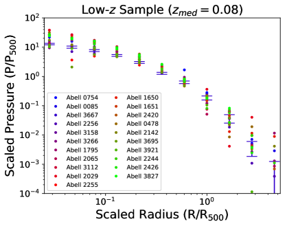
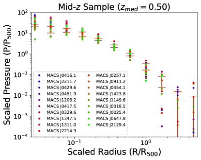
Refer to caption — Figure 1: Joint X-ray/SZ effect scaled pressure deprojections for all 40 galaxy clusters in our sample, with the low- $z$ objects plotted on the top and the mid- $z$ objects plotted on the bottom. The dots indicate the best-fit value at each radius for each galaxy cluster. The square root of the diagonal elements of the covariance matrix are shown as error bars for a single galaxy cluster in each plot to provide an indication of the typical measurement uncertainty.

We simultaneously fit the X-ray and SZ effect data using a generalized least squares algorithm to obtain the best-fit values of the P_i and $\mathcal{R}$ (Markwardt, 2009). In the case of the X-ray data, the deprojected ICM density and temperature profiles are compared directly with the pressure profile model. To compare with the SZ data, the three-dimensional pressure model is projected along one dimension to obtain a two-dimensional $y$ -map. As part of this projection, relativistic corrections to the SZ effect are included based on the X-ray temperature profile using SZpack (Chluba et al., 2012, 2013). For Planck, this projected model is convolved with the PSF shape, which is assumed to be Gaussian with a FWHM of 10′. An analogous PSF convolution is also used for Bolocam, based on a Gaussian with a FWHM of 58″. In addition, the filtering effects of the Bolocam data processing, which are described by a two-dimensional transfer function included in the public data release, are applied to the projected model. The deprojections for all 40 galaxy clusters in our sample are shown in Figure 1, with numerical values provided in Table 4 of the Appendix.

In performing these fits, we assume the noise is accurately modeled by a diagonal covariance matrix, primarily because it is not possible to quantitatively estimate the off-diagonal elements of the Bolocam covariance matrix (for more details, see Wan et al., 2021). To test for biases due to this assumption, we generate a set of mock datasets by inserting a galaxy cluster with a known pressure profile into random noise realizations of the various datasets. For Bolocam, 1000 such noise realizations are included with the public data release, while for Planck they were generated from a combination of the homogeneous and inhomogeneous noise spectra associated with those data. Samples from the Markov chain Monte Carlo employed to analyze the X-ray data were used to create noise realizations associated with the Chandra and ROSAT data. For each of these samples, the values of M₅₀₀ and R₅₀₀ were also extracted and used to scale the $\textrm{P}_{i}$ and $\textrm{R}_{i}$ values, thus ensuring that uncertainties on our mass estimates are properly accounted for in our overall error budget.

A total of 100 mocks were then analyzed in an identical manner to the observed data, including the assumption of a diagonal covariance matrix, and the fitted pressure profiles were compared with the known input profiles. We find no evidence for a radial trend in the ratio of fitted to input pressure, and we also find no evidence for an on-average non-zero difference between the two values. The standard deviation of the ratio between the fitted and true pressure value is 0.022 for the low- $z$ sample and 0.033 for the mid- $z$ sample. These numbers represent the fluctuations in the recovered pressure profiles due to our fitting procedure. Compared to the measurement noise and calibration uncertainties on the pressure values, these systematic variations due to fitting are a factor of approximately 5–10 smaller. Since these fluctuations are negligible to our overall error budget, and they also do not produce a measurable bias that might appear in ensemble averages, we do not account for them in our analysis.

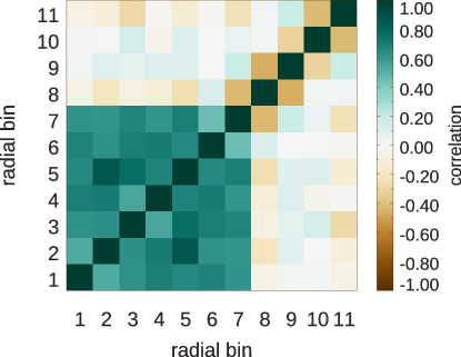
In addition to using our fits to the mocks to search for biases, we also use them to characterize the noise covariance matrix associated with the joint X-ray/SZ effect pressure deprojection values P_i. In general, the off-diagonal elements of this covariance matrix are significant. For the inner radial bins, which are largely constrained by the X-ray data, the P_i are strongly positively correlated due to the constant multiplicative factor $\mathcal{R}$ included in the fits to account for uncertainties in the X-ray temperature calibration. In the outer radial bins, which are largely constrained by the SZ effect data, there is typically a large negative correlation between adjacent P_i. This arises from the course angular resolution of the data, whereby the observed maps are largely unchanged when an upward fluctuation in one pressure bin is compensated by downward fluctuations in the adjacent bins. A typical example of the correlation values of the covariance matrix is given in Figure 2.

Because of the typically large correlations in the noise covariance matrices for each galaxy cluster, the matrices contain small eigenvalues that can lead to unstable fits (e.g. Michael, 1994; Yoon et al., 2012). In order to use these individual pressure profiles to obtain the ensemble fits described in Sections 4 and 5, we thus need to address this problem. Several solutions to obtain more stable fits from such covariance matrices have been proposed, including setting all of the off-diagonal elements to zero (Bae et al., 2010). For this analysis, we choose to employ the cutoff method, also known as the singular value decomposition method, in order to obtain covariance matrices that produce more stable fits (Bhattacharya et al., 1999; Gamiz et al., 2011; Yoon et al., 2012). Specifically, we compute the eigenvalues of the covariance matrices for all 40 galaxy clusters. For each object, we then search for sufficiently small eigenvalues, quantified as those smaller than $10^{-4}$ of the maximum eigenvalue. The eigenmodes associated with these small values are removed, and the covariance matrix is reformed based on the remaining eigenmodes and eigenvalues. This trimming occurs in a total of 5 galaxy clusters, and involves 1–2 eigenmodes per object. Thus, only a small fraction of our sample is impacted by this procedure.

4 Ensemble Mean Scaled Pressure Profiles

4.1 Analysis Procedure

Using the set of individual pressure deprojections described in Section 3, which have all been computed in units of scaled pressure relative to P₅₀₀ at a set of common scaled radii relative to R₅₀₀, we constrain the ensemble mean profile for each of the two subsamples (low- $z$ and mid- $z$ ). To determine the mean profile, we use the publicly available LRGS software package from Mantz (2016), which also returns the covariance matrix of the intrinsic scatter about the mean profile (i.e., $\Sigma_{\textrm{int}}(\textrm{R}_{i},\textrm{R}_{i})$ ). We perform these fits in a two-step process.

First, an initial estimate of the mean profile is obtained directly from the scaled pressure deprojections. Using this initial estimate, we compute a single multiplicative normalization factor N_l for the deprojection of each individual galaxy cluster $l$ . Specifically, we first compute

\mathcal{P}_{i}^{l}=\mathrm{P}_{i}^{l}/\langle\mathrm{P}_{i}^{l}\rangle

(3)

where $\langle\mathrm{P}_{i}^{l}\rangle$ is the mean profile. Next, we compute

\textrm{N}_{l}=[\vec{\mathcal{P}^{l}}]^{\mathrm{T}}[C^{l}]^{-1}\vec{\mathcal{P}^{l}}

(4)

where $C^{l}$ is the weighted covariance matrix associated with $\vec{\mathrm{P}^{l}}$ , and the vector represents the set of radial bins $i$ . Then, we fit the N_l as a function of $\tilde{\textrm{M}}_{l}=\textrm{M}_{500,l}/\langle\textrm{M}_{500}\rangle$ , where $\langle\textrm{M}_{500}\rangle$ is the mean mass of the given subsample and the assumed functional form is N ${}_{l}=\tilde{\textrm{M}}_{l}^{\alpha_{\textrm{\tiny{M}}}}$ . We find consistent values for the power law exponent in both the low- $z$ and mid- $z$ subsamples, with $\alpha_{\textrm{\tiny{M}}}=-0.30\pm 0.19$ and $-0.14\pm 0.18$ , respectively. These values indicate that our data favor, at low significance, a slightly shallower dependence of P₅₀₀ with mass compared to Equation 2 (i.e., closer to M₅₀₀^1/2 rather than M₅₀₀^2/3). Given the narrow redshift range of each subsample, we do not attempt to fit an analogous relation as a function of $E(z)$ .

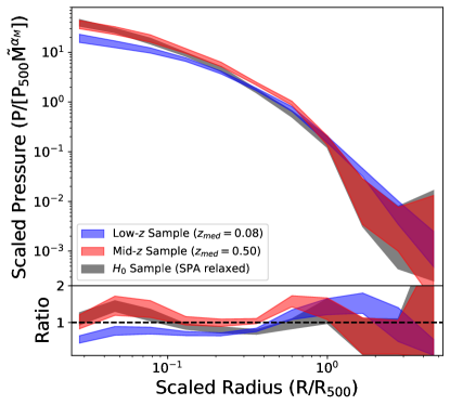
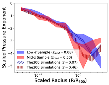
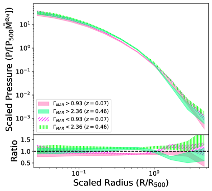
Second, using the fitted value of $\alpha_{\textrm{\tiny{M}}}$ for each subsample, we rescale the pressure values of each individual deprojection. We then refit for the ensemble mean profile, along with the intrinsic scatter about that mean profile. Compared to the initial fit (with $\alpha_{\textrm{\tiny{M}}}=0$ ), there is a slightly smaller intrinsic scatter but essentially no change to the ensemble mean profile. A summary of the results is given in Figure 3, with numerical values provided in Tables 6 and 7 in the Appendix. For the bins at R ${}_{i}\leq 1.7$ R₅₀₀ the individual P_i are generally measured at high significance, with a SNR of at least 3 when estimated from the diagonal elements of the covariance matrix. The same is true for the ensemble mean profiles, where the SNR is comparable to the individual cluster values due to the large intrinsic scatter. In the two outermost bins, the SNR is typically lower, corresponding to $\simeq 2$ for the low- $z$ sample and to $\simeq 1$ for the mid- $z$ sample for both the individual profiles and the mean profiles. We note that the Planck data for the mid- $z$ sample are in general noisier than for the low- $z$ sample, which is the primary reason for the difference in uncertainties on the mean profiles at the largest radii. The scaled pressure profiles for both samples monotonically steepen with increasing radius, corresponding to an effective power law exponent of $\sim-0.5$ at the smallest radii and $\sim-3$ to $\sim-5$ at the largest radii (see Section 4.3). Finally, in both the low- $z$ and mid- $z$ samples the fractional intrinsic scatter decreases from near unity in the smallest radial bin to a minimum of $\sim 0.2$ near 0.5R₅₀₀. Beyond that radius the fractional intrinsic scatter increases, reaching a value of $\gtrsim 2$ in the largest radial bin.

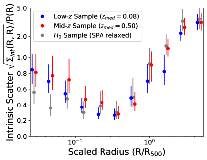
4.2 Comparison of the low- $z$ , mid- $z$ , and $H_{0}$ Samples

From Figure 3, it is clear that there is a systematic difference in the mean scaled pressure profile shape between the low- $z$ and mid- $z$ samples. Specifically, at radii smaller than approximately 0.6R₅₀₀, the mean scaled pressure is significantly higher in the mid- $z$ sample compared to the low- $z$ sample. The trend reverses near 2R₅₀₀, with a higher mean scaled pressure in the low- $z$ sample, although at modest statistical significance. The intrinsic scatter about the mean profile is consistent at all radii for the two samples.

We have also repeated the same analysis using the highly relaxed sample of galaxy clusters from Wan et al. (2021, hereafter the $H_{0}$ sample) to search for any obvious trends with dynamical state. The $H_{0}$ sample contains 14 objects distributed approximately uniformly between $0.08\leq z\leq 0.54$ with a median redshift of $z=0.33$ . The masses range from $4.7\leq\textrm{M}_{500}\leq 17.4\times 10^{14}$ M_☉ with a median mass of $8.5\times 10^{14}$ M_☉. Thus, based on both mass and redshift, the $H_{0}$ sample is almost perfectly intermediate to the low- $z$ and mid- $z$ samples.

At the smallest and largest radii, corresponding to $\textrm{R}\lesssim 0.2$ R₅₀₀ and $\textrm{R}\gtrsim 1$ R₅₀₀, we find that the mean scaled pressure profiles of the $H_{0}$ and mid- $z$ samples are in good agreement. At intermediate radii, the mean scaled pressure profile of the low- $z$ sample more closely traces that of the $H_{0}$ sample. Thus, rather than falling in between the mean scaled pressure profiles of the low- $z$ and mid- $z$ samples as would be expected purely due to differences in redshift and mass, the mean profile from the $H_{0}$ sample is instead much more sharply peaked at small radii. We attribute this to: 1) the uniform presence of cool cores in the $H_{0}$ sample, which are known to enhance the central pressure (e.g., Arnaud et al., 2010; Sayers et al., 2013b), and 2) the center determined from the procedure in Section 2.2 is likely to be coincident with the X-ray peak for cool-core systems, thus retaining a higher central pressure for those galaxy clusters.

We find that the fractional intrinsic scatter about the mean scaled pressure profile is somewhat smaller in the $H_{0}$ sample for the innermost radial bins, although at low statistical significance. Such a difference is expected, again due to the uniformity of cool cores within this sample which reduces the relative spread among the population in the central regions.

4.3 Comparison with The Three Hundred Simulations

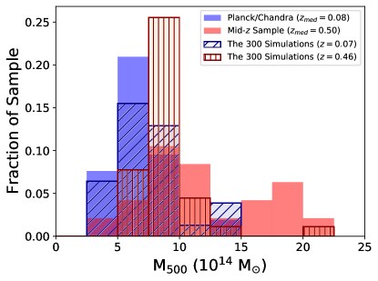
To better understand if the observed difference between the mean scaled pressure profiles in the low- $z$ and mid- $z$ samples is due to evolution, mass scaling, and/or dynamical state, we also performed our analysis on a set of scaled pressure profiles obtained from The Three Hundred simulations (Cui et al., 2018). A range of redshift snapshots for 324 galaxy clusters are available in these simulations, and we have selected the two that most closely match the median redshifts of our low- $z$ and mid- $z$ samples, which are at $z=0.07$ and $z=0.46$ . Within each snapshot, we would ideally like to apply a simple and quantitative selection based on the X-ray luminosity in order to obtain a large statistically representative set of galaxy clusters matching the properties of the observed samples. However, such a selection is unlikely to yield the best set of matched galaxy clusters. First, the mid- $z$ sample contains numerous additional selections beyond a simple luminosity threshold that are not straightforward to include, such as the timing between when subsamples of MACS clusters were known in the literature and when Bolocam conducted its observations. Furthermore, our observed samples were selected from the full sky, and include the most massive and thus rare objects. While the underlying dark-matter only simulation used to obtain The Three Hundred sample is large, with a comoving side length of 1 $h^{-1}$ Gpc, it is unclear if a selection based on X-ray luminosity from this volume will provide the best individual matches to the observed mid- $z$ systems.

Instead, within each snapshot, we select the three simulated galaxy clusters most similar in mass to each observed galaxy cluster, removing duplicates. Three matches was chosen as a reasonable compromise between obtaining sufficiently large samples (which motivates a larger number of matches) while still retaining a good representation of the population statistics (which motivates a smaller number of matches). From these candidate samples, we then remove all of the objects that contain two or more distinct sub-clusters, indicating they are in a pre-merger phase (i.e., analogous to the removal of Abell 399/401 from the observational sample). Next, we determine which objects are relaxed or disturbed based on the criteria defined by Cui et al. (2018), and randomly remove galaxy clusters until the fraction of both types approximately match the observed samples. Following these cuts, we were left with a samples of 31 $z=0.07$ and 36 $z=0.46$ simulated galaxy clusters. With the exception of the mass distribution of the simulated sample at $z=0.46$ , where there were not enough high mass objects to match the observed mid- $z$ sample, these simulated samples are well matched to the properties of the observed samples (i.e., redshift, mass, and dynamical state, see Figure 4 and Table 2).

Table 2: Observed and Simulated Samples

Sample	N ${}_{\textrm{clus}}$	N ${}_{\textrm{r}}$	N ${}_{\textrm{d}}$	$\langle$ M₅₀₀ $\rangle$	$\langle$ $z$ $\rangle$
This Work (low- $z$ )	21	02	04	06.1 ${}^{\textrm{a}}$	0.08
Arnaud et al. (2010)	31	10	12	02.6 ${}^{\textrm{a}}$	0.12
Bourdin et al. (2017)	61	22	39	07.2 ${}^{\textrm{a}}$	0.15
Ghirardini et al. (2019)	12	04	08	05.7 ${}^{\textrm{a}}$	0.06
The300 (low- $z$ Matched)	31	03	06	06.7 ${}^{\textrm{a}}$	0.07
This Work (mid- $z$ )	19	4	3	10.6 ${}^{\textrm{a}}$	0.50
McDonald et al. (2014)	40	19	21	05.5 ${}^{\textrm{a}}$	0.46
Bourdin et al. (2017)	23	—	—	07.9 ${}^{\textrm{a}}$	0.56
Ghirardini et al. (2017)	15	08	07	09.7 ${}^{\textrm{a}}$	0.45
The300 (mid- $z$ Matched)	36	08	06	08.2 ${}^{\textrm{a}}$	0.46

Note. — Studies of ensemble mean scaled pressure profiles from galaxy cluster samples with similar masses and redshifts to those in our low- $z$ (top) and mid- $z$ (bottom) samples, along with the samples selected from The Three Hundred simulations. The total number of galaxy clusters, the number of relaxed and disturbed galaxy clusters, median mass, and median redshift of each sample is listed. For studies from the literature, unless otherwise noted by the authors, we consider the objects listed as cool cores to be relaxed and the non cool cores to be disturbed.

${}^{\textrm{a}}$ Since no masses were provided in Ghirardini et al. (2017), we compute them from the values of M ${}_{\textrm{gas,500}}$ given in Amodeo et al. (2016) assuming a gas mass fraction of 0.125 (Mantz et al., 2016b)

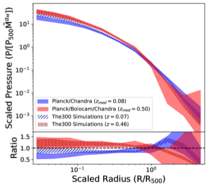
To determine the pressure profiles of the simulated galaxy clusters, we use the center positions obtained from the Amiga Halo Finder algorithm (AHF, Knollmann & Knebe, 2009). These centers correspond to the location of the maximum in total density, and are thus likely to be more similar to the observed centers obtained from the procedure in Section 2.2 than the location of the ICM peak. From the initial fits, we find $\alpha_{\textrm{\tiny{M}}}=-0.39\pm 0.15$ and $-0.26\pm 0.16$ , for the $z=0.07$ and $z=0.46$ samples, in good agreement with the values obtained from the observational data. The shape of the mean scaled pressure profiles recovered from the matched The Three Hundred samples are shown in the top panel of Figure 5, and numerical values are provided in Tables 8 and 9 of the Appendix. Overall, the agreement with the observed data is excellent, with the possible exception of the core region of the low- $z$ sample, indicating that the simulations accurately reproduce the measured differences between the low- $z$ and mid- $z$ samples. Furthermore, in regards to the uncertainties on the ensemble mean profiles in Figure 5, we note that the intrinsic scatter is larger than the measurement uncertainties for the observed data at all radii other than the outermost bins. It thus dominates the overall uncertainty on the mean profile, resulting in similar constraints for both the observed data and the (perfectly known) simulated data.

In Figure 6 we show the effective power law exponent of the scaled pressure versus radius for the observed and matched simulated samples, which are generally in excellent agreement. In the central region the exponent is near $-0.5$ , steepening to approximately $-4$ near the maximum radii included in our analysis. At both redshifts, The Three Hundred simulations suggest a significant steepening of the profile between the radial bins at 1.7R₅₀₀ and 2.8R₅₀₀ with a minimum exponent of less than $-4$ . The statistical significance of this minimum is approximately $5\sigma$ for the low- $z$ sample and $2\sigma$ for the mid- $z$ sample. The observed data also indicate a minimum exponent of less than $-4$ at large radii, between the 2.8R₅₀₀ and 4.6R₅₀₀ radial bins for the low- $z$ sample and between the 1.0R₅₀₀ and 1.7R₅₀₀ radial bins for the mid- $z$ sample. The statistical significance of these minima is lower than for the simulated samples, approximately $2\sigma$ for the low- $z$ sample and $1\sigma$ for the mid- $z$ sample.

Recent results have used SZ data to similarly probe large radius features in the pressure profile, including Hurier et al. (2019, for a single massive cluster at low- $z$ ), Pratt et al. (2021, for a sample of 10 group-size objects in the local universe), and Anbajagane et al. (2022, for a sample of 516 clusters detected in the South Pole Telescope SPT-SZ survey). The latter study, along with Baxter et al. (2021), also included simulated clusters from The Three Hundred.

In mass, redshift, and sample size, the Anbajagane et al. (2022) result is the only one directly comparable to our analysis, and so we consider that study in more detail. From The Three Hundred simulations, they find a minimum exponent near R₂₀₀ (which is $\sim 1.5$ R₅₀₀), corresponding to slightly smaller radii than the minimum in our analysis. They also find a minimum exponent in the observed data at a similar radius, in good agreement with the location of the minimum we find in the observed mid- $z$ sample but at smaller radii than in the observed low- $z$ sample. The overall agreement between our analyses is thus quite good, particularly given the differences in analysis technique (our work considers deprojected pressure profiles and the effect of intrinsic scatter while Anbajagane et al. 2022 considers projected pressure profiles) and overall sample characteristics (the Anbajagane et al. 2022 sample is most similar in mass to our low- $z$ sample and most similar in redshift to our mid- $z$ sample). In addition, the coarse radial binning of our analysis prevents an accurate determination of the location of the minimum exponent, which may also be contributing to some of the differences in our results. We further note that, while the underlying physical cause of this minimum exponent is not well understood, Anbajagane et al. (2022) suggest it may be due to shock-induced thermal non-equilibrium between electrons and ions (see, e.g. Avestruz et al., 2015).

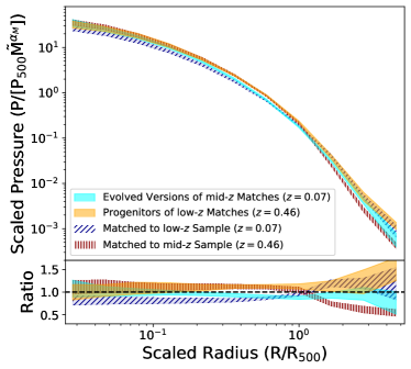
Given the good agreement between the observed and simulated mean scaled pressure profiles, we defined three additional samples from The Three Hundred to better understand the underlying cause of the difference between the low- $z$ and mid- $z$ samples. First, in order to best isolate the impact of evolution between the observed samples, we repeated our analysis for the $z=0.07$ counterparts of the matched $z=0.46$ galaxy clusters (i.e., the same set of objects were extracted from the simulations at two different redshifts). A similar analysis was also performed on the $z=0.46$ counterparts of the matched $z=0.07$ galaxy clusters. The results are shown in the top left panel of Figure 7, and indicate: 1) there is a clear trend of decreasing scaled pressure with decreasing redshift at intermediate radii, with the low- $z$ and mid- $z$ profiles separated by 2–3 times the width of 68 per cent confidence regions; 2) there are hints of a similar trend at small radii near the core, although all of the profiles overlap within the 68 per cent confidence regions; 3) at large radii there is evidence of increasing scaled pressure with decreasing redshift in the mid- $z$ -matched galaxy clusters, which are separated by approximately 2 times the width of the 68 per cent confidence regions, but there is no such trend in the low- $z$ -matched objects.

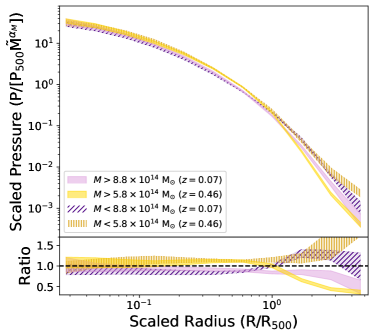
Next, to best isolate the impact of mass, we considered the full set of The Three Hundred galaxy clusters at both $z=0.07$ and $z=0.46$ selected either as a match to the low- $z$ or mid- $z$ samples (i.e., 67 objects). We then split this set of galaxy clusters into two samples based on the overall median mass at each snapshot, which is equal to $8.8\times 10^{14}$ M_☉ at $z=0.07$ and $5.8\times 10^{14}$ M_☉ at $z=0.46$ . The results are shown in the top right panel of Figure 7, and indicate: 1) there is no significant trend in the mean scaled pressure profile shape based on mass within R₅₀₀, where the profiles at a given redshift snapshot overlap within the 68 per cent confidence regions at all radii; 2) there is strong trend of increasing scaled pressure with decreasing mass outside of that radius, with the profiles separated by approximately 2–3 times the width of the 68 per cent confidence region at $z=0.07$ and by even more than that amount at $z=0.46$ ; 3) the trend of decreasing scaled pressure with decreasing redshift at intermediate radii noted in the previous paragraph is again reproduced here with a separation of approximately 3 times the width of the 68 per cent region.

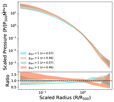
Finally, to best isolate the impact of dynamical state, we again split the full set of The Three Hundred galaxy clusters at $z=0.07$ and $z=0.46$ based on the value of the dynamical state parameter $\chi_{\textrm{dyn}}$ defined by De Luca et al. (2021). In brief, this parameter is computed as a weighted quadratic sum of the ratio between the thermal and potential energy $\eta$ , the offset between the galaxy cluster center and the center of mass $\Delta_{\textrm{r}}$ , and the mass fraction of all the sub-halos in the galaxy cluster $f_{\textrm{s}}$ , all of which were evaluated within R₂₀₀. The set of objects with $\chi_{\textrm{dyn}}>1$ were defined to be the more dynamically relaxed samples, and the set of objects with $\chi_{\textrm{dyn}}<1$ were defined to be the less dynamically relaxed samples. The results are shown in the bottom panel of Figure 7, and indicate: 1) a higher mean scaled pressure at small radii in the more dynamically relaxed sample, with the profiles separated by approximately 2 times the width of the 68 per cent confidence regions; 2) at larger radii there is less difference in the profiles based on dynamical state, although the more relaxed samples have slightly lower pressure in both redshift snapshots; 3) again, the trend of decreasing scaled pressure with decreasing redshift at intermediate radii is evident, with the profiles separated by approximately twice the width of the 68 per cent confidence regions.

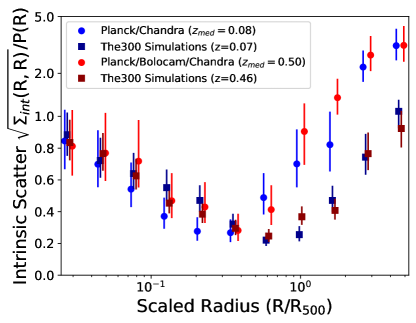
The lower panel of Figure 5 compares the fractional intrinsic scatter about the mean scaled pressure profiles for the observations and The Three Hundred. While the simulations show the same basic radial trend as the observed data (i.e., a minimum scatter near 0.5R₅₀₀), the fractional intrinsic scatter in The Three Hundred samples is lower than the observed data at large radii. This could, for example, indicate that the observed data have a wider range of accretion histories, although we note the potential for systematics. One such possibility is the presence of unmodeled noise in the observed data at large angular scales, for example due to galactic dust emission or primary CMB anisotropies, which is then interpreted as additional scatter in our fits. Astrophysical systematics in the observed data are another possibility. For instance, the presence of unrelated structures along the LOS that were not flagged by our analysis procedure would also enhance the intrinsic scatter recovered in our fits. However, given that the low- $z$ sample is far more sensitive to such projection effects due to their larger angular extent, we would expect this systematic to produce a difference between the low- $z$ and mid- $z$ samples, which is not observed.

4.4 Comparison to Previous Observations

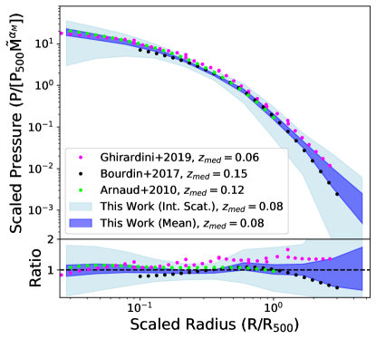
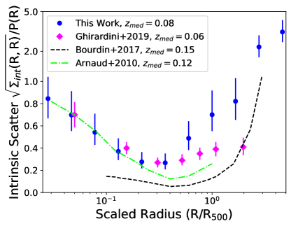
Three previous analyses have measured ensemble mean scaled pressure profiles and the associated intrinsic scatter for galaxy cluster samples with similar mass and redshift distributions to our low- $z$ sample (Arnaud et al., 2010; Bourdin et al., 2017; Ghirardini et al., 2019, , see Table 2). As shown in the top panel of Figure 8, both the overall shape and the normalization of the mean profiles found in these works are in excellent agreement with our analysis. The level of consistency is remarkable, particularly given the range of analysis techniques and observational datasets. There is also generally good agreement in the fractional scatter about the mean profile at small and intermediate radii (lower panel of Figure 8), although our observed results are somewhat higher at large radii and Bourdin et al. (2017) find a lower scatter at all radii.

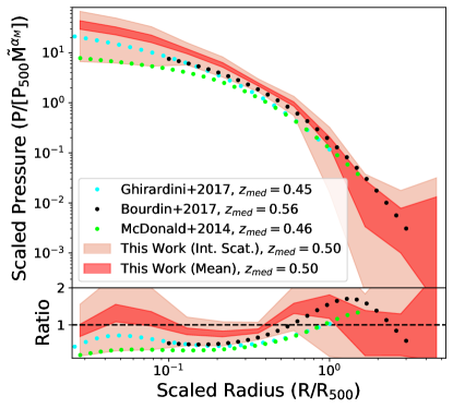
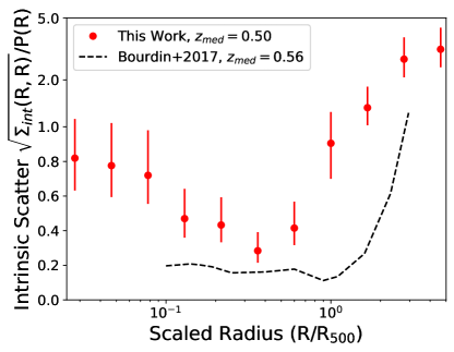
There are also three previous analyses that have constrained ensemble mean scaled pressure profiles using samples well matched in mass and redshift to our mid- $z$ sample (McDonald et al., 2014; Bourdin et al., 2017; Ghirardini et al., 2017, , see Figure 9). While the agreement is fairly good near R₅₀₀, there is a noticeable divergence at smaller radii. Our work finds the highest mean scaled pressure at those radii, while McDonald et al. (2014) obtains much lower values and the other two studies are approximately half way between. The trend approximately correlates with the mean mass of the samples, and so that is a possible explanation for the difference. Given that the differences are most pronounced near the core, the centering algorithms used in these works may also play a role (e.g., McDonald et al., 2014, used a centroid determined from an annulus at 250–500 kpc, which could result in a lower central scaled pressure). Alternatively, these discrepancies could be due to the distribution of dynamical states within the samples. While no obvious differences exist based on the relative fractions of relaxed and disturbed systems listed in Table 2, we note that each analysis used different criteria for identifying such systems. For instance, when a uniform set of criteria are used, there is an observed difference in cool core fraction between SZ- and X-ray-selected samples (Rossetti et al., 2017; Andrade-Santos et al., 2017; Lovisari et al., 2017). The McDonald et al. (2014) sample is purely SZ-selected, which could thus result in a lower cool core fraction and correspondingly lower inner scaled pressure. In contrast, our mid- $z$ sample is X-ray-selected from MACS, which is known to have a significant bias towards cool core systems (Rossetti et al., 2017). The samples of Bourdin et al. (2017) and Ghirardini et al. (2017) have less defined selections that are likely somewhat intermediate. Therefore, it is possible that at least some of the difference between these observed profiles is due to dynamical state. Only Bourdin et al. (2017) measured the fractional intrinsic scatter as part of their analysis. As with the lower $z$ samples, they again find a similar overall trend with radius as our analysis, but with significantly smaller values.

5 gNFW Fits

Particularly for recent analyses involving SZ effect data, the gNFW parameterization proposed by Nagai et al. (2007) has become standard in describing ICM pressure profiles. Specifically,

\textrm{P}(x)=\textrm{P}_{0}x^{-\gamma}(1+x^{\alpha})^{-(\beta-\gamma)/\alpha},

(5)

where $\textrm{P}_{0}$ is the pressure normalization; $\gamma$ , $\alpha$ , and $\beta$ primarily describe the power law exponent at small, intermediate, and large radii; and $x=c_{500}(\textrm{R}/\textrm{R}_{500})$ is the scaled radial coordinate with concentration $c_{500}$ . As originally noted by Nagai et al. (2007), degeneracies between the five parameters in the model often prevent meaningful constraints when all are varied (see also Battaglia et al., 2012a). Thus, to describe the individual galaxy cluster pressure profiles obtained from our deprojection procedure in Section 3, we first considered gNFW fits that varied every possible permutation of $\textrm{P}_{0}$ and either two or three of the other four parameters. Due to the strong degeneracies between parameters, we found from an initial set of sparsely sampled fits that the fitted shape over the radial range constrained by the data, along with the fit quality, was similar regardless of the total number of varied parameters as long as one of them was $\beta$ . Based on these test fits, we chose to vary $\textrm{P}_{0}$ , $\alpha$ , and $\beta$ in our final fits because that combination produced the best fit quality among the three-parameter fits (with $c_{500}=1.4$ and $\gamma=0.3$ ). Numerical values for all of the fitted parameters are provided in Table 5 of the Appendix.

Using our full sample of 40 galaxy clusters, we then searched for trends in the values of the fitted parameters according to the parameterizations used by Battaglia et al. (2012a), with

	$\displaystyle\log_{10}(\textrm{A})=\log_{10}(\textrm{A}_{0})+a_{\textrm{m}}\log_{10}(\textrm{M}_{500}/10^{15})$
	$\displaystyle+a_{z}\log_{10}(1+z)$		(6)

and the values of $a_{\textrm{m}}$ and $a_{z}$ describing the mass and redshift dependence of the parameter. For each fitted gNFW parameter, we determined the values of A₀, $a_{\textrm{m}}$ , and $a_{z}$ , along with the fractional intrinsic cluster-to-cluster scatter in A, using a grid search. The derived values are given in Table 3.

Table 3: gNFW Fit Parameters

Parameter	$\log_{10}($ A ${}_{0})$	a ${}_{\textrm{m}}$	a_z	$\sigma_{\textrm{int}}(\log_{10}(\textrm{A}))$
Observational Sample
P₀	$\phantom{-}0.74\pm 0.17$	$-0.27\pm 0.45$	$\phantom{-}2.10\pm 1.29$	$0.52\pm 0.10$
$\alpha$	$\phantom{-}0.12\pm 0.11$	$\phantom{-}0.12\pm 0.29$	$-0.41\pm 0.83$	$0.24\pm 0.05$
$\beta$	$\phantom{-}0.74\pm 0.04$	$\phantom{-}0.15\pm 0.10$	$\phantom{-}0.02\pm 0.28$	$0.10\pm 0.02$
$\left[\textrm{P}_{0}\alpha\right]_{\parallel}$	$-0.63\pm 0.20$	$\phantom{-}0.30\pm 0.53$	$-2.09\pm 1.52$	$0.56\pm 0.11$
$\left[\textrm{P}_{0}\alpha\right]_{\perp}$	$\phantom{-}0.41\pm 0.03$	$\phantom{-}0.00\pm 0.08$	$\phantom{-}0.48\pm 0.24$	$0.08\pm 0.02$
The Three Hundred
P₀	$\phantom{-}0.77\pm 0.16$	$-0.04\pm 0.59$	$\phantom{-}1.70\pm 1.14$	$0.63\pm 0.08$
$\alpha$	$\phantom{-}0.12\pm 0.10$	$\phantom{-}0.03\pm 0.35$	$-0.24\pm 0.68$	$0.29\pm 0.04$
$\beta$	$\phantom{-}0.71\pm 0.02$	$\phantom{-}0.19\pm 0.07$	$\phantom{-}0.27\pm 0.13$	$0.07\pm 0.01$
$\left[\textrm{P}_{0}\alpha\right]_{\parallel}$	$-0.66\pm 0.19$	$\phantom{-}0.51\pm 0.69$	$-1.65\pm 1.32$	$0.69\pm 0.09$
$\left[\textrm{P}_{0}\alpha\right]_{\perp}$	$\phantom{-}0.42\pm 0.02$	$\phantom{-}0.01\pm 0.08$	$\phantom{-}0.47\pm 0.16$	$0.08\pm 0.01$
Battaglia et al. (2012a)
P₀	$\phantom{-}1.16$	$\phantom{-}0.27$	$-1.50$
$\alpha$	$-0.05$	$-0.05$	$\phantom{-}0.50$
$\beta$	$\phantom{-}0.73$	$\phantom{-}0.08$	$\phantom{-}0.25$
$\left[\textrm{P}_{0}\alpha\right]_{\parallel}$	$-1.08$	$-0.26$	$\phantom{-}1.57$
$\left[\textrm{P}_{0}\alpha\right]_{\perp}$	$\phantom{-}0.43$	$\phantom{-}0.06$	$-0.15$

Note. — Generalized NFW fit parameters from our observational sample, The Three Hundred, and Battaglia et al. (2012a).

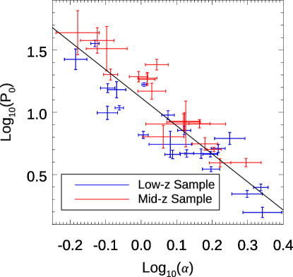
While we find that the parameters in Equation 6 are precisely measured for $\beta$ , the parameters associated with P₀ and $\alpha$ are relatively poorly constrained. This is because, even when only varying three of the gNFW parameters, there is still a significant degeneracy between P₀ and $\alpha$ , as illustrated in Figure 10. To better explore this issue, we have therefore derived two new parameters based on a linear fit to $\log_{10}(\textrm{P}_{0})$ versus $\log_{10}(\alpha)$ . One is parallel to this linear fit, with

\log_{10}(\left[\textrm{P}_{0}\alpha\right]_{\parallel})=-0.91\log_{10}(\textrm{P}_{0})+0.41\log_{10}(\alpha),

(7)

and the other is perpendicular, with

\log_{10}(\left[\textrm{P}_{0}\alpha\right]_{\perp})=0.41\log_{10}(\textrm{P}_{0})+0.91\log_{10}(\alpha).

(8)

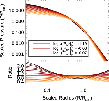
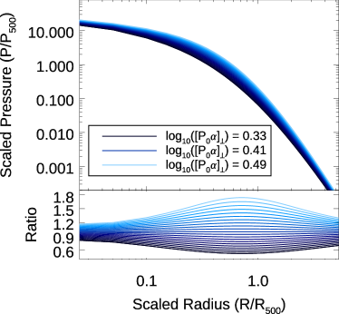
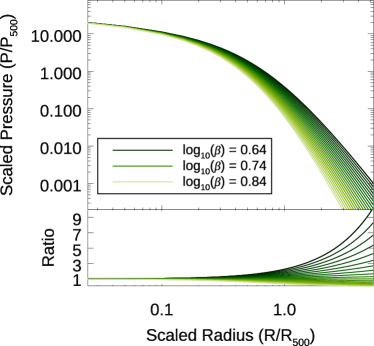
Figure 11 shows how the overall gNFW profile shape depends on these these parallel and perpendicular components, and illustrates that this decomposition of the gNFW parameters is useful to interpreting the results. Specifically, the small radius behavior is almost entirely governed by $\left[\textrm{P}_{0}\alpha\right]_{\parallel}$ , the intermediate radius behavior is almost entirely governed by $\left[\textrm{P}_{0}\alpha\right]_{\perp}$ , and the large radius behavior is almost entirely governed by $\beta$ . In Figure 13 of the Appendix we show plots of all the parameter pairs, and a an additional small degeneracy between $\left[\textrm{P}_{0}\alpha\right]_{\perp}$ and $\beta$ is evident. Unlike the P₀– $\alpha$ degeneracy, accounting for this small degeneracy does not significantly improve the scatter in the transformed parameters compared to the original parameters, and so we do not include an additional parameter transformation in our analysis.

As expected, the results presented in Table 3 and Figure 11 are consistent with what we found from the ensemble mean profiles in Section 4. In particular, both $\left[\textrm{P}_{0}\alpha\right]_{\parallel}$ and $\left[\textrm{P}_{0}\alpha\right]_{\perp}$ have measurable evolution that results in on-average higher scaled pressure values at small and intermediate radii with increasing redshift. In addition, $\beta$ has a measurable mass dependence that indicates lower scaled pressure values with increasing mass. Thus, the general mass and redshift trends that were inferred in Section 4 based on various subsamples from The Three Hundred are confirmed in these gNFW fits. Furthermore, these three parameters suggest a fractional intrinsic scatter in the scaled pressure that is of order unity at small radii, approximately 50 per cent at intermediate radii, and several times larger than unity at large radii.

For comparison, we also fit gNFW profiles to the set of simulated clusters selected from The Three Hundred, and performed an identical analysis to constrain the mass and redshift dependence of the fitted parameters (see Table 3). Again, as expected, the results are largely consistent with what we find for the observational sample, suggesting good agreement between the observations and simulations. We note that, while the values of a_z for $\beta$ are consistent given the measurement uncertainties, The Three Hundred find a non-zero value indicative of decreasing scaled pressure with increasing redshift at large radii.

In addition, we also rescaled the fitted gNFW parameters from Battaglia et al. (2012a) for comparison. This involved generating a grid of pressure profiles in mass and redshift based on the best-fit values given in Table 1 of that work for the “AGN Feedback $\Delta=500$ ” case using their Equation 10. These profiles were then refit using our parameterization, with the results given in Table 3. Their value of $\beta$ , including its mass and redshift dependence, is consistent with what we find in our analysis, suggesting good consistency in the scaled pressure values at large radii. The same is generally true for $\left[\textrm{P}_{0}\alpha\right]_{\perp}$ , where we find nearly identical values for A₀ and a_m. However, in contrast to the evolution found in our analysis, Battaglia et al. (2012a) find a much weaker (and opposite) redshift dependence, indicating minor differences in the scaled pressure at intermediate radii between our analyses. Finally, Battaglia et al. (2012a) find a lower normalization for $\left[\textrm{P}_{0}\alpha\right]_{\parallel}$ and a positive rather than negative value for the associated a_z. This indicates that they find higher scaled pressures at small radii that decrease rather than increase with redshift. However, as noted in Section 4, our observed trend with redshift appears to be largely due to selection effects with regard to dynamical state, and so we caution that no general conclusions should be drawn based on this comparison between our analyses at small radii.

6 Discussion

The ensemble mean scaled pressure profiles we obtain for our low- $z$ and mid- $z$ samples are generally in good agreement with The Three Hundred simulations and previous observational studies. One exception is the profiles obtained by previous observational studies at small to intermediate radii at mid- $z$ , which are lower than those from our analysis. While the origin of this difference is unclear, we speculate it may be due to the choice of centering algorithm and/or the distribution of dynamical states within the various samples used in these analyses. Similarly, we generally find good agreement in the fractional intrinsic scatter about these mean profiles, although our analysis suggests a higher scatter at large radii compared to both The Three Hundred and previous observational studies. We also find generally good agreement for the mass and redshift dependence of our measured profiles compared with the parametric gNFW fits provided by Battaglia et al. (2012a) based on their simulations, where again the only notable discrepancy appears at smaller radii where selection effects appear to play a dominant role.

We measure a significant difference in the mean scaled pressure profiles between the low- $z$ and mid- $z$ samples, and we use The Three Hundred simulations to better understand these differences. At small radii, dynamical state has the largest impact, with more relaxed systems having higher scaled pressure. While subdominant to dynamical state, there are also modest indications of evolution playing a role at small radii, with higher redshift systems having higher scaled pressure. At intermediate radii, we find that evolution is the primary driver, resulting in higher mean scaled pressure with increasing redshift. However, dynamical state may also play a role here, given that cool core systems can have higher pressures extending well beyond the core and the MACS X-ray selection of the mid- $z$ sample has a significant bias towards such systems. At large radii, mass has the most influence on the mean scaled pressure, with lower mass systems having higher scaled pressure. In addition, there are also some indications of evolution at large radii, with higher redshift systems having lower scaled pressure. In order to facilitate a mapping of our measured mean scaled pressure profiles to any combination of redshift and mass that is well constrained by our study, corresponding to approximately 0.05 $\leq z\leq$ 0.60 and $4\times 10^{14}$ M_☉ $\leq\textrm{M}_{500}\leq 30\times 10^{14}$ M_☉, we provide a set of gNFW parameter values in Table 3.

To better understand the physical processes responsible for the evolution and mass dependence we find in our analysis, we consider the results from a range of previous simulations. For instance, the pressure profile at large radii is expected to steepen with increasing mass accretion rates due to halo contraction during accretion and the further penetration of the accretion shocks required to thermalize the new material (Battaglia et al., 2012b; Diemer & Kravtsov, 2014; Lau et al., 2015; Planelles et al., 2017; Aung et al., 2021; Diemer, 2022). Higher mass accretion rates should also reduce the overall thermalization fraction of the ICM, and thus its pressure, particularly at large radii, as suggested by recent measurements from Sereno et al. (2021). Given that the mass accretion rate is enhanced in higher mass and/or higher redshift galaxy clusters (e.g., Diemer & Kravtsov, 2014; Battaglia et al., 2015), those systems are expected to have lower scaled pressure at large radii.

To test this expectation, we determined the mass accretion rate for all of simulated The Three Hundred galaxy clusters matched to the observed samples in Section 4.3 and plotted in Figure 7 according to the formalism of Diemer (2017) with

\Gamma_{\textrm{MAR}}=\frac{\log_{10}(\textrm{M}_{0})-\log_{10}(\textrm{M}_{1})}{\log_{10}(1+z_{1})-\log_{10}(1+z_{0})},

(9)

where M and $z$ are mass and redshift at epochs 0 and 1. We then determined the mean pressure profile for samples selected to be above or below the median value of $\Gamma_{\textrm{MAR}}$ at both $z=0.07$ and $z=0.46$ , with the results shown in Figure 12. We find the following: 1) within each redshift snapshot, the higher $\Gamma_{\textrm{MAR}}$ sample has lower pressure and thus a steeper profile beyond R₅₀₀; 2) the on-average value of $\Gamma_{\textrm{MAR}}$ is a factor of 2.5 higher in the $z=0.46$ sample than the $z=0.07$ sample, yet there is no significant difference in the profiles outside of R₅₀₀; 3) the higher redshift (and thus higher $\Gamma_{\textrm{MAR}}$ ) samples do have higher pressure at $\textrm{R}\lesssim\textrm{R}_{500}$ , indicating a steeper profile in those systems at intermediate radii. Thus, while we do find trends of steeper pressure profiles at both intermediate and large radii in higher $\Gamma_{\textrm{MAR}}$ systems, there does not appear to be a simple mapping between $\Gamma_{\textrm{MAR}}$ and profile shape, with redshift and potentially other characteristics also playing a role.

As another example, the relative impact of AGN feedback is expected to be larger in low mass galaxy clusters, resulting in more gas being ejected from the central regions to larger radii during outbursts (Battaglia et al., 2010; McCarthy et al., 2011; Battaglia et al., 2012b; Le Brun et al., 2015; Barnes et al., 2017; Truong et al., 2018; Henden et al., 2020). While this effect is most likely to be relevant in group-scale objects with lower masses than the systems in our study, some simulations indicate there may still be observable differences in low-to-moderate mass galaxy clusters. Thus, our observed flattening of the scaled pressure profiles in lower mass systems at both small and large radii may by caused in part by AGN. Other mechanisms, such as star formation, are also expected to have a larger fractional impact on lower mass systems, producing similar trends in the scaled pressure profile (Battaglia et al., 2012b; Henden et al., 2020). There are also indications of evolution in the mean scaled pressure profile due to the increasing prevalence of AGN at higher redshift, primarily resulting in an enhanced level of thermal pressure at large radii (Battaglia et al., 2012b).

Taken as a whole, our observed mass and redshift trends on the mean scaled pressure profile are broadly consistent with expectations from simulations. We find that differences in mass accretion rate are a significant contributor to these trends, although these differences are unable to fully explain the trends. For instance, while the effects are generally expected to be minimal for the high mass galaxy clusters typical of our study, feedback from AGN and other relevant feedback processes also produce mass and redshift trends in broad agreement with our observations.

Considering the intrinsic scatter rather than the mean scaled pressure profile, we find no measurable difference between the low- $z$ and mid- $z$ samples. The matched samples from The Three Hundred also show consistent scatter at all radii, further suggesting that the scatter is largely independent of population statistics. While most results from simulations have focused more on the impact of physical process on the mean shape rather than the scatter, Planelles et al. (2017) examined the issue in some detail. For instance, they noted a significant increase in scatter at small radii when AGN feedback was included, although the scatter at larger radii was not sensitive to the included physics. Furthermore, the increased clumpiness associated with higher mass accretion rates (e.g., at higher redshift) was found to increase the scatter. If such trends do exist, then they appear to be below our measurement precision.

Sayers and Mantz were supported by the National Aeronautics and Space Administration under Grant No. 80NSSC18K0920 issued through the ROSES 2017 Astrophysics Data Analysis Program. Wan was supported by a Robert L. Blinkenberg Caltech Summer Undergraduate Research Fellowship and the Kavli Institute for Particle Astrophysics and Cosmology. Allen and Morris were supported by the U.S. Department of Energy under contract number DE-AC02-76SF00515.

Appendix A Individual and Ensemble Mean Galaxy Cluster Scaled Pressure Profiles

This appendix includes tabulated values for the individual galaxy cluster pressure profile deprojections and gNFW fits. It also includes tabulated values for the ensemble pressure profile deprojections for the observed and simulated data.

Table 4: Scaled Pressure Deprojections

R/R₅₀₀	0.028	0.047	0.078	0.13	0.22	0.36	0.60	1.0	1.7	2.8	4.6
Abell 0754	2.18E+01	1.10E+01	9.22E+00	8.94E+00	4.47E+00	2.25E+00	1.67E+00	2.81E-01	3.61E-02	5.17E-03	$\leq$ 4.5E-03
Abell 0085	1.62E+01	1.57E+01	9.80E+00	5.77E+00	3.62E+00	1.56E+00	8.19E-01	2.54E-01	6.32E-02	7.07E-03	2.88E-03
Abell 3667	1.28E+01	1.01E+01	7.67E+00	5.21E+00	3.01E+00	1.28E+00	6.33E-01	1.86E-01	3.74E-02	3.93E-03	$\leq$ 1.2E-03
Abell 2256	1.12E+01	7.05E+00	6.18E+00	5.17E+00	3.13E+00	1.56E+00	5.21E-01	1.21E-01	1.85E-02	1.09E-03	3.88E-04
Abell 3158	—	1.20E+01	1.04E+01	6.90E+00	3.70E+00	1.70E+00	7.74E-01	2.30E-01	6.61E-02	4.47E-03	$\leq$ 1.2E-03
Abell 3266	9.45E+00	9.47E+00	5.58E+00	4.90E+00	3.66E+00	1.66E+00	9.40E-01	1.59E-01	3.63E-02	2.68E-03	1.30E-03
Abell 1795	2.46E+01	1.77E+01	1.28E+01	7.19E+00	3.75E+00	1.50E+00	6.36E-01	1.21E-01	2.34E-02	4.61E-03	1.16E-02
Abell 2065	1.40E+01	1.18E+01	8.87E+00	6.10E+00	3.80E+00	2.14E+00	8.52E-01	5.13E-02	4.00E-02	$\leq$ 6.5E-03	8.61E-04
Abell 3112	3.80E+01	2.67E+01	1.71E+01	1.04E+01	5.09E+00	2.24E+00	6.50E-01	7.55E-02	6.08E-02	9.71E-03	2.31E-07
Abell 2029	3.81E+01	2.52E+01	1.56E+01	8.97E+00	3.98E+00	1.61E+00	5.64E-01	3.64E-01	4.13E-03	4.03E-02	$\leq$ 5.5E-04
Abell 2255	—	3.63E+00	4.94E+00	4.80E+00	2.44E+00	1.83E+00	8.03E-01	2.10E-01	5.94E-02	$\leq$ 1.6E-03	$\leq$ 2.8E-03
Abell 1650	2.63E+01	2.19E+01	1.49E+01	8.41E+00	4.76E+00	1.87E+00	6.85E-01	2.19E-01	1.30E-02	1.15E-02	8.92E-03
Abell 1651	2.71E+01	2.02E+01	1.35E+01	9.79E+00	4.71E+00	1.98E+00	7.41E-01	1.48E-01	4.64E-02	7.58E-05	$\leq$ 5.4E-03
Abell 2420	2.64E+01	2.02E+01	1.46E+01	9.54E+00	5.82E+00	2.59E+00	7.99E-01	1.77E-01	2.73E-02	4.13E-03	6.91E-04
Abell 0478	3.15E+01	2.10E+01	1.60E+01	8.24E+00	3.77E+00	1.37E+00	4.67E-01	1.94E-01	8.54E-03	1.91E-02	$\leq$ 4.2E-03
Abell 2142	1.74E+01	1.19E+01	8.48E+00	5.88E+00	3.12E+00	1.38E+00	6.52E-01	2.18E-01	2.22E-02	3.33E-03	4.14E-03
Abell 3695	1.20E+01	2.09E+00	5.58E+00	4.67E+00	2.87E+00	1.39E+00	4.95E-01	2.00E-01	3.76E-02	9.77E-03	6.90E-05
Abell 3921	1.03E+01	8.98E+00	9.76E+00	5.45E+00	3.62E+00	1.85E+00	6.46E-01	1.05E-01	7.18E-02	1.15E-04	$\leq$ 3.9E-03
Abell 2244	2.74E+01	1.96E+01	1.61E+01	8.58E+00	4.27E+00	1.71E+00	6.44E-01	8.10E-02	5.67E-02	9.44E-03	1.11E-03
Abell 2426	2.66E+01	2.03E+01	1.27E+01	9.82E+00	5.53E+00	2.53E+00	8.30E-01	1.77E-01	2.66E-02	2.46E-03	$\leq$ 9.1E-04
Abell 3827	2.42E+01	1.90E+01	1.60E+01	8.93E+00	4.99E+00	2.59E+00	7.55E-01	1.80E-01	8.23E-02	3.74E-03	$\leq$ 3.1E-03
MACS J0416.1	3.27E+01	1.94E+01	1.24E+01	8.88E+00	7.58E+00	2.93E+00	1.37E+00	6.80E-02	$\leq$ 1.8E-02	$\leq$ 4.8E-03	$\leq$ 4.0E-03
MACS J2211.7	7.63E+01	4.24E+01	3.05E+01	1.34E+01	6.07E+00	2.56E+00	7.97E-01	7.26E-02	1.16E-06	1.50E-02	1.67E-04
MACS J0429.6	6.74E+01	3.12E+01	2.83E+01	1.14E+01	8.76E+00	3.01E+00	1.33E+00	3.78E-01	$\leq$ 3.8E-02	$\leq$ 6.7E-03	$\leq$ 1.7E-02
MACS J0451.9	3.04E+01	3.74E+01	1.40E+01	1.19E+01	3.38E+00	1.90E+00	7.42E-01	8.34E-02	1.95E-05	2.54E-02	2.35E-02
MACS J1206.2	3.33E+01	2.85E+01	1.71E+01	1.03E+01	4.82E+00	2.34E+00	7.99E-01	2.17E-01	3.30E-04	1.03E-02	2.41E-04
MACS J0417.5	1.93E+01	7.19E+00	1.31E+01	6.80E+00	3.85E+00	2.04E+00	8.21E-01	1.06E-01	$\leq$ 1.1E-02	1.90E-02	7.08E-04
MACS J0329.6	6.07E+01	5.85E+01	2.91E+01	1.73E+01	8.35E+00	2.32E+00	1.25E+00	3.46E-01	$\leq$ 3.2E-02	$\leq$ 1.7E-02	$\leq$ 1.2E-02
MACS J1347.5	6.07E+01	4.57E+01	3.88E+01	1.53E+01	8.63E+00	2.60E+00	7.12E-01	1.26E-01	2.85E-05	$\leq$ 4.4E-05	4.23E-02
MACS J1311.0	5.09E+01	4.91E+01	3.48E+01	1.68E+01	9.16E+00	4.17E+00	1.28E+00	4.85E-01	1.60E-02	5.53E-04	3.80E-02
MACS J2214.9	2.77E+01	2.23E+01	1.73E+01	1.08E+01	5.43E+00	2.21E+00	9.76E-01	1.79E-01	1.44E-03	$\leq$ 4.5E-03	$\leq$ 3.2E-03
MACS J0257.1	3.96E+01	2.46E+01	1.64E+01	8.75E+00	6.52E+00	2.39E+00	1.40E+00	1.41E-01	$\leq$ 2.0E-02	3.81E-04	8.63E-03
MACS J0911.2	2.43E+01	1.62E+01	1.43E+01	9.38E+00	5.15E+00	2.44E+00	9.63E-01	2.66E-01	5.43E-02	6.63E-03	1.56E-03
MACS J0454.1	1.64E+01	1.81E+01	1.57E+01	1.01E+01	6.09E+00	2.64E+00	9.79E-01	1.31E-01	$\leq$ 1.3E-02	$\leq$ 3.5E-03	3.73E-02
MACS J1423.8	5.84E+01	4.53E+01	2.54E+01	1.26E+01	7.11E+00	2.25E+00	9.78E-01	7.23E-02	$\leq$ 4.1E-01	$\leq$ 4.2E-03	$\leq$ 8.5E-03
MACS J1149.6	1.49E+01	1.22E+01	8.91E+00	5.93E+00	3.37E+00	1.53E+00	5.22E-01	1.24E-01	2.09E-02	2.53E-03	2.13E-04
MACS J0018.5	2.06E+01	1.62E+01	1.06E+01	6.93E+00	3.93E+00	2.15E+00	7.39E-01	1.85E-01	1.20E-02	5.53E-03	2.85E-03
MACS J0025.4	5.16E+00	6.78E+00	8.17E+00	5.04E+00	4.93E+00	2.54E+00	9.89E-01	1.13E-01	$\leq$ 4.2E-04	$\leq$ 5.2E-05	$\leq$ 5.6E-06
MACS J0647.8	4.98E+01	2.81E+01	2.35E+01	1.33E+01	7.43E+00	2.97E+00	1.64E+00	3.26E-01	$\leq$ 1.8E-02	$\leq$ 5.8E-03	$\leq$ 5.3E-03
MACS J2129.4	3.11E+01	4.16E+01	2.17E+01	1.61E+01	5.02E+00	1.87E+00	1.14E+00	5.19E-02	$\leq$ 1.9E-02	$\leq$ 5.6E-03	$\leq$ 3.7E-03

Note. — Scaled pressure deprojections for all of the observed galaxy clusters. Due to strong degeneracies between the values, error estimates are omitted from this table. Missing values at small radii are interior to the radius of the innermost Chandra/ROSAT X-ray deprojection bin. Upper limits (at 68 per cent confidence) are given for pressure values at large radii that are consistent with zero.

Table 5: gNFW Fit Parameters

Cluster	P₀	$\alpha$	$\beta$	$\gamma$	$c_{500}$
Abell 0754	004.60	1.57	4.43	0.30	1.40
Abell 0085	026.64	0.65	4.16	0.30	1.40
Abell 3667	004.67	1.34	5.62	0.30	1.40
Abell 2256	002.49	2.17	6.57	0.30	1.40
Abell 3158	004.58	1.23	4.27	0.30	1.40
Abell 3266	003.49	1.57	4.71	0.30	1.40
Abell 1795	009.89	0.80	4.30	0.30	1.40
Abell 2065	004.66	1.47	5.51	0.30	1.40
Abell 3112	010.85	0.87	5.18	0.30	1.40
Abell 2029	016.69	1.02	6.05	0.30	1.40
Abell 2255	002.21	1.99	4.42	0.30	1.40
Abell 1650	015.18	0.85	4.81	0.30	1.40
Abell 1651	007.15	1.32	6.32	0.30	1.40
Abell 2420	006.17	1.78	6.99	0.30	1.40
Abell 0478	035.70	0.74	5.24	0.30	1.40
Abell 2142	006.58	1.01	4.51	0.30	1.40
Abell 3695	001.57	2.19	4.60	0.30	1.40
Abell 3921	005.12	1.65	7.07	0.30	1.40
Abell 2244	015.64	0.80	4.67	0.30	1.40
Abell 2426	005.53	1.21	4.80	0.30	1.40
Abell 3827	009.50	1.19	5.91	0.30	1.40
MACS J0416.1	008.33	1.32	5.41	0.30	1.40
MACS J2211.7	018.35	1.04	6.66	0.30	1.40
MACS J0429.6	014.77	1.07	5.01	0.30	1.40
MACS J0451.9	204.07	0.40	3.94	0.30	1.40
MACS J1206.2	020.08	0.82	5.01	0.30	1.40
MACS J0417.5	005.03	1.60	6.04	0.30	1.40
MACS J0329.6	043.58	0.66	4.57	0.30	1.40
MACS J1347.5	024.12	1.11	8.05	0.30	1.40
MACS J1311.0	037.74	0.75	4.41	0.30	1.40
MACS J2214.9	008.05	1.34	5.86	0.30	1.40
MACS J0257.1	008.47	1.32	5.82	0.30	1.40
MACS J0911.2	006.35	1.15	4.26	0.30	1.40
MACS J0454.1	008.09	1.46	6.69	0.30	1.40
MACS J1423.8	019.33	0.98	4.94	0.30	1.40
MACS J1149.6	003.93	1.67	6.20	0.30	1.40
MACS J0018.5	005.57	1.51	6.36	0.30	1.40
MACS J0025.4	003.95	1.97	6.23	0.30	1.40
MACS J0647.8	018.78	1.04	5.50	0.30	1.40
MACS J2129.4	032.42	0.80	5.71	0.30	1.40

Note. — Generalized NFW parameters for all of the observed galaxy clusters. Due to the strong degeneracies between parameters, error estimates are omitted from this table.

{rotatetable*}

Table 6: low-

z

Observational Sample

R/R₅₀₀	0.028	0.047	0.078	0.13	0.22	0.36	0.60	1.0	1.7	2.8	4.6
Mean Pressure
	1.94E+01	1.47E+01	1.10E+01	7.16E+00	3.91E+00	1.79E+00	7.29E-01	1.79E-01	3.87E-02	6.92E-03	1.48E-03
Measurement Covariance Matrix
0.028	1.50E+01	8.41E+00	4.72E+00	2.09E+00	6.89E-01	8.19E-02	-5.97E-02	2.15E-02	-1.35E-02	9.08E-03	5.91E-04
0.047	—	5.92E+00	3.22E+00	1.33E+00	4.68E-01	6.29E-02	-4.76E-02	1.05E-02	-5.76E-03	5.09E-03	4.92E-04
0.078	—	—	2.00E+00	7.66E-01	2.55E-01	3.58E-02	-3.84E-02	3.01E-03	-2.03E-03	2.83E-03	2.02E-04
0.13	—	—	—	3.90E-01	1.34E-01	3.22E-02	8.96E-04	3.27E-03	-1.40E-03	1.05E-03	-1.68E-05
0.22	—	—	—	—	6.41E-02	1.91E-02	2.08E-03	-3.93E-05	-4.05E-04	1.80E-04	-1.32E-06
0.36	—	—	—	—	—	1.25E-02	3.48E-03	-3.91E-04	1.59E-04	-7.23E-05	-3.75E-05
0.6	—	—	—	—	—	—	7.29E-03	6.66E-04	4.71E-05	-6.65E-05	-1.04E-05
1.0	—	—	—	—	—	—	—	8.69E-04	-7.34E-05	6.75E-05	-8.83E-07
1.7	—	—	—	—	—	—	—	—	5.67E-05	-1.31E-05	-2.68E-06
2.8	—	—	—	—	—	—	—	—	—	1.28E-05	-1.16E-07
4.6	—	—	—	—	—	—	—	—	—	—	1.19E-06
Intrinsic Scatter Covariance Matrix
0.028	2.69E+02	1.50E+02	8.34E+01	3.74E+01	1.22E+01	1.42E+00	-9.24E-01	3.83E-01	-2.38E-01	1.60E-01	7.51E-03
0.047	—	1.05E+02	5.69E+01	2.36E+01	8.25E+00	1.04E+00	-7.50E-01	1.96E-01	-1.01E-01	9.03E-02	6.91E-03
0.078	—	—	3.53E+01	1.36E+01	4.49E+00	6.03E-01	-6.12E-01	6.07E-02	-3.80E-02	5.02E-02	2.60E-03
0.13	—	—	—	7.05E+00	2.40E+00	5.60E-01	2.45E-02	5.82E-02	-2.42E-02	1.85E-02	-6.24E-04
0.22	—	—	—	—	1.17E+00	3.37E-01	3.65E-02	1.72E-03	-7.00E-03	3.27E-03	-1.17E-04
0.36	—	—	—	—	—	2.30E-01	5.99E-02	-6.09E-03	2.64E-03	-1.26E-03	-6.42E-04
0.6	—	—	—	—	—	—	1.27E-01	1.07E-02	8.90E-04	-1.11E-03	-1.61E-04
1.0	—	—	—	—	—	—	—	1.57E-02	-1.25E-03	1.19E-03	-1.48E-05
1.7	—	—	—	—	—	—	—	—	1.01E-03	-2.30E-04	-4.36E-05
2.8	—	—	—	—	—	—	—	—	—	2.35E-04	-2.86E-06
4.6	—	—	—	—	—	—	—	—	—	—	2.13E-05

Note. — Ensemble mean pressure (in units of P₅₀₀) and associated covariance (in units of P₅₀₀²).

{rotatetable*}

Table 7: mid-

z

Observational Sample

R/R₅₀₀	0.028	0.047	0.078	0.13	0.22	0.36	0.60	1.0	1.7	2.8	4.6
Mean Pressure
	3.68E+01	2.78E+01	1.93E+01	1.07E+01	5.76E+00	2.33E+00	9.48E-01	1.71E-01	1.59E-02	4.77E-03	7.65E-03
Measurement Covariance Matrix
0.028	5.77E+01	3.23E+01	2.30E+01	6.63E+00	3.33E+00	4.68E-01	1.23E-01	1.73E-02	-1.75E-02	-2.56E-04	3.59E-03
0.047	—	3.03E+01	1.57E+01	6.39E+00	1.87E+00	6.53E-02	4.68E-03	-1.56E-04	-1.33E-02	-1.90E-03	9.09E-03
0.078	—	—	1.24E+01	3.85E+00	1.74E+00	2.79E-01	2.24E-02	1.63E-02	-7.55E-03	-1.25E-03	9.32E-03
0.13	—	—	—	1.67E+00	4.69E-01	4.98E-02	1.85E-02	1.21E-03	-3.03E-03	-4.67E-04	2.53E-03
0.22	—	—	—	—	3.96E-01	6.69E-02	2.54E-02	6.25E-03	-1.37E-03	-1.03E-03	1.47E-03
0.36	—	—	—	—	—	2.85E-02	4.67E-03	2.30E-03	-1.66E-04	-4.64E-05	3.90E-04
0.6	—	—	—	—	—	—	1.01E-02	8.81E-04	-2.43E-04	-1.18E-04	-1.32E-04
1.0	—	—	—	—	—	—	—	1.58E-03	4.21E-05	-3.53E-05	-4.83E-06
1.7	—	—	—	—	—	—	—	—	3.08E-05	-9.41E-07	-6.21E-06
2.8	—	—	—	—	—	—	—	—	—	1.09E-05	-1.42E-06
4.6	—	—	—	—	—	—	—	—	—	—	3.88E-05
Intrinsic Scatter Covariance Matrix
0.028	8.94E+02	4.84E+02	3.53E+02	9.86E+01	5.03E+01	7.09E+00	1.80E+00	2.78E-01	-2.51E-01	-2.18E-03	4.78E-02
0.047	—	4.56E+02	2.34E+02	9.62E+01	2.71E+01	1.08E+00	1.09E-01	1.42E-02	-1.88E-01	-2.45E-02	1.28E-01
0.078	—	—	1.91E+02	5.82E+01	2.65E+01	4.13E+00	3.49E-01	2.30E-01	-1.05E-01	-1.88E-02	1.29E-01
0.13	—	—	—	2.53E+01	6.83E+00	7.39E-01	2.69E-01	2.03E-02	-4.22E-02	-6.51E-03	3.53E-02
0.22	—	—	—	—	6.10E+00	1.01E+00	3.64E-01	8.53E-02	-1.93E-02	-1.50E-02	2.05E-02
0.36	—	—	—	—	—	4.32E-01	6.93E-02	3.26E-02	-2.27E-03	-6.85E-04	5.13E-03
0.6	—	—	—	—	—	—	1.53E-01	1.28E-02	-3.38E-03	-1.61E-03	-1.80E-03
1.0	—	—	—	—	—	—	—	2.40E-02	5.75E-04	-4.99E-04	-1.17E-04
1.7	—	—	—	—	—	—	—	—	4.62E-04	-1.32E-05	-7.63E-05
2.8	—	—	—	—	—	—	—	—	—	1.64E-04	-2.38E-05
4.6	—	—	—	—	—	—	—	—	—	—	5.76E-04

Note. — Ensemble mean pressure (in units of P₅₀₀) and associated covariance (in units of P₅₀₀²).

{rotatetable*}

Table 8: low-

z

Matched Sample from The Three Hundred

R/R₅₀₀	0.028	0.047	0.078	0.13	0.22	0.36	0.60	1.0	1.7	2.8	4.6
Mean Pressure
	2.49E+01	1.94E+01	1.32E+01	7.92E+00	4.11E+00	1.81E+00	6.63E-01	1.87E-01	3.73E-02	4.62E-03	5.73E-04
Measurement Covariance Matrix
0.028	1.73E+01	1.06E+01	5.89E+00	2.70E+00	9.79E-01	2.43E-01	7.64E-03	-1.88E-02	-1.13E-03	8.69E-04	-3.59E-05
0.047	—	7.03E+00	4.11E+00	1.93E+00	7.01E-01	1.75E-01	8.12E-03	-1.12E-02	-5.14E-04	5.51E-04	-1.83E-05
0.078	—	—	2.54E+00	1.25E+00	4.75E-01	1.19E-01	7.60E-03	-6.54E-03	-5.00E-04	2.86E-04	-1.13E-05
0.13	—	—	—	6.80E-01	2.80E-01	7.12E-02	5.20E-03	-3.29E-03	-4.70E-04	6.92E-05	-4.62E-06
0.22	—	—	—	—	1.33E-01	3.62E-02	3.16E-03	-1.55E-03	-3.74E-04	-7.51E-06	-2.24E-06
0.36	—	—	—	—	—	1.21E-02	1.69E-03	-4.66E-04	-1.46E-04	-6.64E-06	-2.19E-07
0.6	—	—	—	—	—	—	7.57E-04	-1.26E-05	-3.55E-05	-4.64E-06	-8.80E-07
1.0	—	—	—	—	—	—	—	7.96E-05	1.34E-05	-7.01E-07	-1.24E-07
1.7	—	—	—	—	—	—	—	—	1.07E-05	7.50E-07	3.58E-08
2.8	—	—	—	—	—	—	—	—	—	4.15E-07	2.59E-08
4.6	—	—	—	—	—	—	—	—	—	—	1.32E-08
Intrinsic Scatter Covariance Matrix
0.028	4.86E+02	2.96E+02	1.64E+02	7.46E+01	2.68E+01	6.64E+00	2.28E-01	-5.14E-01	-3.71E-02	2.32E-02	-1.12E-03
0.047	—	1.96E+02	1.14E+02	5.32E+01	1.91E+01	4.78E+00	2.38E-01	-3.03E-01	-1.78E-02	1.47E-02	-5.20E-04
0.078	—	—	7.09E+01	3.48E+01	1.31E+01	3.30E+00	2.17E-01	-1.77E-01	-1.62E-02	7.49E-03	-3.03E-04
0.13	—	—	—	1.90E+01	7.86E+00	1.99E+00	1.47E-01	-9.04E-02	-1.45E-02	1.67E-03	-1.18E-04
0.22	—	—	—	—	3.74E+00	1.02E+00	8.92E-02	-4.24E-02	-1.11E-02	-2.55E-04	-5.56E-05
0.36	—	—	—	—	—	3.39E-01	4.73E-02	-1.28E-02	-4.14E-03	-1.80E-04	-1.27E-06
0.6	—	—	—	—	—	—	2.14E-02	-3.08E-04	-9.82E-04	-1.22E-04	-2.34E-05
1.0	—	—	—	—	—	—	—	2.28E-03	3.79E-04	-1.88E-05	-3.71E-06
1.7	—	—	—	—	—	—	—	—	3.09E-04	2.10E-05	1.12E-06
2.8	—	—	—	—	—	—	—	—	—	1.18E-05	7.21E-07
4.6	—	—	—	—	—	—	—	—	—	—	3.86E-07

Note. — Ensemble mean pressure (in units of P₅₀₀) and associated covariance (in units of P₅₀₀²).

{rotatetable*}

Table 9: mid-

z

Matched Sample from The Three Hundred

R/R₅₀₀	0.028	0.047	0.078	0.13	0.22	0.36	0.60	1.0	1.7	2.8	4.6
Mean Pressure
	3.72E+01	2.89E+01	1.90E+01	1.11E+01	5.77E+00	2.47E+00	8.60E-01	2.14E-01	2.49E-02	2.54E-03	4.20E-04
Measurement Covariance Matrix
0.028	2.80E+01	1.90E+01	8.89E+00	3.50E+00	1.20E+00	2.70E-01	-2.10E-02	-1.88E-02	-2.24E-03	-2.04E-04	-8.92E-05
0.047	—	1.40E+01	7.05E+00	2.82E+00	9.87E-01	2.12E-01	-1.38E-02	-1.35E-02	-1.40E-03	-1.26E-04	-4.69E-05
0.078	—	—	4.04E+00	1.66E+00	6.26E-01	1.39E-01	-6.70E-03	-9.02E-03	-8.74E-04	-8.22E-05	-2.24E-05
0.13	—	—	—	7.34E-01	2.97E-01	7.06E-02	-2.04E-03	-3.97E-03	-4.56E-04	-3.43E-05	-7.31E-06
0.22	—	—	—	—	1.44E-01	4.09E-02	8.89E-04	-2.21E-03	-2.79E-04	-3.09E-05	-1.66E-06
0.36	—	—	—	—	—	1.57E-02	1.89E-03	-5.98E-04	-1.01E-04	-1.41E-05	-8.57E-08
0.6	—	—	—	—	—	—	1.30E-03	9.68E-05	-9.03E-06	-1.50E-06	-1.67E-07
1.0	—	—	—	—	—	—	—	1.82E-04	1.24E-05	8.23E-07	-8.54E-08
1.7	—	—	—	—	—	—	—	—	3.06E-06	1.67E-07	-6.76E-09
2.8	—	—	—	—	—	—	—	—	—	1.11E-07	9.21E-09
4.6	—	—	—	—	—	—	—	—	—	—	4.33E-09
Intrinsic Scatter Covariance Matrix
0.028	9.68E+02	6.59E+02	3.10E+02	1.22E+02	4.15E+01	9.40E+00	-6.25E-01	-6.53E-01	-7.44E-02	-6.81E-03	-3.03E-03
0.047	—	4.89E+02	2.47E+02	9.80E+01	3.43E+01	7.34E+00	-4.15E-01	-4.64E-01	-4.58E-02	-4.43E-03	-1.64E-03
0.078	—	—	1.41E+02	5.76E+01	2.16E+01	4.74E+00	-2.29E-01	-3.02E-01	-2.82E-02	-2.84E-03	-7.99E-04
0.13	—	—	—	2.55E+01	1.02E+01	2.40E+00	-7.09E-02	-1.33E-01	-1.48E-02	-1.20E-03	-2.66E-04
0.22	—	—	—	—	4.91E+00	1.38E+00	2.93E-02	-7.29E-02	-9.16E-03	-1.05E-03	-6.41E-05
0.36	—	—	—	—	—	5.31E-01	6.38E-02	-1.99E-02	-3.41E-03	-4.77E-04	-4.41E-06
0.6	—	—	—	—	—	—	4.48E-02	3.29E-03	-3.40E-04	-5.30E-05	-5.93E-06
1.0	—	—	—	—	—	—	—	6.18E-03	4.00E-04	2.48E-05	-2.94E-06
1.7	—	—	—	—	—	—	—	—	1.03E-04	5.77E-06	-2.04E-07
2.8	—	—	—	—	—	—	—	—	—	3.78E-06	3.12E-07
4.6	—	—	—	—	—	—	—	—	—	—	1.50E-07

Note. — Ensemble mean pressure (in units of P₅₀₀) and associated covariance (in units of P₅₀₀²).

Appendix B Fitted gNFW Parameters

This appendix includes plots of the fitted gNFW profiles for the observed galaxy clusters.

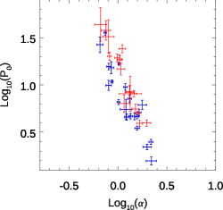
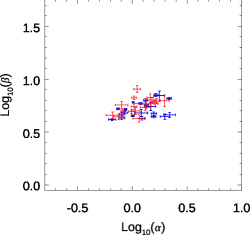
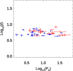
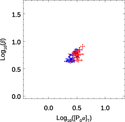
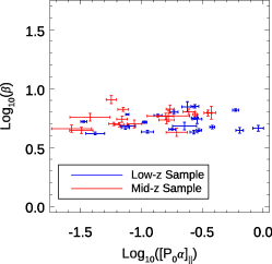
References

Adam et al. (2017) Adam, R., Bartalucci, I., Pratt, G. W., et al. 2017, A&A, 598, A115, doi: 10.1051/0004-6361/201629182
Allen et al. (2011) Allen, S. W., Evrard, A. E., & Mantz, A. B. 2011, ARA&A, 49, 409, doi: 10.1146/annurev-astro-081710-102514
Amodeo et al. (2016) Amodeo, S., Ettori, S., Capasso, R., & Sereno, M. 2016, A&A, 590, A126, doi: 10.1051/0004-6361/201527630
Anbajagane et al. (2022) Anbajagane, D., Chang, C., Jain, B., et al. 2022, MNRAS, 514, 1645, doi: 10.1093/mnras/stac1376
Andrade-Santos et al. (2017) Andrade-Santos, F., Jones, C., Forman, W. R., et al. 2017, ApJ, 843, 76, doi: 10.3847/1538-4357/aa7461
Arnaud et al. (2010) Arnaud, M., Pratt, G. W., Piffaretti, R., et al. 2010, A&A, 517, A92, doi: 10.1051/0004-6361/200913416
Aung et al. (2021) Aung, H., Nagai, D., & Lau, E. T. 2021, MNRAS, 508, 2071, doi: 10.1093/mnras/stab2598
Avestruz et al. (2015) Avestruz, C., Nagai, D., Lau, E. T., & Nelson, K. 2015, ApJ, 808, 176, doi: 10.1088/0004-637X/808/2/176
Bae et al. (2010) Bae, T., Jang, Y.-C., Jung, C., et al. 2010, Phys. Rev. D, 82, 114509, doi: 10.1103/PhysRevD.82.114509
Barnes et al. (2017) Barnes, D. J., Kay, S. T., Henson, M. A., et al. 2017, MNRAS, 465, 213, doi: 10.1093/mnras/stw2722
Bartalucci et al. (2017) Bartalucci, I., Arnaud, M., Pratt, G. W., et al. 2017, A&A, 598, A61, doi: 10.1051/0004-6361/201629509
Battaglia et al. (2012a) Battaglia, N., Bond, J. R., Pfrommer, C., & Sievers, J. L. 2012a, ApJ, 758, 75, doi: 10.1088/0004-637X/758/2/75
Battaglia et al. (2012b) —. 2012b, ApJ, 758, 74, doi: 10.1088/0004-637X/758/2/74
Battaglia et al. (2015) —. 2015, ApJ, 806, 43, doi: 10.1088/0004-637X/806/1/43
Battaglia et al. (2010) Battaglia, N., Bond, J. R., Pfrommer, C., Sievers, J. L., & Sijacki, D. 2010, ApJ, 725, 91, doi: 10.1088/0004-637X/725/1/91
Baxter et al. (2021) Baxter, E. J., Adhikari, S., Vega-Ferrero, J., et al. 2021, MNRAS, 508, 1777, doi: 10.1093/mnras/stab2720
Bhattacharya et al. (1999) Bhattacharya, T., Chandrasekharan, S., Gupta, R., Lee, W., & Sharpe, S. 1999, Physics Letters B, 461, 79, doi: 10.1016/S0370-2693(99)00796-0
Böhringer et al. (2004) Böhringer, H., Schuecker, P., Guzzo, L., et al. 2004, A&A, 425, 367, doi: 10.1051/0004-6361:20034484
Bonamente et al. (2012) Bonamente, M., Hasler, N., Bulbul, E., et al. 2012, New Journal of Physics, 14, 025010, doi: 10.1088/1367-2630/14/2/025010
Bourdin et al. (2017) Bourdin, H., Mazzotta, P., Kozmanyan, A., Jones, C., & Vikhlinin, A. 2017, ApJ, 843, 72, doi: 10.3847/1538-4357/aa74d0
Carlstrom et al. (2002) Carlstrom, J. E., Holder, G. P., & Reese, E. D. 2002, ARA&A, 40, 643, doi: 10.1146/annurev.astro.40.060401.093803
Cavagnolo et al. (2009) Cavagnolo, K. W., Donahue, M., Voit, G. M., & Sun, M. 2009, ApJS, 182, 12, doi: 10.1088/0067-0049/182/1/12
Chluba et al. (2012) Chluba, J., Nagai, D., Sazonov, S., & Nelson, K. 2012, MNRAS, 426, 510, doi: 10.1111/j.1365-2966.2012.21741.x
Chluba et al. (2013) Chluba, J., Switzer, E., Nelson, K., & Nagai, D. 2013, MNRAS, 430, 3054, doi: 10.1093/mnras/stt110
Cui et al. (2018) Cui, W., Knebe, A., Yepes, G., et al. 2018, MNRAS, 480, 2898, doi: 10.1093/mnras/sty2111
De Luca et al. (2021) De Luca, F., De Petris, M., Yepes, G., et al. 2021, MNRAS, 504, 5383, doi: 10.1093/mnras/stab1073
Diemer (2017) Diemer, B. 2017, ApJS, 231, 5, doi: 10.3847/1538-4365/aa799c
Diemer (2022) —. 2022, MNRAS, 513, 573, doi: 10.1093/mnras/stac878
Diemer & Kravtsov (2014) Diemer, B., & Kravtsov, A. V. 2014, ApJ, 789, 1, doi: 10.1088/0004-637X/789/1/1
Ebeling et al. (2007) Ebeling, H., Barrett, E., Donovan, D., et al. 2007, ApJ, 661, L33, doi: 10.1086/518603
Ebeling et al. (1998) Ebeling, H., Edge, A. C., Bohringer, H., et al. 1998, MNRAS, 301, 881, doi: 10.1046/j.1365-8711.1998.01949.x
Ebeling et al. (2001) Ebeling, H., Edge, A. C., & Henry, J. P. 2001, ApJ, 553, 668, doi: 10.1086/320958
Ebeling et al. (2010) Ebeling, H., Edge, A. C., Mantz, A., et al. 2010, MNRAS, 407, 83, doi: 10.1111/j.1365-2966.2010.16920.x
Gamiz et al. (2011) Gamiz, E., Bailey, J., Bazavov, A., et al. 2011, PoS, Lattice 2010, 306, doi: 10.22323/1.105.0306
Ghirardini et al. (2017) Ghirardini, V., Ettori, S., Amodeo, S., Capasso, R., & Sereno, M. 2017, A&A, 604, A100, doi: 10.1051/0004-6361/201630209
Ghirardini et al. (2019) Ghirardini, V., Eckert, D., Ettori, S., et al. 2019, A&A, 621, A41, doi: 10.1051/0004-6361/201833325
Ghirardini et al. (2021) Ghirardini, V., Bulbul, E., Kraft, R., et al. 2021, ApJ, 910, 14, doi: 10.3847/1538-4357/abc68d
Gianfagna et al. (2021) Gianfagna, G., De Petris, M., Yepes, G., et al. 2021, MNRAS, 502, 5115, doi: 10.1093/mnras/stab308
Henden et al. (2020) Henden, N. A., Puchwein, E., & Sijacki, D. 2020, MNRAS, 498, 2114, doi: 10.1093/mnras/staa2235
Hurier et al. (2019) Hurier, G., Adam, R., & Keshet, U. 2019, A&A, 622, A136, doi: 10.1051/0004-6361/201732468
Kaiser (1986) Kaiser, N. 1986, MNRAS, 222, 323, doi: 10.1093/mnras/222.2.323
Kaiser (1991) —. 1991, ApJ, 383, 104, doi: 10.1086/170768
Knollmann & Knebe (2009) Knollmann, S. R., & Knebe, A. 2009, ApJS, 182, 608, doi: 10.1088/0067-0049/182/2/608
Kravtsov & Borgani (2012) Kravtsov, A. V., & Borgani, S. 2012, ARA&A, 50, 353, doi: 10.1146/annurev-astro-081811-125502
Lau et al. (2015) Lau, E. T., Nagai, D., Avestruz, C., Nelson, K., & Vikhlinin, A. 2015, ApJ, 806, 68, doi: 10.1088/0004-637X/806/1/68
Le Brun et al. (2015) Le Brun, A. M. C., McCarthy, I. G., & Melin, J.-B. 2015, MNRAS, 451, 3868, doi: 10.1093/mnras/stv1172
Lovisari et al. (2017) Lovisari, L., Forman, W. R., Jones, C., et al. 2017, ApJ, 846, 51, doi: 10.3847/1538-4357/aa855f
Mann & Ebeling (2012) Mann, A. W., & Ebeling, H. 2012, MNRAS, 420, 2120, doi: 10.1111/j.1365-2966.2011.20170.x
Mantz et al. (2010) Mantz, A., Allen, S. W., Ebeling, H., Rapetti, D., & Drlica-Wagner, A. 2010, MNRAS, 406, 1773, doi: 10.1111/j.1365-2966.2010.16993.x
Mantz (2016) Mantz, A. B. 2016, MNRAS, 457, 1279, doi: 10.1093/mnras/stv3008
Mantz et al. (2014) Mantz, A. B., Allen, S. W., Morris, R. G., et al. 2014, MNRAS, 440, 2077, doi: 10.1093/mnras/stu368
Mantz et al. (2016a) Mantz, A. B., Allen, S. W., Morris, R. G., & Schmidt, R. W. 2016a, MNRAS, 456, 4020, doi: 10.1093/mnras/stv2899
Mantz et al. (2015) Mantz, A. B., Allen, S. W., Morris, R. G., et al. 2015, MNRAS, 449, 199, doi: 10.1093/mnras/stv219
Mantz et al. (2016b) —. 2016b, MNRAS, 463, 3582, doi: 10.1093/mnras/stw2250
Markwardt (2009) Markwardt, C. B. 2009, in Astronomical Society of the Pacific Conference Series, Vol. 411, Astronomical Data Analysis Software and Systems XVIII, ed. D. A. Bohlender, D. Durand, & P. Dowler, 251. https://arxiv.org/abs/0902.2850
McCarthy et al. (2011) McCarthy, I. G., Schaye, J., Bower, R. G., et al. 2011, MNRAS, 412, 1965, doi: 10.1111/j.1365-2966.2010.18033.x
McDonald et al. (2014) McDonald, M., Benson, B. A., Vikhlinin, A., et al. 2014, ApJ, 794, 67, doi: 10.1088/0004-637X/794/1/67
McDonald et al. (2017) McDonald, M., Allen, S. W., Bayliss, M., et al. 2017, ApJ, 843, 28, doi: 10.3847/1538-4357/aa7740
Michael (1994) Michael, C. 1994, Phys. Rev. D, 49, 2616, doi: 10.1103/PhysRevD.49.2616
Mroczkowski et al. (2012) Mroczkowski, T., Dicker, S., Sayers, J., et al. 2012, ApJ, 761, 47, doi: 10.1088/0004-637X/761/1/47
Nagai et al. (2007) Nagai, D., Kravtsov, A. V., & Vikhlinin, A. 2007, ApJ, 668, 1, doi: 10.1086/521328
Navarro et al. (1997) Navarro, J. F., Frenk, C. S., & White, S. D. M. 1997, ApJ, 490, 493, doi: 10.1086/304888
Paliwal et al. (2022) Paliwal, A., Artis, E., Cui, W., et al. 2022, in European Physical Journal Web of Conferences, Vol. 257, European Physical Journal Web of Conferences, 00036, doi: 10.1051/epjconf/202225700036
Piffaretti et al. (2011) Piffaretti, R., Arnaud, M., Pratt, G. W., Pointecouteau, E., & Melin, J. B. 2011, A&A, 534, A109, doi: 10.1051/0004-6361/201015377
Plagge et al. (2010) Plagge, T., Benson, B. A., Ade, P. A. R., et al. 2010, ApJ, 716, 1118, doi: 10.1088/0004-637X/716/2/1118
Planck Collaboration et al. (2013) Planck Collaboration, Ade, P. A. R., Aghanim, N., et al. 2013, A&A, 550, A131, doi: 10.1051/0004-6361/201220040
Planck Collaboration et al. (2016) Planck Collaboration, Aghanim, N., Arnaud, M., et al. 2016, A&A, 594, A22, doi: 10.1051/0004-6361/201525826
Planelles et al. (2017) Planelles, S., Fabjan, D., Borgani, S., et al. 2017, MNRAS, 467, 3827, doi: 10.1093/mnras/stx318
Pointecouteau et al. (2021) Pointecouteau, E., Santiago-Bautista, I., Douspis, M., et al. 2021, A&A, 651, A73, doi: 10.1051/0004-6361/202040213
Pratt et al. (2021) Pratt, C. T., Qu, Z., & Bregman, J. N. 2021, ApJ, 920, 104, doi: 10.3847/1538-4357/ac1796
Romero et al. (2017) Romero, C. E., Mason, B. S., Sayers, J., et al. 2017, ApJ, 838, 86, doi: 10.3847/1538-4357/aa643f
Rossetti et al. (2017) Rossetti, M., Gastaldello, F., Eckert, D., et al. 2017, MNRAS, 468, 1917, doi: 10.1093/mnras/stx493
Sanders et al. (2018) Sanders, J. S., Fabian, A. C., Russell, H. R., & Walker, S. A. 2018, MNRAS, 474, 1065, doi: 10.1093/mnras/stx2796
Sayers et al. (2013a) Sayers, J., Czakon, N. G., Mantz, A., et al. 2013a, ApJ, 768, 177, doi: 10.1088/0004-637X/768/2/177
Sayers et al. (2013b) Sayers, J., Mroczkowski, T., Zemcov, M., et al. 2013b, ApJ, 778, 52, doi: 10.1088/0004-637X/778/1/52
Sayers et al. (2016) Sayers, J., Golwala, S. R., Mantz, A. B., et al. 2016, ApJ, 832, 26, doi: 10.3847/0004-637X/832/1/26
Sayers et al. (2019) Sayers, J., Montaña, A., Mroczkowski, T., et al. 2019, ApJ, 880, 45, doi: 10.3847/1538-4357/ab29ef
Sereno et al. (2021) Sereno, M., Lovisari, L., Cui, W., & Schellenberger, G. 2021, MNRAS, 507, 5214, doi: 10.1093/mnras/stab2435
Sunyaev & Zeldovich (1972) Sunyaev, R. A., & Zeldovich, Y. B. 1972, Comments on Astrophysics and Space Physics, 4, 173
Truong et al. (2018) Truong, N., Rasia, E., Mazzotta, P., et al. 2018, MNRAS, 474, 4089, doi: 10.1093/mnras/stx2927
Vikhlinin et al. (2005) Vikhlinin, A., Markevitch, M., Murray, S. S., et al. 2005, ApJ, 628, 655, doi: 10.1086/431142
Voit (2005) Voit, G. M. 2005, Reviews of Modern Physics, 77, 207, doi: 10.1103/RevModPhys.77.207
Wan et al. (2021) Wan, J. T., Mantz, A. B., Sayers, J., et al. 2021, MNRAS, 504, 1062, doi: 10.1093/mnras/stab948
Yoon et al. (2012) Yoon, B., Jang, Y.-C., Jung, C., & Lee, W. 2012, PoS, Lattice 2011, 296, doi: 10.22323/1.139.0296

The Evolution and Mass Dependence of Galaxy Cluster Pressure Profiles at 0.05 ≤z≤absent𝑧absent\leq z\leq 0.60 and 4×10144superscript10144\times 10^{14} M☉ ≤M500≤30×1014absentsubscriptM50030superscript1014\leq\textrm{M}_{500}\leq 30\times 10^{14} M☉

Abstract

1 Introduction

2 Observational Data

2.1 Galaxy Cluster Sample

2.2 Chandra

2.3 ROSAT

2.4 Planck

2.5 Bolocam

3 Joint X-ray/SZ Pressure Profile Deprojections

4 Ensemble Mean Scaled Pressure Profiles

4.1 Analysis Procedure

4.2 Comparison of the low-z𝑧z, mid-z𝑧z, and H0subscript𝐻0H_{0} Samples

4.3 Comparison with The Three Hundred Simulations

4.4 Comparison to Previous Observations

5 gNFW Fits

6 Discussion

Appendix A Individual and Ensemble Mean Galaxy Cluster Scaled Pressure Profiles

Appendix B Fitted gNFW Parameters

References

The Evolution and Mass Dependence of Galaxy Cluster Pressure Profiles at 0.05 $\leq z\leq$ 0.60 and $4\times 10^{14}$ M_☉ $\leq\textrm{M}_{500}\leq 30\times 10^{14}$ M_☉

4.2 Comparison of the low- $z$ , mid- $z$ , and $H_{0}$ Samples