Strong convergence of the tamed Euler scheme for scalar SDEs with superlinearly growing and discontinuous drift coefficient

Abstract.

In this paper, we consider scalar stochastic differential equations (SDEs) with a superlinearly growing and piecewise continuous drift coefficient. Existence and uniqueness of strong solutions of such SDEs are obtained. Furthermore, the classical $L_{p}$-error rate $1/2$ for all $p\in[1,\infty)$ is recovered for the tamed Euler scheme. A numerical example is provided to support our conclusion.

Keywords. Stochastic differential equations; Discontinuous drift coefficient; Strong convergence; Tamed Euler scheme

Mathematics Subject Classification. 65C30; 60H35; 60H10

1. Introduction

Consider the autonomous stochastic differential equation (SDE)

$$\mathrm{d}X_{t} =\mu(X_{t})\,\mathrm{d}t+\sigma(X_{t})\,\mathrm{d}W_{t},\quad t\geq 0,$$ (1)

$$X_{0} =x_{0}$$

with initial value $x_{0}$, drift coefficient $\mu:{\mathbb{R}}\to{\mathbb{R}}$, diffusion coefficient $\sigma:{\mathbb{R}}\to{\mathbb{R}}$ and 1-dimensional driving Brownian motion $W$.

It is well-known that if the coefficients $\mu$ and $\sigma$ satisfy the global Lipschitz condition then the SDE (1) admits a unique strong solution $X$ and the Euler–Maruyama scheme achieves an $L_{p}$-error rate $1/2$, for all $p\in[1,\infty)$, at any given time $T>0$. For brevity, we consider $T=1$ henceforth.

If the coefficients $\mu$ and $\sigma$ satisfy the local Lipschitz condition and the Khasminskii-type condition, then the SDE (1) admits a unique strong solution $X$, see e.g. [10, Theorem 2.3.6]. Unfortunately, for a large class of SDEs with superlinearly growing coefficients, the Euler–Maruyama scheme converges neither in the strong mean square sense nor in the numerically weak sense to the exact solution at a finite time point, see [5, Theorem 1]. In addition, the implementation of the implicit Euler method requires more computational effort. As a consequence, some explicit methods based on modifications of the usual Euler and Milstein schemes are proposed, see [1, 2, 3, 4, 6, 11, 12, 17, 18, 19, 20, 21, 22].

If the drift coefficient $\mu$ is piecewise Lipschitz continuous and the diffusion coefficient $\sigma$ is Lipschitz continuous and non-zero at the potential discontinuity points of $\mu$, then the SDE (1) admits a unique strong solution $X$, see [8, Theorem 2.2]. The $L_{p}$-error of the Euler–Maruyama scheme for such SDEs has been studied in recent years, see [9, 14, 15]. In particular, in [14] the classical $L_{p}$-error rate $1/2$ for all $p\in[1,\infty)$ is recovered for the Euler–Maruyama scheme.

Existence, uniqueness and approximation of the strong solution of the SDE (1) in the case of superlinearly growing coefficients $\mu$ and $\sigma$ in the presence of discontinuities of the drift coefficient $\mu$ has been studied in [13]. More precisely, it is assumed that $\mu$ is piecewise locally Lipschitz continuous and $\sigma$ is locally Lipschitz continuous and non-zero at the discontinuity points of $\mu$. Moreover, $\mu$ and $\sigma$ satisfy a piecewise monotone-type condition and a coercivity condition and the Lipschitz constants of both $\mu$ and $\sigma$ satisfy a polynomial growth condition. Under these conditions, it is proved that the SDE (1) admits a unique strong solution $X$ and the modified tamed Euler scheme proposed in [18] achieves an $L_{p}$-error rate $1/2$ for a suitable range of values of $p$.

In this article we prove the existence and uniqueness result for scalar SDEs under much weaker conditions. More precisely, we assume that the drift coefficient $\mu$ is piecewise locally Lipschitz continuous and the diffusion coefficient $\sigma$ is locally Lipschitz continuous and non-zero at the discontinuity points of $\mu$. Moreover, $\mu$ and $\sigma$ satisfy the Khasminskii-type condition.

In order to study the $L_{p}$-error of the tamed Euler scheme proposed in [6], we impose stronger conditions on the coefficients $\mu$ and $\sigma$. More precisely, we assume that $\mu$ is piecewise locally Lipschitz continuous and $\sigma$ is globally Lipschitz continuous and non-zero at the discontinuity points of $\mu$. Moreover, $\mu$ satisfies a piecewise monotone-type condition and the Lipschitz constant of $\mu$ satisfies a polynomial growth condition. Under these conditions, the classical $L_{p}$-error rate $1/2$ for all $p\in[1,\infty)$ is recovered.

The rest of this paper is organized as follows. The existence and uniqueness result is established in the next section. The error estimates are presented in Section 3. A numerical example is provided in Section 4.

2. Existence and uniqueness

Throughout the whole article we assume that the following setting is fulfilled. Let $(\Omega,{\mathcal{F}},{\mathbb{P}})$ be a probability space with a normal filtration $({\mathcal{F}}_{t})_{t\geq 0}$, and let $W:[0,\infty)\times\Omega\to{\mathbb{R}}$ be an $({\mathcal{F}}_{t})_{t\geq 0}$-Brownian motion. Moreover, we suppose that $x_{0}:\Omega\to{\mathbb{R}}$ is an ${\mathcal{F}}_{0}$-measurable random variable and $\mu,\sigma:{\mathbb{R}}\to{\mathbb{R}}$ are measurable functions. Here and below we use ${\mathbb{N}}_{0}$ to denote the set of all nonnegative integers, ${\mathbb{N}}$ to denote the set of all positive integers and $\|\cdot\|_{\infty}$ to denote the $L_{\infty}$-norm on the space of real-valued, continuous functions on $[0,1]$. For two real numbers $a$ and $b$, we use $a\wedge b=\min(a,b)$ and $a\vee b=\max(a,b)$.

We consider the SDE

$$\mathrm{d}X_{t} =\mu(X_{t})\,\mathrm{d}t+\sigma(X_{t})\,\mathrm{d}W_{t},\quad t\geq 0,$$ (2)

$$X_{0} =x_{0}.$$

Assumption 2.1.

We assume that the initial value $x_{0}$ satisfies

$${\mathbb{E}}\big{[}|x_{0}|^{2}\big{]}<\infty,$$

and the coefficients $\mu$ and $\sigma$ satisfy the following three conditions.

1. There exist $k\in{\mathbb{N}}_{0}$ and $\xi_{0},\dots,\xi_{k+1}\in[-\infty,\infty]$ with $-\infty=\xi_{0}<\xi_{1}<\cdots<\xi_{k}<\xi_{k+1}=\infty$ such that $\mu$ is locally Lipschitz continuous on the interval $(\xi_{i-1},\xi_{i})$ for all $i\in\{1,\dots,k+1\}$,

2. $\sigma$ is locally Lipschitz continuous on ${\mathbb{R}}$ and $\sigma(\xi_{i})\neq 0$ for all $i\in\{1,\dots,k\}$,

3. there exists $c\in(0,\infty)$ such that for all $i\in\{1,\dots,k+1\}$ and all $x\in(\xi_{i-1},\xi_{i})$,

   $$x\cdot\mu(x)+\frac{1}{2}|\sigma(x)|^{2}\leq c\cdot\big{(}1+|x|^{2}\big{)}.$$

We introduce a transformation $G:{\mathbb{R}}\to{\mathbb{R}}$ that is used to switch from the SDE (2) to an SDE with continuous coefficients.

Lemma 2.2.

Let Assumption 2.1 hold. Then there exists a function $G:{\mathbb{R}}\to{\mathbb{R}}$ with the following properties:

1. $G$ is differentiable with

   $$0<\inf_{x\in{\mathbb{R}}}G^{\prime}(x)\leq\sup_{x\in{\mathbb{R}}}G^{\prime}(x)<\infty.$$

   In particular, $G$ is Lipschitz continuous and has an inverse $G^{-1}:{\mathbb{R}}\to{\mathbb{R}}$ that is Lipschitz continuous as well.

2. The derivative $G^{\prime}$ of $G$ is Lipschitz continuous hence absolutely continuous. Moreover, $G^{\prime}$ has a bounded Lebesgue-density $G^{\prime\prime}:{\mathbb{R}}\to{\mathbb{R}}$ that is Lipschitz continuous on each of the intervals $(\xi_{0},\xi_{1}),\dots,(\xi_{k},\xi_{k+1})$ and such that the functions

   $$\widetilde{\mu}=\left(G^{\prime}\cdot\mu+\frac{1}{2}G^{\prime\prime}\cdot\sigma^{2}\right)\circ G^{-1}\quad\textrm{and}\quad\widetilde{\sigma}=(G^{\prime}\cdot\sigma)\circ G^{-1}$$

   are continuous.

3. $G(x)=x$ for $|x|$ sufficiently large.

Proof.

See the proof of [14, Lemma 7]. ∎

Next, choose $G$ according to Lemma 2.2 and define $\widetilde{\mu}$ and $\widetilde{\sigma}$ according to Lemma 2.2(ii).

Lemma 2.3.

Let Assumption 2.1 hold. Then $\widetilde{\mu}$ and $\widetilde{\sigma}$ are locally Lipschitz continuous, and there exists $c\in(0,\infty)$ such that for all $x\in{\mathbb{R}}$,

$$x\cdot\widetilde{\mu}(x)+\frac{1}{2}|\widetilde{\sigma}(x)|^{2}\leq c\cdot\big{(}1+|x|^{2}\big{)}.$$

Proof.

It is straightforward to check that $\widetilde{\mu}$ and $\widetilde{\sigma}$ are locally Lipschitz continuous.

By Lemma 2.2 we obtain that there exists $n_{0}\in{\mathbb{N}}$ such that for all $x\in{\mathbb{R}}$ with $|x|>n_{0}$,

$$\widetilde{\mu}(x)=\mu(x),\quad\widetilde{\sigma}(x)=\sigma(x).$$

Hence, by Lemma 2.1 we obtain that there exists $c_{1}\in(0,\infty)$ such that for all $x\in{\mathbb{R}}$ with $|x|>n_{0}$,

$$x\cdot\widetilde{\mu}(x)+\frac{1}{2}|\widetilde{\sigma}(x)|^{2}\leq c_{1}\cdot\big{(}1+|x|^{2}\big{)}.$$ (3)

Using the continuity of $\widetilde{\mu}$ and $\widetilde{\sigma}$, we see that there exists $c_{2}\in(0,\infty)$ such that for all $x\in{\mathbb{R}}$ with $|x|\leq n_{0}$,

$$x\cdot\widetilde{\mu}(x)+\frac{1}{2}|\widetilde{\sigma}(x)|^{2}\leq c_{2},$$

which, together with (3), completes the proof. ∎

Lemma 2.4.

Let Assumption 2.1 hold. Then the SDE

$$\mathrm{d}Z_{t} =\widetilde{\mu}(Z_{t})\,\mathrm{d}t+\widetilde{\sigma}(Z_{t})\,\mathrm{d}W_{t},\quad t\geq 0,$$ (4)

$$Z_{0} =G(x_{0})$$

has a unique strong solution $Z$.

Proof.

See e.g. [10, Theorem 2.3.6]. ∎

Theorem 2.5.

Let Assumption 2.1 hold. Then the SDE (2) has a unique strong solution

$$X=G^{-1}\circ Z,$$

where $Z$ is the unique strong solution of the SDE (4).

Proof.

By applying the Itô formula, see e.g. [7, Problem 3.7.3], to $G^{-1}$ we conclude that there exists a unique strong solution to (2). ∎

3. Error estimate for the tamed Euler scheme

In this section, we adapt the proof techniques in [6, 14] to provide an $L_{p}$-error estimate for the tamed Euler scheme. We define

$$t_{n}=\lfloor n\cdot t\rfloor/n$$

for every $n\in{\mathbb{N}}$ and every $t\in[0,1]$.

In order to analyze the $L_{p}$-error of the tamed Euler scheme for the SDE (2), we introduce the following assumption on the initial value and the coefficients, which is stronger than Assumption 2.1.

Assumption 3.1.

Let $\ell\in(0,\infty)$. We assume that the initial value $x_{0}$ satisfies that

$${\mathbb{E}}\big{[}|x_{0}|^{p}\big{]}<\infty,\quad\forall p\in[1,\infty),$$

and the coefficients $\mu$ and $\sigma$ satisfy the following three conditions.

1. There exist $k\in{\mathbb{N}}_{0}$ and $\xi_{0},\dots,\xi_{k+1}\in[-\infty,\infty]$ with $-\infty=\xi_{0}<\xi_{1}<\cdots<\xi_{k}<\xi_{k+1}=\infty$ such that $\mu$ is locally Lipschitz continuous on the interval $(\xi_{i-1},\xi_{i})$ for all $i\in\{1,\dots,k+1\}$,

2. $\sigma$ is Lipschitz continuous on ${\mathbb{R}}$ and $\sigma(\xi_{i})\neq 0$ for all $i\in\{1,\dots,k\}$,

3. there exists $c\in(0,\infty)$ such that for all $i\in\{1,\dots,k+1\}$ and all $x,y\in(\xi_{i-1},\xi_{i})$,

   $$(x-y)\cdot(\mu(x)-\mu(y))\leq c\cdot|x-y|^{2},$$

   $$|\mu(x)-\mu(y)|\leq c\cdot\big{(}1+|x|^{\ell}+|y|^{\ell}\big{)}\cdot|x-y|.$$

For $n\in{\mathbb{N}}$ let $\widehat{X}_{n}=(\widehat{X}_{n,t})_{t\in[0,1]}$ denote the time-continuous tamed Euler scheme with step-size $1/n$ associated to the SDE (2), i.e. $\widehat{X}_{n}$ is recursively given by $\widehat{X}_{n,0}=x_{0}$ and

$$\widehat{X}_{n,t}=\widehat{X}_{n,i/n}+\frac{\mu(\widehat{X}_{n,i/n})}{1+1/n\cdot|\mu(\widehat{X}_{n,i/n})|}\cdot(t-i/n)+\sigma(\widehat{X}_{n,i/n})\cdot(W_{t}-W_{i/n})$$

for $t\in(i/n,(i+1)/n]$ and $i\in\{0,\dots,n-1\}$.

3.1. $L_{p}$-estimates of the solution and the time-continuous tamed Euler scheme

Lemma 3.2.

Let Assumption 3.1 hold and $p\in[1,\infty)$. Then there exists $c\in(0,\infty)$ such that for all $\delta\in[0,1]$ and all $t\in[0,1-\delta]$,

$$\Big{(}{\mathbb{E}}\Big{[}\sup_{s\in[t,t+\delta]}|X_{s}-X_{t}|^{p}\Big{]}\Big{)}^{1/p}\leq c\cdot\sqrt{\delta}.$$

In particular,

$${\mathbb{E}}\big{[}\|X\|_{\infty}^{p}\big{]}<\infty.$$

Proof.

Without loss of generality we may assume that $p\in[2,\infty)$. By Assumption 3.1 and [10, Theorem 2.4.1] we obtain that for all $q\in[1,\infty)$,

$$\sup_{t\in[0,1]}{\mathbb{E}}\big{[}|X_{t}|^{q}\big{]}<\infty.$$ (5)

Using the fact that for all $a,b\in{\mathbb{R}}$,

$$|a+b|^{p}\leq 2^{p-1}\big{(}|a|^{p}+|b|^{p}\big{)},$$ (6)

we deduce then that

$${\mathbb{E}}\Big{[}\sup_{s\in[t,t+\delta]}|X_{s}-X_{t}|^{p}\Big{]}$$

$$\leq 2^{p-1}{\mathbb{E}}\bigg{[}\sup_{s\in[t,t+\delta]}\bigg{|}\int_{t}^{s}\mu(X_{r})\,\mathrm{d}r\bigg{|}^{p}\bigg{]}+2^{p-1}{\mathbb{E}}\bigg{[}\sup_{s\in[t,t+\delta]}\bigg{|}\int_{t}^{s}\sigma(X_{r})\,\mathrm{d}W_{r}\bigg{|}^{p}\bigg{]}.$$

Hence, using the Hölder inequality, [10, Theorem 1.7.2] and Assumption 3.1 we conclude that there exists $c\in(0,\infty)$ such that

$${\mathbb{E}}\Big{[}\sup_{s\in[t,t+\delta]}|X_{s}-X_{t}|^{p}\Big{]}$$

$$\leq(2\delta)^{p-1}{\mathbb{E}}\bigg{[}\int_{t}^{t+\delta}|\mu(X_{r})|^{p}\,\mathrm{d}r\bigg{]}+\frac{1}{2}\bigg{(}\frac{2p^{3}}{p-1}\bigg{)}^{p/2}\delta^{(p-2)/2}{\mathbb{E}}\bigg{[}\int_{t}^{t+\delta}|\sigma(X_{r})|^{p}\,\mathrm{d}r\bigg{]}$$

$$\leq c\delta^{p}\cdot\Big{(}1+\sup_{t\in[0,1]}{\mathbb{E}}\big{[}|X_{t}|^{(1+\ell)p}\big{]}\Big{)}+c\delta^{p/2}\cdot\Big{(}1+\sup_{t\in[0,1]}{\mathbb{E}}\big{[}|X_{t}|^{p}\big{]}\Big{)},$$

which, together with (5), completes the proof. ∎

For every $x\in{\mathbb{R}}$, let $X^{x}$ denote the unique strong solution of the SDE

$$\mathrm{d}X_{t}^{x} =\mu(X_{t}^{x})\,\mathrm{d}t+\sigma(X_{t}^{x})\,\mathrm{d}W_{t},\quad t\geq 0,$$ (7)

$$X_{0}^{x} =x,$$

and for all $x\in{\mathbb{R}}$ and $n\in{\mathbb{N}}$ we use $\widehat{X}_{n}^{x}=(\widehat{X}_{n,t}^{x})_{t\in[0,1]}$ to denote the time-continuous tamed Euler scheme with step-size $1/n$ associated to the SDE (7), i.e. $\widehat{X}_{n,0}^{x}=x$ and

$$\widehat{X}_{n,t}^{x}=\widehat{X}_{n,i/n}^{x}+\frac{\mu(\widehat{X}_{n,i/n}^{x})}{1+1/n\cdot|\mu(\widehat{X}_{n,i/n}^{x})|}\cdot(t-i/n)+\sigma(\widehat{X}_{n,i/n}^{x})\cdot(W_{t}-W_{i/n})$$

for $t\in(i/n,(i+1)/n]$ and $i\in\{0,\dots,n-1\}$. Furthermore, the integral representation

$$\widehat{X}_{n,t}^{x}=x+\int_{0}^{t}\frac{\mu(\widehat{X}_{n,\underline{s}_{n}}^{x})}{1+1/n\cdot|\mu(\widehat{X}_{n,\underline{s}_{n}}^{x})|}\,\mathrm{d}s+\int_{0}^{t}\sigma(\widehat{X}_{n,\underline{s}_{n}}^{x})\,\mathrm{d}W_{s}$$ (8)

holds for every $n\in{\mathbb{N}}$ and $t\in[0,1]$.

Lemma 3.3.

Let Assumption 3.1 hold. Then there exists $\lambda\in[4,\infty)$ such that

1. $$1+|\mu(x)|+|\sigma(x)|\leq\lambda$$

   for all $x\in{\mathbb{R}}$ with $|x|\leq 1$,

2. $$|\sigma(x)|^{2}\leq\lambda|x|^{2}$$

   for all $x\in{\mathbb{R}}$ with $|x|\geq 1$,

3. $$x\cdot\mu(x)\leq\sqrt{\lambda}|x|^{2}$$

   for all $x\in{\mathbb{R}}$ with $|x|\geq 1$,

4. $$|\mu(x)|^{2}\leq n\sqrt{\lambda}|x|^{2}$$

   for all $x\in{\mathbb{R}}$ with $1\leq|x|\leq n^{1/(2\ell)}$ and all $n\in{\mathbb{N}}$.

Proof.

It is straightforward to check part (i) and part (ii).

We next prove part (iii). Let $\eta_{1}\in(-\infty,\xi_{1}\wedge-1)$. Using the one-sided Lipschitz continuity of $\mu$ on the interval $(-\infty,\xi_{1})$, we see that there exists $c_{1}\in(0,\infty)$ such that for all $x\in(-\infty,\eta_{1})$,

$$\mu(x)-\mu(\eta_{1})\geq c_{1}\cdot(x-\eta_{1})>cx,$$

and therefore,

$$x\cdot\mu(x)\leq\big{(}c_{1}+|\mu(\eta_{1})|\big{)}\cdot|x|^{2}.$$ (9)

Let $\eta_{2}\in(\xi_{k}\vee 1,\infty)$. Similarly to (9), we obtain that there exists $c_{2}\in(0,\infty)$ such that for all $x\in(\eta_{2},\infty)$,

$$x\cdot\mu(x)\leq\big{(}c_{2}+|\mu(\eta_{2})|\big{)}\cdot|x|^{2}.$$ (10)

Using the piecewise continuity of $\mu$, we see that there exists $c_{3}\in(0,\infty)$ such that for all $x\in[\eta_{1},\eta_{2}]$ with $|x|\geq 1$,

$$x\cdot\mu(x)\leq c_{3}\cdot|x|^{2}.$$ (11)

Combining (9), (10) and (11) completes the proof of part (iii).

We are now in a position to prove part (iv). Let $\eta_{1}\in(-\infty,\xi_{1}\wedge-1)$. By Lemma 3.1 it follows that there exists $c_{1}\in(0,\infty)$ such that for all $x\in(-\infty,\eta_{1})$ with $1\leq|x|\leq n^{1/(2\ell)}$ and all $n\in{\mathbb{N}}$,

$$|\mu(x)-\mu(\eta_{1})| \leq c_{1}\cdot\big{(}1+|x|^{\ell}+|\eta_{1}|^{\ell}\big{)}\cdot|x-\eta_{1}|$$

$$\leq c_{1}\cdot\big{(}1+2\sqrt{n}\big{)}\cdot|x|,$$

and therefore,

$$|\mu(x)| \leq c_{1}\cdot\big{(}1+2\sqrt{n}\big{)}\cdot|x|+|\mu(\eta_{1})|$$

$$\leq 3c_{1}\cdot\sqrt{n}|x|+|\mu(\eta_{1})|\cdot\sqrt{n}|x|$$

$$=\big{(}3c_{1}+|\mu(\eta_{1})|\big{)}\cdot\sqrt{n}|x|.$$ (12)

Let $\eta_{2}\in(\xi_{k}\vee 1,\infty)$. Similarly to (3.1), we may show that there exists $c_{2}\in(0,\infty)$ such that for all $x\in(\eta_{2},\infty)$ with $1\leq|x|\leq n^{1/(2\ell)}$ and all $n\in{\mathbb{N}}$,

$$|\mu(x)|\leq\big{(}3c_{2}+|\mu(\eta_{2})|\big{)}\cdot\sqrt{n}|x|.$$ (13)

Using the piecewise continuity of $\mu$, we see that there exists $c_{3}\in(0,\infty)$ such that for all $x\in[\eta_{1},\eta_{2}]$ with $1\leq|x|\leq n^{1/(2\ell)}$ and all $n\in{\mathbb{N}}$,

$$|\mu(x)|\leq c_{3}\cdot\sqrt{n}|x|.$$ (14)

Combining (3.1), (13) and (14) completes the proof of part (iv). ∎

Next, choose $\lambda$ according to Lemma 3.3. Let

$$\Delta W_{n,i}:=W_{(i+1)/n}-W_{i/n},$$

$$\alpha_{n,i}:=1_{\{|\widehat{X}_{n,i/n}|\geq 1\}}\frac{\sigma(\widehat{X}_{n,i/n})}{\widehat{X}_{n,i/n}}\Delta W_{n,i}$$

for all $i\in\{0,1,\dots,n-1\}$ and all $n\in{\mathbb{N}}$, let

$$D_{n,i}:=\big{(}\lambda+|x_{0}|\big{)}\cdot\exp\bigg{(}\lambda+\sup_{u\in\{0,1,\dots,i\}}\sum_{j=u}^{i-1}\big{[}\lambda|\Delta W_{n,j}|^{2}+\alpha_{n,j}\big{]}\bigg{)},$$

$$\Omega_{n,i}:=\Big{\{}\omega\in\Omega:\sup_{j\in\{0,1,\dots,i-1\}}D_{n,j}(\omega)\leq n^{1/(2\ell)},\sup_{j\in\{0,1,\dots,i-1\}}|\Delta W_{n,j}(\omega)|\leq 1\Big{\}}$$

for all $i\in\{0,1,\dots,n\}$ and all $n\in{\mathbb{N}}$, let

$$\alpha_{n,i}^{x}:=1_{\{|\widehat{X}_{n,i/n}^{x}|\geq 1\}}\frac{\sigma(\widehat{X}_{n,i/n}^{x})}{\widehat{X}_{n,i/n}^{x}}\Delta W_{n,i}$$

for all $x\in{\mathbb{R}}$, all $i\in\{0,1,\dots,n-1\}$ and all $n\in{\mathbb{N}}$, and let

$$D_{n,i}^{x}:=\big{(}\lambda+|x|\big{)}\cdot\exp\bigg{(}\lambda+\sup_{u\in\{0,1,\dots,i\}}\sum_{j=u}^{i-1}\big{[}\lambda|\Delta W_{n,j}|^{2}+\alpha_{n,j}^{x}\big{]}\bigg{)},$$

$$\Omega_{n,i}^{x}:=\Big{\{}\omega\in\Omega:\sup_{j\in\{0,1,\dots,i-1\}}D_{n,j}^{x}(\omega)\leq n^{1/(2\ell)},\sup_{j\in\{0,1,\dots,i-1\}}|\Delta W_{n,j}(\omega)|\leq 1\Big{\}}$$

for all $x\in{\mathbb{R}}$, all $i\in\{0,1,\dots,n\}$ and all $n\in{\mathbb{N}}$.

Lemma 3.4.

Let Assumption 3.1 hold. Then we have that for all $i\in\{0,1,\dots,n\}$ and all $n\in{\mathbb{N}}$,

$$1_{\Omega_{n,i}}|\widehat{X}_{n,i/n}|\leq D_{n,i}.$$ (15)

Furthermore, we have that for all $x\in{\mathbb{R}}$, all $i\in\{0,1,\dots,n\}$ and all $n\in{\mathbb{N}}$,

$$1_{\Omega_{n,i}^{x}}|\widehat{X}_{n,i/n}^{x}|\leq D_{n,i}^{x}.$$

Proof.

We only prove (15). First of all, we have that

$$|\Delta W_{n,i}|\leq 1$$

on $\Omega_{n,i+1}$ for all $i\in\{0,1,\dots,n-1\}$ and all $n\in{\mathbb{N}}$. Hence, by Lemma 3.3(i) we obtain that

$$|\widehat{X}_{n,(i+1)/n}| \leq|\widehat{X}_{n,i/n}|+\frac{1}{n}|\mu(\widehat{X}_{n,i/n})|+|\sigma(\widehat{X}_{n,i/n})||\Delta W_{n,i}|$$

$$\leq|\widehat{X}_{n,i/n}|+|\mu(\widehat{X}_{n,i/n})|+|\sigma(\widehat{X}_{n,i/n})|$$

$$\leq\lambda$$ (16)

on $\Omega_{n,i+1}\cap\{\omega\in\Omega:|\widehat{X}_{n,i/n}(\omega)|\leq 1\}$ for all $i\in\{0,1,\dots,n-1\}$ and all $n\in{\mathbb{N}}$.

Moreover, using Lemma 3.3 and the fact that for all $a,b\in{\mathbb{R}}$,

$$ab\leq\frac{a^{2}+b^{2}}{2},$$ (17)

we obtain that

$$|\widehat{X}_{n,(i+1)/n}|^{2} =\bigg{|}\widehat{X}_{n,i/n}+\frac{1/n\cdot\mu(\widehat{X}_{n,i/n})}{1+1/n\cdot|\mu(\widehat{X}_{n,i/n})|}+\sigma(\widehat{X}_{n,i/n})\Delta W_{n,i}\bigg{|}^{2}$$

$$=|\widehat{X}_{n,i/n}|^{2}+\frac{|1/n\cdot\mu(\widehat{X}_{n,i/n})|^{2}}{(1+1/n\cdot|\mu(\widehat{X}_{n,i/n})|)^{2}}+|\sigma(\widehat{X}_{n,i/n})\Delta W_{n,i}|^{2}$$

$$\quad+\frac{2\widehat{X}_{n,i/n}\cdot 1/n\cdot\mu(\widehat{X}_{n,i/n})}{1+1/n\cdot|\mu(\widehat{X}_{n,i/n})|}+2\widehat{X}_{n,i/n}\cdot\sigma(\widehat{X}_{n,i/n})\Delta W_{n,i}$$

$$\quad+\frac{2/n\cdot\mu(\widehat{X}_{n,i/n})\cdot\sigma(\widehat{X}_{n,i/n})\Delta W_{n,i}}{1+1/n\cdot|\mu(\widehat{X}_{n,i/n})|}$$

$$\leq|\widehat{X}_{n,i/n}|^{2}+\frac{1}{n^{2}}|\mu(\widehat{X}_{n,i/n})|^{2}+|\sigma(\widehat{X}_{n,i/n})|^{2}|\Delta W_{n,i}|^{2}$$

$$\quad+\frac{2/n\cdot\widehat{X}_{n,i/n}\cdot\mu(\widehat{X}_{n,i/n})}{1+1/n\cdot|\mu(\widehat{X}_{n,i/n})|}+2\widehat{X}_{n,i/n}\cdot\sigma(\widehat{X}_{n,i/n})\Delta W_{n,i}$$

$$\quad+\frac{2}{n}|\mu(\widehat{X}_{n,i/n})||\sigma(\widehat{X}_{n,i/n})||\Delta W_{n,i}|$$

$$\leq|\widehat{X}_{n,i/n}|^{2}+\frac{2}{n^{2}}|\mu(\widehat{X}_{n,i/n})|^{2}+2|\sigma(\widehat{X}_{n,i/n})|^{2}|\Delta W_{n,i}|^{2}$$

$$\quad+\frac{2/n\cdot\widehat{X}_{n,i/n}\cdot\mu(\widehat{X}_{n,i/n})}{1+1/n\cdot|\mu(\widehat{X}_{n,i/n})|}+2\widehat{X}_{n,i/n}\cdot\sigma(\widehat{X}_{n,i/n})\Delta W_{n,i}$$

$$\leq|\widehat{X}_{n,i/n}|^{2}+\frac{2\sqrt{\lambda}}{n}|\widehat{X}_{n,i/n}|^{2}+2\lambda|\widehat{X}_{n,i/n}|^{2}|\Delta W_{n,i}|^{2}$$

$$\quad+\frac{2\sqrt{\lambda}}{n}|\widehat{X}_{n,i/n}|^{2}+2\widehat{X}_{n,i/n}\cdot\sigma(\widehat{X}_{n,i/n})\Delta W_{n,i}$$

$$=|\widehat{X}_{n,i/n}|^{2}\bigg{(}1+\frac{4\sqrt{\lambda}}{n}+2\lambda|\Delta W_{n,i}|^{2}+2\alpha_{n,i}\bigg{)}$$

$$\leq|\widehat{X}_{n,i/n}|^{2}\exp\bigg{(}\frac{2\lambda}{n}+2\lambda|\Delta W_{n,i}|^{2}+2\alpha_{n,i}\bigg{)}$$ (18)

on $\{\omega\in\Omega:1\leq|\widehat{X}_{n,i/n}(\omega)|\leq n^{1/(2\ell)}\}$ for all $i\in\{0,1,\dots,n-1\}$ and all $n\in{\mathbb{N}}$.

Additionally, we use the mappings $\tau_{n,l}:\Omega\to\{-1,0,1,\dots,l-1\},l\in\{0,1,\dots,n\},n\in{\mathbb{N}}$, given by

$$\tau_{n,l}(\omega):=\max(\{-1\}\cup\{i\in\{0,1,\dots,l-1\}:|\widehat{X}_{n,i/n}(\omega)|\leq 1\})$$

for all $\omega\in\Omega$, all $l\in\{0,1,\dots,n\}$ and all $n\in{\mathbb{N}}$.

We prove by induction on $i\in\{0,1,\dots,n\}$ where $n\in{\mathbb{N}}$ is fixed. The base case $i=0$ is trivial. Now let $l\in\{0,1,\dots,n-1\}$ be arbitrary and assume that (15) holds for all $i\in\{0,1,\dots,l\}$. We then show (15) for $i=l+1$. Let $\omega\in\Omega_{n,l+1}$ be arbitrary. From the induction hypothesis and from $\omega\in\Omega_{n,l+1}\subset\Omega_{n,i+1}$ it follows that

$$|\widehat{X}_{n,i/n}(\omega)|\leq D_{n,i}(\omega)\leq n^{1/(2\ell)}$$

for all $i\in\{0,1,\dots,l\}$. We therefore obtain that

$$1\leq|\widehat{X}_{n,i/n}(\omega)|\leq n^{1/(2\ell)}$$

for all $i\in\{\tau_{n,l+1}(\omega)+1,\tau_{n,l+1}(\omega)+2,\dots,l\}$. Estimate (3.1) thus gives that

$$|\widehat{X}_{n,(i+1)/n}(\omega)|\leq|\widehat{X}_{n,i/n}(\omega)|\cdot\exp\bigg{(}\frac{\lambda}{n}+\lambda|\Delta W_{n,i}(\omega)|^{2}+\alpha_{n,i}(\omega)\bigg{)}$$ (19)

for all $i\in\{\tau_{n,l+1}(\omega)+1,\tau_{n,l+1}(\omega)+2,\dots,l\}$. Iterating (19) hence yields that

$$|\widehat{X}_{n,(l+1)/n}(\omega)|$$

$$\leq|\widehat{X}_{n,l/n}(\omega)|\cdot\exp\bigg{(}\frac{\lambda}{n}+\lambda|\Delta W_{n,l}(\omega)|^{2}+\alpha_{n,l}(\omega)\bigg{)}$$

$$\leq\cdots\leq|\widehat{X}_{n,(\tau_{n,l+1}(\omega)+1)/n}(\omega)|\cdot\exp\bigg{(}\sum_{i=\tau_{n,l+1}(\omega)+1}^{l}\bigg{(}\frac{\lambda}{n}+\lambda|\Delta W_{n,i}(\omega)|^{2}+\alpha_{n,i}(\omega)\bigg{)}\bigg{)}$$

$$\leq|\widehat{X}_{n,(\tau_{n,l+1}(\omega)+1)/n}(\omega)|\cdot\exp\bigg{(}\lambda+\sup_{u\in\{0,1,\dots,l+1\}}\sum_{i=u}^{l}\big{(}\lambda|\Delta W_{n,i}(\omega)|^{2}+\alpha_{n,i}(\omega)\big{)}\bigg{)}.$$

Estimate (3.1) therefore shows that

$$|\widehat{X}_{n,(l+1)/n}(\omega)| \leq\big{(}\lambda+|x_{0}(\omega)|\big{)}\cdot\exp\bigg{(}\lambda+\sup_{u\in\{0,1,\dots,l+1\}}\sum_{i=u}^{l}\big{(}\lambda|\Delta W_{n,i}(\omega)|^{2}+\alpha_{n,i}(\omega)\big{)}\bigg{)}$$

$$\leq D_{n,l+1}(\omega).$$

This finishes the induction step and the proof. ∎

Lemma 3.5.

Let $p\in[1,\infty)$. Then we have that

$$\sup_{\begin{subarray}{c}n\in{\mathbb{N}},\\ n\geq 4\lambda p\end{subarray}}{\mathbb{E}}\bigg{[}\exp\bigg{(}p\lambda\sum_{j=0}^{n-1}|\Delta W_{n,j}|^{2}\bigg{)}\bigg{]}<\infty.$$

Proof.

See the proof of [6, Lemma 3.3]. ∎

Lemma 3.6.

Let Assumption 3.1 hold and $p\in[1,\infty)$. Then we have that

$$\sup_{z\in\{-1,1\}}\sup_{n\in{\mathbb{N}}}{\mathbb{E}}\bigg{[}\sup_{i\in\{0,1,\dots,n\}}\exp\bigg{(}pz\sum_{j=0}^{i-1}\alpha_{n,j}\bigg{)}\bigg{]}<\infty.$$

Furthermore, there exists $c\in(0,\infty)$ such that for all $x\in{\mathbb{R}}$,

$$\sup_{z\in\{-1,1\}}\sup_{n\in{\mathbb{N}}}{\mathbb{E}}\bigg{[}\sup_{i\in\{0,1,\dots,n\}}\exp\bigg{(}pz\sum_{j=0}^{i-1}\alpha_{n,j}^{x}\bigg{)}\bigg{]}\leq c.$$

Proof.

See the proof of [6, Lemma 3.4]. ∎

Lemma 3.7.

Let Assumption 3.1 hold and $p\in[1,\infty)$. Then we have that

$$\sup_{\begin{subarray}{c}n\in{\mathbb{N}},\\ n\geq 8\lambda p\end{subarray}}{\mathbb{E}}\Big{[}\sup_{n\in\{0,1,\dots,n\}}|D_{n,i}|^{p}\Big{]}<\infty.$$

Furthermore, there exists $c\in(0,\infty)$ such that for all $x\in{\mathbb{R}}$,

$$\sup_{\begin{subarray}{c}n\in{\mathbb{N}},\\ n\geq 8\lambda p\end{subarray}}\Big{(}{\mathbb{E}}\Big{[}\sup_{n\in\{0,1,\dots,n\}}|D_{n,i}^{x}|^{p}\Big{]}\Big{)}^{1/p}\leq c\cdot\big{(}1+|x|\big{)}.$$

Proof.

See the proof of [6, Lemma 3.5]. ∎

Lemma 3.8.

Let Assumption 3.1 hold and $p\in[1,\infty)$. Then we have that

$$\sup_{n\in{\mathbb{N}}}\big{(}n^{p}\cdot{\mathbb{P}}[(\Omega_{n,n})^{c}]\big{)}<\infty.$$

Furthermore, there exists $c\in(0,\infty)$ such that for all $x\in{\mathbb{R}}$,

$$\sup_{n\in{\mathbb{N}}}\big{(}n^{p}\cdot{\mathbb{P}}[(\Omega_{n,n}^{x})^{c}]\big{)}^{1/p}\leq c\cdot\big{(}1+|x|^{4(1+\ell)}\big{)}.$$

Proof.

See the proof of [6, Lemma 3.6]. ∎

Lemma 3.9.

Let Assumption 3.1 hold and $p\in[1,\infty)$. Then we have that

$$\sup_{n\in{\mathbb{N}}}\sup_{i\in\{0,1,\dots,n\}}{\mathbb{E}}\big{[}|\widehat{X}_{n,i/n}|^{p}\big{]}<\infty.$$

Furthermore, there exists $c\in(0,\infty)$ such that for all $x\in{\mathbb{R}}$,

$$\sup_{n\in{\mathbb{N}}}\sup_{i\in\{0,1,\dots,n\}}\big{(}{\mathbb{E}}\big{[}|\widehat{X}_{n,i/n}^{x}|^{p}\big{]}\big{)}^{1/p}\leq c\cdot\big{(}1+|x|^{5(1+\ell)}\big{)}.$$

Proof.

See the proof of [6, Lemma 3.9]. ∎

Lemma 3.10.

Let Assumption 3.1 hold and $p\in[1,\infty)$. Then there exists $c\in(0,\infty)$ such that for all $n\in{\mathbb{N}}$, all $\delta\in[0,1]$ and all $t\in[0,1-\delta]$,

$$\Big{(}{\mathbb{E}}\Big{[}\sup_{s\in[t,t+\delta]}|\widehat{X}_{n,s}-\widehat{X}_{n,t}|^{p}\Big{]}\Big{)}^{1/p}\leq c\cdot\sqrt{\delta}.$$

In particular,

$$\sup_{n\in{\mathbb{N}}}{\mathbb{E}}\big{[}\|\widehat{X}_{n}\|_{\infty}^{p}\big{]}<\infty.$$

Proof.

Without loss of generality we may assume that $p\in[2,\infty)$. It follows from (6) that

$${\mathbb{E}}\Big{[}\sup_{s\in[t,t+\delta]}|\widehat{X}_{n,s}-\widehat{X}_{n,t}|^{p}\Big{]}$$

$$\leq 2^{p-1}{\mathbb{E}}\bigg{[}\sup_{s\in[t,t+\delta]}\bigg{|}\int_{t}^{s}\frac{\mu(\widehat{X}_{n,\underline{r}_{n}})}{1+1/n\cdot|\mu(\widehat{X}_{n,\underline{r}_{n}})|}\,\mathrm{d}r\bigg{|}^{p}\bigg{]}+2^{p-1}{\mathbb{E}}\bigg{[}\sup_{s\in[t,t+\delta]}\bigg{|}\int_{t}^{s}\sigma(\widehat{X}_{n,\underline{r}_{n}})\,\mathrm{d}W_{r}\bigg{|}^{p}\bigg{]}.$$

Hence, using the Hölder inequality, [10, Theorem 1.7.2] and Assumption 3.1 we obtain that there exists $c\in(0,\infty)$ such that

$${\mathbb{E}}\Big{[}\sup_{s\in[t,t+\delta]}|\widehat{X}_{n,s}-\widehat{X}_{n,t}|^{p}\Big{]}$$

$$\leq(2\delta)^{p-1}{\mathbb{E}}\bigg{[}\int_{t}^{t+\delta}|\mu(\widehat{X}_{n,\underline{r}_{n}})|^{p}\,\mathrm{d}r\bigg{]}+\frac{1}{2}\bigg{(}\frac{2p^{3}}{p-1}\bigg{)}^{p/2}\delta^{(p-2)/2}{\mathbb{E}}\bigg{[}\int_{t}^{t+\delta}|\sigma(\widehat{X}_{n,\underline{r}_{n}})|^{p}\,\mathrm{d}r\bigg{]}$$

$$\leq c\delta^{p}\cdot\Big{(}1+\sup_{t\in[0,1]}{\mathbb{E}}\big{[}|\widehat{X}_{n,\underline{t}_{n}}|^{(1+\ell)p}\big{]}\Big{)}+c\delta^{p/2}\cdot\Big{(}1+\sup_{t\in[0,1]}{\mathbb{E}}\big{[}|\widehat{X}_{n,\underline{t}_{n}}|^{p}\big{]}\Big{)},$$

which, together with Lemma 3.9, completes the proof. ∎

Lemma 3.11.

Let Assumption 3.1 hold and $p\in[1,\infty)$. Then there exists $c\in(0,\infty)$ such that for all $x\in{\mathbb{R}}$, all $n\in{\mathbb{N}}$, all $\delta\in[0,1]$ and all $t\in[0,1-\delta]$,

$$\Big{(}{\mathbb{E}}\Big{[}\sup_{s\in[t,t+\delta]}|\widehat{X}_{n,s}^{x}-\widehat{X}_{n,t}^{x}|^{p}\Big{]}\Big{)}^{1/p}\leq c\cdot\big{(}1+|x|^{5(1+\ell)^{2}}\big{)}\cdot\sqrt{\delta}.$$

In particular,

$$\sup_{n\in{\mathbb{N}}}\big{(}{\mathbb{E}}\big{[}\|\widehat{X}_{n}^{x}\|_{\infty}^{p}\big{]}\big{)}^{1/p}\leq c\cdot\big{(}1+|x|^{5(1+\ell)^{2}}\big{)}.$$

Proof.

See the proof of Lemma 3.10. ∎

3.2. A Markov property and occupation time estimates for the time-continuous tamed Euler scheme

The following lemma provides a Markov property of the time-continuous tamed Euler scheme $\widehat{X}_{n}$ relative to the gridpoints $1/n,2/n,\dots,1$.

Lemma 3.12.

For all $n\in{\mathbb{N}}$, all $j\in\{0,\dots,n-1\}$ and ${\mathbb{P}}^{\widehat{X}_{n,j/n}}$-almost all $x\in{\mathbb{R}}$ we have

$${\mathbb{P}}^{(\widehat{X}_{n,t})_{t\in[j/n,1]}|{\mathcal{F}}_{j/n}}={\mathbb{P}}^{(\widehat{X}_{n,t})_{t\in[j/n,1]}|\widehat{X}_{n,j/n}}$$

as well as

$${\mathbb{P}}^{(\widehat{X}_{n,t})_{t\in[j/n,1]}|\widehat{X}_{n,j/n}=x}={\mathbb{P}}^{(\widehat{X}_{n,t}^{x})_{t\in[0,1-j/n]}}.$$

Proof.

See the proof of [14, Lemma 3]. ∎

Next, we provide an estimate for the expected occupation time of a neighborhood of a non-zero of $\sigma$ by the time-continuous tamed Euler scheme $\widehat{X}_{n}^{x}$.

Lemma 3.13.

Let Assumption 3.1 hold. Let $\xi\in{\mathbb{R}}$ satisfy $\sigma(\xi)\neq 0$. Then there exists $c\in(0,\infty)$ such that for all $x\in{\mathbb{R}}$, all $n\in{\mathbb{N}}$ and all $\varepsilon\in(0,\infty)$,

$$\int_{0}^{1}{\mathbb{P}}\big{(}\big{\{}|\widehat{X}_{n,t}^{x}-\xi|\leq\varepsilon\big{\}}\big{)}\,\mathrm{d}t\leq c\cdot\big{(}1+|x|^{10(1+\ell)^{2}}\big{)}\cdot\bigg{(}\varepsilon+\frac{1}{\sqrt{n}}\bigg{)}.$$

Proof.

Let $x\in{\mathbb{R}}$ and $n\in{\mathbb{N}}$. By (8), Assumption 3.1 and Lemma 3.11 we see that $\widehat{X}_{n}^{x}$ is a continuous semi-martingale with quadratic variation

$$\langle\widehat{X}_{n}^{x}\rangle_{t}=\int_{0}^{t}\sigma^{2}(\widehat{X}_{n,\underline{s}_{n}}^{x})\,\mathrm{d}s,\quad t\in[0,1].$$ (20)

For $a\in{\mathbb{R}}$, let $L^{a}(\widehat{X}_{n}^{x})=(L_{t}^{a}(\widehat{X}_{n}^{x}))_{t\in[0,1]}$ denote the local time of $\widehat{X}_{n}^{x}$ at the point $a$. Thus, for all $a\in{\mathbb{R}}$ and all $t\in[0,1]$,

$$|\widehat{X}_{n,t}^{x}-a| =|x-a|+\int_{0}^{t}\operatorname{sgn}(\widehat{X}_{n,s}^{x}-a)\cdot\frac{\mu(\widehat{X}_{n,\underline{s}_{n}}^{x})}{1+1/n\cdot|\mu(\widehat{X}_{n,\underline{s}_{n}}^{x})|}\,\mathrm{d}s$$

$$\quad+\int_{0}^{t}\operatorname{sgn}(\widehat{X}_{n,s}^{x}-a)\cdot\sigma(\widehat{X}_{n,\underline{s}_{n}}^{x})\,\mathrm{d}W_{s}+L_{t}^{a}(\widehat{X}_{n}^{x}),$$

where $\operatorname{sgn}(z)=1_{(0,\infty)}(z)-1_{(-\infty,0]}(z)$ for $z\in{\mathbb{R}}$, see, e.g. [16, Chap. VI]. Hence, for all $a\in{\mathbb{R}}$ and all $t\in[0,1]$,

$$L_{t}^{a}(\widehat{X}_{n}^{x})\leq|\widehat{X}_{n,t}^{x}-x|+\int_{0}^{t}|\mu(\widehat{X}_{n,\underline{s}_{n}}^{x})|\,\mathrm{d}s+\bigg{|}\int_{0}^{t}\operatorname{sgn}(\widehat{X}_{n,s}^{x}-a)\cdot\sigma(\widehat{X}_{n,\underline{s}_{n}}^{x})\,\mathrm{d}W_{s}\bigg{|}.$$

Using the Hölder inequality, the Burkholder–Davis–Gundy inequality, Assumption 3.1, Lemma 3.9 and 3.11 we conclude that there exists $c\in(0,\infty)$ such that for all $x\in{\mathbb{R}}$, all $n\in{\mathbb{N}}$, all $a\in{\mathbb{R}}$ and all $t\in[0,1]$,

$${\mathbb{E}}\big{[}L_{t}^{a}(\widehat{X}_{n}^{x})\big{]}\leq c\cdot\big{(}1+|x|^{5(1+\ell)^{2}}\big{)}.$$ (21)

Using (20) and (21) we obtain by the occupation time formula that there exists $c\in(0,\infty)$ such that for all $x\in{\mathbb{R}}$, all $n\in{\mathbb{N}}$ and all $\varepsilon\in(0,\infty)$,

$${\mathbb{E}}\bigg{[}\int_{0}^{1}1_{[\xi-\varepsilon,\xi+\varepsilon]}(\widehat{X}_{n,t}^{x})\cdot\sigma^{2}(\widehat{X}_{n,\underline{t}_{n}}^{x})\,\mathrm{d}t\bigg{]}=\int_{{\mathbb{R}}}1_{[\xi-\varepsilon,\xi+\varepsilon]}(a)\cdot{\mathbb{E}}\big{[}L_{1}^{a}(\widehat{X}_{n}^{x})\big{]}\,\mathrm{d}a\leq c\cdot\big{(}1+|x|^{5(1+\ell)^{2}}\big{)}\cdot\varepsilon.$$ (22)

Using the Lipschitz continuity of $\sigma$ and Lemma 3.11 we obtain that there exist $c_{1},c_{2}\in(0,\infty)$ such that for all $x\in{\mathbb{R}}$ and all $n\in{\mathbb{N}}$,

$${\mathbb{E}}\bigg{[}\int_{0}^{1}|\sigma^{2}(\widehat{X}_{n,t}^{x})-\sigma^{2}(\widehat{X}_{n,\underline{t}_{n}}^{x})|\,\mathrm{d}t\bigg{]} \leq c_{1}\cdot\int_{0}^{1}{\mathbb{E}}\big{[}|\widehat{X}_{n,t}^{x}-\widehat{X}_{n,\underline{t}_{n}}^{x}|\cdot\big{(}1+\|\widehat{X}_{n}^{x}\|_{\infty}\big{)}\big{]}\,\mathrm{d}t$$

$$\leq c_{2}\cdot\big{(}1+|x|^{10(1+\ell)^{2}}\big{)}\cdot\frac{1}{\sqrt{n}}.$$ (23)

Since $\sigma$ is continuous and $\sigma(\xi)\neq 0$, there exist $\kappa,\varepsilon_{0}\in(0,\infty)$ such that

$$\inf_{|z-\xi|<\varepsilon_{0}}\sigma^{2}(z)\geq\kappa.$$

Observing (22) and (3.2), we conclude that there exists $c\in(0,\infty)$ such that for all $x\in{\mathbb{R}}$, all $n\in{\mathbb{N}}$ and all $\varepsilon\in(0,\varepsilon_{0}]$,

$$\int_{0}^{1}{\mathbb{P}}\big{(}\big{\{}|\widehat{X}_{n,t}^{x}-\xi|\leq\varepsilon\big{\}}\big{)}\,\mathrm{d}t$$

$$=\frac{1}{\kappa}\cdot{\mathbb{E}}\bigg{[}\int_{0}^{1}\kappa\cdot 1_{[\xi-\varepsilon,\xi+\varepsilon]}(\widehat{X}_{n,t}^{x})\,\mathrm{d}t\bigg{]}$$

$$\leq\frac{1}{\kappa}\cdot{\mathbb{E}}\bigg{[}\int_{0}^{1}1_{[\xi-\varepsilon,\xi+\varepsilon]}(\widehat{X}_{n,t}^{x})\cdot\sigma^{2}(\widehat{X}_{n,t}^{x})\,\mathrm{d}t\bigg{]}$$

$$\leq\frac{1}{\kappa}\cdot{\mathbb{E}}\bigg{[}\int_{0}^{1}\big{(}1_{[\xi-\varepsilon,\xi+\varepsilon]}(\widehat{X}_{n,t}^{x})\cdot\sigma^{2}(\widehat{X}_{n,\underline{t}_{n}}^{x})+|\sigma^{2}(\widehat{X}_{n,t}^{x})-\sigma^{2}(\widehat{X}_{n,\underline{t}_{n}}^{x})|\big{)}\,\mathrm{d}t\bigg{]}$$

$$\leq\frac{c}{\kappa}\cdot\big{(}1+|x|^{5(1+\ell)^{2}}+|x|^{10(1+\ell)^{2}}\big{)}\cdot\bigg{(}\varepsilon+\frac{1}{\sqrt{n}}\bigg{)},$$

which completes the proof. ∎

Lemma 3.14.

Let Assumption 3.1 hold. Then there exists $c\in(0,\infty)$ such that for all $x\in{\mathbb{R}}$ and all $n\in{\mathbb{N}}$,

$$\frac{|\mu(x)|}{1+1/n\cdot|\mu(x)|}\leq c\cdot n^{1-\gamma}\cdot\big{(}1+|x|\big{)},$$

where $\gamma=\frac{1}{1+\ell}\wedge\frac{1}{2}$.

Proof.

Using Assumption 3.1 and the fact that for all $a,b\in(0,\infty)$,

$$a+b\geq\frac{a^{\gamma}b^{1-\gamma}}{\gamma^{\gamma}(1-\gamma)^{1-\gamma}},$$

we conclude that there exist $c_{1},c_{2}\in(0,\infty)$ such that for all $x\in{\mathbb{R}}$ and all $n\in{\mathbb{N}}$,

$$\frac{|\mu(x)|}{1+1/n\cdot|\mu(x)|} \leq\frac{c_{1}\cdot\big{(}1+|x|\big{)}^{1+\ell}}{1+1/n\cdot c_{1}\cdot\big{(}1+|x|\big{)}^{1+\ell}}$$

$$=\frac{c_{1}\cdot n\cdot\big{(}1+|x|\big{)}}{n\cdot\big{(}1+|x|\big{)}^{-\ell}+c_{1}\cdot\big{(}1+|x|\big{)}}$$

$$\leq\frac{c_{2}\cdot n\cdot\big{(}1+|x|\big{)}}{n^{\gamma}\cdot\big{(}1+|x|\big{)}^{-\ell\gamma}\cdot\big{(}1+|x|\big{)}^{1-\gamma}}$$

$$=c_{2}\cdot n^{1-\gamma}\cdot\big{(}1+|x|\big{)}^{(1+\ell)\gamma}$$

$$\leq c_{2}\cdot n^{1-\gamma}\cdot\big{(}1+|x|\big{)},$$

which completes the proof. ∎

The following result shows how to transfer the condition of a sign change of $\widehat{X}_{n}-\xi$ at time $t$ relative to its sign at the grid point $\underline{t}_{n}$ to a condition on the distance of $\widehat{X}_{n}$ and $\xi$ at the time $\underline{t}_{n}-(t-\underline{t}_{n})$.

Lemma 3.15.

Let Assumption 3.1 hold. Let $\xi\in{\mathbb{R}}$. Then there exists $c\in(0,\infty)$ such that for all $n\in{\mathbb{N}}$, all $0\leq s\leq t\leq 1$ with $\underline{t}_{n}-s\geq 1/n$ and all $A\in{\mathcal{F}}_{s}$,

$${\mathbb{P}}\big{(}A\cap\big{\{}(\widehat{X}_{n,t}-\xi)\cdot(\widehat{X}_{n,\underline{t}_{n}}-\xi)\leq 0\big{\}}\big{)}$$

$$\leq\frac{c}{n}\cdot{\mathbb{P}}(A)+c\cdot\int_{{\mathbb{R}}}{\mathbb{P}}\bigg{(}A\cap\bigg{\{}|\widehat{X}_{n,\underline{t}_{n}-(t-\underline{t}_{n})}-\xi|\leq\frac{c}{\sqrt{n}}\big{(}1+|z|\big{)}\bigg{\}}\bigg{)}\cdot e^{-\frac{z^{2}}{2}}\,\mathrm{d}z.$$ (24)

Proof.

Let $\gamma=\frac{1}{1+\ell}\wedge\frac{1}{2}$. According to Assumption 3.1 and Lemma 3.14, choose $K\in(0,\infty)$ such that for all $x\in{\mathbb{R}}$ and all $n\in{\mathbb{N}}$,

$$n^{\gamma-1}\cdot\frac{|\mu(x)|}{1+1/n\cdot|\mu(x)|}+|\sigma(x)|\leq K\cdot\big{(}1+|x|\big{)},$$ (25)

and for all $x\in{\mathbb{R}}$ with $|x-\xi|\leq 3$,

$$|\mu(x)|+|\sigma(x)|\leq K.$$ (26)

Choose $n_{0}\in{\mathbb{N}}\setminus\{1\}$ such that for all $n\geq n_{0}$,

$$2K\cdot\big{(}1+|\xi|\big{)}\cdot\frac{1+\sqrt{2\ln(n)}}{n^{\gamma}}\leq\frac{1}{2}.$$

Without loss of generality we may assume that $n\geq n_{0}$. Let $0\leq s\leq t\leq 1$ with $\underline{t}_{n}-s\geq 1/n$ and let $A\in{\mathcal{F}}_{s}$. If $t=\underline{t}_{n}$, then for all $c\in(0,\infty)$ and all $z\in{\mathbb{R}}$, we have

$$\big{\{}(\widehat{X}_{n,t}-\xi)\cdot(\widehat{X}_{n,\underline{t}_{n}}-\xi)\leq 0\big{\}}=\{\widehat{X}_{n,\underline{t}_{n}}-\xi=0\}\subset\bigg{\{}|\widehat{X}_{n,\underline{t}_{n}-(t-\underline{t}_{n})}-\xi|\leq\frac{c}{\sqrt{n}}\big{(}1+|z|\big{)}\bigg{\}},$$

which implies that (3.15) holds for all $c\geq 1/\sqrt{2\pi}$.

If $t>\underline{t}_{n}$, then put

$$Z_{1}=\frac{W_{t}-W_{\underline{t}_{n}}}{\sqrt{t-\underline{t}_{n}}},\quad Z_{2}=\frac{W_{\underline{t}_{n}}-W_{\underline{t}_{n}-(t-\underline{t}_{n})}}{\sqrt{t-\underline{t}_{n}}},\quad Z_{3}=\frac{W_{\underline{t}_{n}-(t-\underline{t}_{n})}-W_{\underline{t}_{n}-1/n}}{\sqrt{1/n-(t-\underline{t}_{n})}}.$$

We will show below

$$\big{\{}(\widehat{X}_{n,t}-\xi)\cdot(\widehat{X}_{n,\underline{t}_{n}}-\xi)\leq 0\big{\}}\cap\Big{\{}\max_{i\in\{1,2,3\}}|Z_{i}|\leq\sqrt{2\ln(n)}\Big{\}}$$

$$\subset\big{\{}|\widehat{X}_{n,\underline{t}_{n}-(t-\underline{t}_{n})}-\xi|\leq K\cdot\big{(}2+|Z_{1}|+|Z_{2}|\big{)}/\sqrt{n}\big{\}}.$$ (27)

Note that $Z_{1},Z_{2},Z_{3}$ are independent and identically distributed standard normal random variables. Moreover, $(Z_{1},Z_{2},Z_{3})$ is independent of ${\mathcal{F}}_{s}$ since $s\leq\underline{t}_{n}-1/n$, $(Z_{1},Z_{2})$ is independent of ${\mathcal{F}}_{\underline{t}_{n}-(t-\underline{t}_{n})}$ and $\widehat{X}_{n,\underline{t}_{n}-(t-\underline{t}_{n})}$ is ${\mathcal{F}}_{\underline{t}_{n}-(t-\underline{t}_{n})}$-measurable. Using the latter facts, together with (3.2) and a standard estimate of standard normal tail probabilities, we obtain that

$${\mathbb{P}}\big{(}A\cap\big{\{}(\widehat{X}_{n,t}-\xi)\cdot(\widehat{X}_{n,\underline{t}_{n}}-\xi)\leq 0\big{\}}\big{)}$$

$$\leq{\mathbb{P}}\big{(}A\cap\big{\{}|\widehat{X}_{n,\underline{t}_{n}-(t-\underline{t}_{n})}-\xi|\leq K\cdot\big{(}2+|Z_{1}|+|Z_{2}|\big{)}/\sqrt{n}\big{\}}\big{)}$$

$$\quad+{\mathbb{P}}\Big{(}A\cap\Big{\{}\max_{i\in\{1,2,3\}}|Z_{i}|>\sqrt{2\ln(n)}\Big{\}}\Big{)}$$

$$\leq\frac{2}{\pi}\int_{[0,\infty)^{2}}{\mathbb{P}}\bigg{(}A\cap\bigg{\{}|\widehat{X}_{n,\underline{t}_{n}-(t-\underline{t}_{n})}-\xi|\leq K\cdot\frac{2+z_{1}+z_{2}}{\sqrt{n}}\bigg{\}}\bigg{)}\cdot e^{-\frac{z_{1}^{2}+z_{2}^{2}}{2}}\,\mathrm{d}(z_{1},z_{2})$$

$$\quad+6{\mathbb{P}}(A)\cdot{\mathbb{P}}(\{Z_{1}>\sqrt{2\ln(n)}\})$$

$$\leq\frac{2}{\pi}\int_{{\mathbb{R}}^{2}}{\mathbb{P}}\bigg{(}A\cap\bigg{\{}|\widehat{X}_{n,\underline{t}_{n}-(t-\underline{t}_{n})}-\xi|\leq 2K\cdot\frac{1+|\frac{z_{1}+z_{2}}{\sqrt{2}}|}{\sqrt{n}}\bigg{\}}\bigg{)}\cdot e^{-\frac{z_{1}^{2}+z_{2}^{2}}{2}}\,\mathrm{d}(z_{1},z_{2})$$

$$\quad+\frac{6{\mathbb{P}}(A)}{\sqrt{2\pi\cdot 2\ln(n)}\cdot n}$$

$$=\frac{4}{\sqrt{2\pi}}\int_{{\mathbb{R}}}{\mathbb{P}}\bigg{(}A\cap\bigg{\{}|\widehat{X}_{n,\underline{t}_{n}-(t-\underline{t}_{n})}-\xi|\leq 2K\cdot\frac{1+|z|}{\sqrt{n}}\bigg{\}}\bigg{)}\cdot e^{-\frac{z^{2}}{2}}\,\mathrm{d}z+\frac{3{\mathbb{P}}(A)}{\sqrt{\pi\ln(n)}\cdot n},$$

which yields (3.15).

It remains to prove the inclusion (3.2). To this end let $\omega\in\Omega$ and assume that

$$(\widehat{X}_{n,t}(\omega)-\xi)\cdot(\widehat{X}_{n,\underline{t}_{n}}(\omega)-\xi)\leq 0\quad\textrm{and}\quad\max_{i\in\{1,2,3\}}|Z_{i}(\omega)|\leq\sqrt{2\ln(n)}.$$

Using (25) and the fact that for all $a,b\in{\mathbb{R}}$,

$$1+|a|\leq\big{(}1+|a-b|\big{)}\cdot\big{(}1+|b|\big{)},$$ (28)

we obtain

$$|\widehat{X}_{n,\underline{t}_{n}}(\omega)-\xi| \leq|(\widehat{X}_{n,\underline{t}_{n}}(\omega)-\xi)-(\widehat{X}_{n,t}(\omega)-\xi)|$$

$$=\bigg{|}\frac{\mu(\widehat{X}_{n,\underline{t}_{n}}(\omega))}{1+1/n\cdot|\mu(\widehat{X}_{n,\underline{t}_{n}}(\omega))|}\cdot(t-\underline{t}_{n})+\sigma(\widehat{X}_{n,\underline{t}_{n}}(\omega))\cdot\sqrt{t-\underline{t}_{n}}\cdot Z_{1}(\omega)\bigg{|}$$

$$\leq K\cdot\big{(}1+|\widehat{X}_{n,\underline{t}_{n}}(\omega)|\big{)}\cdot\bigg{(}\frac{1}{n^{\gamma}}+\frac{1}{\sqrt{n}}\cdot|Z_{1}(\omega)|\bigg{)}$$

$$\leq\big{(}1+|\widehat{X}_{n,\underline{t}_{n}}(\omega)-\xi|\big{)}\cdot K\cdot\big{(}1+|\xi|\big{)}\cdot\frac{1}{n^{\gamma}}\cdot\big{(}1+|Z_{1}(\omega)|\big{)}.$$ (29)

Since $n\geq n_{0}$ we have

$$K\cdot\big{(}1+|\xi|\big{)}\cdot\frac{1}{n^{\gamma}}\cdot\big{(}1+|Z_{1}(\omega)|\big{)}\leq K\cdot\big{(}1+|\xi|\big{)}\cdot\frac{1+\sqrt{2\ln(n)}}{n^{\gamma}}\leq\frac{1}{2},$$

and therefore,

$$|\widehat{X}_{n,\underline{t}_{n}}(\omega)-\xi|\leq 1.$$ (30)

Similarly to (3.2), we obtain by (25) and (28) that

$$|\widehat{X}_{n,\underline{t}_{n}}(\omega)-\widehat{X}_{n,\underline{t}_{n}-(t-\underline{t}_{n})}(\omega)|\leq\big{(}1+|\widehat{X}_{n,\underline{t}_{n}-1/n}(\omega)-\xi|\big{)}\cdot K\cdot\big{(}1+|\xi|\big{)}\cdot\frac{1}{n^{\gamma}}\cdot\big{(}1+|Z_{2}(\omega)|\big{)}$$ (31)

and

$$|\widehat{X}_{n,\underline{t}_{n}-(t-\underline{t}_{n})}(\omega)-\widehat{X}_{n,\underline{t}_{n}-1/n}(\omega)|\leq\big{(}1+|\widehat{X}_{n,\underline{t}_{n}-1/n}(\omega)-\xi|\big{)}\cdot K\cdot\big{(}1+|\xi|\big{)}\cdot\frac{1}{n^{\gamma}}\cdot\big{(}1+|Z_{3}(\omega)|\big{)}.$$ (32)

Using (31) and (32) we obtain

$$|\widehat{X}_{n,\underline{t}_{n}}(\omega)-\widehat{X}_{n,\underline{t}_{n}-1/n}(\omega)|\leq\big{(}1+|\widehat{X}_{n,\underline{t}_{n}-1/n}(\omega)-\xi|\big{)}\cdot K\cdot\big{(}1+|\xi|\big{)}\cdot\frac{1}{n^{\gamma}}\cdot\big{(}2+|Z_{2}(\omega)|+|Z_{3}(\omega)|\big{)}.$$

Since $n\geq n_{0}$ we have

$$K\cdot\big{(}1+|\xi|\big{)}\cdot\frac{1}{n^{\gamma}}\cdot\big{(}2+|Z_{2}(\omega)|+|Z_{3}(\omega)|\big{)}\leq 2K\cdot\big{(}1+|\xi|\big{)}\cdot\frac{1+\sqrt{2\ln(n)}}{n^{\gamma}}\leq\frac{1}{2},$$

and therefore,

$$|\widehat{X}_{n,\underline{t}_{n}}(\omega)-\widehat{X}_{n,\underline{t}_{n}-1/n}(\omega)|\leq\big{(}1+|\widehat{X}_{n,\underline{t}_{n}-1/n}(\omega)-\xi|\big{)}/2.$$ (33)

Using (30) and (33) we obtain

$$|\widehat{X}_{n,\underline{t}_{n}-1/n}(\omega)-\xi| \leq|\widehat{X}_{n,\underline{t}_{n}}(\omega)-\widehat{X}_{n,\underline{t}_{n}-1/n}(\omega)|+|\widehat{X}_{n,\underline{t}_{n}}(\omega)-\xi|$$

$$\leq\big{(}1+|\widehat{X}_{n,\underline{t}_{n}-1/n}(\omega)-\xi|\big{)}/2+1,$$

and therefore,

$$|\widehat{X}_{n,\underline{t}_{n}-1/n}(\omega)-\xi|\leq 3.$$ (34)

Using (26) and (30) we obtain

$$|\widehat{X}_{n,\underline{t}_{n}}(\omega)-\xi| \leq|(\widehat{X}_{n,\underline{t}_{n}}(\omega)-\xi)-(\widehat{X}_{n,t}(\omega)-\xi)|$$

$$=\bigg{|}\frac{\mu(\widehat{X}_{n,\underline{t}_{n}}(\omega))}{1+1/n\cdot|\mu(\widehat{X}_{n,\underline{t}_{n}}(\omega))|}\cdot(t-\underline{t}_{n})+\sigma(\widehat{X}_{n,\underline{t}_{n}}(\omega))\cdot\sqrt{t-\underline{t}_{n}}\cdot Z_{1}(\omega)\bigg{|}$$

$$\leq K\cdot\bigg{(}\frac{1}{n}+\frac{1}{\sqrt{n}}\cdot|Z_{1}(\omega)|\bigg{)}$$

$$\leq K\cdot\frac{1}{\sqrt{n}}\cdot\big{(}1+|Z_{1}(\omega)|\big{)}.$$ (35)

Similarly to (3.2), we obtain by (26) and (34) that

$$|\widehat{X}_{n,\underline{t}_{n}}(\omega)-\widehat{X}_{n,\underline{t}_{n}-(t-\underline{t}_{n})}(\omega)|\leq K\cdot\frac{1}{\sqrt{n}}\cdot\big{(}1+|Z_{2}(\omega)|\big{)}.$$ (36)

Using (3.2) and (36) we obtain

$$|\widehat{X}_{n,\underline{t}_{n}-(t-\underline{t}_{n})}(\omega)-\xi| \leq|\widehat{X}_{n,\underline{t}_{n}}(\omega)-\widehat{X}_{n,\underline{t}_{n}-(t-\underline{t}_{n})}(\omega)|+|\widehat{X}_{n,\underline{t}_{n}}(\omega)-\xi|$$

$$\leq K\cdot\frac{1}{\sqrt{n}}\cdot\big{(}2+|Z_{1}(\omega)|+|Z_{2}(\omega)|\big{)}.$$

This finishes the proof of (3.2). ∎

Using Lemmas 3.12, 3.13 and 3.15 we can now establish the following two estimates on the probability of sign changes of $\widehat{X}_{n}-\xi$ relative to its sign at the gridpoints $0,1/n,\dots,1$.

Lemma 3.16.

Let Assumption 3.1 hold. Let $\xi\in{\mathbb{R}}$ satisfy $\sigma(\xi)\neq 0$, $\alpha\in[2,\infty)$ and

$$A_{n,t}=\big{\{}(\widehat{X}_{n,t}-\xi)\cdot(\widehat{X}_{n,\underline{t}_{n}}-\xi)\leq 0\big{\}}$$

for all $n\in{\mathbb{N}}$ and all $t\in[0,1]$. Then the following two statements hold.

1. There exists $c\in(0,\infty)$ such that for all $n\in{\mathbb{N}}$, all $s\in[0,1)$ and all $A\in{\mathcal{F}}_{s}$,

   $$\int_{s}^{1}{\mathbb{P}}(A\cap A_{n,t})\,\mathrm{d}t\leq\frac{c}{\sqrt{n}}\cdot\big{(}{\mathbb{P}}(A)+{\mathbb{E}}\big{[}1_{A}\cdot|\widehat{X}_{n,\underline{s}_{n}+1/n}-\xi|^{10(1+\ell)^{2}}\big{]}\big{)}.$$

2. There exists $c\in(0,\infty)$ such that for all $n\in{\mathbb{N}}$, all $s\in[0,1)$ and all $A\in{\mathcal{F}}_{s}$,

   $$\int_{s}^{1}{\mathbb{E}}\big{[}1_{A\cap A_{n,t}}\cdot|\widehat{X}_{n,\underline{t}_{n}+1/n}-\xi|^{\alpha}\big{]}\,\mathrm{d}t\leq\frac{c}{n}\cdot\big{(}{\mathbb{P}}(A)+{\mathbb{E}}\big{[}1_{A}\cdot|\widehat{X}_{n,\underline{s}_{n}+1/n}-\xi|^{5(1+\ell)^{2}\alpha}\big{]}\big{)}.$$

Proof.

Let $n\in{\mathbb{N}}$, $s\in[0,1)$ and $A\in{\mathcal{F}}_{s}$. In the following we use $c_{1},c_{2},\dots\in(0,\infty)$ to denote unspecified positive constants, which neither depend on $n$ nor on $s$ nor on $A$.

We first prove part (i). Clearly we may assume that $s<1-1/n$. Then $\underline{s}_{n}\leq 1-2/n$ and we have

$$\int_{s}^{1}{\mathbb{P}}(A\cap A_{n,t})\,\mathrm{d}t\leq\frac{2}{n}\cdot{\mathbb{P}}(A)+\int_{\underline{s}_{n}+2/n}^{1}{\mathbb{P}}(A\cap A_{n,t})\,\mathrm{d}t.$$

If $t\in[\underline{s}_{n}+2/n,1]$ then $\underline{t}_{n}\geq\underline{s}_{n}+2/n$, which implies $\underline{t}_{n}-1/n\geq\underline{s}_{n}+1/n\geq s$. We may thus apply Lemma 3.15 to conclude that there exists $c_{1}\in(0,\infty)$ such that

$$\int_{s}^{1}{\mathbb{P}}(A\cap A_{n,t})\,\mathrm{d}t$$

$$\leq\frac{c_{1}}{n}\cdot{\mathbb{P}}(A)+c_{1}\cdot\int_{{\mathbb{R}}}\int_{\underline{s}_{n}+2/n}^{1}{\mathbb{P}}\bigg{(}A\cap\bigg{\{}|\widehat{X}_{n,\underline{t}_{n}-(t-\underline{t}_{n})}-\xi|\leq\frac{c_{1}}{\sqrt{n}}\big{(}1+|z|\big{)}\bigg{\}}\bigg{)}\cdot e^{-\frac{z^{2}}{2}}\,\mathrm{d}t\,\mathrm{d}z.$$

By the change-of-variable formula, we have for all $i\in\{1,\dots,n-1\}$ and all $\kappa\in{\mathbb{R}}$,

$$\int_{i/n}^{(i+1)/n}{\mathbb{P}}\big{(}A\cap\big{\{}|\widehat{X}_{n,\underline{t}_{n}-(t-\underline{t}_{n})}-\xi|\leq\kappa\big{\}}\big{)}\,\mathrm{d}t=\int_{(i-1)/n}^{i/n}{\mathbb{P}}\big{(}A\cap\big{\{}|\widehat{X}_{n,t}-\xi|\leq\kappa\big{\}}\big{)}\,\mathrm{d}t.$$

Thus,

$$\int_{s}^{1}{\mathbb{P}}(A\cap A_{n,t})\,\mathrm{d}t$$

$$\leq\frac{c_{1}}{n}\cdot{\mathbb{P}}(A)+c_{1}\cdot\int_{{\mathbb{R}}}\int_{\underline{s}_{n}+1/n}^{1-1/n}{\mathbb{P}}\bigg{(}A\cap\bigg{\{}|\widehat{X}_{n,t}-\xi|\leq\frac{c_{1}}{\sqrt{n}}\big{(}1+|z|\big{)}\bigg{\}}\bigg{)}\cdot e^{-\frac{z^{2}}{2}}\,\mathrm{d}t\,\mathrm{d}z.$$ (37)

By the fact that $A\in{\mathcal{F}}_{\underline{s}_{n}+1/n}$ and by Lemma 3.12 we see that for all $z\in{\mathbb{R}}$,

$$\int_{\underline{s}_{n}+1/n}^{1-1/n}{\mathbb{P}}\bigg{(}A\cap\bigg{\{}|\widehat{X}_{n,t}-\xi|\leq\frac{c_{1}}{\sqrt{n}}\big{(}1+|z|\big{)}\bigg{\}}\bigg{)}\,\mathrm{d}t$$

$$={\mathbb{E}}\bigg{[}1_{A}\cdot{\mathbb{E}}\bigg{[}\int_{\underline{s}_{n}+1/n}^{1-1/n}1_{\{|\widehat{X}_{n,t}-\xi|\leq\frac{c_{1}}{\sqrt{n}}(1+|z|)\}}\,\mathrm{d}t\Big{|}\widehat{X}_{n,\underline{s}_{n}+1/n}\bigg{]}\bigg{]}.$$ (38)

Moreover, by Lemmas 3.12 and 3.13 we obtain that there exists $c_{2}\in(0,\infty)$ such that for all $z\in{\mathbb{R}}$ and ${\mathbb{P}}^{\widehat{X}_{n,\underline{s}_{n}+1/n}}$-almost all $x\in{\mathbb{R}}$,

$${\mathbb{E}}\bigg{[}\int_{\underline{s}_{n}+1/n}^{1-1/n}1_{\{|\widehat{X}_{n,t}-\xi|\leq\frac{c_{1}}{\sqrt{n}}(1+|z|)\}}\,\mathrm{d}t\Big{|}\widehat{X}_{n,\underline{s}_{n}+1/n}=x\bigg{]}$$

$$={\mathbb{E}}\bigg{[}\int_{0}^{1-2/n-\underline{s}_{n}}1_{\{|\widehat{X}_{n,t}^{x}-\xi|\leq\frac{c_{1}}{\sqrt{n}}(1+|z|)\}}\,\mathrm{d}t\bigg{]}\leq c_{2}\cdot\big{(}1+|x|^{10(1+\ell)^{2}}\big{)}\cdot\bigg{(}\frac{c_{1}}{\sqrt{n}}\big{(}1+|z|\big{)}+\frac{1}{\sqrt{n}}\bigg{)}.$$ (39)

Combining (3.2) and (3.2) we conclude that for all $z\in{\mathbb{R}}$,

$$\int_{\underline{s}_{n}+1/n}^{1-1/n}{\mathbb{P}}\bigg{(}A\cap\bigg{\{}|\widehat{X}_{n,t}-\xi|\leq\frac{c_{1}}{\sqrt{n}}\big{(}1+|z|\big{)}\bigg{\}}\bigg{)}\,\mathrm{d}t$$

$$\leq\frac{c_{2}(1+c_{1})}{\sqrt{n}}\cdot\big{(}1+|z|\big{)}\cdot{\mathbb{E}}\big{[}1_{A}\cdot\big{(}1+|\widehat{X}_{n,\underline{s}_{n}+1/n}|^{10(1+\ell)^{2}}\big{)}\big{]}$$

$$\leq\frac{c_{3}}{\sqrt{n}}\cdot\big{(}1+|\xi|^{10(1+\ell)^{2}}\big{)}\cdot\big{(}1+|z|\big{)}\cdot\big{(}{\mathbb{P}}(A)+{\mathbb{E}}\big{[}1_{A}\cdot|\widehat{X}_{n,\underline{s}_{n}+1/n}-\xi|^{10(1+\ell)^{2}}\big{]}\big{)}.$$ (40)

Inserting (3.2) into (3.2) and observing that $\int_{{\mathbb{R}}}(1+|z|)\cdot e^{-z^{2}/2}\,\mathrm{d}z<\infty$ completes the proof of part (i).

We next prove part (ii). Clearly,

$$\int_{s}^{1}{\mathbb{E}}\big{[}1_{A\cap A_{n,t}}\cdot|\widehat{X}_{n,\underline{t}_{n}+1/n}-\xi|^{\alpha}\big{]}\,\mathrm{d}t$$

$$=\int_{s}^{\underline{s}_{n}+1/n}{\mathbb{E}}\big{[}1_{A\cap A_{n,t}}\cdot|\widehat{X}_{n,\underline{t}_{n}+1/n}-\xi|^{\alpha}\big{]}\,\mathrm{d}t+\int_{\underline{s}_{n}+1/n}^{1}{\mathbb{E}}\big{[}1_{A\cap A_{n,t}}\cdot|\widehat{X}_{n,\underline{t}_{n}+1/n}-\xi|^{\alpha}\big{]}\,\mathrm{d}t.$$

If $t\in[s,\underline{s}_{n}+1/n)$ then $\underline{t}_{n}=\underline{s}_{n}$ and therefore

$$\int_{s}^{\underline{s}_{n}+1/n}{\mathbb{E}}\big{[}1_{A\cap A_{n,t}}\cdot|\widehat{X}_{n,\underline{t}_{n}+1/n}-\xi|^{\alpha}\big{]}\,\mathrm{d}t =\int_{s}^{\underline{s}_{n}+1/n}{\mathbb{E}}\big{[}1_{A\cap A_{n,t}}\cdot|\widehat{X}_{n,\underline{s}_{n}+1/n}-\xi|^{\alpha}\big{]}\,\mathrm{d}t$$

$$\leq\int_{s}^{\underline{s}_{n}+1/n}{\mathbb{E}}\big{[}1_{A}\cdot|\widehat{X}_{n,\underline{s}_{n}+1/n}-\xi|^{\alpha}\big{]}\,\mathrm{d}t$$

$$\leq\frac{1}{n}\cdot{\mathbb{E}}\big{[}1_{A}\cdot|\widehat{X}_{n,\underline{s}_{n}+1/n}-\xi|^{\alpha}\big{]}.$$ (41)

Next, let $t\in[\underline{s}_{n}+1/n,1]$. Clearly, we have on $A_{n,t}$,

$$|\widehat{X}_{n,\underline{t}_{n}+1/n}-\xi|\leq|\widehat{X}_{n,\underline{t}_{n}+1/n}-\widehat{X}_{n,t}|+|\widehat{X}_{n,t}-\xi|\leq|\widehat{X}_{n,\underline{t}_{n}+1/n}-\widehat{X}_{n,t}|+|\widehat{X}_{n,t}-\widehat{X}_{n,\underline{t}_{n}}|.$$

Hence, by Lemma 3.12,

$${\mathbb{E}}\big{[}1_{A\cap A_{n,t}}\cdot|\widehat{X}_{n,\underline{t}_{n}+1/n}-\xi|^{\alpha}\big{]}$$

$$\leq{\mathbb{E}}\big{[}1_{A}\cdot\big{(}|\widehat{X}_{n,\underline{t}_{n}+1/n}-\widehat{X}_{n,t}|+|\widehat{X}_{n,t}-\widehat{X}_{n,\underline{t}_{n}}|\big{)}^{\alpha}\big{]}$$

$$={\mathbb{E}}\big{[}1_{A}\cdot{\mathbb{E}}\big{[}\big{(}|\widehat{X}_{n,\underline{t}_{n}+1/n}-\widehat{X}_{n,t}|+|\widehat{X}_{n,t}-\widehat{X}_{n,\underline{t}_{n}}|\big{)}^{\alpha}|\widehat{X}_{n,\underline{s}_{n}+1/n}\big{]}\big{]}.$$ (42)

If $t\geq\underline{s}_{n}+1/n$ then $\underline{t}_{n}\geq\underline{s}_{n}+1/n$. Hence, by Lemma 3.11 and 3.12 we obtain that there exist $c_{1},c_{2}\in(0,\infty)$ such that for all $t\in[\underline{s}_{n}+1/n,1]$ and ${\mathbb{P}}^{\widehat{X}_{n,\underline{s}_{n}+1/n}}$-almost all $x\in{\mathbb{R}}$,

$${\mathbb{E}}\big{[}\big{(}|\widehat{X}_{n,\underline{t}_{n}+1/n}-\widehat{X}_{n,t}|+|\widehat{X}_{n,t}-\widehat{X}_{n,\underline{t}_{n}}|\big{)}^{\alpha}|\widehat{X}_{n,\underline{s}_{n}+1/n}=x\big{]}$$

$$={\mathbb{E}}\big{[}\big{(}|\widehat{X}_{n,\underline{t}_{n}-\underline{s}_{n}}^{x}-\widehat{X}_{n,t-\underline{s}_{n}-1/n}^{x}|+|\widehat{X}_{n,t-\underline{s}_{n}-1/n}^{x}-\widehat{X}_{n,\underline{t}_{n}-\underline{s}_{n}-1/n}^{x}|\big{)}^{\alpha}\big{]}$$

$$\leq c_{1}\cdot\big{(}1+|x|^{5(1+\ell)^{2}\alpha}\big{)}\cdot 1/n\leq c_{2}\cdot\big{(}1+|x-\xi|^{5(1+\ell)^{2}\alpha}\big{)}\cdot 1/n.$$ (43)

It follows from (3.2) and (3.2) that

$$\int_{\underline{s}_{n}+1/n}^{1}{\mathbb{E}}\big{[}1_{A\cap A_{n,t}}\cdot|\widehat{X}_{n,\underline{t}_{n}+1/n}-\xi|^{\alpha}\big{]}\,\mathrm{d}t$$

$$\leq\frac{c_{2}}{n}\cdot\int_{\underline{s}_{n}+1/n}^{1}{\mathbb{E}}\big{[}1_{A}\cdot\big{(}1+|\widehat{X}_{n,\underline{s}_{n}+1/n}-\xi|^{5(1+\ell)^{2}\alpha}\big{)}\big{]}\,\mathrm{d}t$$

$$\leq\frac{c_{2}}{n}\cdot\big{(}{\mathbb{P}}(A)+{\mathbb{E}}\big{[}1_{A}\cdot|\widehat{X}_{n,\underline{s}_{n}+1/n}-\xi|^{5(1+\ell)^{2}\alpha}\big{]}\big{)}.$$ (44)

Combining (3.2) with (3.2) completes the proof of part (ii). ∎

We are ready to establish the main result of this subsection, which provides a $p$-th mean estimate of the Lebesgue measure of the set of times $t$ of a sign change of $\widehat{X}_{n,t}-\xi$ relative to the sign of $\widehat{X}_{n,\underline{t}_{n}}-\xi$.

Proposition 3.17.

Let Assumption 3.1 hold. Let $\xi\in{\mathbb{R}}$ satisfy $\sigma(\xi)\neq 0$ and $p\in[1,\infty)$. Then there exists $c\in(0,\infty)$ such that for all $n\in{\mathbb{N}}$,

$$\bigg{(}{\mathbb{E}}\bigg{[}\bigg{|}\int_{0}^{1}1_{\{(\widehat{X}_{n,t}-\xi)\cdot(\widehat{X}_{n,\underline{t}_{n}}-\xi)\leq 0\}}\,\mathrm{d}t\bigg{|}^{p}\bigg{]}\bigg{)}^{1/p}\leq\frac{c}{\sqrt{n}}.$$

Proof.

Clearly, it suffices to consider only the case $p\in{\mathbb{N}}$. For $n\in{\mathbb{N}}$ and $t\in[0,1]$ put $A_{n,t}=\{(\widehat{X}_{n,t}-\xi)\cdot(\widehat{X}_{n,\underline{t}_{n}}-\xi)\leq 0\}$ as in Lemma 3.16, and for $n,p\in{\mathbb{N}}$ let

$$a_{n,p}={\mathbb{E}}\bigg{[}\bigg{(}\int_{0}^{1}1_{A_{n,t}}\,\mathrm{d}t\bigg{)}^{p}\bigg{]}.$$

We prove by induction on $p$ that for every $p\in{\mathbb{N}}$ there exists $c\in(0,\infty)$ such that for all $n\in{\mathbb{N}}$,

$$a_{n,p}\leq c\cdot n^{-p/2}.$$ (45)

First assume that $p=1$. Using Lemma 3.16(i) with $s=0$ and $A=\Omega$ we obtain that there exist $c_{1},c_{2}\in(0,\infty)$ such that for all $n\in{\mathbb{N}}$,

$$a_{n,1} =\int_{0}^{1}{\mathbb{P}}(A_{n,t})\,\mathrm{d}t$$

$$\leq\frac{c_{1}}{\sqrt{n}}\cdot\big{(}1+{\mathbb{E}}\big{[}|\widehat{X}_{n,1/n}-\xi|^{10(1+\ell)^{2}}\big{]}\big{)}$$

$$\leq\frac{c_{2}}{\sqrt{n}}\cdot\Big{(}1+|\xi|^{10(1+\ell)^{2}}+\sup_{j\in{\mathbb{N}}}{\mathbb{E}}\big{[}\|\widehat{X}_{j}\|_{\infty}^{10(1+\ell)^{2}}\big{]}\Big{)}.$$

Observing Lemma 3.10 we thus see that (45) holds for $p=1$.

Next, let $q\in{\mathbb{N}}$ and assume that (45) holds for all $p\in\{1,\dots,q\}$. Clearly, for all $n\in{\mathbb{N}}$,

$$a_{n,q+1}=(q+1)!\cdot\int_{0}^{1}\int_{t_{1}}^{1}\cdots\int_{t_{q}}^{1}{\mathbb{P}}(A_{n,t_{1}}\cap A_{n,t_{2}}\cap\cdots\cap A_{n,t_{q+1}})\,\mathrm{d}t_{q+1}\dots\,\mathrm{d}t_{2}\,\mathrm{d}t_{1}.$$

First applying Lemma 3.16(i) with $A=A_{n,t_{1}}\cap\cdots\cap A_{n,t_{q}}$ and $s=t_{q}$, then applying $(q-1)$-times Lemma 3.16(ii) with $A=A_{n,t_{1}}\cap\cdots\cap A_{n,t_{j}}$ and $s=t_{j}$ for $j=q-1,\dots,1$, and finally applying Lemma 3.16(ii) with $A=\Omega$ and $s=0$ we conclude that there exist constants $c_{3},c_{4},c_{5}\in(0,\infty)$ such that for all $n\in{\mathbb{N}}$,

$$a_{n,q+1} \leq\frac{c_{3}}{\sqrt{n}}\cdot\bigg{(}a_{n,q}+\int_{0}^{1}\cdots\int_{t_{q-1}}^{1}{\mathbb{E}}\big{[}1_{A_{n,t_{1}}\cap\cdots\cap A_{n,t_{q}}}\cdot|\widehat{X}_{n,\underline{t_{q}}_{n}+1/n}-\xi|^{10(1+\ell)^{2}}\big{]}\,\mathrm{d}t_{q}\dots\,\mathrm{d}t_{1}\bigg{)}$$

$$\leq c_{4}\cdot\bigg{(}\frac{a_{n,q}}{\sqrt{n}}+\frac{a_{n,q-1}}{n^{3/2}}+\cdots+\frac{a_{n,1}}{n^{q-1/2}}$$

$$\qquad\qquad+\frac{1}{n^{q-1/2}}\cdot\int_{0}^{1}{\mathbb{E}}\big{[}1_{A_{n,t_{1}}}\cdot|\widehat{X}_{n,\underline{t_{1}}_{n}+1/n}-\xi|^{2\cdot 5^{q}(1+\ell)^{2q}}\big{]}\,\mathrm{d}t_{1}\bigg{)}$$

$$\leq c_{4}\cdot\bigg{(}\frac{a_{n,q}}{\sqrt{n}}+\frac{a_{n,q-1}}{n^{3/2}}+\cdots+\frac{a_{n,1}}{n^{q-1/2}}$$

$$\qquad\qquad+\frac{c_{5}}{n^{q+1/2}}\cdot\Big{(}1+|\xi|^{2\cdot 5^{q}(1+\ell)^{2q}}+\sup_{j\in{\mathbb{N}}}{\mathbb{E}}\big{[}\|\widehat{X}_{j}\|_{\infty}^{2\cdot 5^{q}(1+\ell)^{2q}}\big{]}\Big{)}\bigg{)}.$$

Employing Lemma 3.10 and the induction hypothesis yields the validity of (45) for $p=q+1$, which finishes the proof of the proposition. ∎

3.3. The transformed equation

In this subsection, we provide some estimates for the time-continuous tamed Euler scheme associated to the SDE (4).

For every $n\in{\mathbb{N}}$, let $\widehat{Z}_{n}=(\widehat{X}_{n,t})_{t\in[0,1]}$ denote the time-continuous tamed Euler scheme with step-size $1/n$ associated to the SDE (4), i.e. $\widehat{Z}_{n,0}=G(x_{0})$ and

$$\widehat{Z}_{n,t}=\widehat{Z}_{n,i/n}+\frac{\widetilde{\mu}(\widehat{Z}_{n,i/n})}{1+1/n\cdot|\widetilde{\mu}(\widehat{Z}_{n,i/n})|}\cdot(t-i/n)+\widetilde{\sigma}(\widehat{Z}_{n,i/n})\cdot(W_{t}-W_{i/n})$$

for $t\in(i/n,(i+1)/n]$ and $i\in\{0,\dots,n-1\}$.

Lemma 3.18.

Let Assumption 3.1 hold. Then $\widetilde{\mu}$ is locally Lipschitz continuous, $\widetilde{\sigma}$ is Lipschitz continuous, and there exists $c\in(0,\infty)$ such that for all $x,y\in{\mathbb{R}}$,

$$(x-y)\cdot(\widetilde{\mu}(x)-\widetilde{\mu}(y))\leq c\cdot|x-y|^{2},$$

$$|\widetilde{\mu}(x)-\widetilde{\mu}(y)|\leq c\cdot\big{(}1+|x|^{\ell}+|y|^{\ell}\big{)}\cdot|x-y|.$$

Proof.

It is straightforward to check that $\widetilde{\mu}$ is locally Lipschitz continuous and $\widetilde{\sigma}$ is Lipschitz continuous.

By Lemma 2.2 we obtain that there exists $n_{0}\in{\mathbb{N}}$ such that for all $x\in{\mathbb{R}}$ with $|x|>n_{0}$,

$$\widetilde{\mu}(x)=\mu(x).$$

Hence, by Lemma 3.1 we obtain that there exists $c_{1}\in(0,\infty)$ such that for all $x,y\in(-\infty,-n_{0}\wedge\xi_{1})$ and all $x,y\in(n_{0}\vee\xi_{k},\infty)$,

$$(x-y)\cdot(\widetilde{\mu}(x)-\widetilde{\mu}(y))\leq c_{1}\cdot|x-y|^{2},$$

$$|\widetilde{\mu}(x)-\widetilde{\mu}(y)|\leq c_{1}\cdot\big{(}1+|x|^{\ell}+|y|^{\ell}\big{)}\cdot|x-y|.$$ (46)

Using the local Lipschitz continuity of $\widetilde{\mu}$ we obtain that there exists $c_{2}\in(0,\infty)$ such that for all $x,y\in[-n_{0}\wedge\xi_{1},n_{0}\vee\xi_{k}]$,

$$|\widetilde{\mu}(x)-\widetilde{\mu}(y)|\leq c_{2}\cdot|x-y|,$$

which, together with (3.3), completes the proof. ∎

Lemma 3.19.

Let Assumption 3.1 hold and $p\in[1,\infty)$. Then there exists $c\in(0,\infty)$ such that for all $n\in{\mathbb{N}}$, all $\delta\in[0,1]$ and all $t\in[0,1-\delta]$,

$$\Big{(}{\mathbb{E}}\Big{[}\sup_{s\in[t,t+\delta]}|\widehat{Z}_{n,s}-\widehat{Z}_{n,t}|^{p}\Big{]}\Big{)}^{1/p}\leq c\cdot\sqrt{\delta}.$$

In particular,

$$\sup_{n\in{\mathbb{N}}}{\mathbb{E}}\big{[}\|\widehat{Z}_{n}\|_{\infty}^{p}\big{]}<\infty.$$

Proof.

See the proof of Lemma 3.10. ∎

Lemma 3.20.

Let Assumption 3.1 hold and $p\in[1,\infty)$. Then there exists $c\in(0,\infty)$ such that for all $n\in{\mathbb{N}}$,

$$\big{(}{\mathbb{E}}\big{[}\|Z-\widehat{Z}_{n}\|_{\infty}^{p}\big{]}\big{)}^{1/p}\leq\frac{c}{\sqrt{n}}.$$

Proof.

See the proof of [6, Theorem 1.1]. ∎

Finally, we provide an estimate for the transformed time-continuous tamed Euler scheme $G\circ\widehat{X}_{n}=(G(\widehat{X}_{n,t}))_{t\in[0,1]}$.

Lemma 3.21.

Let Assumption 3.1 hold and $p\in[1,\infty)$. Then there exists $c\in(0,\infty)$ such that for all $n\in{\mathbb{N}}$,

$${\mathbb{E}}\big{[}\|G\circ\widehat{X}_{n}\|_{\infty}^{p}\big{]}\leq c.$$

Proof.

See the proof of [14, Lemma 10]. ∎

3.4. $L_{p}$-error estimate

We are now ready to establish the main result of this article.

Theorem 3.22.

Let Assumption 3.1 hold and $p\in[1,\infty)$. Then there exists $c\in(0,\infty)$ such that for all $n\in{\mathbb{N}}$,

$$\big{(}{\mathbb{E}}\big{[}\|X-\widehat{X}_{n}\|_{\infty}^{p}\big{]}\big{)}^{1/p}\leq\frac{c}{\sqrt{n}}.$$

Proof.

Without loss of generality we may assume that $p\in[4,\infty)$. For every $n\in{\mathbb{N}}$ we define a function $u_{n}:[0,1]\to[0,\infty)$ by

$$u_{n}(t)={\mathbb{E}}\Big{[}\sup_{s\in[0,t]}|G(\widehat{X}_{n,s})-\widehat{Z}_{n,s}|^{p}\Big{]}.$$

Note that the functions $u_{n},n\in{\mathbb{N}}$, are well-defined and bounded due to Lemma 3.19 and Lemma 3.21.

Below we show that there exists $c\in(0,\infty)$ such that for all $n\in{\mathbb{N}}$ and all $t\in[0,1]$,

$$u_{n}(t)\leq c\cdot\bigg{(}\frac{1}{n^{p/2}}+\sum_{i=1}^{k}{\mathbb{E}}\bigg{[}\bigg{|}\int_{0}^{t}1_{\{(\widehat{X}_{n,s}-\xi_{i})\cdot(\widehat{X}_{n,\underline{s}_{n}}-\xi_{i})\leq 0\}}\,\mathrm{d}s\bigg{|}^{p}\bigg{]}+\int_{0}^{t}u_{n}(s)\,\mathrm{d}s\bigg{)}.$$ (47)

Using Lemma 3.17 we conclude from (47) that there exists $c\in(0,\infty)$ such that for all $n\in{\mathbb{N}}$ and all $t\in[0,1]$,

$$u_{n}(t)\leq c\cdot\bigg{(}\frac{1}{n^{p/2}}+\int_{0}^{t}u_{n}(s)\,\mathrm{d}s\bigg{)}.$$

By the Gronwall inequality it then follows that there exists $c\in(0,\infty)$ such that for all $n\in{\mathbb{N}}$,

$$u_{n}(1)\leq\frac{c}{n^{p/2}}.$$ (48)

Using the fact that $G^{-1}$ is Lipschitz continuous, see Lemma 2.2(i), as well as Lemma 3.20 and (48) we conclude that there exists $c_{1},c_{2}\in(0,\infty)$ such that for all $n\in{\mathbb{N}}$,

$${\mathbb{E}}\big{[}\|X-\widehat{X}_{n}\|_{\infty}^{p}\big{]}\leq c_{1}\cdot{\mathbb{E}}\big{[}\|Z-G\circ\widehat{X}_{n}\|_{\infty}^{p}\big{]}\leq 2^{p}\cdot c_{1}\cdot\big{(}{\mathbb{E}}\big{[}\|Z-\widehat{Z}_{n}\|_{\infty}^{p}\big{]}+u_{n}(1)\big{)}\leq\frac{c_{2}}{n^{p/2}},$$

which yields the statement of Theorem 3.22.

It remains to prove (47). Let $n\in{\mathbb{N}}$. Clearly, for every $t\in[0,1]$,

$$\widehat{Z}_{n,t}=G(x_{0})+\int_{0}^{t}\frac{\widetilde{\mu}(\widehat{Z}_{n,\underline{s}_{n}})}{1+1/n\cdot|\widetilde{\mu}(\widehat{Z}_{n,\underline{s}_{n}})|}\,\mathrm{d}s+\int_{0}^{t}\widetilde{\sigma}(\widehat{Z}_{n,\underline{s}_{n}})\,\mathrm{d}W_{s}.$$

Since $G^{\prime}$ is absolutely continuous, we may apply the Itô formula, see e.g. [7, Problem 3.7.3], to obtain that ${\mathbb{P}}$-a.s. for all $t\in[0,1]$,

$$G(\widehat{X}_{n,t}) =G(x_{0})+\int_{0}^{t}\bigg{(}G^{\prime}(\widehat{X}_{n,s})\cdot\frac{\mu(\widehat{X}_{n,\underline{s}_{n}})}{1+1/n\cdot|\mu(\widehat{X}_{n,\underline{s}_{n}})|}+\frac{1}{2}G^{\prime\prime}(\widehat{X}_{n,s})\cdot\sigma^{2}(\widehat{X}_{n,\underline{s}_{n}})\bigg{)}\,\mathrm{d}s$$

$$\quad+\int_{0}^{t}G^{\prime}(\widehat{X}_{n,s})\cdot\sigma(\widehat{X}_{n,\underline{s}_{n}})\,\mathrm{d}W_{s}.$$

The Itô formula gives that ${\mathbb{P}}$-a.s. for all $t\in[0,1]$,

$$|G(\widehat{X}_{n,t})-\widehat{Z}_{n,t}|^{2}=\sum_{i=1}^{8}V_{n,i,t},$$

where

$$V_{n,1,t} =\int_{0}^{t}|G^{\prime}(\widehat{X}_{n,s})\cdot\sigma(\widehat{X}_{n,\underline{s}_{n}})-\widetilde{\sigma}(\widehat{Z}_{n,\underline{s}_{n}}))|^{2}\,\mathrm{d}s,$$

$$V_{n,2,t} =\int_{0}^{t}2\big{(}G(\widehat{X}_{n,s})-\widehat{Z}_{n,s}\big{)}\cdot\big{(}G^{\prime}(\widehat{X}_{n,s})\cdot\sigma(\widehat{X}_{n,\underline{s}_{n}})-\widetilde{\sigma}(\widehat{Z}_{n,\underline{s}_{n}})\big{)}\,\mathrm{d}W_{s},$$

$$V_{n,3,t} =\int_{0}^{t}2\big{(}G(\widehat{X}_{n,s})-\widehat{Z}_{n,s}\big{)}\cdot\big{(}G^{\prime}(\widehat{X}_{n,s})-G^{\prime}(\widehat{X}_{n,\underline{s}_{n}})\big{)}\cdot\frac{\mu(\widehat{X}_{n,\underline{s}_{n}})}{1+1/n\cdot|\mu(\widehat{X}_{n,\underline{s}_{n}})|}\,\mathrm{d}s,$$

$$V_{n,4,t} =\int_{0}^{t}2\big{(}G(\widehat{X}_{n,s})-\widehat{Z}_{n,s}\big{)}\cdot\big{(}\big{(}\widetilde{\mu}(G(\widehat{X}_{n,\underline{s}_{n}}))-\widetilde{\mu}(\widehat{Z}_{n,\underline{s}_{n}})\big{)}-\big{(}\widetilde{\mu}(G(\widehat{X}_{n,s}))-\widetilde{\mu}(\widehat{Z}_{n,s})\big{)}\big{)}\,\mathrm{d}s,$$

$$V_{n,5,t} =-\int_{0}^{t}2\big{(}G(\widehat{X}_{n,s})-\widehat{Z}_{n,s}\big{)}\cdot G^{\prime}(\widehat{X}_{n,\underline{s}_{n}})\cdot\mu(\widehat{X}_{n,\underline{s}_{n}})\cdot\frac{1/n\cdot|\mu(\widehat{X}_{n,\underline{s}_{n}})|}{1+1/n\cdot|\mu(\widehat{X}_{n,\underline{s}_{n}})|}\,\mathrm{d}s,$$

$$V_{n,6,t} =\int_{0}^{t}2\big{(}G(\widehat{X}_{n,s})-\widehat{Z}_{n,s}\big{)}\cdot\widetilde{\mu}(\widehat{Z}_{n,\underline{s}_{n}})\cdot\frac{1/n\cdot|\widetilde{\mu}(\widehat{Z}_{n,\underline{s}_{n}})|}{1+1/n\cdot|\widetilde{\mu}(\widehat{Z}_{n,\underline{s}_{n}})|}\,\mathrm{d}s,$$

$$V_{n,7,t} =\int_{0}^{t}2\big{(}G(\widehat{X}_{n,s})-\widehat{Z}_{n,s}\big{)}\cdot\big{(}\widetilde{\mu}(G(\widehat{X}_{n,s}))-\widetilde{\mu}(\widehat{Z}_{n,s})\big{)}\,\mathrm{d}s,$$

$$V_{n,8,t} =\int_{0}^{t}\big{(}G(\widehat{X}_{n,s})-\widehat{Z}_{n,s}\big{)}\cdot\big{(}G^{\prime\prime}(\widehat{X}_{n,s})\cdot\sigma^{2}(\widehat{X}_{n,\underline{s}_{n}})-G^{\prime\prime}(\widehat{X}_{n,\underline{s}_{n}})\cdot\sigma^{2}(\widehat{X}_{n,\underline{s}_{n}})\big{)}\,\mathrm{d}s.$$

Using the Hölder inequality, the Burkholder–Davis–Gundy inequality, Lemma 3.10, 3.19 and (17) we conclude that there exists $c\in(0,\infty)$ such that for all $n\in{\mathbb{N}}$ and all $t\in[0,1]$,

$${\mathbb{E}}\Big{[}\sup_{s\in[0,t]}|V_{n,i,s}|^{p/2}\Big{]}\leq\frac{c}{n^{p/2}}+c\cdot\int_{0}^{t}u_{n}(s)\,\mathrm{d}s,\quad 1\leq i\leq 4,$$

$${\mathbb{E}}\Big{[}\sup_{s\in[0,t]}|V_{n,i,s}|^{p/2}\Big{]}\leq\frac{c}{n^{p}}+c\cdot\int_{0}^{t}u_{n}(s)\,\mathrm{d}s,\quad 5\leq i\leq 6.$$ (49)

Using the one-sided Lipschitz continuity of $\widetilde{\mu}$, we see that there exists $c_{1}\in(0,\infty)$ such that for all $n\in{\mathbb{N}}$ and all $t\in[0,1]$,

$$V_{n,7,t}\leq\widetilde{V}_{n,7,t}=c_{1}\cdot\int_{0}^{t}|G(\widehat{X}_{n,s})-\widehat{Z}_{n,s}|^{2}\,\mathrm{d}s.$$

Using the Hölder inequality we conclude that there exists $c_{2}\in(0,\infty)$ such that for all $n\in{\mathbb{N}}$ and all $t\in[0,1]$,

$${\mathbb{E}}\Big{[}\sup_{s\in[0,t]}|\widetilde{V}_{n,7,s}|^{p/2}\Big{]}\leq c_{2}\cdot\int_{0}^{t}u_{n}(s)\,\mathrm{d}s.$$ (50)

For estimating ${\mathbb{E}}[\sup_{s\in[0,t]}|V_{n,8,s}|^{p/2}]$ we put

$$B=\bigg{(}\bigcup_{i=1}^{k+1}(\xi_{i-1},\xi_{i})^{2}\bigg{)}^{c}$$

and we note that

$$B=\bigcup_{i=1}^{k}\{(x,y)\in{\mathbb{R}}^{2}:(x-\xi_{i})\cdot(y-\xi_{i})\leq 0\}.$$

Using Lemma 2.2(ii) and the Lipschitz continuity of $\sigma$, we see that there exists $c\in(0,\infty)$ such that for all $x,y\in{\mathbb{R}}$,

$$|G^{\prime\prime}(x)\cdot\sigma^{2}(y)-G^{\prime\prime}(y)\cdot\sigma^{2}(y)|\leq\begin{cases}c\cdot(1+y^{2})\cdot|x-y|,&(x,y)\in B^{c},\\ c\cdot(1+y^{2}),&(x,y)\in B.\end{cases}$$

Hence, using (6) we obtain that there exists $c\in(0,\infty)$ such that for all $n\in{\mathbb{N}}$ and all $t\in[0,1]$,

$$\bigg{|}\int_{0}^{t}|G^{\prime\prime}(\widehat{X}_{n,s})\cdot\sigma^{2}(\widehat{X}_{n,\underline{s}_{n}})-G^{\prime\prime}(\widehat{X}_{n,\underline{s}_{n}})\cdot\sigma^{2}(\widehat{X}_{n,\underline{s}_{n}})|\,\mathrm{d}s\bigg{|}^{p}$$

$$\leq c\cdot\bigg{(}\bigg{|}\int_{0}^{t}\big{(}1+\widehat{X}_{n,\underline{s}_{n}}^{2}\big{)}\cdot|\widehat{X}_{n,s}-\widehat{X}_{n,\underline{s}_{n}}|\,\mathrm{d}s\bigg{|}^{p}+\bigg{|}\int_{0}^{t}\big{(}1+\widehat{X}_{n,\underline{s}_{n}}^{2}\big{)}\cdot 1_{\{(\widehat{X}_{n,s},\widehat{X}_{n,\underline{s}_{n}})\in B\}}\,\mathrm{d}s\bigg{|}^{p}\bigg{)}.$$ (51)

Using the Hölder inequality and Lemma 3.10 we obtain that there exists $c\in(0,\infty)$ such that for all $n\in{\mathbb{N}}$ and all $t\in[0,1]$,

$${\mathbb{E}}\bigg{[}\bigg{|}\int_{0}^{t}\big{(}1+\widehat{X}_{n,\underline{s}_{n}}^{2}\big{)}\cdot|\widehat{X}_{n,s}-\widehat{X}_{n,\underline{s}_{n}}|\,\mathrm{d}s\bigg{|}^{p}\bigg{]}\leq\frac{c}{n^{p/2}}.$$ (52)

Furthermore, for all $i\in\{1,\dots,k\}$, all $n\in{\mathbb{N}}$ and all $s\in[0,1]$,

$$|\widehat{X}_{n,\underline{s}_{n}}|\cdot 1_{\{(\widehat{X}_{n,s}-\xi_{i})\cdot(\widehat{X}_{n,\underline{s}_{n}}-\xi_{i})\leq 0\}} \leq\big{(}|\xi_{i}|+|\widehat{X}_{n,\underline{s}_{n}}-\xi_{i}|\big{)}\cdot 1_{\{(\widehat{X}_{n,s}-\xi_{i})\cdot(\widehat{X}_{n,\underline{s}_{n}}-\xi_{i})\leq 0\}}$$

$$\leq\big{(}|\xi_{i}|+|\widehat{X}_{n,\underline{s}_{n}}-\widehat{X}_{n,s}|\big{)}\cdot 1_{\{(\widehat{X}_{n,s}-\xi_{i})\cdot(\widehat{X}_{n,\underline{s}_{n}}-\xi_{i})\leq 0\}},$$

which yields that for all $n\in{\mathbb{N}}$ and all $s\in[0,1]$,

$$\big{(}1+\widehat{X}_{n,\underline{s}_{n}}^{2}\big{)}\cdot 1_{\{(\widehat{X}_{n,s},\widehat{X}_{n,\underline{s}_{n}})\in B\}}\leq\Big{(}1+2\max_{1\leq i\leq k}\xi_{i}^{2}\Big{)}\cdot\sum_{i=1}^{k}1_{\{(\widehat{X}_{n,s}-\xi_{i})\cdot(\widehat{X}_{n,\underline{s}_{n}}-\xi_{i})\leq 0\}}+2\big{(}\widehat{X}_{n,\underline{s}_{n}}-\widehat{X}_{n,s}\big{)}^{2}.$$

By the latter inequality and Lemma 3.10 we conclude that there exists $c\in(0,\infty)$ such that for all $n\in{\mathbb{N}}$ and all $t\in[0,1]$,

$${\mathbb{E}}\bigg{[}\bigg{|}\int_{0}^{t}\big{(}1+\widehat{X}_{n,\underline{s}_{n}}^{2}\big{)}\cdot 1_{\{(\widehat{X}_{n,s},\widehat{X}_{n,\underline{s}_{n}})\in B\}}\,\mathrm{d}s\bigg{|}^{p}\bigg{]}$$

$$\leq c\cdot\sum_{i=1}^{k}{\mathbb{E}}\bigg{[}\bigg{|}\int_{0}^{t}1_{\{(\widehat{X}_{n,s}-\xi_{i})\cdot(\widehat{X}_{n,\underline{s}_{n}}-\xi_{i})\leq 0\}}\,\mathrm{d}s\bigg{|}^{p}\bigg{]}+\frac{c}{n^{p}}.$$ (53)

Combining (3.4), (52) and (3.4) we obtain that there exists $c\in(0,\infty)$ such that for all $n\in{\mathbb{N}}$ and all $t\in[0,1]$,

$${\mathbb{E}}\bigg{[}\bigg{|}\int_{0}^{t}|G^{\prime\prime}(\widehat{X}_{n,s})\cdot\sigma^{2}(\widehat{X}_{n,\underline{s}_{n}})-G^{\prime\prime}(\widehat{X}_{n,\underline{s}_{n}})\cdot\sigma^{2}(\widehat{X}_{n,\underline{s}_{n}})|\,\mathrm{d}s\bigg{|}^{p}\bigg{]}$$

$$\leq\frac{c}{n^{p/2}}+c\cdot\sum_{i=1}^{k}{\mathbb{E}}\bigg{[}\bigg{|}\int_{0}^{t}1_{\{(\widehat{X}_{n,s}-\xi_{i})\cdot(\widehat{X}_{n,\underline{s}_{n}}-\xi_{i})\leq 0\}}\,\mathrm{d}s\bigg{|}^{p}\bigg{]}.$$

Hence, using the Hölder inequality and the fact that for all $a,b\in{\mathbb{R}}$ and all $\varepsilon\in(0,\infty)$,

$$ab\leq\frac{\varepsilon}{2}\cdot a^{2}+\frac{1}{2\varepsilon}\cdot b^{2},$$

we obtain that there exists $c\in(0,\infty)$ such that for all $n\in{\mathbb{N}}$, all $t\in[0,1]$ and all $\varepsilon\in(0,\infty)$,

$${\mathbb{E}}\Big{[}\sup_{s\in[0,t]}|V_{n,8,s}|^{p/2}\Big{]}$$

$$\leq{\mathbb{E}}\bigg{[}\sup_{s\in[0,t]}|G(\widehat{X}_{n,s})-\widehat{Z}_{n,s}|^{p/2}\cdot\bigg{|}\int_{0}^{t}|G^{\prime\prime}(\widehat{X}_{n,s})\cdot\sigma^{2}(\widehat{X}_{n,\underline{s}_{n}})-G^{\prime\prime}(\widehat{X}_{n,\underline{s}_{n}})\cdot\sigma^{2}(\widehat{X}_{n,\underline{s}_{n}})|\,\mathrm{d}s\bigg{|}^{p/2}\bigg{]}$$

$$\leq\sqrt{u_{n}(t)}\cdot\bigg{(}{\mathbb{E}}\bigg{[}\bigg{|}\int_{0}^{t}|G^{\prime\prime}(\widehat{X}_{n,s})\cdot\sigma^{2}(\widehat{X}_{n,\underline{s}_{n}})-G^{\prime\prime}(\widehat{X}_{n,\underline{s}_{n}})\cdot\sigma^{2}(\widehat{X}_{n,\underline{s}_{n}})|\,\mathrm{d}s\bigg{|}^{p}\bigg{]}\bigg{)}^{1/2}$$

$$\leq\frac{\varepsilon}{2}\cdot u_{n}(t)+\frac{c}{2\varepsilon}\cdot\bigg{(}\frac{1}{n^{p/2}}+\sum_{i=1}^{k}{\mathbb{E}}\bigg{[}\bigg{|}\int_{0}^{t}1_{\{(\widehat{X}_{n,s}-\xi_{i})\cdot(\widehat{X}_{n,\underline{s}_{n}}-\xi_{i})\leq 0\}}\,\mathrm{d}s\bigg{|}^{p}\bigg{]}\bigg{)},$$

which, together with (3.4) and (50), yields that there exists $c\in(0,\infty)$ such that for all $n\in{\mathbb{N}}$, all $t\in[0,1]$ and all $\varepsilon\in(0,\infty)$,

$$u_{n}(t)\leq c\cdot\bigg{(}\varepsilon\cdot u_{n}(t)+\frac{1+1/\varepsilon}{n^{p/2}}+\sum_{i=1}^{k}{\mathbb{E}}\bigg{[}\bigg{|}\int_{0}^{t}1_{\{(\widehat{X}_{n,s}-\xi_{i})\cdot(\widehat{X}_{n,\underline{s}_{n}}-\xi_{i})\leq 0\}}\,\mathrm{d}s\bigg{|}^{p}\bigg{]}+\int_{0}^{t}u_{n}(s)\,\mathrm{d}s\bigg{)}.$$

Let $\varepsilon=1/(2c)$ then we obtain that for all $n\in{\mathbb{N}}$ and all $t\in[0,1]$,

$$u_{n}(t)\leq 2c\cdot\bigg{(}\frac{1+2c}{n^{p/2}}+\sum_{i=1}^{k}{\mathbb{E}}\bigg{[}\bigg{|}\int_{0}^{t}1_{\{(\widehat{X}_{n,s}-\xi_{i})\cdot(\widehat{X}_{n,\underline{s}_{n}}-\xi_{i})\leq 0\}}\,\mathrm{d}s\bigg{|}^{p}\bigg{]}+\int_{0}^{t}u_{n}(s)\,\mathrm{d}s\bigg{)}.$$

This finishes the proof of (47). ∎

4. Numerical experiment

In this section, we provide a numerical example, testing the $L_{2}$-error rate of the the tamed Euler scheme.

We choose $x_{0}=1$,

$$\mu(x)=1_{(1,\infty)}(x)-x^{5}\quad\textrm{and}\quad\sigma(x)=x$$

for all $x\in{\mathbb{R}}$. The SDE (2) thus reads as

$$\mathrm{d}X_{t} =\big{(}1_{(1,\infty)}(X_{t})-(X_{t})^{5}\big{)}\,\mathrm{d}t+X_{t}\,\mathrm{d}W_{t},\quad t\geq 0,$$ (54)

$$X_{0} =1.$$

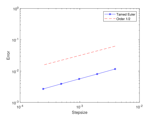
Figure 1. Root mean square approximation error versus time-stepsize.

To clearly display the convergence rate of the tamed Euler scheme at the time $T=1$, we plot our approximation of the root mean-square errors as a function of the stepsize $h=1/n$ in log-log scale in Figure 1, where the expectation is approximated by the mean of $10^{5}$ independent realizations. Since there is no explicit solution available for the SDE (54), we use the tamed Euler scheme with a fine stepsize $h=2^{-16}$ to obtain the reference solution. As predicted, the tamed Euler scheme gives errors that decrease proportional to $h$, indicating that the scheme converges strongly with the standard order $1/2$ to the exact solution of the SDE.

References

- [1] Guo, Q., Liu, W., and Mao, X. A note on the partially truncated Euler–Maruyama method. Appl. Numer. Math. 130 (2018), 157–170.
- [2] Guo, Q., Liu, W., Mao, X., and Yue, R. The partially truncated Euler–Maruyama method and its stability and boundedness. Appl. Numer. Math. 115 (2017), 235–251.
- [3] Guo, Q., Liu, W., Mao, X., and Yue, R. The truncated Milstein method for stochastic differential equations with commutative noise. J. Comput. Appl. Math. 338 (2018), 298–310.
- [4] Hu, L., Li, X., and Mao, X. Convergence rate and stability of the truncated Euler–Maruyama method for stochastic differential equations. J. Comput. Appl. Math. 337 (2018), 274–289.
- [5] Hutzenthaler, M., Jentzen, A., and Kloeden, P. E. Strong and weak divergence in finite time of Euler’s method for stochastic differential equations with non-globally Lipschitz continuous coefficients. Proc. Math. Phys. Eng. Sci. 467 (2011), 1563–1576.
- [6] Hutzenthaler, M., Jentzen, A., and Kloeden, P. E. Strong convergence of an explicit numerical method for SDEs with nonglobally Lipschitz continuous coefficients. Ann. Appl. Probab. 22 (2012), 1611–1641.
- [7] Karatzas, I., and Shreve, S. E. Brownian Motion and Stochastic Calculus, 1st ed., vol. 113 of Graduate Texts in Mathematics. Springer-Verlag, New York, 1988.
- [8] Leobacher, G., and Szölgyenyi, M. A numerical method for SDEs with discontinuous drift. BIT Numer. Math. 56 (2016), 151–162.
- [9] Leobacher, G., and Szölgyenyi, M. Convergence of the Euler–Maruyama method for multidimensional SDEs with discontinuous drift and degenerate diffusion coefficient. Numer. Math. 138 (2018), 219–239.
- [10] Mao, X. Stochastic Differential Equations and Applications, 2nd ed. Horwood Publishing Limited, Chichester, 2007.
- [11] Mao, X. The truncated Euler–Maruyama method for stochastic differential equations. J. Comput. Appl. Math. 290 (2015), 370–384.
- [12] Mao, X. Convergence rates of the truncated Euler–Maruyama method for stochastic differential equations. J. Comput. Appl. Math. 296 (2016), 362–375.
- [13] Müller-Gronbach, T., Sabanis, S., and Yaroslavtseva, L. Existence, uniqueness and approximation of solutions of SDEs with superlinear coefficients in the presence of discontinuities of the drift coefficient. ArXiv: 2204.02343 (2022).
- [14] Müller-Gronbach, T., and Yaroslavtseva, L. On the performance of the Euler–Maruyama scheme for SDEs with discontinuous drift coefficient. Ann. Inst. H. Poincaré Probab. Statist. 56 (2020), 1162–1178.
- [15] Neuenkirch, A., and Szölgyenyi, M. The Euler–Maruyama scheme for SDEs with irregular drift: convergence rates via reduction to a quadrature problem. IMA J. Numer. Anal. 41 (2021), 1164–1196.
- [16] Revuz, D., and Yor, M. Continuous Martingales and Brownian Motion, 3rd ed. Springer-Verlag, Berlin, 1999.
- [17] Sabanis, S. A note on tamed Euler approximations. Electron. Commun. Probab. 18 (2013), 1–10.
- [18] Sabanis, S. Euler approximations with varying coefficients: the case of superlinearly growing diffusion coefficients. Ann. Appl. Probab. 26 (2016), 2083–2105.
- [19] Tretyakov, M. V., and Zhang, Z. A fundamental mean-square convergence theorem for SDEs with locally Lipschitz coefficients and its applications. SIAM J. Numer. Anal. 51 (2013), 3135–3162.
- [20] Wang, X., and Gan, S. The tamed Milstein method for commutative stochastic differential equations with non-globally Lipschitz continuous coefficients. J. Differ. Equ. Appl. 19 (2013), 466–490.
- [21] Zhang, Z., and Ma, H. Order-preserving strong schemes for SDEs with locally Lipschitz coefficients. Appl. Numer. Math. 112 (2017), 1–16.
- [22] Zong, X., Wu, F., and Huang, C. Convergence and stability of the semi-tamed Euler scheme for stochastic differential equations with non-Lipschitz continuous coefficients. Appl. Math. Comput. 228 (2014), 240–250.