New asymptotically flat static vacuum metrics with near Euclidean boundary data

Abstract.

In our prior work toward Bartnik’s static vacuum extension conjecture for near Euclidean boundary data, we establish a sufficient condition, called static regular, and confirm large classes of boundary hypersurfaces are static regular. In this note, we further improve some of those prior results. Specifically, we show that any hypersurface in an open and dense subfamily of a certain general smooth one-sided family of hypersurfaces (not necessarily a foliation) is static regular. The proof uses some of our new arguments motivated from studying the conjecture for boundary data near an arbitrary static vacuum metric.

1. Introduction

Let $n\geq 3$ and $(M,g)$ be an $n$-dimensional Riemannian manifold. We say that $(M,g)$ is static vacuum (or $g$ is a static vacuum metric on $M$) if there is a scalar-valued function $u$ on $M$ satisfying

$$\begin{split}-u\mathrm{Ric}_{g}+\nabla^{2}_{g}u&=0\\ \Delta_{g}u&=0.\end{split}$$ (1.1)

Such $u$ is called a static potential. The class of static vacuum metrics has played a fundamental role in general relativity because when $u>0$, the triple $(M,g,u)$ gives rise to a Ricci flat spacetime $(\mathbb{R}\times M,-u^{2}dt^{2}+g)$ that has a global Killing vector field $\partial_{t}$.

A very important example of asymptotically flat, static vacuum metrics is the the family of (Riemannian) Schwarzschild metrics $g_{m}$:

$$g_{m} =\left(1-\tfrac{2m}{r^{n-2}}\right)^{-1}dr^{2}+r^{2}g_{S^{n-1}}\quad\mbox{ defined on }\mathbb{R}^{n}\setminus B_{(2m)^{\frac{1}{n-2}}},$$

with the static potential $u_{m}=\sqrt{1-\tfrac{2m}{r^{n-2}}}$, where $g_{S^{n-1}}$ is the standard metric on the unit sphere $S^{n-1}$. Note that the Schwarzschild metrics are rotationally symmetric. When $m=0$, the Schwarzschild metric becomes the Euclidean metric. When $m>0$, the Schwarzschild manifold has a minimal hypersurface boundary, precisely at $u=0$. In fact, the Schwarzschild metrics are the only asymptotically flat, static vacuum 3-manifolds with such property, by the celebrated Uniqueness Theorem of Static Black Holes. See [13, 18, 9]. Another family of static vacuum, exact solutions was discovered by H. Weyl. The Weyl solutions are axially symmetric and have general asymptotics at infinity, but a subclass of them can have asymptotically flat end. Those exact solutions can be characterized by certain conditions (e.g. having black hole boundary), and great efforts have been made toward the uniqueness and classification results of those static vacuum metrics. See, for example, M. Reiris and J. Peraza [17] and the references therein.

In contrast, Robert Bartnik conjectured the following “prescribing boundary value” problem for asymptotically flat, static vacuum manifolds [8, Conjecture 7]. The conjecture was originated from his quasi-local mass program in 1989, for which we refer the reader to the survey article of M. Anderson [5] for details. The conjecture itself is also of independent interest as a natural geometric PDE boundary value problem. Furthermore, progress toward this conjecture would give rise to new examples of asymptotically flat, static vacuum metrics and advance our understanding toward the structure of static vacuum metrics.

Conjecture 1 (Static Extension Conjecture).

Let $(\Omega,g_{0})$ be a compact manifold with scalar curvature $R_{g_{0}}\geq 0$. Suppose the mean curvature $H_{g_{0}}$ is positive somewhere on the boundary $\Sigma$. Then there exists a unique asymptotically flat, static vacuum manifold $(M,g)$ with boundary $\partial M\cong\Sigma$ satisfying

$$\begin{array}[]{ll}g_{0}^{\intercal}=g^{\intercal}\\ H_{g_{0}}=H_{g}\end{array}\quad\mbox{ on }\Sigma.$$

Here, $(\cdot)^{\intercal}$ denotes the restriction on the tangent bundle of $\Sigma$.

Convention: The mean curvature $H_{g}$ of a hypersurface $\Sigma$ in a Riemannian manifold $(M,g)$ is defined as $H_{g}=\operatorname{div}_{g}\nu$, where $\nu$ is the unit normal vector of $\Sigma$. When $(M,g)$ is asymptotically flat, we choose $\nu$ to point to infinity (and thus the unit normal for $\Sigma$ in $(\Omega,g_{0})$ points outward).

We shall refer to the geometric boundary data $(g_{0}^{\intercal},H_{g_{0}})$ as the Bartnik boundary data. Let us also remark on the assumption that $H_{g_{0}}$ is positive somewhere. The conjecture would fail without this assumption because such extension, if exist, would contain a minimal hypersurface homologous to the boundary (at least in dimensions $n\leq 7$), and the extension must be Schwarzschild by Uniqueness Theorem, which put strong restriction on $g_{0}^{\intercal}$. See P. Miao [15] for $n=3$. For $n\leq 7$, by minimal surface theory, there is an outermost minimal hypersurface homologous to the boundary. By the result of D. Martin, Miao, and the second author [12, Theorem 1], the static potential $u=0$ on the outmost minimal hypersurface. From there, one applies the generalization of Uniqueness of Static Black holes in higher dimensions by G. Gibbons, D. Ida, and T. Shiromizu [11].

Even with the mean curvature assumption, it is highly speculated that Conjecture 1 does not hold in general as stated. Let $\Omega$ be a bounded open subset in $\mathbb{R}^{n}$. Observed by [7, 6], if the boundary $\Sigma=\partial\overline{\Omega}$ is only inner embedded, i.e., $\Sigma$ touches itself from the exterior region $\mathbb{R}^{n}\setminus\Omega$, the induced data $(\bar{g}^{\intercal},H_{\bar{g}})$ is valid Bartnik boundary data, but $(\bar{g},1)$ in $\mathbb{R}^{n}\setminus\Omega$ is not a valid static vacuum extension as $\mathbb{R}^{n}\setminus\Omega$ is not a manifold with boundary. One can further arrange so that the mean curvature $H_{\bar{g}}$ is positive everywhere. Those inner embedded hypersurfaces are conjectured to be counter-examples to Conjecture 1 by [6, Conjecture 5.2] (see also [5]), though it is not clear whether there could be another static vacuum extension far way from $(\mathbb{R}^{n}\setminus\Omega,\bar{g},1)$. Nevertheless, positive results to Conjecture 1, under suitable assumptions, will provide a structure theory for the space of static vacuum metrics (parametrized by their Bartnik boundary data). It also connects the fundamental problem on isometric embeddings of hypersurfaces into a static vacuum manifold with prescribed mean curvature. In particular, that question apparently has intriguing connections to the work of P.-N. Chen, M.-T. Wang, Y.-K. Wang, and S.-T. Yau  [10] where the notion of quasi-local energy defined via isometric embeddings into a reference static metric is proposed, extending the celebrated Wang-Yau quasi-local mass with respect to the Minkowski spacetime [19].

There are some positive results toward Conjecture 1. The existence and local uniqueness is proven for $n=3$ and for $(g_{0},H_{g_{0}})$ sufficiently close to the induced Bartnik boundary data on a round sphere from the Euclidean metric, i.e. $(g_{0},H_{g_{0}})$ sufficiently close to $(g_{S^{2}},2)$. See Miao [14], Anderson-Khuri [7], and Anderson  [4]. In recent work [1], we give a general framework to tackle Conjecture 1 and confirm existence and local uniqueness of Conjecture 1 for large classes of boundary data, including those close to the induced boundary data on either any star-shaped hypersurfaces or quite general perturbed hypersurfaces in the Euclidean space. In this present note, we improve Theorem 7 in [1], by employing new arguments in our recent work [2]. The new results are presented as Theorem 7, Corollary 8, and Theorem 9 below.

To describe the new results, we first recall the basic notations and definitions and review relevant results from [1].

Let $\Omega$ be a bounded open subset in $\mathbb{R}^{n}$ whose boundary $\Sigma=\partial\overline{\Omega}$ is a connected, embedded smooth hypersurface in $\mathbb{R}^{n}$. We denote by $\bar{g}$ the Euclidean metric in $\mathbb{R}^{n}$ with $\bar{g}_{ij}=\delta_{ij}$ (with respect to a fixed Cartesian coordinate chart). Our analytic framework is based on the weighted Hölder spaces $\operatorname{\mathcal{C}}^{k,\alpha}_{-q}(\mathbb{R}^{n}\setminus\Omega)$ (see its definition in Section 2.1 of [1]), and we always assume the Hölder exponent $\alpha\in(0,1)$ and the fall-off rate $q\in(\frac{n-2}{2},n-2)$ for asymptotical flatness. We denote by $D\mathrm{Ric}|_{\bar{g}}(h)$ the linearization of the Ricci curvature at $\bar{g}$; namely, let $g(t)$ be an arbitrary family of Riemannian metrics on $\mathbb{R}^{n}\setminus\Omega$ so that $g(0)=\bar{g}$ and $g^{\prime}(0)=h$, then $D\mathrm{Ric}|_{\bar{g}}(h):=\left.\frac{d}{dt}\right|_{t=0}\mathrm{Ric}_{g(t)}$. Similarly, we define the linearizations of the mean curvature and second fundamental form on $\Sigma$ by $DH|_{\bar{g}}(h)$ and $DA|_{\bar{g}}(h)$, respectively. We will omit the subscript $\bar{g}$ in those linearizations when the context is clear.

Definition 2.

The boundary $\Sigma$ is said to be static regular in $\mathbb{R}^{n}\setminus\Omega$ if for any pair of a symmetric $(0,2)$-tensor $h$ and a scalar-valued function $v$ satisfying $(h,v)\in\operatorname{\mathcal{C}}^{2,\alpha}_{-q}(\mathbb{R}^{n}\setminus\Omega)$ and

$$\begin{split}-D\mathrm{Ric}(h)+\nabla^{2}v&=0,\quad\Delta v=0\quad\mbox{ in }\mathbb{R}^{n}\setminus\Omega,\\ h^{\intercal}&=0,\quad DH(h)=0\quad\mbox{ on }\Sigma,\end{split}$$ (1.2)

we must have $DA(h)=0$ on $\Sigma$.

The following fundamental result obtained in [1] says that “static regular” is a sufficient condition for existence and local uniqueness.

Theorem 3 ([1, Theorem 3]).

Suppose the boundary $\Sigma$ is static regular in $\mathbb{R}^{n}\setminus\Omega$. Then there exist positive constants $\epsilon_{0},C$ such that for each $\epsilon\in(0,\epsilon_{0})$, if $(\tau,\phi)$ satisfies $\|(\tau,\phi)-(\bar{g}^{\intercal},H_{\bar{g}})\|_{\operatorname{\mathcal{C}}^{2,\alpha}(\Sigma)\times\operatorname{\mathcal{C}}^{1,\alpha}(\Sigma)}<\epsilon$, then there exists an asymptotically flat pair $(g,u)$ with $\|(g,u)-(\bar{g},1)\|_{\operatorname{\mathcal{C}}^{2,\alpha}_{-q}(\mathbb{R}^{n}\setminus\Omega)}<C\epsilon$ such that $(g,u)$ is a static vacuum pair in $\mathbb{R}^{n}\setminus\Omega$ having the Bartnik boundary data $(g^{\intercal},H_{g})=(\tau,\phi)$ on $\Sigma$.

Furthermore, the solution $(g,u)$ is geometrically unique in a neighborhood $\mathcal{U}$ of $(\bar{g},1)$ in the $\operatorname{\mathcal{C}}^{2,\alpha}_{-q}(\mathbb{R}^{n}\setminus\Omega)$-norm.

We remark that the “local uniqueness” in the above theorem is precisely described under the static-harmonic gauge and the orthogonal gauge. Since we will not explicitly use them in the present paper, we refer the reader to the discussion right after Theorem 3 in [1].

In [1], we furthermore show that large classes of hypersurfaces in $\mathbb{R}^{n}$ are static regular. In particular, we show that static regular hypersurfaces are “dense” in the following concrete sense. A family of embedded hypersurfaces $\{\Sigma_{t}\}\subset\mathbb{R}^{n}$ is said to form a smooth generalized foliation if the deformation vector $X$ of $\{\Sigma_{t}\}$ is smooth and on each $\Sigma_{t}$, $\bar{g}(X,\nu)=\zeta$ where $\zeta>0$ in a dense subset of $\Sigma_{t}$, and $\nu$ is the unit normal of $\Sigma_{t}$. In other words, $\{\Sigma_{t}\}$ is slightly more general than a foliation in that the leaves can overlap on a nowhere dense subset.

Theorem 4 ([1, Theorem 7]).

Let $\delta>0$, $t\in[-\delta,\delta]$, and each $\Omega_{t}\subset\mathbb{R}^{n}$ be a bounded open subset with hypersurface boundary $\Sigma_{t}=\partial\overline{\Omega_{t}}$ embedded in $\mathbb{R}^{n}$. Suppose the boundaries $\{\Sigma_{t}\}$ form a smooth generalized foliation. Then there is an open dense subset $J\subset(-\delta,\delta)$ such that $\Sigma_{t}$ is static regular in $\mathbb{R}^{n}\setminus\Omega_{t}$ for all $t\in J$.

The above theorem has the following strong consequence because of the dilation property of the Euclidean static vacuum pair.

Corollary 5 ([1, Corollary 8]).

Let $\Omega$ be a bounded open subset in $\mathbb{R}^{n}$ whose boundary $\Sigma=\partial\overline{\Omega}$ is a star-shaped hypersurface. Then $\Sigma$ is static regular in $\mathbb{R}^{n}\setminus\Omega$.

The purpose of this note is to extend Theorem 4.

Definition 6.

A collection of embedded hypersurfaces $\{\Sigma_{t}\}\subset\mathbb{R}^{n}$ is a smooth one-sided family of hypersurfaces foliating along $\hat{\Sigma}_{t}\subset\Sigma_{t}$ with relatively simply-connected $\Sigma_{t}\setminus\hat{\Sigma}_{t}$ if the deformation vector $X$ of $\{\Sigma_{t}\}$ is smooth and on each $\Sigma_{t}$, $\bar{g}(X,\nu)=\zeta\geq 0$ with $\zeta>0$ in a dense subset of each $\hat{\Sigma}_{t}\subset\Sigma_{t}$ satisfying $\pi_{1}(\Sigma_{t},\hat{\Sigma}_{t})=0$.

For a subset $U$ in $M$, the condition $\pi_{1}(M,U)=0$ says that $U$ is connected and the inclusion map $U\hookrightarrow M$ induces a surjection $\pi_{1}(U)\rightarrow\pi_{1}(M)$. In our setting, we clearly have $\pi_{1}(\mathbb{R}^{n}\setminus\Omega,\Sigma)=0$. Thus, the additional condition for a subset $\hat{\Sigma}\subset\Sigma$ to satisfy $\pi_{1}(\Sigma,\hat{\Sigma})=0$ implies $\pi_{1}(\mathbb{R}^{n}\setminus\Omega,\hat{\Sigma})=0$. In loose terms, the later condition implies that for any point $x\in\mathbb{R}^{n}\setminus\Omega$, all paths from $x$ to $\hat{\Sigma}$ are (homotopically) equivalent. See Figure 1 below. This property is used in Theorem 2.5 below to ensure certain global extensions of local vector fields.

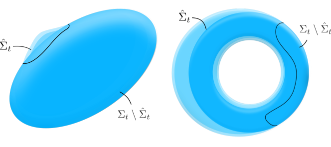
Figure 1. Each figure illustrates Definition 6 that $\{\Sigma_{t}\}$ foliates along $\hat{\Sigma}_{t}$ with relatively simply-connected $\Sigma_{t}\setminus{\hat{\Sigma}}_{t}$. In the left figure, a one-sided family of (topological) spheres $\{\Sigma_{t}\}$ is shown where $\hat{\Sigma}_{t}$ can be very small. In other words, $\Sigma_{t}$ can largely overlap on $\Sigma_{t}\setminus\hat{\Sigma}_{t}$. The right figure illustrates a one-sided family of (topological) tori with $\pi_{1}(\Sigma_{t},\hat{\Sigma}_{t})=0$.

Note that a smooth generalized foliation $\{\Sigma_{t}\}$ defined earlier is necessarily a smooth one-sided family of hypersurfaces foliating along $\hat{\Sigma}_{t}\subset\Sigma_{t}$ with relatively simply-connected $\Sigma_{t}\setminus\hat{\Sigma}_{t}$ (by letting $\hat{\Sigma}_{t}=\Sigma_{t}$). However, a smooth one-sided family $\{\Sigma_{t}\}$ in the above sense may not form a foliation because the leaves can overlap on $\Sigma_{t}\setminus\hat{\Sigma}_{t}$. The following theorem generalizes Theorem 4.

Theorem 7.

Let $\delta>0$, $t\in[-\delta,\delta]$, and each $\Omega_{t}\subset\mathbb{R}^{n}$ be a bounded open subset with hypersurface boundary $\Sigma_{t}=\partial\overline{\Omega_{t}}$ embedded in $\mathbb{R}^{n}$. Suppose the boundaries $\{\Sigma_{t}\}$ form a smooth one-sided family of hypersurfaces foliating along $\hat{\Sigma}_{t}\subset\Sigma_{t}$ with relatively simply-connected $\Sigma_{t}\setminus\hat{\Sigma}_{t}$. Then there is an open dense subset $J\subset(-\delta,\delta)$ such that $\Sigma_{t}$ is static regular in $\mathbb{R}^{n}\setminus\Omega_{t}$ for all $t\in J$.

In the special case that $\Sigma$ is simply-connected (e.g., $\Sigma$ is a topological sphere), we trivially have $\pi_{1}(\Sigma,\hat{\Sigma})=0$ for any nonempty connected subset $\hat{\Sigma}$. Slight perturbation on $\hat{\Sigma}$ produces a one-sided family $\{\Sigma_{t}\}$ with $\Sigma_{0}=\Sigma$ that foliates along small subsets ${\hat{\Sigma}}_{t}\subset\Sigma_{t}$ so that $\Sigma_{t}\setminus\hat{\Sigma}_{t}$ coincides with $\Sigma\setminus\hat{\Sigma}$ for all $t$. See the left figure in Figure 1. Theorem 7 says that $\Sigma_{t}$ is static regular for $t$ in an open and dense set. Together with Theorem 3, we give the following corollary that one can solve for static vacuum extensions whose boundary data are arbitrarily close to the induced boundary data $(\bar{g}^{\intercal},H_{\bar{g}})$ on $\Sigma$, except a small subset $\hat{\Sigma}\subset\Sigma$.

Corollary 8.

Let $\Sigma=\partial\overline{\Omega}$ be a simply-connected, closed, embedded hypersurface in $\mathbb{R}^{n}$. Given any nonempty open subset $\hat{\Sigma}\subset\Sigma$ and any $\delta>0$, there exists $(\tau_{0},\phi_{0})\in\operatorname{\mathcal{C}}^{2,\alpha}(\Sigma)\times\operatorname{\mathcal{C}}^{1,\alpha}(\Sigma)$ and constants $\epsilon_{0},C>0$ satisfying

$$(\tau_{0},\phi_{0})=(\bar{g}^{\intercal},H_{\bar{g}})\mbox{ on }\Sigma\setminus\hat{\Sigma}$$

$$\|(\tau_{0},\phi_{0})-(\bar{g}^{\intercal},H_{\bar{g}})\|_{\operatorname{\mathcal{C}}^{2,\alpha}(\hat{\Sigma})\times\operatorname{\mathcal{C}}^{1,\alpha}(\hat{\Sigma})}<\delta$$

such that for each $\epsilon\in(0,\epsilon_{0})$, if $(\tau,\phi)$ satisfies $\|(\tau,\phi)-(\tau_{0},\phi_{0})\|_{\operatorname{\mathcal{C}}^{2,\alpha}(\Sigma)\times\operatorname{\mathcal{C}}^{1,\alpha}(\Sigma)}<\epsilon$, then there exists an asymptotically flat pair $(g,u)$ with $\|(g,u)-(\bar{g},1)\|_{\operatorname{\mathcal{C}}^{2,\alpha}_{-q}(\mathbb{R}^{n}\setminus\Omega)}<C\epsilon$ such that $(g,u)$ is a static vacuum pair in $\mathbb{R}^{n}\setminus\Omega$ having the Bartnik boundary data $(g^{\intercal},H_{g})=(\tau,\phi)$ on $\Sigma$.

Furthermore, the solution $(g,u)$ is geometrically unique in a neighborhood $\mathcal{U}$ of $(\bar{g},1)$ in the $\operatorname{\mathcal{C}}^{2,\alpha}_{-q}(\mathbb{R}^{n}\setminus\Omega)$-norm.

The proof to Theorem 7 involves several new arguments used in our recent work for general asymptotically flat, static vacuum background metrics [2]. One of the key arguments is the following theorem, which can be viewed as a uniqueness theorem for “localized” boundary data.

Theorem 9.

Let $\hat{\Sigma}$ be an open subset of $\Sigma$ (can be the entire $\Sigma$) satisfying $\pi_{1}(\Sigma,\hat{\Sigma})=0$. Let $(h,v)\in\operatorname{\mathcal{C}}^{2,\alpha}_{-q}(\mathbb{R}^{n}\setminus\Omega)$ solve

$$\left\{\begin{array}[]{l}-D\mathrm{Ric}(h)+\nabla^{2}v=0\\ \Delta v=0\end{array}\right.\mbox{ in }\mathbb{R}^{n}\setminus\Omega$$

$$\left\{\begin{array}[]{l}h^{\intercal}=0\\ DA(h)=0\\ D(\nabla_{\nu}A)(h)=0\end{array}\right.\quad\mbox{ on }\hat{\Sigma}$$

where $D(\nabla_{\nu}A)(h)$ denotes the linearization of $\nabla_{\nu}A$. Then there is a vector field $X\in\operatorname{\mathcal{C}}^{3,\alpha}_{\mathrm{loc}}(\mathbb{R}^{n}\setminus\Omega)$ satisfying $X=0$ on $\hat{\Sigma}$ and $X-K\in\operatorname{\mathcal{C}}^{3,\alpha}_{-q}(\mathbb{R}^{n}\setminus\Omega)$ for some Euclidean Killing vector field $K$ (possibly zero) such that

$$h=L_{X}\bar{g}\quad\mbox{ and }\quad v=0\quad\mbox{ in }\mathbb{R}^{n}\setminus\Omega.$$

Furthermore, if $h^{\intercal}=0$ and $DH(h)=0$ everywhere on $\Sigma$, then $X=0$ everywhere on $\Sigma$ and thus $DA(h)=0$ on $\Sigma$.

Theorem 9 says that the solutions must be “trivial” in the sense that $(h,v)$ must arise from “infinitesimal” diffeomorphisms. More precisely, if we let $X$ be a vector field as in the above theorem and let $\phi_{t}$ be the family of diffeomorphisms on $\mathbb{R}^{n}\setminus\Omega$ generated from $X$ (in particular, $\phi_{t}$ is the identity map on $\Sigma$ for all $t$). Then the family of static vacuum pairs $(g_{t},u_{t})=\phi_{t}^{*}(\bar{g},1)$ as the pull-back pairs of $(\bar{g},1)$ would also satisfy (1.1) and have the same boundary data $(\bar{g}^{\intercal},A_{\bar{g}},\nabla_{\nu}A_{\bar{g}})$ on $\hat{\Sigma}$ (in fact on the entire $\Sigma$). The linearization of $(g_{t},u_{t})$ becomes $(L_{X}\bar{g},X(1))=(L_{X}\bar{g},0)$, which satisfies the linearized system in Theorem 9. On the other hand, Theorem 9 says that those are the only solutions.

The rest of this note is organized as follows: Theorem 9 is proved in Section 2, and then Theorem 7 is proved in Section 3.

2. Localized boundary data

The major motivation for the definition of static regular, Definition 2, is the following uniqueness theorem for Cauchy boundary data from [1].

Theorem 2.1.

Let $(h,v)\in\operatorname{\mathcal{C}}^{2,\alpha}_{-q}(\mathbb{R}^{n}\setminus\Omega)$ solve

$$\left\{\begin{array}[]{l}-D\mathrm{Ric}(h)+\nabla^{2}v=0\\ \Delta v=0\end{array}\right.\mbox{ in }\mathbb{R}^{n}\setminus\Omega$$

$$\left\{\begin{array}[]{l}h^{\intercal}=0\\ DA(h)=0\end{array}\right.\quad\mbox{ on }\Sigma.$$

Then there is a vector field $X\in\operatorname{\mathcal{C}}^{3,\alpha}_{\mathrm{loc}}(\mathbb{R}^{n}\setminus\Omega)$ satisfying $X=0$ on $\Sigma$ and $X-K\in\operatorname{\mathcal{C}}^{3,\alpha}_{1-q}(\mathbb{R}^{n}\setminus\Omega)$ for some Euclidean Killing vector field $K$ (possibly zero) such that

$$h=L_{X}\bar{g}\quad\mbox{ and }\quad v=0\mbox{ in }\mathbb{R}^{n}\setminus\Omega.$$

Proof.

From the proof of Lemma 4.8 in [1], we see that $v=0$ in $\mathbb{R}^{n}\setminus\Omega$. Therefore, $h$ is a Ricci flat deformation in the sense that $D\mathrm{Ric}(h)=0$ in $\mathbb{R}^{n}\setminus\Omega$. Then by Theorem 2.8 of [1], we get the desired conclusion. ∎

The goal of this section is to prove Theorem 9, whose main difference from the above theorem is that the boundary conditions for Theorem 9 are “localized” only on a subset $\hat{\Sigma}\subset\Sigma$ satisfying $\pi_{1}(\Sigma,\hat{\Sigma})=0$.

We will first establish some basic results, and then Theorem 9 follows immediately after proving Proposition 2.4 and Proposition 2.6 below.

We say that a symmetric $(0,2)$-tensor $h$ is said to satisfy the geodesic gauge (of order $2$) on $\Sigma$ if

$$h(\nu,\cdot)=0,\quad(\nabla_{\nu}h)(\nu,\cdot)=0,\quad(\nabla_{\nu}^{2}h)(\nu,\cdot)=0\quad\mbox{ on }\Sigma$$

where $\nu$ is the unit normal vector of $\Sigma$ parallelly extended into a collar neighborhood of $\Sigma$.

Following the same argument as in [1, Lemma 2.5], we see that any tensor $h$ can be “transformed” to satisfy the geodesic gauge.

Lemma 2.2 (Cf. [1, Lemma 2.5]).

Let $h\in\operatorname{\mathcal{C}}^{2,\alpha}_{\mathrm{loc}}(\mathbb{R}\setminus\Omega)$ be a symmetric $(0,2)$-tensor. Then there exists a vector field $V\in\operatorname{\mathcal{C}}^{3,\alpha}$ with $V=0$ on $\Sigma$ and $V$ vanishing outside a collar neighborhood of $\Sigma$ such that $k:=h+L_{V}\bar{g}$ satisfies the geodesic gauge on $\Sigma$.

The following lemma gives an analytic interpretation for the geometric boundary conditions of Theorem 9.

Lemma 2.3.

Let $\hat{\Sigma}$ be an open subset of the boundary $\Sigma$ (can be the entire $\Sigma$). Suppose $h\in\operatorname{\mathcal{C}}^{2,\alpha}_{\mathrm{loc}}(\mathbb{R}^{n}\setminus\Omega)$ satisfies the geodesic gauge and

$$h^{\intercal}=0,\quad DA(h)=0,\quad D(\nabla_{\nu}A)(h)=0\quad\mbox{ on }\hat{\Sigma}.$$

Then

$$h=0,\quad\nabla h=0,\quad\nabla^{2}h=0\quad\mbox{ on }\hat{\Sigma}.$$

Proof.

The first identity is an immediate consequence of $h^{\intercal}=0$ and the geodesic gauge.

To show the second identity, it suffices to show $(\nabla_{\nu}h)^{\intercal}=0$ because $(\nabla_{\mathrm{arbitrary}}h)(\nu,\cdot)=0$ and $(\nabla_{\mathrm{tangential}}h)^{\intercal}=0$ from $h=0$ and geodesic gauge. Recall the formula (see [1, Equation (2.3)])

$$DA(h) =\tfrac{1}{2}(\nabla_{\nu}h)^{\intercal}+A\circ h-\tfrac{1}{2}L_{\omega}g^{\intercal}-\tfrac{1}{2}h(\nu,\nu)A$$ (2.1)

where the one-form $\omega$ is defined by $\omega(\cdot)=h(\nu,\cdot)$, $A$ is the second fundamental form of $\Sigma\subset(\mathbb{R}^{n},\bar{g})$, and $(A\circ h)_{ab}=\tfrac{1}{2}(A_{ac}h_{b}^{c}+A_{bc}h^{c}_{a})$. Therefore, the assumption $DA(h)=0$ implies that $(\nabla_{\nu}h)^{\intercal}=0$ and thus $\nabla h=0$.

To show $\nabla^{2}h=0$, we just need to show that $(\nabla_{\nu}^{2}h)^{\intercal}=0$ because $\nabla_{\mathrm{tangential}}(\nabla h)=0$ and $\nabla_{\nu}\nabla_{\mathrm{tangential}}h=\nabla_{\mathrm{tangential}}\nabla_{\nu}h$ plus terms involving $h$ and $\nabla h$, which are all zero on $\hat{\Sigma}$. Note that since $h$ satisfies the geodesic gauge, we also have $\nabla_{\nu}(DA)(h)=D(\nabla_{\nu}A)(h)$ on $\hat{\Sigma}$. To see this, we compute, for tangential vectors $e_{a},e_{b}$ to $\Sigma$:

$$\begin{split}\Big{(}D(\nabla_{\nu}A)(h)\Big{)}(e_{a},e_{b})&:=\left.\frac{d}{dt}\right|_{t=0}\big{(}\nabla_{\nu_{g(t)}}A_{g(t)}\big{)}(e_{a},e_{b})\\ &=\Big{(}\nabla_{\nu}(DA)(h)\Big{)}(e_{a},e_{b})+\big{(}(\nabla_{\nu_{g(t)}})^{\prime}A\big{)}(e_{a},e_{b})\\ &=\Big{(}\nabla_{\nu}(DA)(h)\Big{)}(e_{a},e_{b})\end{split}$$ (2.2)

where in the the second line $(\nabla_{\nu_{g(t)}})^{\prime}:=\left.\frac{d}{dt}\right|_{t=0}\nabla_{\nu_{g(t)}}$ and one can verify that $\big{(}(\nabla_{\nu_{g(t)}})^{\prime}A\big{)}(e_{a},e_{b})$ because $h=0$ and $\nabla h=0$ on $\hat{\Sigma}$.

To conclude, we get $\nabla_{\nu}(DA)(h)=0$ on $\hat{\Sigma}$ using (2.2) and the assumption that $D\big{(}\nabla_{\nu}A\big{)}(h)=0$ on $\hat{\Sigma}$. Covariant differentiating (2.1) in $\nu$, we obtain $(\nabla_{\nu}^{2}h)^{\intercal}=0$.

∎

Proposition 2.4.

Let $\hat{\Sigma}$ be an open subset of $\Sigma$ (can be the entire $\Sigma$). Let $(h,v)\in\operatorname{\mathcal{C}}^{2,\alpha}_{-q}(\mathbb{R}^{n}\setminus\Omega)$ solve

$$\left\{\begin{array}[]{l}-D\mathrm{Ric}(h)+\nabla^{2}v=0\\ \Delta v=0\end{array}\right.\mbox{ in }\mathbb{R}^{n}\setminus\Omega$$

$$\left\{\begin{array}[]{l}h^{\intercal}=0\\ DA(h)=0\\ D\big{(}\nabla_{\nu}A\big{)}(h)=0\end{array}\right.\quad\mbox{ on }\hat{\Sigma}.$$

Then $v\equiv 0$ and $D\mathrm{Ric}(h)=0$ in $\mathbb{R}^{n}\setminus\Omega$.

Proof.

By Lemma 2.2, we may assume $h$ satisfies the geodesic gauge. The boundary conditions and Lemma 2.3 imply that $h=0,\nabla h=0,\nabla^{2}h=0$ on $\hat{\Sigma}$.

Note that $D\mathrm{Ric}(h)$ involves $h$ and its derivatives up to the second order; precisely, in local coordinates (see, e.g. [1, Equation (2.1)]):

$$(D\mathrm{Ric}|_{g}(h))_{ij} =-\tfrac{1}{2}g^{k\ell}h_{ij;k\ell}+\tfrac{1}{2}g^{k\ell}(h_{ik;\ell j}+h_{jk;\ell i})-\tfrac{1}{2}(\operatorname{tr}h)_{ij}$$

$$\quad+\tfrac{1}{2}(R_{i\ell}h^{\ell}_{j}+R_{j\ell}h^{\ell}_{i})-R_{ik\ell j}h^{k\ell}\quad\mbox{ for all }i,j=0,1,\dots,n-1.$$

Restricting $-D\mathrm{Ric}(h)+\nabla^{2}v=0$ on the boundary, we see $\nabla^{2}v=0$ on $\hat{\Sigma}$.

Next, we define the function $f=\frac{\partial v}{\partial x_{i}}$ for some $i=1,\dots,n$, where $(x_{1},\dots,x_{n})$ are the Cartesian coordinates. Since $v$ is harmonic, $f$ is also a harmonic function in $\mathbb{R}^{n}\setminus\Omega$. The conditions that $\nabla^{2}v=0$ on $\hat{\Sigma}$ imply

$$\nabla^{\Sigma}f=0\quad\mbox{ and }\quad\nu(f)=0\qquad\mbox{ on }\hat{\Sigma}.$$

The first identity implies $f\equiv c$ for some constant $c$ in a connected open subset of $\hat{\Sigma}$. Together with the second identity and uniqueness of Cauchy boundary value for the harmonic equation, we conclude that $f\equiv c$ everywhere in $\mathbb{R}^{n}\setminus\Omega$. Since $f\rightarrow 0$ by the fall-off rate of $v$, we see that $f=\frac{\partial v}{\partial x_{i}}$ is identically zero. Since $i$ is arbitrary, we see that $\nabla v=0$ and thus $v$ is constant. Since $v\rightarrow 0$ at infinity, we conclude that $v$ is identically zero. ∎

In the above proposition, we have shown $D\mathrm{Ric}(h)=0$ in $\mathbb{R}^{n}\setminus\Omega$. Proposition 2.6 below generalizes Theorem 2.8 of [1], where $\hat{\Sigma}$ was assumed to be the entire boundary $\Sigma$. The key argument is the following extension theorem for $h$-Killing vector fields, that extends the classical result of Nomizu for the case $h$ is identically zero [16].

Theorem 2.5 ([2, Theorem 7], Cf. [3, Lemma 2.6]).

Let $(M,g)$ be a connected, analytic Riemannian manifold. Let $h$ be an analytic, symmetric $(0,2)$-tensor on $M$. Let $U\subset M$ be a connected open subset satisfying $\pi_{1}(M,U)=0$. Then if $h=L_{X}g$ in $U$, there is a unique global vector field $Y$ such that $Y=X$ in $U$ and $h=L_{Y}g$ in the whole manifold $M$.

Proposition 2.6.

Let $\hat{\Sigma}$ be an open subset of $\Sigma$ satisfying $\pi_{1}(\Sigma,\hat{\Sigma})=0$. Let $h\in\operatorname{\mathcal{C}}^{2,\alpha}_{-q}(\mathbb{R}^{n}\setminus\Omega)$ satisfy

$$D\mathrm{Ric}(h)=0\quad\mbox{ in }\mathbb{R}^{n}\setminus\Omega$$

$$\left\{\begin{array}[]{l}h^{\intercal}=0\\ DA(h)=0\end{array}\right.\quad\mbox{ on }\hat{\Sigma}.$$

Then there is a vector field $X\in\operatorname{\mathcal{C}}^{3,\alpha}_{\mathrm{loc}}(\mathbb{R}^{n}\setminus\Omega)$ satisfying $X=0$ on $\hat{\Sigma}$ and $X-K\in\operatorname{\mathcal{C}}^{3,\alpha}_{-q}(\mathbb{R}^{n}\setminus\Omega)$ for some Euclidean Killing vector field $K$ (possibly zero) such that

$$h=L_{X}\bar{g}\mbox{ in }\mathbb{R}^{n}\setminus\Omega.$$

Furthermore, if $h^{\intercal}=0$ and $DH(h)=0$ everywhere on $\Sigma$, then $X=0$ everywhere on $\Sigma$ and thus $DA(h)=0$ on $\Sigma$.

Proof.

We may without loss of generality assume that $h$ satisfies the geodesic gauge on $\Sigma$. We extend $h$ by $0$ across $\hat{\Sigma}$ into some small open subset $U\subset\Omega$ so that the “extended” manifold $\hat{M}=(\mathbb{R}^{n}\setminus\Omega)\cup\overline{U}$ has smooth embedded boundary $\partial\hat{M}$ and $\pi_{1}(\hat{M},U)=0$. Denote the extension of $h$ by $k\in\operatorname{\mathcal{C}}^{1}_{\mathrm{loc}}(\hat{M})$:

$$k=\left\{\begin{array}[]{ll}h&\mbox{ in }\mathbb{R}^{n}\setminus\Omega\\ 0&\mbox{ in }U\end{array}\right.$$

Let $Z\in\operatorname{\mathcal{C}}^{1,\alpha}_{1-q}(\hat{M})$ be a vector field that weakly solves $\Delta Z=\beta k$ in $\hat{M}$ with $Z=0$ on $\partial\hat{M}$ where the Bianchi operator $\beta k=-\operatorname{div}_{\bar{g}}k+\frac{1}{2}d(\mathrm{tr}_{\bar{g}}k)$. Or equivalently, $k+L_{Z}\bar{g}$ weakly solves $\beta(k+L_{Z}\bar{g})=0$ in $\hat{M}$. Together with the assumption that $D\mathrm{Ric}(h)=0$ in $\mathbb{R}^{n}\setminus\Omega$ and the boundary condition $h=0,\nabla h=0$ on $\Sigma$, we have that $k+L_{Z}\bar{g}$ is a weak solution to $\Delta(k+L_{Z}\bar{g})=0$ in $\hat{M}$. So far, the argument has followed closely [1, Theorem 2.8], to which we refer the analytic details.

But in the current setting we cannot conclude $k+L_{Z}\bar{g}$ is identically zero as in [1, Theorem 2.8]. (In [1], it was possible to extend the harmonic $k+L_{X}\bar{g}$ globally on the entire $\mathbb{R}^{n}$.) Here we apply Weyl’s lemma to see that $k+L_{Z}\bar{g}$ is analytic in $\operatorname{Int}(\hat{M})$. Since $k+L_{Z}\bar{g}=L_{Z}\bar{g}$ in $U$ (remember $k\equiv 0$ there), by Theorem 2.5, there is a unique vector field $Y$ such that $Y=Z$ in $U$ and

$$k+L_{Z}\bar{g}=L_{Y}\bar{g}\mbox{ in }\hat{M}.$$

To summarize, we obtain $X=Y-Z$ with $X=0$ on $\hat{\Sigma}$ and

$$h=L_{X}\bar{g}\quad\mbox{ in }\mathbb{R}^{n}\setminus\Omega.$$

Note that $X\in\operatorname{\mathcal{C}}^{3,\alpha}_{\mathrm{loc}}(\mathbb{R}\setminus\Omega)$ because of the regularity $h$.

The rest of the conclusions follow from basic arguments as in [2], so we just give a sketch below. To show the desired asymptotic of $X$ toward infinity, one first considers the ODE for $X$ along any ray to infinity to show that $X=o(|x|^{2})$. Then writing the equation $D\mathrm{Ric}(L_{X}\bar{g})=0$ in the harmonic gauge gives a harmonic expansion for $X$. Thus $X$ is asymptotic to a Euclidean Killing vector field $K$, using the fall-off rate $L_{X}\bar{g}=h\in\operatorname{\mathcal{C}}^{2,\alpha}_{-q}$.

Lastly, to show that $X=0$ on $\Sigma$ under the added assumptions $h^{\intercal}=0$ and $DH(h)=0$ on $\Sigma$, we write $X=\eta\nu+X^{\intercal}$, where $X^{\intercal}$ is tangential to $\Sigma$. The assumptions $h^{\intercal}=0$ and $DH(h)=0$ on $\Sigma$ imply $\eta,X^{\intercal}$ satisfies a linear PDE system on $\Sigma$. Since $\eta,X^{\intercal}$ are identically zero on $\hat{\Sigma}$, by unique continuation, they are identically zero everywhere on $\Sigma$.

∎

Proof of Theorem 9.

Let $(h,v)$ be as in the statement of Theorem 9. By Proposition 2.4, $v\equiv 0$ in $\mathbb{R}^{n}\setminus\Omega$, and thus $h$ satisfies the assumptions in Proposition 2.6, which implies the desired conclusion. ∎

3. A smooth one-sided family of hypersurfaces

Let $\delta>0$ and let $\Omega_{t}\subset\mathbb{R}^{n}$, $t\in[-\delta,\delta]$, be bounded open subsets such that their boundaries $\Sigma_{t}$ are connected, embedded hypersurfaces and $\{\Sigma_{t}\}$ form a smooth one-sided family foliating along $\hat{\Sigma}_{t}\subset\Sigma_{t}$ with relatively simply-connected $\Sigma_{t}\setminus\hat{\Sigma}_{t}$. Namely, their deformation vector $X$ is smooth and on each $\Sigma_{t}$, $\bar{g}(X,\nu)=\zeta\geq 0$ with $\zeta>0$ in a dense subset of $\hat{\Sigma}_{t}\subset\Sigma_{t}$ satisfying $\pi_{1}(\Sigma_{t},\hat{\Sigma}_{t})=0$. Let $\psi_{t}:\mathbb{R}^{n}\setminus\Omega_{t}\rightarrow\mathbb{R}^{n}$ be the flow of $X$. Let us denote $\Omega=\Omega_{0},\Sigma=\Sigma_{0},$ and $\hat{\Sigma}=\hat{\Sigma}_{0}$. Then $\Omega_{t}=\psi_{t}(\Omega),\Sigma_{t}=\psi_{t}(\Sigma)$. Denote by $g_{t}=\psi_{t}^{*}(\bar{g}|_{\mathbb{R}^{n}\setminus\Omega_{t}})$ the pull-back metric defined on $\mathbb{R}^{n}\setminus\Omega$. We also note $g_{0}=\bar{g}$.

Let us define a family of linear operators, with respect to $g_{t}$, as

$$L_{t}:\operatorname{\mathcal{C}}^{2,\alpha}_{-q}(\mathbb{R}^{n}\setminus\Omega)\rightarrow\operatorname{\mathcal{C}}^{0,\alpha}_{-q-2}(\mathbb{R}^{n}\setminus\Omega)\times\mathcal{B}(\Sigma)$$

$$L_{t}(h,v)=\begin{array}[]{l}\left\{\begin{array}[]{ll}-D\mathrm{Ric}|_{g_{t}}(h)+\nabla^{2}_{g_{t}}v\\ \Delta_{g_{t}}v\end{array}\right.\quad\mbox{ in }\mathbb{R}^{n}\setminus\Omega\\ \left\{\begin{array}[]{ll}h^{\intercal}\\ DH|_{g_{t}}(h)\end{array}\right.\quad\mbox{ on }\Sigma\end{array}.$$

Here, $\mathcal{B}(\Sigma)=\operatorname{\mathcal{C}}^{2,\alpha}(\Sigma)\times\operatorname{\mathcal{C}}^{1,\alpha}(\Sigma)$ is the function space for the boundary operator. Note that each $L_{t}$ is the pull-back of the operator corresponding to the boundary value problem (1.2) in $\mathbb{R}^{n}\setminus\Omega_{t}$.

In [1], we observed that the kernel spaces $\operatorname{Ker}L_{t}$ have the following properties.

Proposition 3.1 (Cf. [1, Proposition 6.6]).

There is an open dense subset $J\subset(-\delta,\delta)$ such that for every $a\in J$ and every $(h,v)\in\operatorname{Ker}L_{a}$, there is a sequence $\{t_{j}\}$ in $J$ such that $t_{j}\searrow a$, $(h(t_{j}),v(t_{j}))\in\operatorname{Ker}L_{t_{j}}$ and $(p,z)\in\operatorname{\mathcal{C}}^{2,\alpha}_{-q}(\mathbb{R}^{n}\setminus\Omega)$ such that, as $t_{j}\searrow a$,

$$\big{(}h(t_{j}),v(t_{j})\big{)} \rightarrow(h,v)$$

$$\frac{\big{(}h(t_{j}),v(t_{j})\big{)}-(h,v)}{t_{j}-a} \rightarrow(p,z)$$

where both convergence are taken in the $\operatorname{\mathcal{C}}^{2,\alpha}_{-q}(\mathbb{R}^{n}\setminus\Omega)$-norm.

Remark 3.2.

In [1, Proposition 6.6], we actually proved the statement for the kernel of the corresponding “gauged” operators, which extends directly to the above statement.

Theorem 3.3.

Let $J\subset(-\delta,\delta)$ be the open dense subset as in Proposition 3.1. Then for ever $a\in J$ and every $(h,v)\in\operatorname{Ker}L_{a}$, ,we have

$$DA|_{g_{a}}(h)=0\quad\mbox{ and }\quad D(\nabla_{\nu}A)|_{g_{a}}(h)=0\qquad\mbox{ on }\quad\Sigma^{+}_{a}$$

where $\Sigma^{+}_{a}=\{x\in\Sigma:\psi_{a}^{*}(\zeta|_{\Sigma_{a}})(x)>0\}$. (In other words, $\psi_{a}(\Sigma^{+}_{a})$ is the subset of $\Sigma_{a}$ on which $\zeta>0$.)

Proof.

By re-paramerizing, we may assume $a=0$ and hence $g_{a}=\bar{g},\Sigma_{a}=\Sigma$, and we denote by $L_{a}=L$ and $\Sigma_{a}^{+}=\Sigma^{+}$. We may also without loss of generality assume that $h$ satisfies the geodesic gauge. As proven in [1, Theorem 7 and Theorem 7^′], $\big{(}p-L_{X}h,z-X(v)\big{)}$ is a static vacuum deformation in $\mathbb{R}^{n}\setminus\Omega$ satisfying the boundary conditions on $\Sigma$:

$$\begin{split}(p-L_{X}h)^{\intercal}&=-2\zeta DA(h)\\ DH(p-L_{X}h)&=\zeta A\cdot DA(h).\end{split}$$ (3.1)

Recall a consequence of the Green-type identity from [1, Corollary 3.5]: If both $(h,v),(k,w)\in\operatorname{\mathcal{C}}^{2,\alpha}_{-q}(\mathbb{R}^{n}\setminus\Omega)$ are static vacuum deformations at $(\bar{g},1)$ and $h$ satisfies $h^{\intercal}=0,DH(h)=0$ on $\Sigma$, then

$$\int_{\Sigma}\Big{\langle}\big{(}vA+DA(h)-\nu(v)\bar{g}^{\intercal},2v\big{)},\big{(}k^{\intercal},DH(k)\big{)}\Big{\rangle}\,\operatorname{d\sigma}=0.$$

We apply the previous identity by substituting $(k,w):=\big{(}p-L_{X}h,z-X(v)\big{)}$ and using the boundary conditions (3.1) to obtain

$$0 =\int_{\Sigma}\Big{\langle}\big{(}vA+DA(h)-\nu(v)\bar{g}^{\intercal},2v\big{)},\big{(}-2\zeta DA(h),\zeta A\cdot DA(h)\big{)}\Big{\rangle}\,\operatorname{d\sigma}$$

$$=-\int_{\Sigma}2\zeta|DA(h)|^{2}\,\operatorname{d\sigma}$$

where we compute $\bar{g}^{\intercal}\cdot DA(h)=0$ to get the last identity. Thus, we show that $DA(h)=0$ on $\Sigma^{+}$.

To summarize our argument, we have shown that for any $a\in J$ and for any $(h,v)\in\operatorname{Ker}L_{a}$, we must have $DA|_{g_{a}}(h)=0$ on $\Sigma^{+}_{a}$.

Applying $DA(h)=0$ on $\Sigma^{+}$ to (3.1), the static vacuum deformation $(k,w)=\big{(}p-L_{X}h,z-X(v)\big{)}$ defined earlier satisfies $k^{\intercal}=0$ and $DH(k)=0$ everywhere on $\Sigma$. In particular, $(k,w)\in\operatorname{Ker}L$, and thus $DA(k)=0$ on $\Sigma^{+}$. We show that $DA(k)=\nabla_{\nu}(DA(h))$ on $\Sigma^{+}$: Using $DA(k)=DA(p-L_{X}h)$ and

$$p-L_{X}h=\lim_{t_{j}\rightarrow 0}\frac{1}{t_{j}}(h(t_{j})-h)-\lim_{t_{j}\rightarrow 0}\frac{1}{t_{j}}(\psi_{t_{j}}^{*}h-h)=\lim_{t_{j}\rightarrow 0}\frac{1}{t_{j}}\big{(}h(t_{j})-\psi_{t_{j}}^{*}h\big{)},$$

we compute on $\Sigma^{+}$:

$$0=DA(p-L_{X}h) =DA\left(\lim_{t_{j}\rightarrow 0}\tfrac{1}{t_{j}}\big{(}h(t_{j})-\psi_{t_{j}}^{*}h\big{)}\right)$$

$$=\lim_{t_{j}\rightarrow 0}\tfrac{1}{t_{j}}DA|_{g_{t_{j}}}(h(t_{j})-\psi_{t_{j}}^{*}h)$$

$$=-\lim_{t_{j}\rightarrow 0}\tfrac{1}{t_{j}}DA|_{g_{t_{j}}}(\psi_{t_{j}}^{*}h)$$

$$=-\lim_{t_{j}\rightarrow 0}\tfrac{1}{t_{j}}\psi_{t}^{*}\big{(}DA(h)\big{|}_{\Sigma_{t_{j}}}\big{)}$$

$$=-L_{X}\big{(}DA(h)\big{)}$$

$$=-\zeta\nabla_{\nu}\big{(}DA(h)\big{)}.$$

where in the second equality we use $h(t_{j})-\psi_{t_{j}}^{*}h=0$ when $t_{j}=0$, in the third equality we use $DA|_{g_{t_{j}}}\big{(}h(t_{j})\big{)}=0$ on $\Sigma^{+}_{t_{j}}$ because $\big{(}h(t_{j}),v(t_{j})\big{)}\in\operatorname{Ker}L_{t_{j}}$ and $\Sigma^{+}_{t_{j}}\rightarrow\Sigma^{+}$ as $t_{j}\rightarrow 0$, and in the last equality we use $DA(h)=0$ on $\Sigma^{+}$.

To conclude the proof, we computed as in (2.2) to get

$$D(\nabla_{\nu}A)(h)=\nabla_{\nu}(DA(h))=0\quad\mbox{ on }\Sigma^{+}.$$

∎

Proof of Theorem 7.

Let $\{\Sigma_{t}\}$, $t\in[-\delta,\delta]$, be given as in the theorem. Let $J$ be the open dense subset of $J$ from Proposition 3.1. We will show that, for any $a\in J$, $\Sigma_{a}$ is static regular in $\mathbb{R}^{n}\setminus\Omega_{a}$. Let $(h,v)\in\operatorname{Ker}L_{a}$. We apply Theorem 3.3 to see that $DA|_{g_{a}}(h)=0$ and $D(\nabla_{\nu}A)|_{g_{a}}(h)=0$ on $\Sigma^{+}$ and hence on $\hat{\Sigma}$. Then we can apply Theorem 9 to conclude that $DA(h)=0$ on the entire $\Sigma$. It completes the proof. ∎

Acknowledgement

The second author was partially supported by the NSF CAREER Award DMS-1452477 and NSF DMS-2005588.

References

- [1] Zhongshan An and Lan-Hsuan Huang, Existence of static vacuum extensions with prescribed Bartnik boundary data, Camb. J. Math 10 (2022), 1–68.
- [2] by same author, Existence of static vacuum extensions with prescribed bartnik boundary data at a general static vacuum metric, preprint (2022).
- [3] Michael T. Anderson, On boundary value problems for Einstein metrics, Geom. Topol. 12 (2008), no. 4, 2009–2045. MR 2431014
- [4] by same author, Local existence and uniqueness for exterior static vacuum Einstein metrics, Proc. Amer. Math. Soc. 143 (2015), no. 7, 3091–3096. MR 3336633
- [5] by same author, Recent progress and problems on the Bartnik quasi-local mass, Pure Appl. Math. Q. 15 (2019), no. 3, 851–873. MR 4055399
- [6] Michael T. Anderson and Jeffrey L. Jauregui, Embeddings, immersions and the Bartnik quasi-local mass conjectures, Ann. Henri Poincaré 20 (2019), no. 5, 1651–1698. MR 3942233
- [7] Michael T. Anderson and Marcus A. Khuri, On the Bartnik extension problem for the static vacuum Einstein equations, Classical Quantum Gravity 30 (2013), no. 12, 125005, 33. MR 3064190
- [8] Robert Bartnik, Mass and 3-metrics of non-negative scalar curvature, Proceedings of the International Congress of Mathematicians, Vol. II (Beijing, 2002), Higher Ed. Press, Beijing, 2002, pp. 231–240. MR 1957036
- [9] Gary L. Bunting and A. K. M. Masood-ul Alam, Nonexistence of multiple black holes in asymptotically Euclidean static vacuum space-time, Gen. Relativity Gravitation 19 (1987), no. 2, 147–154. MR 876598 (88e:83031)
- [10] Po-Ning Chen, Mu-Tao Wang, Ye-Kai Wang, and Shing-Tung Yau, Quasi-local energy with respect to a static spacetime, Adv. Theor. Math. Phys. 22 (2018), no. 1, 1–23. MR 3858018
- [11] Gary W. Gibbons, Daisuke Ida, and Tetsuya Shiromizu, Uniqueness and non-uniqueness of static vacuum black holes in higher dimensions, no. 148, 2002, Brane world: new perspective in cosmology (Kyoto, 2002), pp. 284–290. MR 2034697
- [12] Lan-Hsuan Huang, Daniel Martin, and Pengzi Miao, Static potentials and area minimizing hypersurfaces, Proc. Amer. Math. Soc. 146 (2018), no. 6, 2647–2661. MR 3778165
- [13] Werner Israel, Event horizons in static electrovac space-times, Comm. Math. Phys. 8 (1968), no. 3, 245–260. MR 1552541
- [14] Pengzi Miao, On existence of static metric extensions in general relativity, Comm. Math. Phys. 241 (2003), no. 1, 27–46. MR 2013750
- [15] by same author, A remark on boundary effects in static vacuum initial data sets, Classical Quantum Gravity 22 (2005), no. 11, L53–L59. MR 2145225
- [16] Katsumi Nomizu, On local and global existence of Killing vector fields, Ann. of Math. (2) 72 (1960), 105–120. MR 119172
- [17] Martín Reiris and Javier Peraza, A complete classification of -symmetric static vacuum black holes, Classical Quantum Gravity 36 (2019), no. 22, 225012, 17. MR 4062703
- [18] D.C. Robinson, A simple proof of the generalization of israel’s theorem, Gen. Relativity Gravitation 8 (1977), no. 8, 695–698.
- [19] Mu-Tao Wang and Shing-Tung Yau, Isometric embeddings into the Minkowski space and new quasi-local mass, Comm. Math. Phys. 288 (2009), no. 3, 919–942. MR 2504860