Generative Models with Information-Theoretic Protection
Against Membership Inference Attacks

Appendix

Abstract

Deep generative models, such as Generative Adversarial Networks (GANs), synthesize diverse high-fidelity data samples by estimating the underlying distribution of high dimensional data. Despite their success, GANs may disclose private information from the data they are trained on, making them susceptible to adversarial attacks such as membership inference attacks, in which an adversary aims to determine if a record was part of the training set. We propose an information theoretically motivated regularization term that prevents the generative model from overfitting to training data and encourages generalizability. We show that this penalty minimizes the Jensen–Shannon divergence between components of the generator trained on data with different membership, and that it can be implemented at low cost using an additional classifier. Our experiments on image datasets demonstrate that with the proposed regularization, which comes at only a small added computational cost, GANs are able to preserve privacy and generate high-quality samples that achieve better downstream classification performance compared to non-private and differentially private generative models.

Keywords— Deep Generative Models, Adversarial Learning & Robustness, Privacy-Aware Machine Learning

1 Introduction

Generative models for synthetic data are promising approaches addressing the need for large quantities of (often sensitive) data for training machine learning models. This need is especially pronounced in domains with strict privacy-protecting regulations, such as healthcare and finance, as well as domains with data scarcity issues or where collecting data is expensive, such as autonomous driving. Given a set of training samples, generative models (Hinton & Salakhutdinov, 2006; Kingma & Welling, 2013; Goodfellow et al., 2014) approximate the data generating distribution from which new samples can be generated.

Deep generative models such as Generative Adversarial Networks (GANs) and Variational Autoencoders (VAEs) have shown great potential for synthesizing samples with high-fidelity (Arjovsky et al., 2017; Radford et al., 2015; Brock et al., 2019), with various applications in image super-resolution, image-to-image translation, object detection and text-to-image synthesis. However, recent studies (Hayes et al., 2019; Hilprecht et al., 2019; Chen et al., 2020b) have shown that generative models can leak sensitive information from the training data, making them vulnerable to privacy attacks. For example, Membership Inference Attacks (MIA), which aim to infer whether a given data record was used for training the model, and active inference attacks in collaborative settings, which reconstruct training samples from the generated ones, were shown to be very successful in (Hayes et al., 2019) and (Hitaj et al., 2017), respectively. Several paradigms have been proposed for defending against such attacks, including differentially private mechanisms that ensure a specified level of privacy protection for the training records (Xie et al., 2018; Jordon et al., 2018; Liu et al., 2019). Other defense frameworks prevent the memorization of training data by using regularization such as weight normalization and dropout training (Hayes et al., 2019), or with adversarial regularization by using an internal privacy discriminator as in (Mukherjee et al., 2021).

Contributions:

In this paper, we focus on deep generative models and propose a new mechanism to provide privacy protection against membership inference attacks. Specifically, our contributions are as follows:

• We propose a modification to the GAN objective which encourages learning more generalizable representations that are less vulnerable to MIAs. To prevent memorization of the training set, we train the generator on different subsets of the data while penalizing learning which subset a given training instance is from. This penalty is quantified by the mutual information between the generated samples and a latent code that represents the subset membership of training samples.

• We show that the proposed information-theoretic regularization is equivalent to minimizing the divergence between the generative distribution learned from training on different subsets of data and can be implemented using a classifier that interacts with the generator.

• We demonstrate that the proposed privacy-preserving mechanism requires less training data and has lower computational cost compared to previously proposed approaches.

• We empirically evaluate our proposed model on benchmark image datasets (Fashion-MNIST, CIFAR-10), and demonstrate its effective defense against MIAs without significant compromise in generated sample quality and downstream task performance. We compare the privacy-fidelity trade-off of our proposed model to non-private models as well as other privacy-protecting mechanisms, and show that our model achieves better trade-offs with negligible added computational cost compared to its non-private counterparts.

2 Background

2.1 Generative Adversarial Networks

GANs train deep generative models through a minimax game between a generative model $G$ and a discriminative model $D$. The generator learns a mapping $G(\mathbf{z})$ from a prior noise distribution $p_{\mathbf{z}}(z)$ to the data space, such that the generator distribution $p_{g}(x)$ matches the data distribution $p_{\mathbf{x}}(x)$. The discriminator is trained to correctly distinguish between data samples and synthesized samples, and assigns a value $D(\mathbf{x})$ representing its confidence that sample $\mathbf{x}$ came from the training data rather than the generator. $G$ and $D$ optimize the following objective function

$$\min_{G} \max_{D}V(D,G)\coloneqq$$

$$\mathbb{E}_{\mathbf{x}\sim p_{\mathbf{x}}}[\log(D(\mathbf{x}))]+\mathbb{E}_{\mathbf{z}\sim p_{\mathbf{z}}}[\log(1-D(G(\mathbf{z})))].$$ (1)

For a given generator $G$, the optimal discriminator is given by $D^{\star}({x})=\frac{p_{\mathbf{x}}({x})}{p_{\mathbf{x}}({x})+p_{g}({x})}$. Training a GAN minimizes the divergence between the generated and real data distributions (Goodfellow et al., 2014).

2.2 Membership Inference Attacks

MIAs are privacy attacks on trained machine learning models where the goal of the attacker, who may have limited or full access to the model, is to determine whether a given data point was used for training the model. Based on the extent of information available to an attacker, MIAs are divided into various categories, such as black-box and white-box attacks. (Shokri et al., 2017) focuses on discriminative models in the black-box setting and shows their vulnerability to MIAs using a shadow training technique that trains a classifier to distinguish between the model predictions on members versus non-members of the training set. The authors relate the privacy leakage to model overfitting and present mitigation strategies against MIAs by restricting the model’s prediction power or by using regularization. In (Hayes et al., 2019), several successful attacks against GANs are proposed using models that are trained on the generated samples to detect overfitting. (Hilprecht et al., 2019) proposes additional MIAs against GANs and VAEs which identify members of the training set using the proximity of a given record to the generated samples based on Monte Carlo integration. We provide a detailed description of MIAs considered in this paper in Sec. 4. The attack accuracy of an MIA on a trained model is the fraction of data samples that are correctly inferred as members of the training set.

2.3 Privacy-Preserving Generative Models

Privacy-preserving generative models modify their respective model frameworks, e.g. by changing objective functions or training procedures, to reduce the effectiveness of MIAs and other privacy attacks. For example, differentially private GANs (Xie et al., 2018; Jordon et al., 2018; Liu et al., 2019) provide formal membership privacy guarantees by adding carefully designed noise during the training process. Differentially private generative models, however, often result in low-fidelity samples unless a low-privacy setting is used. Another approach is adversarial regularization, such as in (Mukherjee et al., 2021), which trains multiple generator-discriminator pairs and uses a built–in privacy discriminator that acts as regularization to prevent memorization of the training set. While adversarial regularization does not provide the formal guarantees of differential privacy, (Mukherjee et al., 2021) shows that the proposed model is able to mitigate MIAs at the cost of training multiple GANs without considerably sacrificing performance in downstream learning tasks.

In this work, we propose a novel adversarial regularization that defends against MIAs and combats overfitting by regularizing the GAN generator loss, which we empirically show to be effective. We further show that the regularization is equivalent to minimizing the Jensen-Shannon divergence between subsets of the training dataset, resembling the objective function in (Mukherjee et al., 2021) for the optimal discriminators and optimal privacy discriminator. The work in (Hoang et al., 2018) uses a somewhat similar objective function in order to mitigate mode-collapse by using multiple generators and an additional classifier. However, contrary to our setup, their regularization term is maximized to encourage generators to specialize in different data modes.

3 Privacy Preservation Through an Information-Theoretic Objective

In order to prevent the generative model from memorizing private information in the training data and to improve its generalization ability, we impose an information-theoretic regularization on the generator $G$. Let us assume that the training data is divided into $N$ non-overlapping subsets of samples $\mathbf{x}_{i}\sim p_{\mathbf{x}_{i}}(x)$, $i=1,\dots,N$. We indicate the membership of training samples from each distribution with the variable $\mathbf{c}\in\{1,\dots,N\}$, and capture the difference between sample distributions $p_{\mathbf{x}_{1}},\dots,p_{\mathbf{x}_{N}}$ through an additional latent code $\mathbf{c}$ provided to both the generator and the discriminator. Specifically, for $\mathbf{c}\sim p_{\mathbf{c}}=\text{Multinomial}(\boldsymbol{\pi})$, $\boldsymbol{\pi}=(\pi_{1},\dots,\pi_{N})$, where $\pi_{i}$ denotes the relative frequency of samples from $p_{\mathbf{x}_{i}}(x)$, the generator $G(\mathbf{z},\mathbf{c})$ is provided with noise $\mathbf{z}$ and latent code $\mathbf{c}$, and the discriminator takes a data sample $\mathbf{x}$ and latent code $\mathbf{c}$ as inputs. Our goal is for the generator to learn a distribution $p_{g}(x)$ that matches the underlying data generating distribution $p_{\mathbf{x}}(x)$, rather than sample distributions $\{p_{\mathbf{x}_{i}}(x)\}_{i=1}^{N}$. Therefore, we penalize the generator encouraging it to synthesize samples that are independent from the latent code $\mathbf{c}$, by minimizing the mutual information $I(G(\mathbf{z},\mathbf{c});\mathbf{c})$. If $G(\mathbf{z},\mathbf{c})$ and $\mathbf{c}$ are independent, then $I(G(\mathbf{z},\mathbf{c});\mathbf{c})=0$. We propose to solve the following regularized minimax game:

$$\min_{G}\max_{D}V_{I}(D,G)\coloneqq\mathbb{E}_{(\mathbf{x},\mathbf{c})\sim p_{\mathbf{x},\mathbf{c}}}[\log(D(\mathbf{x},\mathbf{c}))]\;+$$

$$\quad\mathbb{E}_{\mathbf{z}\sim p_{\mathbf{z}},\mathbf{c}\sim\boldsymbol{\pi}}[\log(1-D(G(\mathbf{z},\mathbf{c}),\mathbf{c}))]+\lambda I(G(\mathbf{z},\mathbf{c});\mathbf{c}),$$ (2)

where parameter $\lambda$ controls the trade-off between the fidelity of the generative process and its privacy protection. Let the conditional generative distributions be denoted by $p_{g_{i}}(x)\coloneqq P_{\mathbf{x}|\mathbf{c}}({x}|{c=i})$, for $\mathbf{x}\sim G(\mathbf{z},\mathbf{c})$. Then, for independently sampled $\mathbf{z}\sim p_{\mathbf{z}}$ and $\mathbf{c}\sim p_{\mathbf{c}}$, the generator distribution is $p_{g}=\sum_{i=1}^{N}\pi_{i}p_{g_{i}}$.

Theorem 3.1.

The mutual information regularization term in (2) is equivalent to the Jensen–Shannon divergence (JSD) between conditional generative distributions $p_{g_{1}},\dots,p_{g_{N}}$.

Proof.

Let $\text{KL}(P_{1}||P_{2})$ denote the Kullback–Leibler (KL) divergence between probability distributions $P_{1}$ and $P_{2}$. Then, from the definition of mutual information and by conditioning random variable $G(\mathbf{z},\mathbf{c})$ on $\mathbf{c}$, it follows that

$$I(G(\mathbf{z},\mathbf{c} );\mathbf{c})=\mathbb{E}_{\mathbf{c}\sim p_{\mathbf{c}}}\Big{[}\text{KL}\Big{(}P_{G(\mathbf{z},\mathbf{c})|\mathbf{c}}({x}|{c})||P_{G(\mathbf{z},\mathbf{c})}(x)\Big{)}\Big{]}$$

$$=\sum\nolimits_{i=1}^{N}\pi_{i}\text{KL}\Big{(}p_{g_{i}}(x)||p_{g}(x)\Big{)}$$ (3)

$$=\sum\nolimits_{i=1}^{N}\pi_{i}\text{KL}\Big{(}p_{g_{i}}(x)||\sum\nolimits_{j=1}^{N}\pi_{j}p_{g_{j}}(x)\Big{)}$$ (4)

$$=\text{JSD}\Big{(}p_{g_{1}}(x),\dots,p_{g_{N}}(x)\Big{)},$$ (5)

where $\text{JSD}(P_{1},\dots,P_{N})$ denotes the JSD between distributions $P_{1},\dots,P_{N}$. ∎

We refer to GANs trained with respect to (2) as Private Information-Theoretic Generative Adversarial Networks (PIGAN).

Theorem 3.2.

For the optimal discriminator, the global optimum of value function (2) is $-\log{4}$ which is achieved if and only if $p_{\mathbf{x}_{1}}(x)=\dots=p_{\mathbf{x}_{N}}(x)=p_{g_{1}}(x)=\dots=p_{g_{N}}(x)$.

Proof.

By conditioning the data generating distribution on $\mathbf{c}$, value function $V_{I}(D,G)$ can be rewritten as

$$V_{I} (D,G)=\mathbb{E}_{\mathbf{c}\sim\boldsymbol{\pi}}\mathbb{E}_{\mathbf{x}\sim p_{\mathbf{x}_{\mathbf{c}}}}[\log(D(\mathbf{x},\mathbf{c}))]\;+$$

$$\mathbb{E}_{\mathbf{c}\sim\boldsymbol{\pi}}\mathbb{E}_{\mathbf{x}\sim p_{{g_{\mathbf{c}}}}}[\log(1-D(\mathbf{x},\mathbf{c}))]+\lambda\text{JSD}\Big{(}p_{g_{1}}(x),\dots,p_{g_{N}}(x)\Big{)}$$

Based on Proposition 1 in (Goodfellow et al., 2014), for a fixed generator $G(\mathbf{z},\mathbf{c})$, the discriminator $D^{\star}(\mathbf{x},\mathbf{c})=\frac{p_{\mathbf{x}_{\mathbf{c}}}({x})}{p_{\mathbf{x}_{\mathbf{c}}}({x})+p_{g_{\mathbf{c}}}({x})}$ maximizes (2). For ${c}=\{1,\dots,N\}$, if $p_{\mathbf{x}_{{c}}}(x)=p_{g_{{c}}}(x)$, we have $D^{\star}(\mathbf{x},{c})=\frac{1}{2}$, and if $p_{g_{1}}(x)=\dots=p_{g_{N}}(x)$, then $\text{JSD}\Big{(}p_{g_{1}}(x),\dots,p_{g_{N}}(x)\Big{)}=0$. Therefore, $V_{I}(D^{\star},G)=-\log{4}$.

To find the global optimum, by replacing $D^{\star}$ in $V_{I}(D,G)$, it follows from Theorem 1 in (Goodfellow et al., 2014) that

$$\min_{G}V_{I}(D^{\star},G)=\sum\nolimits_{i=1}^{N} \pi_{i}\Big{(}-\log{4}+2\text{JSD}\Big{(}p_{\mathbf{x}_{i}}(x)||p_{g_{i}}(x)\Big{)}\Big{)}$$

$$+\lambda\text{JSD}\Big{(}p_{g_{1}}(x),\dots,p_{g_{N}}(x)\Big{)}$$ (6)

Since the JSD between two or more distributions is always non-negative and zero only when they are equal, the global minimum of $V_{I}(D^{\star},G)$ is $-\log{4}$, which is achieved only when $p_{\mathbf{x}_{1}}(x)=\dots=p_{\mathbf{x}_{N}}(x)=p_{g_{1}}(x)=\dots=p_{g_{N}}(x)$. At this point, the generative model conditioned on each membership code $\mathbf{c}$ perfectly replicates the data generating process. ∎

Remark 3.3.

PIGAN is trained to minimize the JSD between generated sample distributions trained on different subsets of the training set. For the optimal discriminator $D^{\star}$, the objective function in (6) is closely related to the objective function of PrivGAN, the privacy-preserving model proposed in (Mukherjee et al., 2021). It was shown in (Mukherjee et al., 2021) that given the $N$ optimal discriminators and the optimal privacy discriminator of PrivGAN, its objective function is equivalent to the JSD between the $N$ generators’ distributions, differing from PIGAN’s value function only in constant multiplicative and additive terms.

Remark 3.4.

The privacy penalty in PIGAN resembles the variational regularization term used in InfoGAN (Chen et al., 2016). While both are based on the mutual information, the two terms are being used in completely different ways and, in fact, have opposing impacts on the GAN solution. InfoGAN maximizes the mutual information term to learn disentangled representations in the latent space; latent codes represent learnt semantic features of the data. PIGAN, however, uses latent codes to explicitly represent membership when the data is randomly divided into different groups and minimizes the mutual information quantity so that group membership is private.

While we present the proposed privacy-preserving regularization for the GAN framework, the method can be readily applied to other deep generative methods such as VAEs, by providing the membership latent code as additional inputs to both the encoder and decoder and minimizing the mutual information between the latent code and samples generated by the VAE decoder.

3.1 Implementation

Our goal is to minimize the mutual information term in (2). By expanding the KL divergence term in (4), we have

$$\sum\nolimits_{i=1}^{N}\pi_{i}\text{KL}\Big{(}p_{g_{i}}(x)||\sum\nolimits_{j=1}^{N}\pi_{j}p_{g_{j}}(x)\Big{)}$$

$$=\sum_{i=1}^{N}\pi_{i}\mathbb{E}_{\mathbf{x}\sim p_{g_{i}}}\Big{[}\log\Big{(}\frac{p_{g_{i}}(x)}{\sum_{j=1}^{N}\pi_{j}p_{g_{j}}(x)}\Big{)}\Big{]}$$

$$=\sum_{i=1}^{N}\pi_{i}\mathbb{E}_{\mathbf{x}\sim p_{g_{i}}}\Big{[}\log\Big{(}\frac{\pi_{i}p_{g_{i}}(x)}{\sum_{j=1}^{N}\pi_{j}p_{g_{j}}(x)}\Big{)}\Big{]}-\sum_{i=1}^{N}\pi_{i}\log(\pi_{i})$$ (7)

$$=\sum\nolimits_{i=1}^{N}\pi_{i}\mathbb{E}_{\mathbf{x}\sim p_{g_{i}}}[\log(\widehat{\pi}_{i}(x))]+H(\mathbf{c})$$ (8)

where (7) follows from adding and subtracting the entropy of $\mathbf{c}$, $H(\mathbf{c})=-\sum_{i=1}^{N}\pi_{i}\log(\pi_{i})$. In (8), $\widehat{\pi}_{i}(x)\coloneqq\frac{\pi_{i}p_{g_{i}}(x)}{\sum_{j=1}^{N}\pi_{j}p_{g_{j}}(x)}$ denotes the posterior probability that sample $\mathbf{x}$ belongs to conditional generative distribution $p_{g_{i}}$ which was trained on samples from $p_{\mathbf{x}_{i}}$. For fixed $\boldsymbol{\pi}$, $H(\mathbf{c})$ is constant, and the regularization term in (2) is equivalent to the negative of the cross-entropy between distributions $\boldsymbol{\pi}$ and $\widehat{\boldsymbol{\pi}}$. We estimate $\widehat{\pi}_{i}(x)$ using a multi-class classifier which uses the latent code $\mathbf{c}$ taken as input by $G(\mathbf{z},\mathbf{c})$ as class labels. We denote this classifier by $Q(\mathbf{x})$, and its predicted label by $\widehat{\mathbf{c}}$. The classifier is trained to correctly determine which conditional generative distribution generated a given synthetic sample, i.e., to maximize the negative cross entropy term in (8), which in turn encourages the generator to synthesize data with indistinguishable conditional distributions. Therefore, (2) becomes

$$\min_{G}\max_{D,Q}V_{I}^{\prime}(D,G,Q)\coloneqq\mathbb{E}_{(\mathbf{x},\mathbf{c})\sim p_{\mathbf{x},\mathbf{c}}}[\log(D(\mathbf{x},\mathbf{c}))]$$

$$\quad+\mathbb{E}_{\mathbf{z}\sim p_{\mathbf{z}},\mathbf{c}\sim p_{\mathbf{c}}}[\log(1-D(G(\mathbf{z},\mathbf{c}),\mathbf{c}))]$$

$$\quad+\lambda\sum\nolimits_{i=1}^{N}\pi_{i}\mathbb{E}_{\mathbf{z}\sim p_{\mathbf{z}}}[\log(Q(G(\mathbf{z},i)))]$$ (9)

In our experiments, we arbitrarily partition the dataset into $N$ equal non-overlapping subsets such that $\pi_{i}=\frac{1}{N}$, for which $H(\mathbf{c})=\log(N)$. For an i.i.d. dataset distributed according to $p_{\textbf{x}}(x)$, we expect that any partitioning of data will result in subsets with similar distributions. The discriminator, generator and classifier are neural networks parametrized by $\theta_{d}$, $\theta_{g}$ and $\theta_{q}$, respectively. Algorithm  1, presents the pseudo-code for learning the parameters by alliteratively training $G$, $D$ and $Q$ using stochastic gradient descent. In order to prevent vanishing gradients early in learning, as proposed in (Goodfellow et al., 2014), we train the generator to maximize $\log(D(G(\mathbf{z},\mathbf{c}),\mathbf{c}))$ rather than minimizing $\log(1-D(G(\mathbf{z},\mathbf{c}),\mathbf{c}))$. Additionally, as in adversarial training, the generator is trained to fool the classifier by maximizing the cross-entropy loss for randomly selected incorrect class labels. Following (Mukherjee et al., 2021), we improve the convergence by initializing classifier $Q$ with weights obtained from pre-training it on the train set using the corresponding membership indices as class labels. Finally, we train the discriminator and generator for $K$ epochs, without training the classifier to allow for the generative model to recover a rough estimate of the data distribution.

Remark 3.5.

Even though privacy preservation via PIGAN comes at an additional computational cost of training classifier $Q$ relative to a non-private GAN, it can be trained more efficiently compared to the PrivGAN architecture proposed in (Mukherjee et al., 2021), which requires training multiple generator-discriminator pairs to convergence, and hence, requires a larger training dataset.

Algorithm 1 Training PIGAN using stochastic gradient descent

1:  Partition dataset $X$ into $N$ non-overlapping subsets, index all points in each subset by $c=1,\dots,N$.

2:  for number of training iterations do

3:     Sample a minibatch of $m$ data points $\{(x^{(1)},c^{(1)}),\dots,(x^{(m)},c^{(m)})\}$ from the data distribution $p_{\mathbf{x}}(x)$.

4:     Sample a minibatch of $m$ noise samples $\{z^{(1)},\dots,z^{(m)}\}$ from $p_{\mathbf{z}}(z)$, and $m$ latent samples $\{c^{(1)},\dots,c^{(m)}\}$ from $p_{\mathbf{c}}$.

5:     Update the discriminator by ascending its stochastic gradient:

$$\nabla_{\theta_{d}}\frac{1}{m}\sum_{i=1}^{m}\Big{[}\log(D(x^{(i)},c^{(i)})]+\log(1-D(G(z^{(i)},c^{(i)}),c^{(i)}))\Big{]}$$

6:     Update the classifier by ascending its stochastic gradient: $\nabla_{\theta_{q}}\frac{1}{m}\sum_{i=1}^{m}\log(Q(G(z^{(i)},c^{(i)}))$

7:     Sample a minibatch of $m$ noise samples $\{z^{(1)},\dots,z^{(m)}\}$ from $p_{\mathbf{z}}(z)$, and $m$ latent samples $\{c^{(1)},\dots,c^{(m)}\}$ from $p_{\mathbf{c}}$.

8:     Update the generator by descending its stochastic gradient:

$$\nabla_{\theta_{g}}\frac{1}{m}\sum_{i=1}^{m}\Big{[} \log(1-D(G(z^{(i)},c^{(i)}),c^{(i)}))+\lambda\log(Q(G(z^{(i)},c^{(i)}))\Big{]}$$

9:  end for

4 Evaluation Metrics

In this section, we briefly describe the metrics used in our experiments to compare different generative models in terms of the level of privacy they provide and the quality of samples they generate.

4.1 Membership Attack Vulnerability

We measure a model’s privacy loss level, by empirically evaluating the success of adversarial attacks introduced in (Hayes et al., 2019; Hilprecht et al., 2019; Mukherjee et al., 2021). We assume that the adversary has a suspect dataset that contains samples from the training set and a holdout set, and that it knows the size of the training set $m$. We consider the following MIAs:

• White-box (WB) attack: The adversary has access to the trained discriminator model. As proposed in (Hayes et al., 2019), the attacker can use the discriminator outputs to rank samples in its dataset, since the discriminator will assign higher confidence scores to train data samples if the model has overfit on the training set. The attacker predicts the $m$ samples with the highest scores as members of the training set. The WB attack was extended to the multiple discriminator setting of PrivGAN in (Mukherjee et al., 2021), by ranking the samples using the max (or mean) score among all discriminator scores assigned to a record. Similarly, the WB attack for PIGAN uses $\max\limits_{\mathbf{c}\in\{1,\dots,N\}}D(\mathbf{x},\mathbf{c})$ to rank record $\mathbf{x}$.

• Total Variation Distance (TVD) attack: It was shown in (Mukherjee et al., 2021) that the total variation distance between the distribution of the discriminator scores on train and holdout sets, provides an upper limit on the accuracy of attacks that use discriminator scores. In the multiple discriminator setting, the maximum TVD is used as the upper limit, and for PIGAN, we use $\max\limits_{\mathbf{c}\in\{1,\dots,N\}}\text{TVD}(P_{\mathbf{c}},Q_{\mathbf{c}})$, where $P_{\mathbf{c}}$ and $Q_{\mathbf{c}}$ denote the distribution of $D(\mathbf{x},\mathbf{c})$ for $\mathbf{x}$ in train and holdout sets.

• Monte-Carlo (MC) attack: The adversary has access to the generator or a set of generated samples. (Hilprecht et al., 2019) designs two attacks: (1) single membership inference (MC-Single), where the adversary aims to identify all records that are a member of the training set, and (2) set membership inference (MC-Set), where the adversary aims to determine which of two given sample sets are a subset of the training set. We assume the adversary dataset contains $M$ samples from the train set and $M$ samples from the holdout set. The adversary uses a metric $f(\mathbf{x})$ to rank samples $\mathbf{x}$ in its dataset.

  • MC-Single: The $M$ samples with the highest scores are predicted to be training set members, and attack accuracy is defined as the fraction of correctly labeled samples.

  • MC-Set: The set containing most of the top $M$ samples with the highest scores is identified as the set used to train the model. The attack accuracy is defined as the average success rate of correctly identifying the training subset.

  While (Hilprecht et al., 2019) proposes various $f(\mathbf{x})$ as the ranking metric, their experiments show that the following distance-based metric using the median heuristic outperforms others.

  $$f(x)=\frac{1}{n}\sum\limits_{i=1}^{n}\mathbbm{1}\{x_{g_{i}}\in U_{\epsilon}(x)\},\,U_{\epsilon}(x)=\{x^{\prime}|d(x,x^{\prime})\leq\epsilon\},$$

  where $\{x_{g_{1}},\dots,x_{g_{n}}\}$ are generated samples, and $U_{\epsilon}(x)$ denotes the $\epsilon$-neighbourhood of $x$ with respect to some distance $d(.,.)$, and $\epsilon$ is computed as

  $$\epsilon=\text{median}_{1\leq i\leq 2M}(\min\limits_{1\leq j\leq n}d(x_{i},x_{g_{j}})).$$

  For image datasets, we use the Euclidean distance on few of the top components resulting from applying the Principal Components Analysis (PCA) transformation on pixel intensities of any two images (Hilprecht et al., 2019).

4.2 Sample Fidelity

Generative models should synthesize diverse high-fidelity samples that agree with human perceptual judgments. We use the following quantitative measures to compare different image synthesis models, and refer the reader to (Borji, 2019) for a comprehensive review on GAN evaluation measures.

• Inception Score (IS): A pre-trained neural network (generally Inception Net (Szegedy et al., 2016)) is used to assess if samples are highly classifiable and diverse with respect to class labels $\mathbf{y}$ (Salimans et al., 2016). This metric measures the KL divergence between the conditional class distribution $p(\mathbf{y}|\mathbf{x})$ and marginal class distribution $p(\mathbf{y})$. For a high-quality generator, $p(\mathbf{y}|\mathbf{x})$ has low entropy (highly classifiable images), while $p(\mathbf{y})$ is high-entropy (diverse images), resulting in high IS. Despite its wide adoption as a metric, IS does not take into account the statistics of real images, and is not able to capture how well the data distribution is approximated by the generator.

• Fréchet Inception Distance (FID): The FID score uses embeddings from the penultimate layer of Inception Net to measure the distance between real and generated image distributions (Heusel et al., 2017). The embedding vector distributions are modeled as multivariate Gaussians, their mean and covariance are estimated, and their distance is measured using the Fréchet (Wasserstein-2) distance. A high-quality generator is able to approximate the real data distributions well resulting in low FID.

• Intra-FID Score: For class-conditional models, (Miyato & Koyama, 2018) introduced Intra-FID as a metric to assess the quality of a conditional generative distribution, by calculating the FID score separately for each conditioning and reporting the average score. They empirically demonstrated that Intra-FID is able to capture visual quality, intra-class diversity and conditional consistency.

• Classification performance: In order to evaluate how well the generative model captures the data distribution, it is proposed in (Ravuri & Vinyals, 2019) to use the synthetic samples for a downstream task such as training a classifier to predict the real data class labels. The classification accuracy can be interpreted as a recall measure that relates to the diversity of generated samples (Shmelkov et al., 2018).

5 Experiments

We empirically investigate the effectiveness of the proposed regularization in preserving privacy on two widely-adopted image datasets, and compare the privacy-fidelity trade-off achieved by PIGAN with respect to non-private and private baselines. We consider the following datasets: (1) Fashion-MNIST (Xiao et al., 2017) which contains $70,000$ labeled $28\times 28$ grayscale images representing $10$ clothing categories, and (2) CIFAR-10 (Krizhevsky et al., 2009), which contains $60,000$ labeled $32\times 32$ color images representing $10$ categories such as planes, cars and ships.

5.1 Setup and Model Architectures

As conventional in MIA literature on generative models, to trigger overfitting, we select a random $10\%$ subset from each dataset for training and use the remainder for evaluating the models. Results are reported by averaging attack accuracy and fidelity metrics corresponding to $10$ experiments run with different train-test splits. In addition to standard non-private GANs, we compare PIGAN with PrivGAN (Mukherjee et al., 2021) and DPGAN (Xie et al., 2018). We do not consider PATE-GAN (Jordon et al., 2018) as it was shown to generate low quality samples for image datasets in (Chen et al., 2020a).

5.1.1 Model Architectures

Following existing work in this area (Hayes et al., 2019; Hilprecht et al., 2019; Mukherjee et al., 2021; Xie et al., 2018), we adopt the deep convolutional generative adversarial network (DCGAN) (Radford et al., 2015) architecture for all models trained on both datasets, and generate class labels by implementing the conditional variant of DCGAN (Mirza & Osindero, 2014). All models are trained for $300$ epochs on Fashion-MNIST and $500$ epochs on CIFAR-10, with a mini-batch size of $128$ using the Adam optimizer with learning rate $0.0002$ and $\beta_{1}=0.5$. For PIGAN, we use the same architecture as the non-private GAN modified to take the membership latent code $\mathbf{c}$ as an additional input to the first layer. The regularization classifier $Q$ is implemented similar to the discriminator, but without taking class and membership labels as inputs. PrivGAN uses the same architecture as non-private GAN for all generator-discriminator pairs and its privacy discriminator is identical to all other discriminators differing only in the activation function of the final layer. We implement DPGAN using the same architecture and train it in a differentially private manner with $\delta=10^{-4}$ (typically chosen as the inverse of train set size). All model architectures are described in detail in Appendix A.1.

5.1.2 Attack Parameters

WB and TVD attacks are tested on the $90\%$ holdout samples not used for training. MC attacks are conducted using $10^{5}$ synthetic samples generated by each model, assuming that the adversary dataset contains $M=100$ samples from each of the train and holdout sets. For each experiment, MC attacks are repeated $20$ times and average accuracy is reported. As in (Hilprecht et al., 2019), we use the Euclidean distance on the top $40$ PCA components. From each dataset’s $90\%$ holdout samples, we select a random $10\%$ subset to compute the PCA transformation and use the rest for testing MC attacks. Based on the train-holdout split of the attacker’s dataset, a baseline attack that uses random guessing will result in $10\%$ WB attack accuracy, and $50\%$ MC attack accuracy.

5.2 Evaluation

5.2.1 Privacy Preservation with PIGAN

We quantitatively assess how the proposed regularization in PIGAN prevents privacy loss with respect to its performance against various MIA attacks. Fig. 1 shows the attack vulnerability and generated sample quality of PIGAN trained with $N=2$, as regularization penalty $\lambda$ varies between $[0,30]$. For both datasets, WB and MC-Set attack accuracy are reduced for stronger regularization values. With $\lambda=10$, PIGAN provides $34.8\%$ and $13\%$ improvement for Fashion-MNIST against WB and MC-Set attacks compared to non-private GAN, respectively, which comes only with $3.2\%$ degradation in downstream classification performance, and negligible increase in the Intra-FID score. For CIFAR-10, regularization with $\lambda=10$ reduces WB and MC-Set attack success by $21.8\%$ and $2.5\%$, respectively, with small loss in terms of Intra-FID and classification accuracy. Further quantitative evaluation of PIGAN in terms of TVD and MC-Single attacks, and inception and FID scores, as well as a qualitative comparison of the generated samples are provided in Appendix B.1.

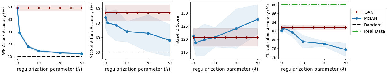
(a) Fashion-MNIST

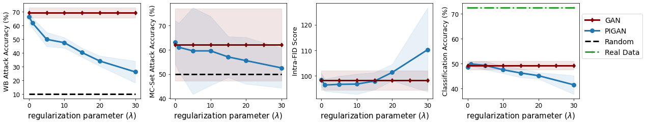
(b) CIFAR 10

Figure 1: Privacy and fidelity measures for PIGAN trained with $N=2$ and various regularization $\lambda$.

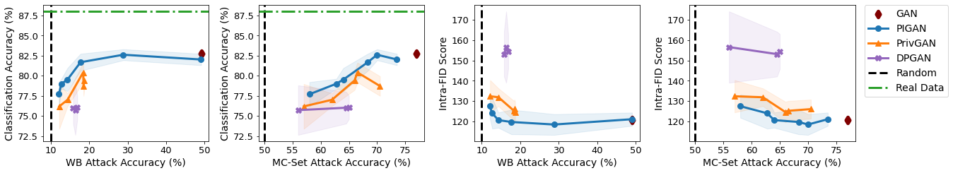
(a) Fashion-MNIST

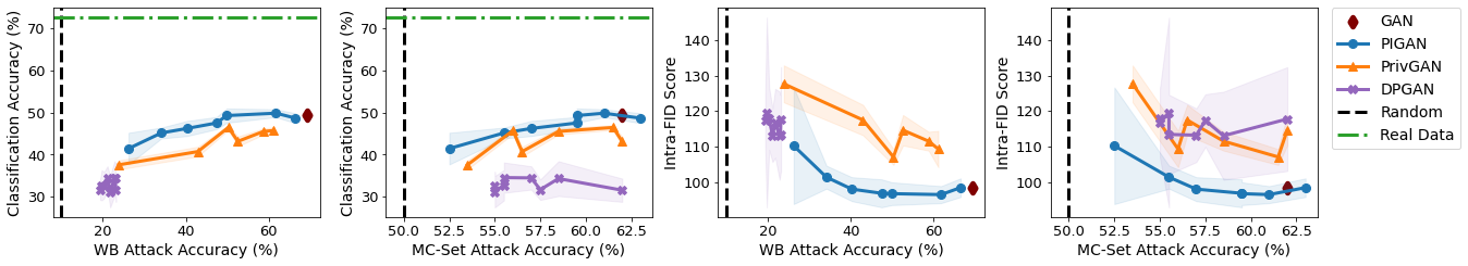
(b) CIFAR 10

Figure 2: Privacy-fidelity trade-off achieved with different private models.

5.2.2 White box attacks using discriminator confidence scores

As pointed out in (Mukherjee et al., 2021), GANs can be visually compared in terms of their resistance to WB attacks based on the distribution of confidence scores predicted by the discriminator on train and holdout samples. For a generative model with better privacy protection, the distributions will be more similar and the statistical differences between scores assigned to train and non-train (holdout) samples can not be exploited by an adversary. As shown in Fig. 3, the distributions for non-private GAN are very different, while they they overlap more for PIGAN as regularization parameter $\lambda$ is increased.

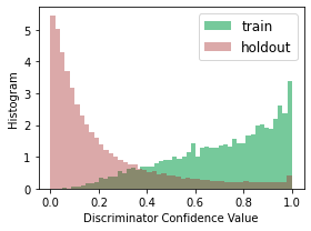
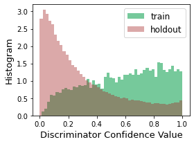
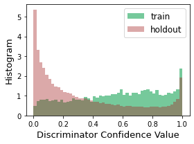
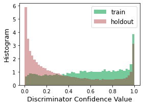
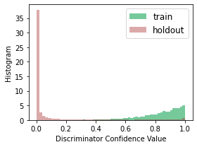
(a) GAN

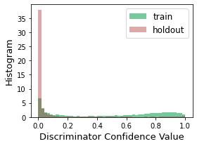
(b) PIGAN ($\lambda=1$)

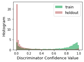
(c) PIGAN ($\lambda=10$)

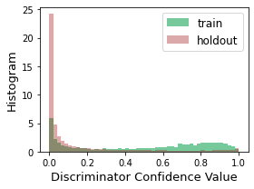
(d) PIGAN ($\lambda=20$)

Figure 3: Distribution of PIGAN’s discriminator confidence score on train and holdout data compared to non-private GAN for Fashion-MNIST (top) and CIFAR-10 (bottom).

	Fashion-MNIST				CIFAR-10
	PIGAN	PrivGAN	DPGAN		PIGAN	PrivGAN	DPGAN
WB attack ($\%$) $\downarrow$	17.7$\pm$1.1	18.3$\pm$1.3	16.9$\pm$0.9		26.2$\pm$7.8	23.8$\pm$6.8	23.0$\pm$5.4
MC-Set attack ($\%$) $\downarrow$	68.3$\pm$10.9	67.0$\pm$12.5	65.0$\pm$9.2		52.5$\pm$8.2	53.5$\pm$12.6	55.5$\pm$9.12
Inception Score $\uparrow$	2.43$\pm$0.03	2.40$\pm$0.03	2.19$\pm$0.08		3.92$\pm$0.16	3.62$\pm$0.22	3.49$\pm$0.15
FID Score $\downarrow$	22.8$\pm$1.57	33.9$\pm$1.3	46.1$\pm$7.4		70.44$\pm$15.3	87.6$\pm$7.8	75.4$\pm$9.2
Intra-FID Score $\downarrow$	119.7$\pm$6.04	125.2$\pm$4.8	154.4$\pm$8.6		110.2$\pm$16.4	127.4$\pm$5.2	113.4$\pm$11.2
Classification Accuracy ($\%$) $\uparrow$	81.7$\pm$1.1	79.6$\pm$1.7	76.1$\pm$1.4		41.4$\pm$3.7	37.6$\pm$1.1	34.6$\pm$3.6

Table 1: Comparison of privacy-preserving models trained to achieve similar WB attack accuracy levels.

	Privacy Attacks					Fidelity Scores
	WB $\downarrow$	TVD $\downarrow$	MC-Set $\downarrow$	MC-Single $\downarrow$		Inception $\uparrow$	FID $\downarrow$	Intra-FID $\downarrow$	Classification $\uparrow$
$N=2$	28.8$\pm$1.5	0.448$\pm$0.015	70.0$\pm$7.7	51.8$\pm$0.8		2.44$\pm$0.03	20.7$\pm$1.2	118.5$\pm$5.1	82.6$\pm$0.6
$N=3$	18.5$\pm$1.9	0.422$\pm$0.016	63.9$\pm$10.6	51.4$\pm$0.6		2.43$\pm$0.04	24.2$\pm$1.8	120.1$\pm$3.2	81.5$\pm$0.1
$N=4$	22.7$\pm$2.6	0.461$\pm$0.024	65.5$\pm$11.5	51.8$\pm$0.9		2.45$\pm$0.06	24.4$\pm$1.3	120.7$\pm$4.3	81.9$\pm$0.5
$N=5$	21.3$\pm$2.7	0.455$\pm$0.025	64.5$\pm$9.3	51.6$\pm$0.6		2.34$\pm$0.04	22.9$\pm$1.7	125.1$\pm$4.8	82.2$\pm$0.7
$N=6$	22.3$\pm$2.8	0.458$\pm$0.027	69.5$\pm$3.5	51.9$\pm$1.1		2.44$\pm$0.03	25.7$\pm$2.1	119.4$\pm$4.6	81.5$\pm$0.8

Table 2: Privacy and fidelity measures of PIGAN trained with $\lambda=1$ and different $N$ on Fashion-MNIST.

5.2.3 Privacy-Fidelity Trade-off

To simultaneously compare the privacy loss and generated sample quality achieved by PIGAN ($N=2$) with the baselines (GAN, PrivGAN ($N=2$) and DPGAN), we use the trade-off curves presented in Fig. 2. The curves are generated by training PIGAN and PrivGAN for a range of $\lambda$ and by training DPGAN for a range of $\epsilon$ obtained from different clipping and noise levels. For Fashion-MNIST and CIFAR-10, the two left curves in Figs. 2 (a) and (b) are strictly higher (other than one point for CIFAR-10) than the curves of all other private methods, and the two right curves are strictly lower. Therefore, for a specified level of privacy (i.e., a fixed point on the $x$-axis), a classifier trained on data that is generated by PIGAN will generalize better compared to one trained on data generated by other private models. Moreover, based on the lower Intra-FID scores shown in two right curves in Figs. 2 (a) and (b), PIGAN is able to generate data with better sample quality and higher intra-class diversity. As expected for differentially private GANs, DPGAN is inferior to PIGAN and PrivGAN for both datasets, and provides privacy at the cost of losing on downstream utility and generated sample quality. The models are compared visually based on generated sample quality in Appendix B.2.

Table 2 reports the different fidelity metrics for each model based on a fixed WB accuracy point on the curves in Fig. 2, i.e., when the models are trained (with proper parameters $\lambda$, $\epsilon$) to achieve (almost) equal WB attack accuracy. Specifically, considering WB attack accuracy close to $17\%$ for Fashion-MNIST, PIGAN ($\lambda=5$) outperforms PrivGAN ($\lambda=0.01$) and DPGAN by $2.1\%$ and $5.6\%$ in terms of downstream classification, and by $5.5$ and $34.7$ in terms of Intra-FID score, respectively. For CIFAR-10, when considering WB attack success of around $23$-$26\%$, PIGAN ($\lambda=30$) generates data with $3.8\%$ and $6.8\%$ higher classification utility compared to PrivGAN ($\lambda=20$) and DPGAN, respectively.

5.2.4 Hyperparameter ${N}$

In theory, increasing $N$ should improve privacy since the classifier $Q$ would prevent the generative model from overfitting to specific subsets of the data. However, larger $N$ results in less training samples for each membership group, which impacts the learned generative distribution for each group and the resulting sample quality. Privacy and fidelity measures for PIGAN trained on Fashion-MNIST for $\lambda=1$ are reported in Table 2 as $N$, the cardinality of latent code $\mathbf{c}$, is changed from $2$ to $6$. An equal train set size is used for training PIGAN with different $N$. Increasing $N$ from $2$ to $3$ reduces the success of WB and MC-Set attacks by $10.3\%$ and $6.1\%$, respectively. This improvement in privacy only degrades the Intra-FID score by $1.6$ points and the classification performance by $1.1\%$. Increasing $N$ beyond $3$ does not seem to improve the privacy-utility trade-off on Fashion-MNIST considerably. Parameters $N$ and $\lambda$ are hyper-parameters that can be tuned for the downstream task, and will likely depend on the dataset as mentioned by (Mukherjee et al. 2021) based on experiments for PrivGAN.

5.2.5 Training Efficiency of PIGAN

We empirically demonstrate that the proposed PIGAN model can be trained more efficiently compared to PrivGAN, which requires training multiple generator-discriminator pairs.The following table summarizes the number of trainable parameters in each model. Compared to the GAN architecture, PIGAN has $1.33\times$ more parameters when trained on Fashion-MNIST, while PrivGAN has $2.28\times$ more parameters.

	$\#$parameters ($\times 10^{6}$)
	GAN	PIGAN	PrivGAN
Fashion-MNIST	2.24	2.98	5.11
CIFAR-10	1.93	2.59	4.39

As opposed to PIGAN, the number of parameters in PrivGAN increases (almost linearly) with $N$, and each generator-discriminator pair in PrivGAN is trained with a smaller fraction of the data. The training procedure for PrivGAN is such that each generator-discriminator pair is only trained on $1/N^{\text{th}}$ of the training data. Therefore, for equal batch size and number of epochs, PrivGAN parameters are updated less compared to PIGAN. We conduct the following two experiments to compare the models in terms of training efficiency, and report the results in Table 3. In both experiments, $N=2$ and $\lambda$ is chosen such that PIGAN generates samples with relatively similar (or slightly stronger) privacy levels compared to PrivGAN in terms of WB attack accuracy. Note that for this choice of $\lambda$, PrivGAN has lower vulnerability to MC-Set attacks compared to PIGAN.

Experiment 1:

We trained PIGAN for less number of epochs compared to PrivGAN. For Fashion-MNIST, PIGAN was trained for $200$ epochs (with $K=100$), while PrivGAN was trained for 300 epochs. For CIFAR-10 we used $400$ epochs (with $K=300$) for PIGAN compared to $500$ epochs for PrivGAN. As observed from Table 3(a), when the models are trained to achieve similar levels of privacy in terms of WB attacks, PIGAN outperforms PrivGAN in terms of generated sample fidelity despite being trained for less epochs.

Experiment 2:

We trained PIGAN on $3/4^{\text{th}}$ of the train set on both Fashion-MNIST and CIFAR-10 datasets, while we trained PrivGAN on the entire train set. From Table 3(b), it can be observed that even with $25\%$ less training samples, PIGAN is able to generate images with higher (or similar) quality in terms of classification accuracy and Intra-FID score, while providing WB privacy levels comparable to PrivGAN for both datasets.

	Fashion-MNIST			CIFAR-10
	PIGAN	PrivGAN		PIGAN	PrivGAN
WB ($\%$) $\downarrow$	13.9$\pm$0.7	14.3$\pm$0.8		30.9$\pm$3.9	42.9$\pm$6.8
MC-Set ($\%$) $\downarrow$	64.5$\pm$0.7	62.0$\pm$11.7		59.5$\pm$10.6	56.5$\pm$8.4
Intra-FID $\downarrow$	119.5$\pm$4.6	131.9$\pm$4.4		96.9$\pm$3.3	117.5$\pm$4.3
Classification Accuracy ($\%$) $\uparrow$	80.2$\pm$0.8	77.0$\pm$0.8		45.3$\pm$1.4	40.7$\pm$1.2

(a) Experiment 1

	Fashion-MNIST			CIFAR-10
	PIGAN	PrivGAN		PIGAN	PrivGAN
WB ($\%$) $\downarrow$	12.0$\pm$0.3	12.2$\pm$0.5		39.8$\pm$2.7	42.9$\pm$6.8
MC-Set ($\%$) $\downarrow$	62.1$\pm$13.1	57.0$\pm$8.7		59.0$\pm$11.5	56.5$\pm$8.4
Intra-FID $\downarrow$	122.2$\pm$7.0	132.4$\pm$7.9		100.1$\pm$3.1	117.5$\pm$4.3
Classification Accuracy ($\%$) $\uparrow$	77.1$\pm$0.9	76.2$\pm$2.8		43.0$\pm$1.7	40.7$\pm$1.2

(b) Experiment 2

Table 3: PIGAN vs PrivGAN in terms of training efficiency.

5.2.6 Privacy Range

As observed from Fig. 2, PIGAN provides a wider privacy range against WB attacks compared to PrivGAN (as also noted in (Mukherjee et al., 2021)) and DPGAN, especially for Fashion-MNIST. It is worth noting that PrivGAN requires training multiple G-D pairs with a more trainable parameters compared to PIGAN, and therefore, it requires more training data and updates compared to PIGAN, especially for large values of $N$. PrivGAN’s smaller privacy range, may potentially be due to the additional computational cost, since all $N$ G-D pairs may not converge as fast as models with a single generator and discriminator (e.g., GAN and PIGAN) when trained for the same number of iterations. Consequently, it may be less susceptible to privacy attacks due to less fitting to the data. Based on the results reported in Fig. 2, without regularization ($\lambda=0$), PrivGAN is $30.7\%$ and $31.4\%$ less susceptible to WB attacks compared to non-private GAN for Fashion-MNIST and CIFAR-10, respectively. However, as expected, with no privacy regularization using $\lambda=0$, PIGAN achieves almost the same WB attack accuracy as non-private GAN.

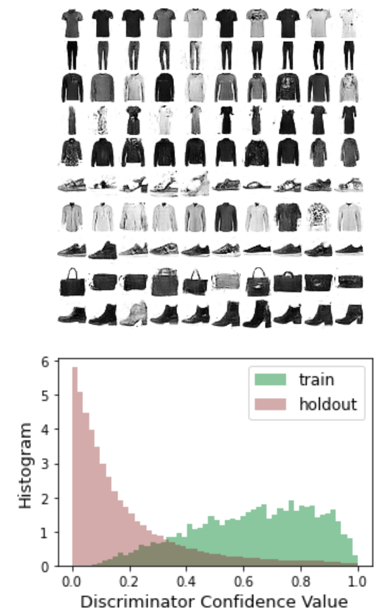
(a) $\mathbf{c}=1$

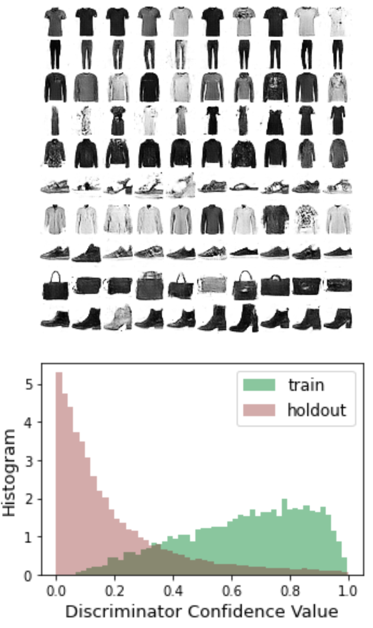
(b) $\mathbf{c}=2$

Figure 4: PIGAN trained on Fashion-MNIST with $N=2$, $\lambda=0$.

5.2.7 No Penalty $\boldsymbol{\lambda=0}$

To further demonstrate the vulnerability of GANs to privacy attacks, we train PIGAN on Fashion-MNIST with $N=2$ and $\lambda=0$, such that the generator is conditionally trained on different subsets of the data but is not penalized for memorizing the data in each subset. As shown in Fig. 4, synthetic samples generated by PIGAN are visually indistinguishable for $\mathbf{c}=1$ and $\mathbf{c}=2$, i.e., when a GAN is trained on different subsets of the dataset. However, there is a clear distinction between the discriminator’s confidence about the realness of a sample from the train or holdout set for both values of $\mathbf{c}$. Such statistical differences arise from overfitting to the training set and can be exploited by an adversary. By imposing regularization with $\lambda=1$, the WB and MC-Set attack accuracy diminish from $49.1\%$ to $28.8\%$, and from $73.5\%$ to $70\%$, respectively (as reported in Table 2). PIGAN’s discriminator confidence score distributions are compared for various $\lambda$ in Appendix 5.2.2, which shows that the distributions become more similar as $\lambda$ is increased, meaning the discriminator assigns closer confidence values to real samples coming from train and holdout sets.

6 Conclusions

We propose a membership privacy-preserving training framework for deep generative models that mitigates overfitting to training data and leakage of sensitive information. Our proposed model, referred to as PIGAN, learns to estimate almost identical generative distributions for data with different membership, using an information-theoretic regularization term that aims to minimize the divergence between the distributions. We show that this can be implemented using a multi-class classifier at relatively low cost compared to private GANs that train multiple generators and discriminators. Our experiments demonstrate the resilience of PIGAN against several well-known MIA attacks without considerable degradation in generated data fidelity, and show that PIGAN outperforms alternative private GANs in terms of various utility measures achieving improved privacy-fidelity trade-offs. As part of our future work we plan to implement PIGAN on tabular datasets with sensitive attributes such as health-related data. Other future work includes investigating achievable privacy levels when the information-theoretic regularization is imposed on discriminator confidence values rather than generated images, and comparing the mitigation of the two methods against various privacy attack types.

Disclaimer

This paper was prepared for informational purposes by the Artificial Intelligence Research group of JPMorgan Chase & Co. and its affiliates (“JP Morgan”), and is not a product of the Research Department of JP Morgan. JP Morgan makes no representation and warranty whatsoever and disclaims all liability, for the completeness, accuracy or reliability of the information contained herein. This document is not intended as investment research or investment advice, or a recommendation, offer or solicitation for the purchase or sale of any security, financial instrument, financial product or service, or to be used in any way for evaluating the merits of participating in any transaction, and shall not constitute a solicitation under any jurisdiction or to any person, if such solicitation under such jurisdiction or to such person would be unlawful.

Appendix

Appendix A Experimental Settings

All experiments are implemented in Keras and run with a single NVIDIA T4 GPU on an Amazon Web Services g4dn.4xlarge instance.

A.1 Model Architectures

The proposed privacy preservation framework is independent of the architecture and should generalize to alternative models, particularly more complex models that generate higher fidelity samples since they would be more susceptible to MIAs (Hayes et al., 2019). However, since the focus of our work is privacy-preserving techniques, we follow existing work in this area (Hayes et al., 2019; Hilprecht et al., 2019; Mukherjee et al., 2021; Xie et al., 2018) and adopt the deep convolutional generative adversarial network (DCGAN) (Radford et al., 2015) as our base architecture and we compare various privacy-preserving techniques for the same architecture. Models are implemented in their conditional format to provide control over the generated class labels. All models are trained for $300$ epochs on Fashion-MNIST and $500$ epochs on CIFAR-10, and we use the Adam optimizer (Kingma & Ba, 2014) with learning rate $\alpha=0.0002$ and momentum $\beta_{1}=0.5$, and a batch size of $128$. The generator and discriminator architectures for non-private GAN are presented in Table 4. We use BN to denote batch normalization with momentum $0.9$, and LReLU to denote Leaky Rectified Unit with slope $\alpha=0.2$. The noise vector $\mathbf{z}$ is generated from a normal distribution with dimension $n_{z}=100$ for both Fashion-MNIST and CIFAR-10. Table 5 provides the architectures used for PIGAN, which have been modified compared to their non-private counterparts to take the latent code $\mathbf{c}$ as an additional input, which is concatenated with other inputs in the early layers. Classifier $Q(\mathbf{x})$ is implemented using a very similar architecture as the non-private discriminator with the difference that it does not take the class labels $\mathbf{y}$ as input and that a Softmax activation is used in the final layer instead of a Sigmoid. For PrivGAN (Mukherjee et al., 2021), all generator-discriminator pairs use the same architecture as non-private GAN, and the privacy discriminator is implemented identical to the classifier of PIGAN. DPGAN is implemented with the same architecture as non-private GAN and trained with differential privacy for $\delta=1e^{-4}$. For CIFAR-10, we use one-sided label smoothing for the discriminators by using a target label of $0.9$ rather than $1$.

A.2 Other Design Choices and Hyperparameters

For both PIGAN and PrivGAN, we initialize classifier $Q$ and the privacy discriminator with weights obtained from pre-training them for $50$ epochs on the training data using membership indices as class labels. Additionally, the discriminators and generators of PrivGAN are trained for $K=100$ epochs without training the privacy discriminator (Mukherjee et al., 2021), while for PIGAN, they are trained for $K=200$ epochs on Fashion-MNIST and $K=400$ epochs on CIFAR-10, without updating the classifier.

When evaluating the fidelity of data generated by the models, we use Tensorflow implementations of the Inception score and Fréchet Inception Distance, provided in https://github.com/tsc2017/Inception-Score and https://github.com/tsc2017/Frechet-Inception-Distance. We use $10^{4}$ generated samples for evaluations on Fashion-MNIST and $2\times 10^{4}$ generated samples for CIFAR-10. The classifier architectures used for evaluating the models based on downstream task performance is summarized in Table 6. MaxPool denotes a maxpool layer with pooling size of $2\times 2$. The classifiers are trained with the Adam optimizer (learning rate $\alpha=0.0002$ and momentum $\beta_{1}=0.5$), for $50$ epochs and a batch size of $64$ for both Fashion-MNIST and CIFAR-10.

	Generator $G(\mathbf{z},\mathbf{y})$		Discriminator $D(\mathbf{x},\mathbf{y})$
Inputs	$\mathbf{z}\sim\mathcal{N}(0,\mathbf{I})$ and $\mathbf{y}\in\{1,\dots,10\}$		$\mathbf{x}\sim\mathbb{R}^{28\times 28\times 1}$ and $\mathbf{y}\in\{1,\dots,10\}$
Layers	Concatenate $\mathbf{z}$ and $\mathbf{y}$		Dense $28\times 28$, Reshape ($\mathbf{y}$ $\rightarrow$ $\mathbf{\hat{y}}$)
	Dense $7\times 7\times 128$, BN, LReLU, Reshape		Concatenate $\mathbf{x}$ and $\mathbf{\hat{y}}$
	$5\times 5$ stride=$2$ Deconv $128$, BN, LReLU		$5\times 5$ stride=$2$ Conv $64$, LReLU
	$5\times 5$ stride=$2$ Deconv $128$, BN, LReLU		$5\times 5$ stride=$2$ Conv 128, LReLU
	$3\times 3$ stride=$1$ Deconv $64$, BN, LReLU		$5\times 5$ stride=$2$ Conv 128, LReLU, Flatten
	$3\times 3$ stride=$1$ Conv $1$, Tanh		Dense $1$, Sigmoid

(a) Fashion-MNIST

	Generator $G(\mathbf{z},\mathbf{y})$		Discriminator $D(\mathbf{x},\mathbf{y})$
Inputs	$\mathbf{z}\sim\mathcal{N}(0,\mathbf{I})$ and $\mathbf{y}\in\{1,\dots,10\}$		$\mathbf{x}\sim\mathbb{R}^{32\times 32\times 3}$ and $\mathbf{y}\in\{1,\dots,10\}$
Layers	Concatenate $\mathbf{z}$ and $\mathbf{y}$		$3\times 3$ stride=$1$ Conv $64$, LReLU ($\mathbf{x}$ $\rightarrow$ $\mathbf{\hat{x}}$)
	Dense $4\times 4\times 256$, LReLU, Reshape		Dense $32\times 32\times 3$, Reshape ($\mathbf{y}$ $\rightarrow$ $\mathbf{\hat{y}}$)
	$4\times 4$ stride=$2$ Deconv $128$, LReLU		Concatenate $\mathbf{\hat{x}}$ and $\mathbf{\hat{y}}$
	$4\times 4$ stride=$2$ Deconv $128$, LReLU		$3\times 3$ stride=$2$ Conv $128$, LReLU
	$4\times 4$ stride=$2$ Deconv $64$, LReLU		$3\times 3$ stride=$2$ Conv $128$, LReLU
	$3\times 3$ stride=$1$ Conv $3$, Tanh		$3\times 3$ stride=$2$ Conv $256$, LReLU, Flatten
			Dense $1$, Sigmoid

(b) CIFAR-10

Table 4: Non-private GAN generator and discriminator architectures.

Generator $G(\mathbf{z},\mathbf{c},\mathbf{y})$ Discriminator $D(\mathbf{x},\mathbf{c},\mathbf{y})$ Classifier $Q(\mathbf{x})$ Inputs $\mathbf{z}\sim\mathcal{N}(0,\mathbf{I})$, $\mathbf{y}\in\{1,\dots,10\}$ $\mathbf{x}\sim\mathbb{R}^{28\times 28\times 1}$, $\mathbf{y}\in\{1,\dots,10\}$ $\mathbf{x}\sim\mathbb{R}^{28\times 28\times 1}$ and $\mathbf{c}\sim\text{Uniform}\{1,N\}$ and $\mathbf{c}\sim\text{Uniform}\{1,N\}$ Layers Concatenate $\mathbf{z}$ and $\mathbf{y}$ ($\mathbf{z}$, $\mathbf{y}$ $\rightarrow$ $\mathbf{z}\mathbf{y}$) Dense $28\times 28\times 1$, Reshape ($\mathbf{y}$ $\rightarrow$ $\mathbf{\hat{y}}$) $5\times 5$ stride=$2$ Conv $64$, LReLU Dense $7\times 7\times 128$ ($\mathbf{z}\mathbf{y}$ $\rightarrow$ $\widehat{\mathbf{z}\mathbf{y}}$) Dense $28\times 28\times 1$, Reshape ($\mathbf{c}$ $\rightarrow$ $\mathbf{\hat{c}}$) $5\times 5$ stride=$2$ Conv 128, LReLU Dense $7\times 7\times 32$ ($\mathbf{c}$ $\rightarrow$ $\mathbf{\hat{c}}$) Concatenate $\mathbf{x}$, $\mathbf{\hat{c}}$ and $\mathbf{\hat{y}}$ $5\times 5$ stride=$2$ Conv 128, LReLU, Flatten Concatenate $\widehat{\mathbf{z}\mathbf{y}}$ and $\mathbf{\hat{c}}$, BN, LReLU, Reshape $5\times 5$ stride=$2$ Conv $64$, LReLU Dense $N$, Softmax $5\times 5$ stride=$2$ Deconv $128$, BN, LReLU $5\times 5$ stride=$2$ Conv 128, LReLU $5\times 5$ stride=$2$ Deconv $128$, BN, LReLU $5\times 5$ stride=$2$ Conv 128, LReLU, Flatten $3\times 3$ stride=$1$ Deconv $64$, BN, LReLU Dense $1$, Sigmoid $3\times 3$ stride=$1$ Conv $1$, Tanh

(a) Fashion-MNIST

Generator $G(\mathbf{z},\mathbf{c},\mathbf{y})$ Discriminator $D(\mathbf{x},\mathbf{c},\mathbf{y})$ Classifier $Q(\mathbf{x})$ Inputs $\mathbf{z}\sim\mathcal{N}(0,\mathbf{I})$, $\mathbf{y}\in\{1,\dots,10\}$ $\mathbf{x}\sim\mathbb{R}^{32\times 32\times 3}$, $\mathbf{y}\in\{1,\dots,10\}$ $\mathbf{x}\sim\mathbb{R}^{32\times 32\times 3}$ and $\mathbf{c}\sim\text{Uniform}\{1,N\}$ and $\mathbf{c}\sim\text{Uniform}\{1,N\}$ Layers Concatenate $\mathbf{z}$ and $\mathbf{y}$ ($\mathbf{z}$, $\mathbf{y}$ $\rightarrow$ $\mathbf{z}\mathbf{y}$) $3\times 3$ stride=$1$ Conv $64$, LReLU ($\mathbf{x}$ $\rightarrow$ $\mathbf{\hat{x}}$) $3\times 3$ stride=$1$ Conv $64$, LReLU Dense $4\times 4\times 256$, Reshape ($\mathbf{z}\mathbf{y}$ $\rightarrow$ $\widehat{\mathbf{z}\mathbf{y}}$) Dense $32\times 32\times 3$, Reshape ($\mathbf{y}$ $\rightarrow$ $\mathbf{\hat{y}}$) $3\times 3$ stride=$2$ Conv $128$, LReLU Dense $4\times 4\times 64$, Reshape ($\mathbf{c}$ $\rightarrow$ $\mathbf{\hat{c}}$) Dense $32\times 32\times 1$, Reshape ($\mathbf{c}$ $\rightarrow$ $\mathbf{\hat{c}}$) $3\times 3$ stride=$2$ Conv $128$, LReLU Concatenate $\widehat{\mathbf{z}\mathbf{y}}$ and $\mathbf{\hat{c}}$, LReLU Concatenate $\mathbf{x}$, $\mathbf{\hat{c}}$ and $\mathbf{\hat{y}}$ $3\times 3$ stride=$2$ Conv $256$, LReLU, Flatten $4\times 4$ stride=$2$ Deconv $128$, LReLU $3\times 3$ stride=$2$ Conv $128$, LReLU Dense $N$, Softmax $4\times 4$ stride=$2$ Deconv $128$, LReLU $3\times 3$ stride=$2$ Conv $128$, LReLU $4\times 4$ stride=$2$ Deconv $64$, LReLU $3\times 3$ stride=$2$ Conv $256$, LReLU, Flatten $3\times 3$ stride=$1$ Conv $3$, Tanh Dense $1$, Sigmoid

(b) CIFAR-10

Table 5: PIGAN generator, discriminator and classifier architectures.

	Fashion-MNIST		CIFAR-10
Inputs	$\mathbf{x}\sim\mathbb{R}^{28\times 28\times 1}$ and $\mathbf{y}\in\{1,\dots,10\}$		$\mathbf{x}\sim\mathbb{R}^{32\times 32\times 3}$ and $\mathbf{y}\in\{1,\dots,10\}$
Layers	$3\times 3$ stride=$1$ Conv $32$, ReLU		$3\times 3$ stride=$1$ Conv $32$, ReLU
	$3\times 3$ stride=$1$ Conv $64$, ReLU, MaxPool, Dropout($0.5$)		$3\times 3$ stride=$1$ Conv $32$, ReLU, MaxPool, Dropout($0.2$)
	$3\times 3$ stride=$1$ Conv $128$, ReLU, MaxPool, Dropout($0.5$), Flatten		$3\times 3$ stride=$1$ Conv $64$, ReLU
	Dense $128$, ReLU, Dropout($0.5$)		$3\times 3$ stride=$1$ Conv $64$, ReLU, MaxPool, Dropout($0.2$)
	Dense $10$, Softmax		$3\times 3$ stride=$1$ Conv $128$, ReLU
			$3\times 3$ stride=$1$ Conv $128$, ReLU, MaxPool, Dropout($0.3$), Flatten
			Dense $256$, ReLU, Dropout($0.3$)
			Dense $10$, Softmax

Table 6: Classifier architectures used to evaluate generative models in downstream tasks.

Appendix B Additional Results

B.1 Further evaluation of PIGAN trained with different $\boldsymbol{\lambda}$

Fig. 5 provides additional quantitative evaluation measures for PIGAN that were not presented in the main paper as the regularization parameter $\lambda$ increases. As expected, the TVD attack score, which is an upper limit on WB attack accuracy using the discriminator, is lower for larger values of $\lambda$ for both datasets. Similarly, PIGAN becomes less vulnerable to MC-Single attacks as $\lambda$ increases. Our observations from Fig. 5 regarding MC-Single attacks are aligned with the experiments in (Hilprecht et al., 2019) (also noted in (Mukherjee et al., 2021)) that MC-Single attacks are much less successful compared to MC-Set attacks and achieve accuracy close to random guessing. As $\lambda$ is increased, the FID score also increases while the inception score decreases for Fashion-MNIST, indicating the degradation in generated sample quality. When moving from $\lambda=0$ to $\lambda=1$, an initial dip in FID and rise in the Inception score is observed, which is in agreement with the small increase in classification accuracy observed in Fig. 1, confirming an improvement in generated data fidelity. A possible explanation for this improvement for very small $\lambda$ could be that the PIGAN regularization used to prevent overfitting and improve privacy is also improving the training process. The curves for CIFAR-10 exhibit similar expected trends. In Fig. 6 we visually compare the samples generated with PIGAN and observe that while for small $\lambda$ the images are comparable to non-private GAN samples, the quality gets progressively worse with larger values of $\lambda$.

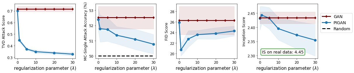
(a) Fashion-MNIST

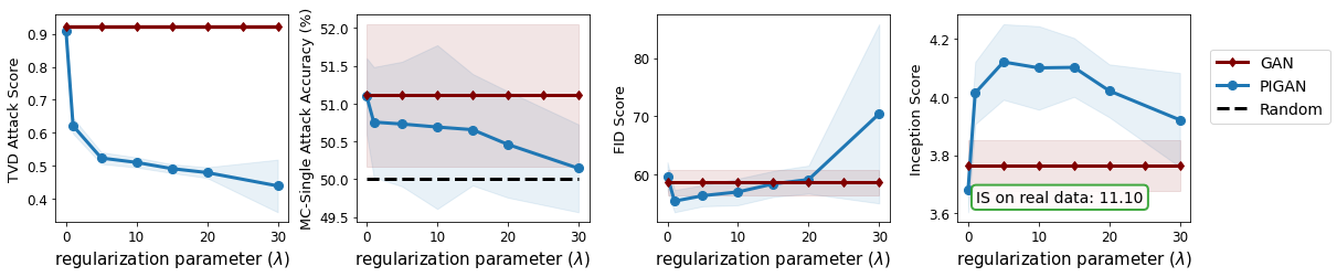
(b) CIFAR 10

Figure 5: Additional privacy and fidelity measures for PIGAN trained with $N=2$ and various regularization $\lambda$.

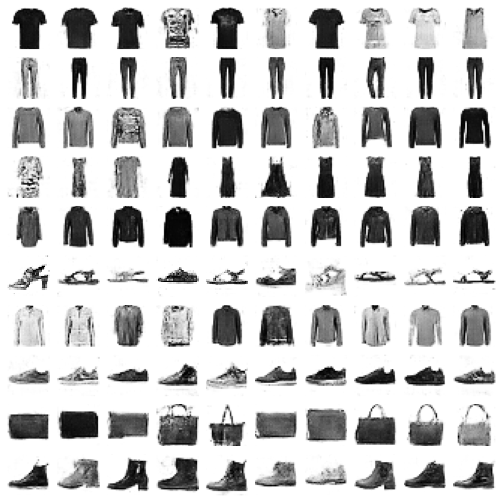
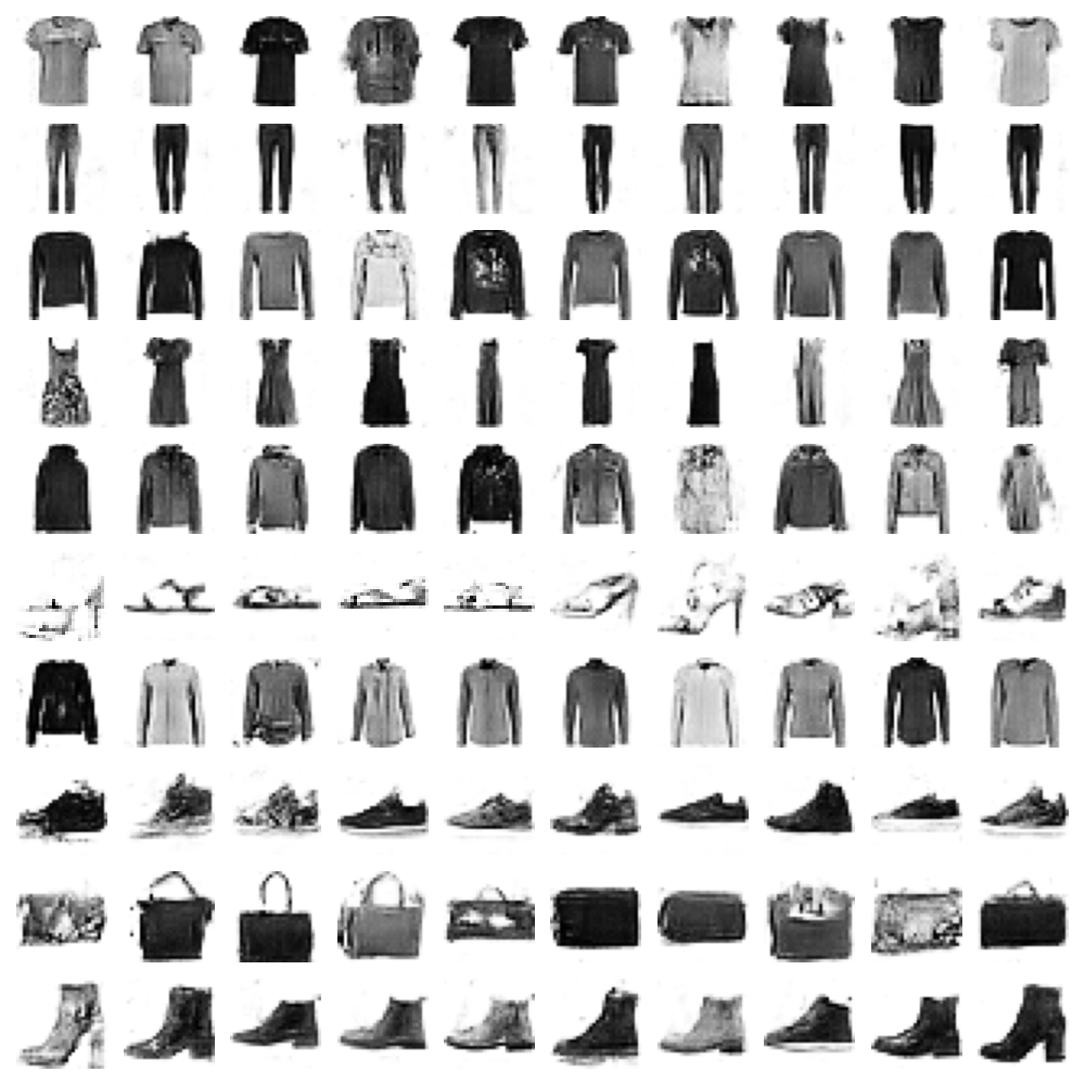
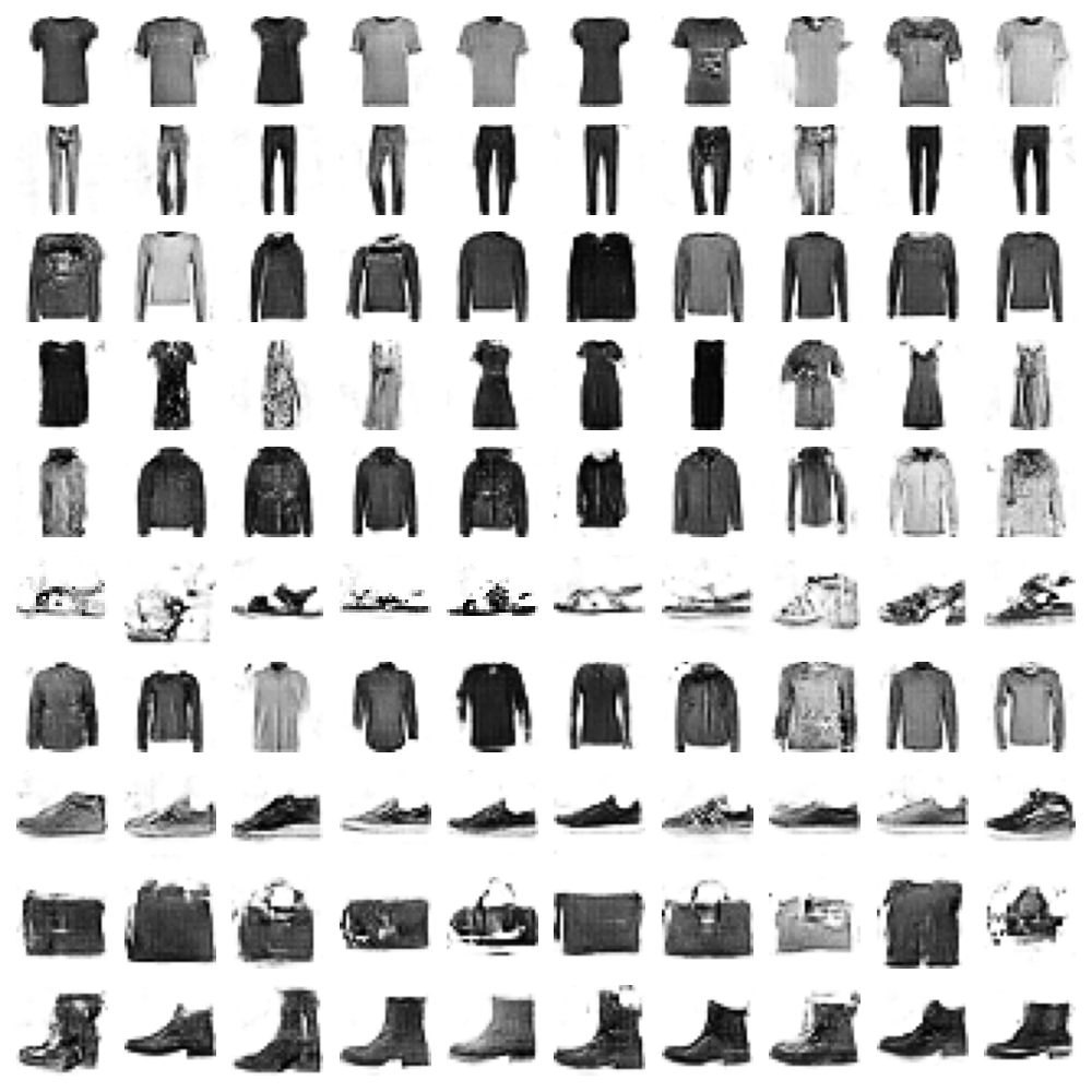
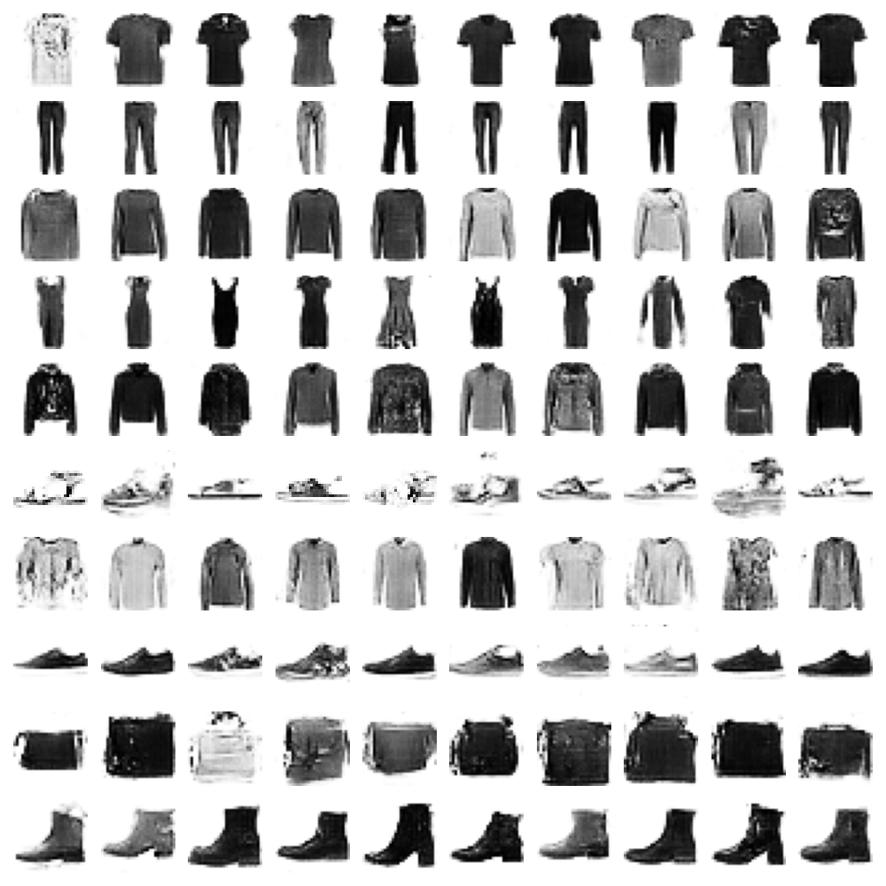
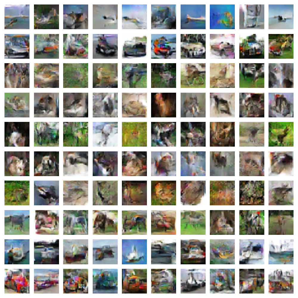
(a) GAN

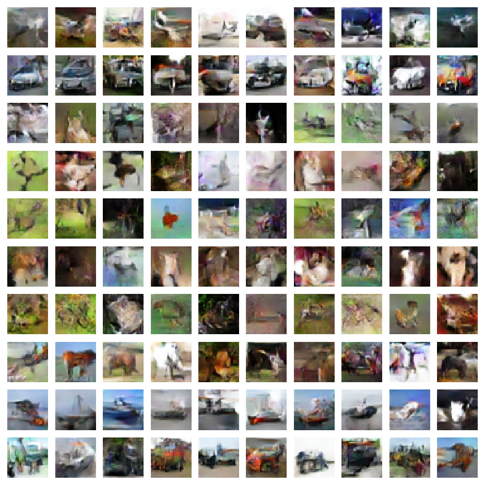
(b) PIGAN ($\lambda=1$)

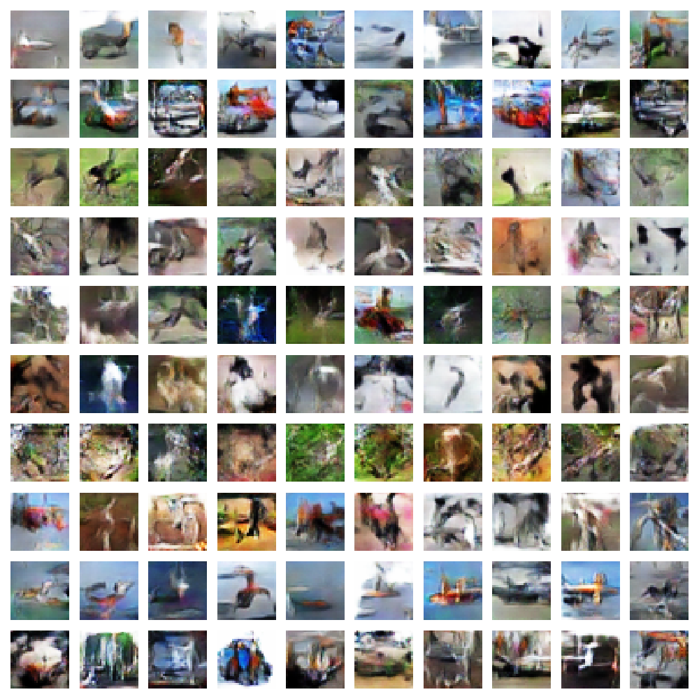
(c) PIGAN ($\lambda=10$)

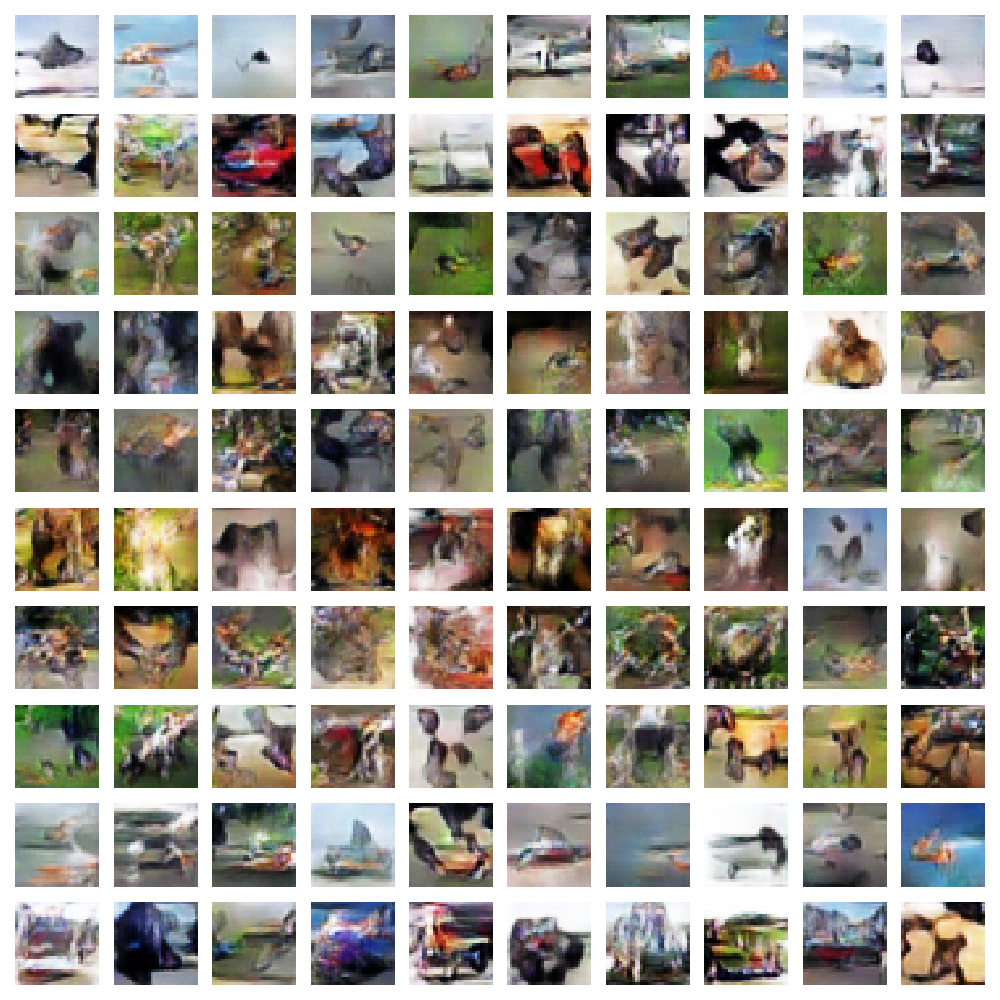
(d) PIGAN ($\lambda=20$)

Figure 6: Samples generated by PIGAN with various $\lambda$ compared to non-private GAN.

B.2 Comparison of the privacy-fidelity trade-off

In Fig. 7, we compare the different private models in terms of privacy and fidelity measures not presented in the main paper. As with the trade-offs observed in Fig. 2, the two left curves for both Fashion-MNIST and CIFAR-10 are almsot always higher than the curves of other private methods, and the two right curves are lower. It is also observed that PIGAN covers a wider privacy-level range compared to PrivGAN and especially DPGAN. For a given WB attack success rate, PIGAN is able to generate images with higher Inception score, i.e., better sample quality. Similarly, for a given MC-Set and MC-Single attack success rate, PIGAN results in better downstream classification performance and achieves lower FID and Intra-FID scores, respectively. It is worth noting that as discussed in (Borji, 2019) and (Liu et al., 2018), both IS and FID score have limitations especially when evaluating class-conditional models. While we use Intra-FID to evaluate generated image quality in our experiments, other metrics for conditional generative models include Class-Aware Fréchet Distance (CAFD) (Liu et al., 2018), Fréchet Joint Distance (FJD) (DeVries et al., 2019) and Conditional IS and Conditional FID scores (Benny et al., 2021).

We visually compare the generated sample quality of different private models in Figs. 8 and 9. For Fashion-MNIST it can be observed that PIGAN generates better samples visually mostly noticeable in categories such as sandals and bags. Samples generated with DPGAN have very poor quality especially in terms of color and item diversity. However, as expected, the discriminator distributions for DPGAN look almost identical confirming the strong privacy guarantees provided by differentially private trained models. Since we use class-conditional models in our experiments, we do not observe the mode-collapse resulting from high regularization values of $\lambda$ for PrivGAN, which was pointed out in (Mukherjee et al., 2021). From comparing the generated CIFAR-10 images in Fig. 9, we observe that despite the high regularization, PIGAN is able to generate images resembling those generated by non-private GAN in some of the categories, while PrivGAN generates images with lower quality overall. DPGAN is not able to generate images with reasonable visual quality, and as in Fashion-MNIST there is much less diversity in terms of color and objects within each class.

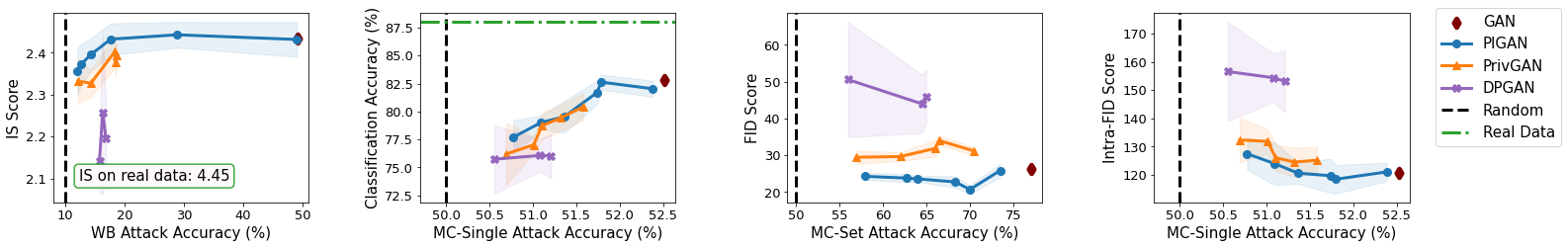
(a) Fashion-MNIST

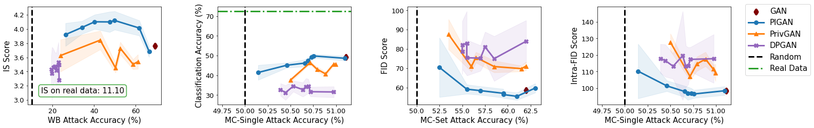
(b) CIFAR-10

Figure 7: Privacy-fidelity trade-off achieved with different private models.

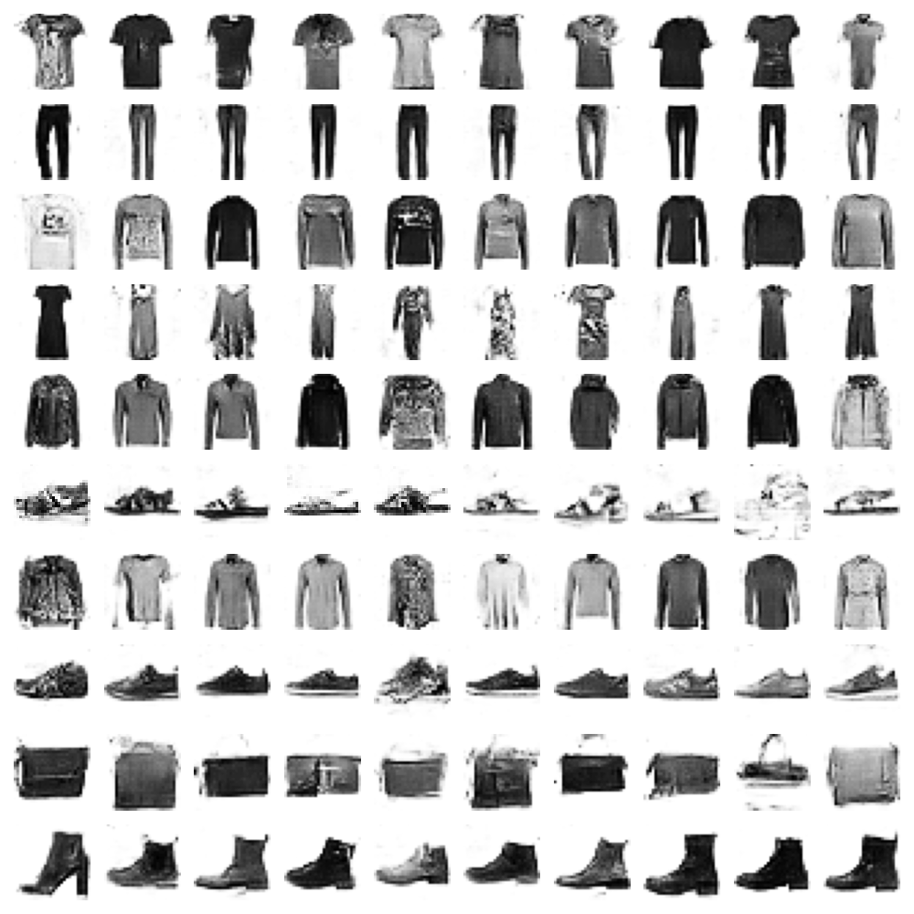
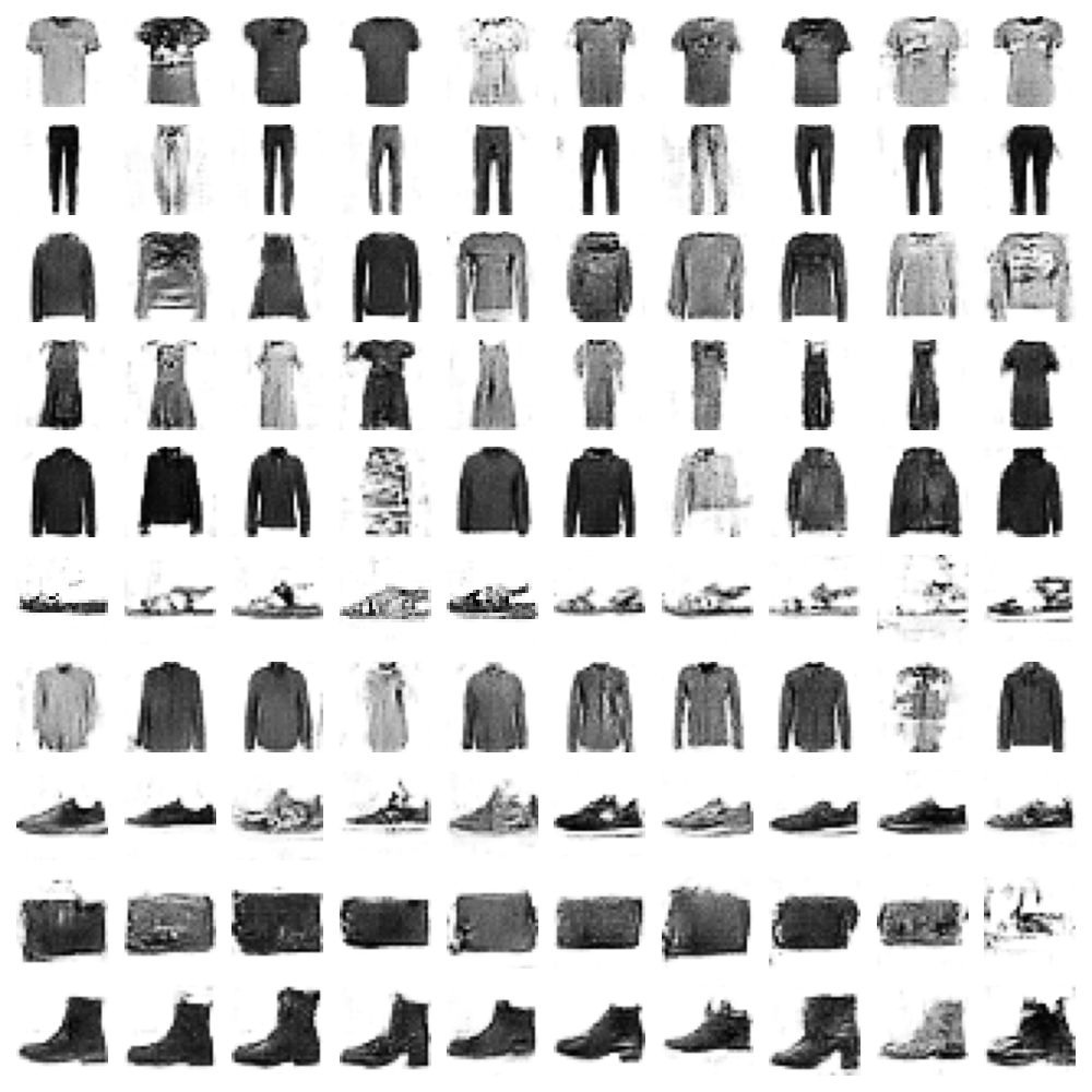
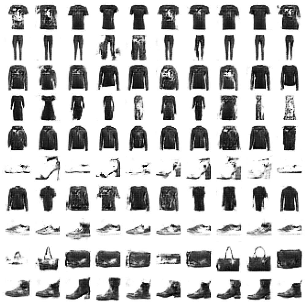
(a) GAN

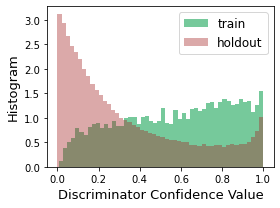
(b) PIGAN ($\lambda=5$)

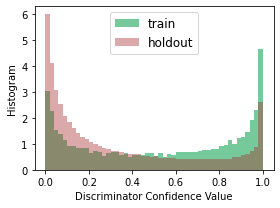
(c) PrivGAN ($\lambda=0.1$)

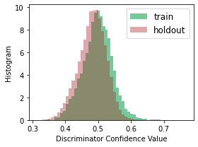
(d) DPGAN ($\sigma^{2}=0.5,c_{p}=1.2$)

Figure 8: Fashion-MNIST: Comparison between private models in terms of generated sample quality and discriminator confidence score distribution. Models are trained to achieve similar WB attack accuracy reported in Table 2.

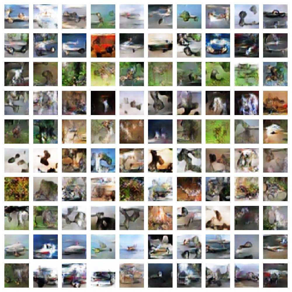
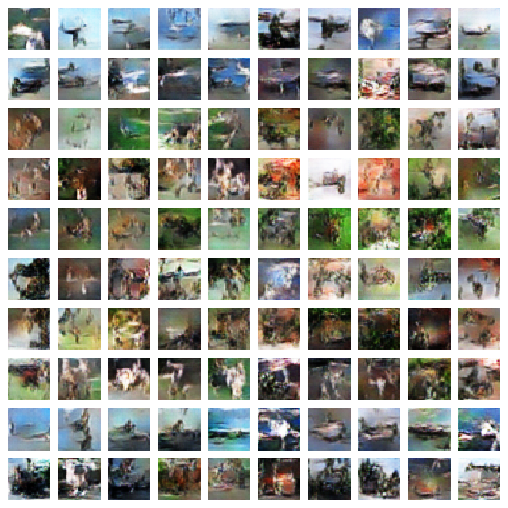
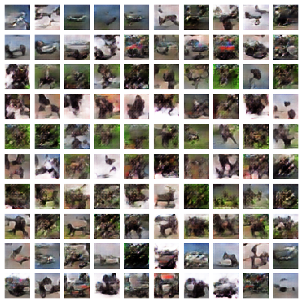
(a) GAN

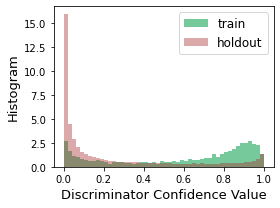
(b) PIGAN ($\lambda=30$)

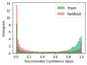
(c) PrivGAN ($\lambda=20$)

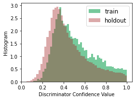
(d) DPGAN ($\sigma^{2}=0.7,c_{p}=1.5$)

Figure 9: CIFAR-10: Comparison between private models in terms of generated sample quality and discriminator confidence score distribution. Models are trained to achieve similar WB attack accuracy reported in Table 2.

References

- Arjovsky et al. (2017) Arjovsky, M., Chintala, S., and Bottou, L. Wasserstein generative adversarial networks. In International conference on machine learning, pp. 214–223. PMLR, 2017.
- Benny et al. (2021) Benny, Y., Galanti, T., Benaim, S., and Wolf, L. Evaluation metrics for conditional image generation. International Journal of Computer Vision, 129(5):1712–1731, 2021.
- Borji (2019) Borji, A. Pros and cons of gan evaluation measures. Computer Vision and Image Understanding, 179:41–65, 2019.
- Brock et al. (2019) Brock, A., Donahue, J., and Simonyan, K. Large scale GAN training for high fidelity natural image synthesis. In 7th International Conference on Learning Representations, ICLR 2019, 2019.
- Chen et al. (2020a) Chen, D., Orekondy, T., and Fritz, M. Gs-wgan: A gradient-sanitized approach for learning differentially private generators. arXiv preprint arXiv:2006.08265, 2020a.
- Chen et al. (2020b) Chen, D., Yu, N., Zhang, Y., and Fritz, M. Gan-leaks: A taxonomy of membership inference attacks against generative models. In Proceedings of the 2020 ACM SIGSAC conference on computer and communications security, pp. 343–362, 2020b.
- Chen et al. (2016) Chen, X., Duan, Y., Houthooft, R., Schulman, J., Sutskever, I., and Abbeel, P. Infogan: Interpretable representation learning by information maximizing generative adversarial nets. In Proceedings of the 30th International Conference on Neural Information Processing Systems, pp. 2180–2188, 2016.
- DeVries et al. (2019) DeVries, T., Romero, A., Pineda, L., Taylor, G. W., and Drozdzal, M. On the evaluation of conditional gans. arXiv preprint arXiv:1907.08175, 2019.
- Goodfellow et al. (2014) Goodfellow, I., Pouget-Abadie, J., Mirza, M., Xu, B., Warde-Farley, D., Ozair, S., Courville, A., and Bengio, Y. Generative adversarial nets. Advances in neural information processing systems, 27, 2014.
- Hayes et al. (2019) Hayes, J., Melis, L., Danezis, G., and De Cristofaro, E. Logan: Membership inference attacks against generative models. Proceedings on Privacy Enhancing Technologies, 2019(1):133–152, 2019.
- Heusel et al. (2017) Heusel, M., Ramsauer, H., Unterthiner, T., Nessler, B., and Hochreiter, S. Gans trained by a two time-scale update rule converge to a local nash equilibrium. Advances in neural information processing systems, 30, 2017.
- Hilprecht et al. (2019) Hilprecht, B., Härterich, M., and Bernau, D. Monte carlo and reconstruction membership inference attacks against generative models. Proceedings on Privacy Enhancing Technologies, 2019(4):232–249, 2019.
- Hinton & Salakhutdinov (2006) Hinton, G. E. and Salakhutdinov, R. R. Reducing the dimensionality of data with neural networks. science, 313(5786):504–507, 2006.
- Hitaj et al. (2017) Hitaj, B., Ateniese, G., and Perez-Cruz, F. Deep models under the gan: information leakage from collaborative deep learning. In Proceedings of the 2017 ACM SIGSAC Conference on Computer and Communications Security, pp. 603–618, 2017.
- Hoang et al. (2018) Hoang, Q., Nguyen, T. D., Le, T., and Phung, D. Mgan: Training generative adversarial nets with multiple generators. In International conference on learning representations, 2018.
- Jordon et al. (2018) Jordon, J., Yoon, J., and Van Der Schaar, M. Pate-gan: Generating synthetic data with differential privacy guarantees. In International conference on learning representations, 2018.
- Kingma & Ba (2014) Kingma, D. P. and Ba, J. Adam: A method for stochastic optimization. arXiv preprint arXiv:1412.6980, 2014.
- Kingma & Welling (2013) Kingma, D. P. and Welling, M. Auto-encoding variational bayes. In Proceedings of the 2th International Conference on Learning Representations (ICLR), 2013.
- Krizhevsky et al. (2009) Krizhevsky, A., Hinton, G., et al. Learning multiple layers of features from tiny images. 2009.
- Liu et al. (2018) Liu, S., Wei, Y., Lu, J., and Zhou, J. An improved evaluation framework for generative adversarial networks. arXiv preprint arXiv:1803.07474, 2018.
- Liu et al. (2019) Liu, Y., Peng, J., James, J., and Wu, Y. Ppgan: Privacy-preserving generative adversarial network. In 2019 IEEE 25Th international conference on parallel and distributed systems (ICPADS), pp. 985–989. IEEE, 2019.
- Mirza & Osindero (2014) Mirza, M. and Osindero, S. Conditional generative adversarial nets. arXiv preprint arXiv:1411.1784, 2014.
- Miyato & Koyama (2018) Miyato, T. and Koyama, M. cgans with projection discriminator. arXiv preprint arXiv:1802.05637, 2018.
- Mukherjee et al. (2021) Mukherjee, S., Xu, Y., Trivedi, A., Patowary, N., and Ferres, J. L. privgan: Protecting gans from membership inference attacks at low cost to utility. Proc. Priv. Enhancing Technol., 2021(3):142–163, 2021.
- Radford et al. (2015) Radford, A., Metz, L., and Chintala, S. Unsupervised representation learning with deep convolutional generative adversarial networks. arXiv preprint arXiv:1511.06434, 2015.
- Ravuri & Vinyals (2019) Ravuri, S. and Vinyals, O. Classification accuracy score for conditional generative models. arXiv preprint arXiv:1905.10887, 2019.
- Salimans et al. (2016) Salimans, T., Goodfellow, I., Zaremba, W., Cheung, V., Radford, A., and Chen, X. Improved techniques for training gans. Advances in neural information processing systems, 29:2234–2242, 2016.
- Shmelkov et al. (2018) Shmelkov, K., Schmid, C., and Alahari, K. How good is my gan? In Proceedings of the European Conference on Computer Vision (ECCV), pp. 213–229, 2018.
- Shokri et al. (2017) Shokri, R., Stronati, M., Song, C., and Shmatikov, V. Membership inference attacks against machine learning models. In 2017 IEEE Symposium on Security and Privacy (SP), pp. 3–18. IEEE, 2017.
- Szegedy et al. (2016) Szegedy, C., Vanhoucke, V., Ioffe, S., Shlens, J., and Wojna, Z. Rethinking the inception architecture for computer vision. In Proceedings of the IEEE conference on computer vision and pattern recognition, pp. 2818–2826, 2016.
- Xiao et al. (2017) Xiao, H., Rasul, K., and Vollgraf, R. Fashion-mnist: a novel image dataset for benchmarking machine learning algorithms. arXiv preprint arXiv:1708.07747, 2017.
- Xie et al. (2018) Xie, L., Lin, K., Wang, S., Wang, F., and Zhou, J. Differentially private generative adversarial network. CoRR, abs/1802.06739, 2018.