Neutrino Physics in TeV Scale Gravity Theories

Abstract

In this paper, the general features of the neutrino sector in TeV scale quantum gravity theories, such as ADD and Many Species Theory, is investigated. This class of theories has an inherent way to generate small neutrino masses. After reviewing this mechanism it is generalized to a realistic three-flavour case. Furthermore, a procedure is presented how to diagonalize a mass matrix which is generated by this class of theories and how one can find the Standard Model flavour eigenstates. The developed general approach is applied to two specific scenarios within ADD and Many Species Theory and possible effects on neutrino oscillations and on unitarity of the lepton mixing matrix are calculated. Finally, a short overview of phenomenology which can be potentially testable by the nowadays neutrino experiments is presented.

I Introduction

The Standard Model (SM) of particle physics is one of the most successful theories. In particular, it fully accounts for all the processed data from high energy particle physics accelerators.

Nevertheless, there are several hints that the SM is not complete. In particular it produces two outstanding puzzles that will be the subject of the present paper: 1) the origin and inexplicable smallness of the neutrino mass; 2) the Hierarchy Problem.

The hierarchy problem is perhaps the most prominent naturalness puzzle of the SM. Gravity plays a defining role in its essence due to the following Dvali (2017). The Higgs mass is quadratically sensitive towards the cutoff of the theory. The ultimate cutoff is provided by gravity in form of the Planck mass. This cutoff is fully non-perturbative, since the Planck mass is an absolute upper boundary on the mass of elementary particles. Indeed, any elementary object much heavier than the Planck scale is a classical black hole.

This raises the question what keeps the observed value of the Higgs mass-term by some 34 orders of magnitude smaller than the expected upper limit. This Hierarchy strongly hints towards some new stabilizing physics not far from the weak scale.

One mechanism for stabilization is based on lowering the fundamental scale of quantum gravity. In this framework, the Planck mass $M_{P}$ still sets the coupling strength of graviton at large distances. However, the actual scale $M_{*}$, at which the quantum gravitational effects are strong, is much lower. Correspondingly, in such a scenario the cutoff-sensitive corrections to the Higgs mass are regulated by the scale $M_{*}$ and not by $M_{P}$. This idea was originally proposed in the ADD model Arkani-Hamed et al. (1998, 1999). (see, Antoniadis et al. (1998), for string theoretic realization).

In this setup the fundamental scale of gravity is lowered due to a large volume of extra dimensions. The reason is that, due to universal nature of gravity, the graviton wavefunction spreads over the entire volume of extra space and gets effectively “dilute”. As a result, the coupling scale of graviton $M_{P}$ is hierarchically larger than the fundamental scale of quantum gravity $M_{*}$.

Remarkably, more recently it was shown Dvali (2010a); Dvali and Redi (2008) (for various aspects, see, Dvali (2010b); Dvali and Gomez (2009); Dvali and Redi (2009); Dvali and Gomez (2010); Dvali (2021)) that the effect of lowering the cutoff $M_{*}$ relative to Planck mass $M_{P}$ is an universal property of any theory with large number of particle species. Correspondingly, a general solution to the hierarchy problem based on this mechanism was proposed in Dvali (2010a) and further studied is subsequent papers. We shall refer to this as the “Many Species” framework.

As explained in Dvali (2010a), the ADD model of large extra dimensions represents a particular manifestation of this very general phenomenon. There the role of the species is assumed by the Kaluza-Klein (KK) excitations of graviton. This connection enables to understand the dilution of graviton wavefunction in extra space of ADD as a dilution in what one can call Dvali (2010b) the “space of species”. In the latter paper, it was argued that, due to unitarity and other general consistency properties, the “space of species” in many respects behaves as ordinary geometric space.

In a particularly interesting realization of “many species” solution the role of the species is played by the identical copies of the SM Dvali (2010a); Dvali and Redi (2008). Various phenomenological aspects of this proposal were studied in Dvali and Redi (2009).

Soon after the invention of low scale quantum gravity idea, it has been realized, first in Arkani-Hamed et al. (2001); Dvali and Smirnov (1999) within ADD and later in Dvali and Redi (2009) within many species theory, that this general framework, as a bonus, offers an universal solution to the neutrino mass problem in the SM. Namely, the same mechanism that explains the hierarchy between the weak and Planck scales, is responsible for the suppression of the neutrino mass.

Naturally, this fact boosts the motivation for the above class of theories, since the origin and the hierarchy of the neutrino mass is a fundamental open question in SM. Due to the phenomenon of neutrino oscillations Fantini et al. (2018), we know that they have a mass and this is now a field of several ongoing experiments. So far, neutrino mass has not been detected directly. Just upper bounds of roughly $1$eV have been given Aker et al. (2019). It is also not known whether the neutrino mass is of Majorana or of Dirac nature as this is the case with all other fermions of the SM. We also do not know why neutrinos are so much lighter than the charged fermions.

If neutrino masses are of Dirac type and originate from an ordinary Higgs mechanism, an unusually-small Yukawa coupling would be required for generating the masses smaller than eV.

Lack of the explanation for this smallness, prompted thinking that perhaps the neutrino mass is of Majorana type. In such a case, the mass term must be generated from an effective high-dimensional operator Weinberg (1979) and the smallness can be attributed to the high cutoff scale. In the traditional See-Saw mechanism Minkowski (1977); Gell-Mann et al. (1979); Yanagida (1980); Mohapatra and Senjanovic (1980); Mohapatra (2004), such an effective operator is generated by integrating out a neutrino’s hypothetical right-handed partner with large Majorana mass.

However, after formulation of theories with low scale gravity, it became clear that they offer an alternative possibility in form of naturally small Dirac neutrino mass. Originally, this idea was realized in Arkani-Hamed et al. (2001); Dvali and Smirnov (1999) within the ADD framework Arkani-Hamed et al. (1998). We shall refer to this as ADDM model. Later a complementary mechanism of suppressed neutrino mass was introduced by Dvali-Redi (DR) in Dvali and Redi (2009) within the “many species” framework with identical copies of the SM .

Although complementary, the above two scenarios are based on one and the same fundamental mechanism of the suppression of the neutrino Yukawa coupling, very similar to the suppression of the coupling of graviton. In both cases this can be viewed as a consequence of the dilution of the wavefunction of the sterile neutrino into the bulk of the extra space of species. This dilution is identical to the dilution of the wavefunction of graviton in the same space. In ADD this space is also organized as a real coordinate space but this does not change the essence of the dilution. In summary, the theories with low $M_{*}$ can solve both the hierarchy and the neutrino mass problems by one and the same mechanism. Both hierarchies are controlled by the ratio $M_{*}/M_{P}$.

The main focus of the present work is implications for neutrino physics. The above class of theories predict certain universal features of phenomenological interest. In particular as already discussed in Dvali and Smirnov (1999) for ADDM and in Dvali and Redi (2009) for DR scenarios, the mixing with the tower of sterile neutrino species results into oscillations of neutrinos into the hidden sector. The implies non-conservation of neutrino number within SM and correspondingly a seeming violation of unitarity. This is of obvious potential experimental interest.

The aim of this paper is to focus on the neutrino sector of these theories and work out a general framework for how neutrino physics can be treated in this class of theories. Moreover, we will generalize this framework to a realistic three flavour case and investigate their effects on low energy phenomena and observables such as neutrino oscillations into the hidden modes and possible deviations from the Standard Model PMNS matrix which can be tested by nowadays experiments. This is a still ongoing project Caldwell et al. .

This paper is organized as follows. In section 2 the structures of DR and ADDM models are presented and reviewed. In section 3 we formulate a general approach how neutrino masses are induced in this kind of theories and how we can guarantee the smallness of their mass. In section 4 we present a generalisation of the mass matrices to a realistic three flavour case and in section 5 we investigate the special case of highly symmetric mass matrices which are of interest for the DR model. In section 6 the phenomenology of TeV scale gravity theories in neutrino physics are investigated. In section 7 we wrap up our findings and give an outlook to possible experimental tests.

II ADD and ”Many Species Theory”

II.1 Many Species Theory

Originally the idea of many mirror copies of the SM has been proposed in Dvali (2010a); Dvali and Redi (2008) as the framework for solving the hierarchy problem. In this work, it has been shown that through introducing $N$ particle species, the fundamental scale of gravity $M_{*}$ in lowered relative to Planck scale $M_{P}$ in the following way

$$M_{p}^{2}\geq NM_{*}^{2}.$$ (1)

This result has been obtained using the well established properties of black hole physics and is fully non-perturbative. In order to lower the scale of gravity to TeV energies, $N$ must be of the order of $10^{32}$. Since the bound (1) is independent of the nature of the particles, the species of various types can be used for lowering the gravitational cutoff. A particular version introduced in Dvali (2010a); Dvali and Redi (2008), assumes that the species are identical copies of the SM. Phenomenological; aspects including generation of neutrino mass were discussed in Dvali and Redi (2009).

In this work, it is assumed that the species obey the full permutation group $P(N)$ at first. This means that all species are equidistant in what one can call the “space of species”. This gives a certain predictive power to the theory. Alternative choices such as the cyclic symmetry are also possible. It was shown that many species framework can give various phenomenological signatures, including micro black holes, in region of TeV energies. In the present work we shall focus on the implications for neutrino masses.

We shall study generalizations of the mechanism, originally introduced in Dvali and Redi (2009), which allows the generation of small neutrino masses in many species framework. This mechanism represents an infrared alternative to see-saw which cannot be used in frameworks with low cutoff.

Let us briefly review the results of Dvali and Redi (2009). As already said, the framework represents $N$ identical copies of the SM. The copies are permuted under $P(N)$. It is useful to visualize the copies as placed on equidistant sites in the space of species. Fermions are each sector is charged under their own gauge group. The exceptions are sterile neutrinos, which represent the right-handed partners of corresponding active left-handed neutrinos. We shall denote them by $\nu_{Rj}$, where $j=1,2,...,N$ is the label of the SM copy. These particles do not carry any charges under the SM gauge groups. Thus the notion of “belonging” is defined by their transformation properties under the permutation group $P(N)$ as well as by their couplings to particles of specific SM copies. In particular, the gauge charges do not forbid sterile neutrinos to interact with neutrinos of the other copies. One can say that sterile neutrinos are not confined to specific sites in the space of species. The most generic renormalizable coupling has the following structure,

$$(HL)_{i}\lambda_{ij}\nu_{Rj}+h.c.,$$ (2)

where $H$ and $L$ stand for the Higgs and lepton doublets of the $i$-th copy. Here $\lambda_{ij}$ is a $N\times N$ Yukawa matrix interaction in the space of species. This Yukawa coupling matrix is restricted by the permutation symmetry group $P(N)$ and has therefore the following form:

$$\lambda_{ij}=\begin{pmatrix}a&b&b&\dots\\ b&a&b&\dots\\ b&b&a&\dots\\ \dots&\dots&\dots&\ddots\end{pmatrix}.$$ (3)

For calculation of the mass matrix of neutrinos, one has to have a closer look at the Higgs doublet $H_{i}$. The simplest case for calculation is when the permutation symmetry is unbroken by the electroweak vacua. That is, VEV of the Higgs doublet in every copy of the SM takes the same value $v$. In this section we shall focus on this case. The generalization to the case of broken permutation symmetry will be given later.

For now, let us therefore take $v$ as the VEV of the Higgses for all copies. Then, the mass matrix takes the form $m_{ij}=\lambda_{ij}v$.

This mass matrix has the eigenvalues

$$m_{1}^{\prime}=(a-b)v,$$ (4)

$$m_{H}=[a+(N-1)b]v,$$ (5)

corresponding to the eigenvectors

$$\nu_{1}^{\prime}=\sqrt{\frac{N-1}{N}}\nu_{1}-\frac{1}{\sqrt{N}}\nu_{h},$$ (6)

and

$$\nu_{H}=\frac{1}{\sqrt{N}}\nu_{1}+\sqrt{\frac{N-1}{N}}\nu_{h}.$$ (7)

It is worth noticing for later convenience that the light eigenvalue is $N-1$ times degenerated. Because

$$b\leq\frac{1}{\sqrt{N}},$$ (8)

and $a\approx 100b$ we see that the mass of the neutrino is suppressed by the number of species. The mechanism presented here can explain the smallness of the neutrino mass but has no phenomenological implications which can be tested by experiments due to the huge mass of the heavy state which scales with the number of species which is of order $N\approx 10^{32}$.

II.2 The ADDM model

The ADDM model Arkani-Hamed et al. (1998); Antoniadis et al. (1998); Arkani-Hamed et al. (1999) is based on the idea that in addition to observed $3$ space dimensions, there exist $d$ additional compact space ones with radii $R_{i},\leavevmode\nobreak\ i=1,2,...,d$ below the tenths of a millimetre.

The role of the gravitational cutoff in this theory is played by the fundamental Planck mass of the $4+d$-dimensional theory, $M_{f}$. The two Planck scales are related via,

$$M_{P}=M_{f}\sqrt{M_{f}^{d}V_{d}},$$ (9)

where

$$V_{d}=(2\pi)^{d}R_{1}...R_{d},$$ (10)

is the volume of the extra dimensional space.

Like the DR, this theory provides a solution to the hierarchy problem by lowering the cutoff $M_{f}$ relative to Planck mass due to large volume of the extra space. $M_{f}\sim$TeV requires that the volume of the extra space, measured in units of the fundamental Planck mass, be about $M_{f}^{d}V_{d}\sim 10^{32}$.

As noticed in Dvali (2010a) the lowering of the cutoff in ADD can be understood as a particular case of many species effect. This is because the quantity $M_{f}^{d}V_{d}$ measures the number of Kaluza-Klein species of graviton. Thus, the relation (9) represents a particular manifestation of a more general relation (1).

According to this theory, the Standard Model particles are localized on a 3-dimensional hyper-surface (brane) which is embedded in the bulk of $d$ large extra dimensions. The graviton propagates into the entire high dimensional space. Together with gravity, the bulk is a natural habitat for all possible particles that carry no gauge quantum numbers under the Standard model group.

Notice that Arkani-Hamed et al. (1998) the bulk particles cannot carry any quantum numbers under the SM gauge group. This is a consistency requirement that follows from the gauge invariance and is an intrinsic feature of localization mechanism of the gauge field on the brane Dvali and Shifman (1997). Correspondingly, the localization of SM gauge fields on the brane automaticaly forbids existence of any bulk modes with such charges. Only the particles carrying no SM gauge quantum numbers are permitted to represent bulk modes. In particular, such are sterile neutrinos that play the role of the right-handed partners of the ordinary left-handed neutrinos of the Standard Model.

This setup generates a naturally small Dirac mass for neutrinos Arkani-Hamed et al. (2001); Dvali and Smirnov (1999). This mass originates from the mixing of the right-handed component of bulk sterile neutrino $\nu$ with the Standard Model left-handed neutrino $\nu_{L}$ which is localized on the brane. In the approximation of a zero-width brane, the part of the action responsible for this mixing can be written as

$$\int d^{4}x\frac{h}{M_{f}^{d/2}}H(x_{\mu})\bar{\nu}_{L}(x_{\mu})\nu(x_{\mu},y_{i}=0)+h.c.,$$ (11)

where $x_{\mu}$ stands for ordinary $4$-dimensional space-time coordinates and $y_{i},\leavevmode\nobreak\ i=1,2,...,d$-s are the extra ones. The brane location is taken at $y_{i}=0$ point. The canonically normalized $4+d$-dimensional fermion field $\nu(x,y)$ has dimensionality $(3+d)/2$. Correspondingly, the coupling constant has dimensionality $-d/2$. We have parameterized this coupling constant in terms of the fundamental scale $M_{f}$ and an order-one dimensionless constant $h$.

From the point of view of $4$-dimensional theory, $\nu(x,y)$ represents a tower of Kaluza-Klein modes with their masses quatized in units of the inverse radii $m^{2}=\sum_{i}n_{i}^{2}/R_{i}^{2}$ where $n_{i}$ are integers.

Notice that, a high dimensional fermion field $\nu$, viewed from the point of view of a $4$-dimensional theory, has no chirality. That is, at each Kaluza-Klein level of mass $m$ it contains $4$-dimensional fermions of both chiralities, $\nu_{R}^{(m)}$ and $\nu_{L}^{(m)}$. The $4$-dimensional reduction of the coupling (11) gives

$$\frac{hM_{f}}{M_{P}}H\bar{\nu}_{L}\sum_{m}\nu_{R}^{(m)}+h.c.\,,$$ (12)

where the factor $1/M_{P}$ comes from the canonical normalization of the Kaluza-Klein modes. Notice that only the right-handed components $\nu_{R}^{(m)}$ of the Kaluza-Klein modes mix with SM neutrino.

After taking into account the VEV of the Higgs field, $\langle H\rangle\equiv v$, the above couplings translate as the Dirac-type mass terms

$$m_{D}\bar{\nu}_{L}\sum_{m}\nu_{R}^{(m)}+h.c.\,,$$ (13)

with $m_{D}\equiv\frac{hvM_{f}}{M_{P}}$. This mixing generates a Dirac mass of the SM neutrino. Below, for evaluating the mass matrix we shall restrict ourselves to the case of a single extra dimension. In this case the masses of Kaluza-Klein excitations are labeled by a single integer $m=n/R$.

Taking into account the Dirac mass terms of Kaluza-Klein modes coming from the mixing between their left and right-handed components,

$$\sum_{n=-\infty}^{\infty}\frac{n}{R}\bar{\nu}_{nR}\bar{\nu}_{nL}\,,$$ (14)

the resulting mass matrix has the form:

$$M=\begin{pmatrix}m_{D}&\sqrt{2}m_{D}&\sqrt{2}m_{D}&\dots&\sqrt{2}m_{D}\\ 0&\frac{1}{R}&0&\dots&0\\ 0&0&\frac{2}{R}&\dots&0\\ \dots&\dots&\dots&\dots&\dots\\ 0&0&0&\dots&\frac{k}{R}\end{pmatrix}$$ (15)

After the diagonalization of the mass matrix, one can express a neutrino of a specific flavour with the following expression

$$\nu=\frac{1}{\Omega}(\nu_{0}+\xi\sum_{n=1}\frac{1}{n}\tilde{\nu}_{n}),$$ (16)

with

$$\xi=\frac{\sqrt{2}vM_{f}Rh}{M_{P}}.$$ (17)

The normalisation parameter is $\Omega^{2}=1+\frac{\pi^{2}}{6}\xi^{2}$.

The mass of the lightest eigenstate $\nu_{0}$ is

$$m_{D}=\frac{hvM_{f}}{M_{P}}.$$ (18)

The other eigenstates have

$$m_{n}\approx\frac{n}{R}.$$ (19)

One of the important phenomenological implications of this scenario is the oscillation of active neutrino species into the KK neutrinos Dvali and Smirnov (1999). The effect takes place already for a single flavor case. We shall review this later and compare it with the case of three flavors of active neutrino species.

III Generalisation of Neutrino Masses

We have seen that in ADDM and in DR one can generate small neutrino masses by introducing a sterile neutrino which is uncharged under the SM gauge group and can therefore propagate into an additional space which was introduced in this class of theories. In the case of ADDM, this space is represented the bulk of large extra dimensions and in the DR it is described as the ”space of species”. In both cases, the neutrino mass is suppressed by the large effective volume of this extra space.

This common structure we want to investigate further. We shall make a rather general assumption of the existence of an extra space in which the sterile neutrino can propagate. Also, we assume that this extra space lowers the scale of gravity via

$$M_{*}^{2}=\frac{M_{P}^{2}}{\Lambda},$$ (20)

where $\Lambda$ is the volume of the extra space measured in fundamental units. In ADDM the size of the extra space is a function of $R$ $\Lambda(R)$ and in DR of $N$ $\Lambda(N)$.

It is assumed that the particles that are not charged under the SM gauge symmetries can propagate in this extra space. That is, the couplings of such particles are more or less uniformly spread over this space. Correspondingly, the coupling to individual copies is suppressed.

Within the known framework there are two candidates for such particles. First one is of course graviton, since gravity interacts universally. The second natural candidate is a sterile neutrino. Currently, it is not known whether neutrino is a purely Majorana particle. If it is not, then there necessarily exist a sterile partner $\nu_{R}$ that together with ordinary left-handed neutrino forms a Dirac state. This sterile neutrino carries no gauge quantum numbers under the standard model group. Correspondingly, it has no obligation to be confined to the site where our Standard Model is located. Instead, just like gravity, such particles can spread over the entire extra space, irrespectively whether this space stands for extra space dimensions or the space of species. This spread naturally suppressed the coupling of the sterile fermion to SM neutrino, thereby resulting into small Dirac mass. The suppression of the coupling with many mixing partners results from the principle of unitarity and was shown in Dvali (2010b). This is the key mechanism behind the small neutrino mass both in ADDM Arkani-Hamed et al. (2001) as well as in DR Dvali and Redi (2009).

A possible operator for neutrino mass of the SM neutrino is the Dirac operator

$$yH\bar{\nu}_{L}\nu_{R},$$ (21)

where $y$ is a Yukawa coupling and $H$ is the SM Higgs doublet. In this framework, the left-handed neutrinos of the SM can mix with different types of right-handed neutrinos which are inhabitants of the extra space. So $\nu_{R}$ is a superposition of all possible mixing partners

$$\nu_{R}=\frac{1}{\Lambda}\sum_{n}c_{n}\nu_{nR}\,.$$ (22)

Of course, the superposition has to be normalized and this depends on the size of the extra space the right-handed neutrinos live in. Therefore the different contributions of all mixing partners have to be divided by the volume of space in which they can propagate. The resulting form of (21) is then

$$yH\bar{\nu}_{L}\nu_{R}=\frac{yv}{\Lambda}\bar{\nu}_{L}\sum_{n}c_{n}\nu_{nR}\,.$$ (23)

With (20) one gets

$$\frac{M_{f}}{M_{P}}yv\bar{\nu}_{L}\sum_{n}c_{n}\nu_{nR}.$$ (24)

The factor in front of the operator represents the effective Dirac mass of neutrino which we can denote by

$$m_{D}=\frac{M_{f}}{M_{P}}yv\,.$$ (25)

Here we want to point out that this prefactor is suppressed by the Planck mass. We see that it induces a small Dirac mass for neutrinos. This captures an universal essence of generating a small neutrino mass in ADDM Arkani-Hamed et al. (2001) and in DR Dvali and Redi (2009) formulated in a theory-independent way. It follows that a small mass for neutrinos is a natural property for this class of theories. The new feature is that the suppression of the mass of the neutrino comes from the size of the extra space to which the sterile neutrino can propagate. This is very different from the introduction of a heavy Majorana particle as this is the case in see-saw. In other words, the spirit of the solution for the smallness of the neutrino mass we presented here is an infrared solution and not an ultraviolet solution by introducing a very heavy particle.

Of course, such a mixing can also occur between $\nu_{Rj}$ and the left-handed inhabitants, $\nu_{Li}$, of the extra space. Therefore, we also include the mass terms of the following form,

$$m_{ij}\bar{\nu}_{Li}\nu_{Rj}.$$ (26)

Let us label the neutrino of the SM with $i=1$ and redefine the Yukawa coupling as $y=yc_{1}$. Moreover, let us assume that the interactions among certain pairs of neutrinos are stronger than the mixing with other types. We shall organize such mass terms as the diagonal entries $m_{ii}$. Correspondingly the off-diagonal entries $\mu_{ij}$ will denote mixings with other species. The resulting mass matrix is

$$\begin{pmatrix}m_{D}&\mu_{12}&\dots&\dots\\ \mu_{21}&m_{22}&\mu_{23}&\dots\\ \vdots&\dots&\ddots&\dots\end{pmatrix},$$ (27)

with $\mu_{1i}=c_{i}m_{D}$, and we ordered the diagonal entries according to their hierarchy

$$m_{D}<m_{22}<\dots<m_{kk}.$$ (28)

Assuming that the mixing angles due to off-diagonal entries are small, we can split this matrix into the diagonal and off-diagonal parts and treat the latter one as a perturbation

$$\begin{pmatrix}m_{D}&\mu_{12}&\dots&\dots\\ \mu_{21}&m_{22}&\mu_{23}&\dots\\ \vdots&\dots&\ddots&\dots\end{pmatrix}=\begin{pmatrix}m_{D}&0&\dots&\dots\\ 0&m_{22}&0&\dots\\ \vdots&\dots&\ddots&\dots\end{pmatrix}+\begin{pmatrix}0&\mu_{12}&\dots&\dots\\ \mu_{21}&0&\mu_{23}&\dots\\ \vdots&\dots&\ddots&\dots\end{pmatrix},$$ (29)

and we denote

$$V\equiv\begin{pmatrix}0&\mu_{12}&\dots&\dots\\ \mu_{21}&0&\mu_{23}&\dots\\ \vdots&\dots&\ddots&\dots\end{pmatrix}.$$ (30)

With this, we find that the eigenvalues do not become corrected in the first order in mixing

$$m_{i}=m_{ii}+\braket{n_{i}}{V}{n_{i}}=m_{ii}+\mathcal{O}^{2}.$$ (31)

The correction to the mass eigenstates has the following form

$$\ket{m_{1}}=\ket{1^{(0)}}+\sum_{k=2}\frac{\mu_{1k}}{m_{1}^{(0)}-m_{k}^{(0)}}\ket{k^{(0)}},$$ (32)

where the $\ket{n}$ are the eigenstates of the unperturbed matrix. Of course one has to normalise the expression with

$$Norm^{2}=1+\sum_{k\neq n}(\frac{\mu_{nk}}{m_{n}^{(0)}-m_{k}^{(0)}})^{2}.$$ (33)

This leads then to the following expression for the mass eigenstates

$$\ket{\vec{m}}=\begin{pmatrix}1&\frac{\mu_{12}}{m_{1}-m_{2}}&\dots\\ \frac{\mu_{21}}{m_{2}-m_{1}}&1&\dots\\ \vdots&\dots&\ddots\end{pmatrix}\ket{\vec{n}},$$ (34)

symbolically

$$\ket{\vec{m}}=U\ket{\vec{n}}.$$ (35)

Now one has to invert U in order to find the expression for the space states. In order to invert the matrix U we use the equation

$$(A+X)^{-1}=A^{-1}+Y,$$ (36)

with

$$Y=-A^{-1}XA^{-1},$$ (37)

and X beeing in this case the perturbation matrix V. One therefore gets for $U^{-1}$

$$U^{-1}=\begin{pmatrix}1&-\frac{\mu_{12}}{m_{1}-m_{2}}&\dots\\ -\frac{\mu_{21}}{m_{2}-m_{1}}&1&\dots\\ \vdots&\dots&\ddots\end{pmatrix}.$$ (38)

This is how the mixing with the states of extra space takes place in case of a single flavour of SM neutrino. In particular, the above reproduces the results of such mixings in ADDM Arkani-Hamed et al. (2001) and in DR Dvali and Redi (2009) for the case of a single flavor.

IV Generalisation to three flavour case

We now generalize the discussion for the case of three flavors of SM neutrinos. The simplest (but unrealistic) case is if all the three flavor neutrinos have their own mixing partners in the extra space. In such a case the mass matrix has the following block-diagonal form

$$\mathcal{M}=\begin{pmatrix}M_{e}&0&0\\ 0&M_{\mu}&0\\ 0&0&M_{\tau}\end{pmatrix},$$ (39)

where the $M_{\alpha}$ stand for the mass matrices of the different flavours. Each of them has a form analogous to (27). Of course, we must take mixing among the different flavours into account. This is necessary for phenomenological consistency. In particular, to make the SM three flavour neutrino oscillations possible. In order to incorporate this phenomenon we have to depart from the above block-diagonal structure. We therefore write,

$$\mathcal{M}=\begin{pmatrix}M_{e}&e\mu&e\tau\\ e\mu&M_{\mu}&\mu\tau\\ e\tau&\mu\tau&M_{\tau}\end{pmatrix},$$ (40)

where we denote with the $\alpha\beta$ ($\alpha,\beta=e,\mu,\tau)$ entries the mixing matrices among the different space state partners of different flavours. In order to increase the precision of the perturbative calculation we treat the mixing of the flavour ground states (i.e., the direct mixing among SM neutrinos) as part of the perturbed matrix and not as a part of the perturbation matrix V. This leads to the following expressions for the mass eigenstates of the three active neutrinos (we denoted the entries of the SM like mixing elements as $U_{ei}^{-1}$)

$$\ket{m_{1}^{e}}=U_{e1}^{-1}\ket{e}+U_{e2}^{-1}\ket{\mu}+U_{e3}^{-1}\ket{\tau}+\sum_{k=2}\frac{U_{e1}^{-1}\mu_{1k}^{e}+U_{e2}^{-1}e\mu_{1k}+U_{e3}^{-1}e\tau_{1k}}{m_{1}^{e}-m_{k}^{e}}\ket{k_{1}^{e}}+\\ \\ \sum_{k=2}\frac{U_{e1}^{-1}e\mu_{1k}+U_{e2}^{-1}\mu_{1k}^{\mu}+U_{e3}^{-1}\mu\tau_{1k}}{m_{1}^{e}-m_{k}^{\mu}}\ket{k_{1}^{\mu}}+\sum_{k=2}\frac{U_{e1}^{-1}e\tau_{1k}+U_{e2}^{-1}\mu\tau_{1k}+U_{e3}^{-1}\mu_{1k}^{\tau}}{m_{1}^{e}-m_{k}^{\tau}}\ket{k_{1}^{\tau}}.$$ (41)

This is the expression for the lightest mass eigenstate and we identify it with the dominant mass eigenstate for the electron neutrino. We have to invert this expression now in an analogue way as in the one flavour case and in order to do so we assume that

$$U_{e1}>>U_{e2},U_{e3}>>e\mu_{1i},e\tau_{1i}.$$ (42)

Then we can write the interaction eigenstate approximately as

$$\ket{\nu_{e}}=U_{e1}\ket{m_{1}^{e}}+U_{e2}\ket{m_{1}^{\mu}}+U_{e3}\ket{m_{1}^{\tau}}-U_{e1}(\sum_{k=2}\frac{U_{e1}^{-1}\mu_{1k}^{e}+U_{e2}^{-1}e\mu_{1k}+U_{e3}^{-1}e\tau_{1k}}{m_{1}^{e}-m_{k}^{e}}\ket{m_{k}^{e}}\\ \\ +\sum_{k=2}\frac{U_{e1}^{-1}e\mu_{1k}+U_{e2}^{-1}\mu_{1k}^{\mu}+U_{e3}^{-1}\mu\tau_{1k}}{m_{1}^{e}-m_{k}^{\mu}}\ket{m_{k}^{\mu}}+\sum_{k=2}\frac{U_{e1}^{-1}e\tau_{1k}+U_{e2}^{-1}\mu\tau_{1k}+U_{e3}^{-1}\mu_{1k}^{\tau}}{m_{1}^{e}-m_{k}^{\tau}}\ket{m_{k}^{\tau}}).$$ (43)

If we assume that $U_{ei}$ are already normalized, the normalisation looks as follows,

$$N_{e}^{2}=1+U_{e1}(\sum_{k=2}\frac{U_{e1}^{-1}\mu_{1k}^{e}+U_{e2}^{-1}e\mu_{1k}+U_{e3}^{-1}e\tau_{1k}}{m_{1}^{e}-m_{k}^{e}})^{2}+(\sum_{k=2}\frac{U_{e1}^{-1}e\mu_{1k}+U_{e2}^{-1}\mu_{1k}^{\mu}+U_{e3}^{-1}\mu\tau_{1k}}{m_{1}^{e}-m_{k}^{\mu}})^{2}+\\ \\ (\sum_{k=2}\frac{U_{e1}^{-1}e\tau_{1k}+U_{e2}^{-1}\mu\tau_{1k}+U_{e3}^{-1}\mu_{1k}^{\tau}}{m_{1}^{e}-m_{k}^{\tau}})^{2}.$$ (44)

We can simplify the expression for the flavour neutrino a little bit further by assuming that the masses of the bulk states in the diagonal entries are the same for all flavors. This means that

$$m_{k}^{e}=m_{k}^{\mu}=m_{k}^{\tau}=m_{k}.$$ (45)

We also want to assume that different cross mixing elements among different flavors have the same structure as the mixing of bulk states with its own flavor. This means that also the mixing parts $\alpha\beta_{1k}$ and $\mu_{1k}^{\alpha}$ look like

$$\mu_{1k}^{\alpha}=\mu f(m_{D}^{\alpha}),$$ (46)

with the same overall constant $\mu$ and the same function $f$ depending on the induced Dirac mass just differing by the argument. This leads then to the following expression for the flavor eigenstate

$$\ket{\nu_{e}}=U_{e1}\ket{m_{1}^{e}}+U_{e2}\ket{m_{1}^{\mu}}+U_{e3}\ket{m_{1}^{\tau}}-U_{e1}\sum_{\alpha=1}^{3}\sum_{k=1}\frac{\mu_{1k}^{e}U_{e1}^{-1}+\mu_{1k}^{\mu}U_{e2}^{-1}+\mu_{1k}^{\tau}U_{e3}^{-1}}{m^{e}-m_{k}}\ket{k^{\alpha}}.$$ (47)

Now let us drop the assumption (42) and give for the simplified equation (47) the expression for a larger cross mixing among the SM neutrinos which is a more realistic scenario. Then the equation gets modified in the following way

$$\ket{\nu_{e}}=U_{e1}\ket{m_{1}^{e}}+U_{e2}\ket{m_{1}^{\mu}}+U_{e3}\ket{m_{1}^{\tau}}-\sum_{\alpha=1}^{3}\sum_{k=1}\frac{\overrightarrow{U_{e}}\overrightarrow{C}}{m^{e}-m_{k}}\ket{k^{\alpha}},$$ (48)

with

$$\overrightarrow{U_{e}}=\begin{pmatrix}U_{e1}\\ U_{e2}\\ U_{e3}\end{pmatrix},$$ (49)

and

$$\overrightarrow{C}=\begin{pmatrix}\mu_{1k}^{e}U_{e1}^{-1}+\mu_{1k}^{\mu}U_{e2}^{-1}+\mu_{1k}^{\tau}U_{e3}^{-1}\\ \mu_{1k}^{e}U_{\mu 1}^{-1}+\mu_{1k}^{\mu}U_{\mu 2}^{-1}+\mu_{1k}^{\tau}U_{\mu 3}^{-1}\\ \mu_{1k}^{e}U_{\tau 1}^{-1}+\mu_{1k}^{\mu}U_{\tau 2}^{-1}+\mu_{1k}^{\tau}U_{\tau 3}^{-1}\end{pmatrix}.$$ (50)

In an analogue way, the equation (43) can get modified.

With these developed tools we can now calculate a general expression for a flavor eigenstate of a neutrino which has mixing with a large number of extra states and also includes mixing with the other flavor states. The investigated case of non-degenerated non-perturbed eigenstates can be used for the ADDM scenario and via a cross check we can reproduce the one-flavor equation obtained in Dvali and Smirnov (1999). In the following section we show how one can calculate the flavor states for a highly degenerated mass matrix which are important for the DR scenario.

V Highly Symmetric Mass Matrices

So far we investigated the case of a very general mass matrix which contains mixing with all the states of the extra space. But also the cases where these mass matrices have a specific structure and are highly symmetric are of interest. One specific example for this is the ”Many Species Theory” with exact copies of the SM.

We now want to present a way how we can deal with this kind of matrices when they are block-wise grouped in their mass matrix. without a loss of generality we illustrate this on example of the DR scenario. A grouping of the different copies of the SM can occur according to the VEV of the Higgs doublets. Notice that even if copies obey a strict permutation symmetry, this symmetry can be spontaneously broken by the VEVs of the Higgs doublets. This is because, due to low cutoff and the cross couplings among different doublets, the potential can admit vacua in which Higgs doublets of different copies take different VEVs, $\langle H_{j}\rangle=v_{j}$.

Also, because in principal a Majorana mass term for neutrinos is not forbidden neither by gauge nor by permutation symmetry, we will investigate additionally to the common Dirac operator

$$(HL)_{i}\lambda_{ij}\nu_{Rj},$$ (51)

and also a Weinberg operator of the form

$$(\bar{L^{c}}i\sigma_{2}H)_{i}\lambda_{ij}(Hi\sigma_{2}L)_{j}\,,$$ (52)

where the indices $i$ and $j$ label different copies and $L$ beeing the SU(2) doublet and $\sigma_{2}$ acting in this space. As previously, we assume that Yukawa couplings obey the $P(N)$-symmetry and therefore have the form of (3).

Notice that the operators (52) break the global lepton number symmetries explicitly.

The key now is to assign different Higgs VEVs to different SM copies. We group the copies with the same VEVs in diagonal blocks of the neutrino mass matrix.

Let us consider a minimal case of this sort in which the VEVs take two possible values $v$ and $v^{\prime}$. We take a subgroup of size $N<N_{TOTAL}$ and assign the VEV $v$. To the rest of the species $M=N_{TOTAL}-N$ we assign the VEV $v^{\prime}$. This assignment can be expressed as,

$$v_{i}=\begin{cases}v&\text{for }i\leq N\\ v^{\prime}&\text{for }i>N\,.\end{cases}$$ (53)

Taking this into account and plugging it into the operators (51) and (52) one gets the following mass matrices respectively

$$M^{\text{Majorana}}=\begin{pmatrix}av^{2}&bv^{2}&bv^{2}&...&bv^{2}&bv^{\prime}v&&...&&bv^{\prime}v\\ bv^{2}&av^{2}&bv^{2}&...&bv^{2}&\vdots&&\ddots&&\vdots\\ \vdots&&\ddots&&\vdots&\vdots&&\ddots&&\vdots\\ bv^{2}&&...&&av^{2}&bv^{\prime}v&&...&&bv^{\prime}v\\ bv^{\prime}v&&...&&bv^{\prime}v&av^{\prime^{2}}&bv^{\prime^{2}}&bv^{\prime^{2}}&...&bv^{\prime^{2}}\\ \vdots&&\ddots&&\vdots&bv^{\prime^{2}}&av^{\prime^{2}}&bv^{\prime^{2}}&...&bv^{\prime^{2}}\\ \vdots&&\ddots&&\vdots&\vdots&&\ddots&&\vdots\\ bv^{\prime}v&&...&&bv^{\prime}v&bv^{\prime^{2}}&&...&&av^{\prime^{2}}\end{pmatrix},$$ (54)

and

$$M^{\text{Dirac}}=\begin{pmatrix}av&bv&bv&...&bv&bv&&...&&bv\\ bv&av&bv&...&bv&\vdots&&\ddots&&\vdots\\ \vdots&&\ddots&&\vdots&\vdots&&\ddots&&\vdots\\ bv&&...&&av&bv&&...&&bv\\ bv^{\prime}&&...&&bv^{\prime}&av^{\prime}&bv^{\prime}&bv^{\prime}&...&bv^{\prime}\\ \vdots&&\ddots&&\vdots&bv^{\prime}&av^{\prime}&bv^{\prime}&...&bv^{\prime}\\ \vdots&&\ddots&&\vdots&\vdots&&\ddots&&\vdots\\ bv^{\prime}&&...&&bv^{\prime}&bv^{\prime}&&...&&av^{\prime}\end{pmatrix}.$$ (55)

The diagonalization of the above mass matrices will be performed in the next section.

V.1 Diagonalizing of the Majorana mass matrices

In this part, the Majorana mass matrices will be diagonalized. Because the resulting expressions are rather complex the diagonalization procedure will be done within certain limits. The two limits which will be discussed are $v^{\prime}\gg v$ and vice versa.

V.1.1 The symmetric breaking limit of the mass matrix

Here the focus lies on the Majorana mass matrix (54) and we make the assumption that the breaking of $P(N)$ is into two equally large sectors, $M=N$. In order to simplify the resulting equations even further, we will also assume that $v^{\prime}\gg v$. we put the value $v^{\prime}$ close to the cutoff of the theory which is $\sim$TeV. This will lead later to very interesting phenomenological implications.

We start diagonalizing (54) noticing that it is a $2\times 2$ block matrix. As the first step, we multiply the matrix with the following transformation matrix

$$U^{\prime}=\begin{pmatrix}S&0\\ 0&S\end{pmatrix},$$ (56)

where S is the diagonalization matrix of a matrix of just ones (a matrix with the same entry everywhere)

$$S=\begin{pmatrix}1&-1&\dots&\dots\\ \vdots&1&0&\dots\\ \vdots&0&\ddots&0&\dots\end{pmatrix}.$$ (57)

This leads then to the following expression

$$U^{\prime-1}M^{Majorana}U^{\prime}=U^{\prime-1}\begin{pmatrix}A&B\\ C&D\end{pmatrix}U^{\prime}=\begin{pmatrix}S^{-1}AS&S^{-1}BS\\ S^{-1}CS&S^{-1}DS\end{pmatrix},$$ (58)

where the matrices A, B, D, C denote the block entries of the mass matrix. One can separate the diagonal entries of the matrices A and D from the rest of the matrix and turn this one into a matrix with just the same entry

$$A=v\lambda_{ij}=\begin{pmatrix}(a-b)v^{2}&0&\dots\\ 0&\ddots&0\\ \vdots&\dots&(a-b)v^{2}\end{pmatrix}+\begin{pmatrix}bv^{2}&\dots&\dots\\ \vdots&\ddots&\vdots\\ \vdots&\dots&bv^{2}\end{pmatrix}.$$ (59)

The diagonal part commutes with $S$ and one is therefore left with the following matrix

$$\begin{pmatrix}(a-b)v^{2}+Nbv^{2}&0&\dots&Nbvv^{\prime}&0&\dots&0\\ 0&(a-b)v^{2}&0&\dots&0&\dots&0\\ \vdots&0&\ddots&0&&\dots&0\\ Nbvv^{\prime}&0&\dots&(a-b)v^{\prime^{2}}+Nbv^{\prime^{2}}&0&\dots&0\\ 0&\dots&&0&(a-b)v^{\prime^{2}}&\dots&0\\ 0&\dots&&\dots&0&\ddots&0\end{pmatrix}.$$ (60)

Now one can take out the diagonal element and can bring it down to a $2\times 2$ matrix of the following form

$$\begin{pmatrix}Nbv^{2}&Nbvv^{\prime}\\ Nbvv^{\prime}&Nbv^{\prime^{2}}+(a-b)(v^{\prime^{2}}-v^{2})\end{pmatrix}.$$ (61)

In order to find the mass eigenstates one has to manipulate (60) further with the following rotation matrix,

$$\begin{pmatrix}cos(\theta)&sin(\theta)\\ -sin(\theta)&cos(\theta)\,\end{pmatrix},$$ (62)

with the rotation angel

$$\theta=\frac{1}{2}\arctan(2\frac{vv^{\prime}}{v^{\prime^{2}}-v^{2}})\,.$$ (63)

The rotation matrix multiplied with the $U^{\prime}$ matrix gives the transformation matrix of the mass matrix. The result is

$$U=\begin{pmatrix}cos(\theta)&-1&\dots&-1&sin(\theta)&0&&\dots\\ cos(\theta)&1&0&\dots&sin(\theta)&0&&\dots\\ \vdots&0&\ddots&&\vdots&0&&\dots\\ -sin(\theta)&0&\dots&0&cos(\theta)&-1&&\dots\\ \vdots&0&\dots&0&\vdots&1&0&\dots\\ \end{pmatrix}.$$ (64)

From here we can see that just two states are affected by the symmetry breaking and the rest stays degenerated with the eigenvalues $(a-b)v^{2}$ and $(a-b)v^{\prime^{2}}$. Therefore we can rewrite the new heavy states in terms of the heavy states of the unbroken permutation subset, which we already have encountered in the equations (6) and (7). Again in order to simplify the rotation angle (63) we use the limit $v^{\prime}\gg v$. The result is then the following

$$n_{H}^{b}=n_{H}-\frac{v}{v^{\prime}}\tilde{n}_{H},$$ (65)

$$\tilde{n}_{H}^{b}=\tilde{n}_{H}+\frac{v}{v^{\prime}}n_{H},$$ (66)

where we used tilde for the $v^{\prime}$ sector. When one solves now for species states of the two different sectors one gets the following two expressions

$$n_{1}=\sqrt{\frac{N-1}{N}}n_{1}^{\prime}+\frac{1}{\sqrt{N}}n_{H}^{b}+\frac{1}{\sqrt{N}}\frac{v}{v^{\prime}}\tilde{n}_{H}^{b},$$ (67)

(notice that for the sake of simplicity the overall normalization factor is suppressed)

$$n_{N+1}=\sqrt{\dfrac{N-1}{N}}\tilde{n}_{1}^{\prime}+\dfrac{1}{\sqrt{N}}\tilde{n}_{H}^{b}-\dfrac{1}{\sqrt{N}}\dfrac{v}{v^{\prime}}n_{H}^{b}\,,$$ (68)

with the Eigenvalues of the mass eigenstates:

$$m_{1}^{\prime}=(a-b)v^{2},$$ (69)

$$\tilde{m}_{1}^{\prime}=(a-b)v^{\prime^{2}},$$ (70)

$$m_{H}=2(a-b)v^{2},$$ (71)

$$\tilde{m}_{H}=\text{super massive}.$$ (72)

This is a rather interesting result for phenomenology at which we will have a closer look later. We want to point out that the common heavy eigenstate $n_{H}$ has a mass independent of $N$, which was not the case in the original mechanism. This means that the common heavy eigenstate is not super heavy and neutrino oscillations into this state are therefore possible.

V.1.2 Asymmetric breaking pattern with a large heavy sector

One can also break the symmetry in a way that the sectors include different amounts of copies, $N\neq M$, where $N$ stands for the sector with a VEV of $v$ and $M$ for $v^{\prime}$. In order to keep the expressions for the final results in a simple form, we take the limit $Mv^{\prime^{2}}\gg Nv^{2}$.
After repeating the same diagonalization procedure, the matrix (60) in this case has the following form

$$\begin{pmatrix}(a-b)v^{2}+Nbv^{2}&0&\dots&Mbvv^{\prime}&0&\dots&0\\ 0&(a-b)v^{2}&0&\dots&0&\dots&0\\ \vdots&0&\ddots&0&&\dots&0\\ Nbvv^{\prime}&0&\dots&(a-b)v^{\prime^{2}}+Mbv^{\prime^{2}}&0&\dots&0\\ 0&\dots&&0&(a-b)v^{\prime^{2}}&\dots&0\\ 0&\dots&&\dots&0&\ddots&0\end{pmatrix}.$$ (73)

Before we can perform the rotation, we have to make an intermediate step which brings the off-diagonal entries to the same value. Therefore one applies another transformation matrix of the following form

$$\begin{pmatrix}1&0&\dots&\dots&\dots&\dots\\ 0&\ddots&0&\dots&\dots&\dots\\ \vdots&\dots&\kappa&0&\dots&\dots\\ \vdots&\dots&0&1&0&\dots\\ \vdots&\dots&\dots&0&\ddots&0\end{pmatrix},$$ (74)

with $\kappa$ being

$$\kappa=\sqrt{\dfrac{N}{M}}.$$ (75)

After this procedure the off-diagonal entries are equal and one can perform the rotation like in the symmetric case. Correspondingly one gets a mixing angle of the following form

$$\theta=\dfrac{1}{2}\arctan(-2\frac{\sqrt{N}\sqrt{M}bvv^{\prime}}{Nbv^{2}-Mbv^{\prime^{2}}}).$$ (76)

The resulting transformation matrix is

$$U=\begin{pmatrix}cos(\theta)&-1&\dots&-1&sin(\theta)&0&&\dots\\ cos(\theta)&1&0&\dots&sin(\theta)&0&&\dots\\ \vdots&0&\ddots&&\vdots&0&&\dots\\ -\kappa sin(\theta)&0&\dots&0&\kappa cos(\theta)&-1&&\dots\\ \vdots&0&\dots&0&\vdots&1&0&\dots\\ \end{pmatrix}.$$ (77)

and $\theta$ simplified to

$$\theta=\sqrt{\frac{N}{M}}\frac{v}{v^{\prime}}.$$ (78)

The resulting mass eigenstates are then

$$n_{H}^{b}=n_{H}-\frac{N}{M}\dfrac{v}{v^{\prime}}\tilde{n}_{H},$$ (79)

$$\tilde{n}_{H}^{b}=\tilde{n}_{H}+\frac{v}{v^{\prime}}n_{H},$$ (80)

with the eigenvalues

$$m_{H}=(a-b)v^{2},$$ (81)

$$\tilde{m}_{H}=\text{super massive}.$$ (82)

The corresponding copy eigenstates are

$$n_{1}=\sqrt{\frac{N-1}{N}}n_{1}^{\prime}+\frac{1}{\sqrt{N}}n_{H}^{b}+\frac{1}{\sqrt{N}}\frac{N}{M}\frac{v}{v^{\prime}}\tilde{n}_{H}^{b},$$ (83)

$$n_{N+1}=\sqrt{\frac{M-1}{M}}+\frac{1}{\sqrt{M}}\tilde{n}_{H}^{b}-\frac{1}{\sqrt{M}}\frac{v}{v^{\prime}}n_{H}^{b}.$$ (84)

We see that the mass $m_{H}$ is the same as for the degenerated mass eigenstates.

V.1.3 Asymmetric breaking pattern with a large light sector

One can also investigate the case with a large light sector $Nv^{2}\gg Mv^{\prime^{2}}$. In this case the procedure is the same and (73) stays untouched. The resulting mixing angle is

$$\theta=-\sqrt{\frac{M}{N}}\frac{v^{\prime}}{v}.$$ (85)

The eigenvalues are

$$m_{H}=(a-b)v^{\prime^{2}},$$ (86)

$$\tilde{m}_{H}=\text{super massive}.$$ (87)

The corresponding eigenstates are given by

$$\tilde{n}_{H}^{b}=\frac{v}{v^{\prime}}n_{H}+\tilde{n}_{H},$$ (88)

$$n_{H}^{b}=\tilde{n}_{H}-\frac{Mv^{\prime}}{Nv}n_{H}.$$ (89)

The copy eigenstates are

$$n_{1}=\sqrt{\dfrac{N-1}{N}}n^{\prime}_{1}-\frac{1}{\sqrt{N}}\frac{v^{\prime}}{v}n_{H}^{b}+\frac{1}{\sqrt{N}}\frac{v^{\prime}}{v}\tilde{n}_{H}^{b},$$ (90)

$$n_{N+1}=\sqrt{\frac{M-1}{M}}\tilde{n}_{1}^{\prime}+\frac{1}{\sqrt{M}}n_{H}^{b}+\frac{1}{\sqrt{M}}\frac{M}{N}(\frac{v^{\prime}}{v})^{2}\tilde{n}_{H}^{b}.$$ (91)

Now the situation is or reversed. The $m_{H}$ goes to the eigenvalues of the degenerated states of the heavy sector. Taking $v^{\prime}$ close to the cutoff ($\sim$ TeV) the estimated values of $m_{H}$ could be up to $\sim$keV.

V.2 Diagonalizing of the Dirac mass matrix

Let us now turn to a diagonalization of the Dirac mass matrix which results from the operator (51). Procedure is similar but some details differ from the Majorana case.

V.2.1 The symmetric breaking limit of the Dirac mass matrix

After the first steps similar to the ones taken for the Majorana case, the matrix has the form

$$\begin{pmatrix}(a-b)v+Nbv&0&\dots&Nbv&0&\dots&0\\ 0&(a-b)v&0&\dots&0&\dots&0\\ \vdots&0&\ddots&0&&\dots&0\\ Nbv^{\prime}&0&\dots&(a-b)v^{\prime}+Nbv^{\prime}&0&\dots&0\\ 0&\dots&&0&(a-b)v^{\prime}&\dots&0\\ 0&\dots&&\dots&0&\ddots&0\end{pmatrix}.$$ (92)

Now the situation is different because the matrix (92) is not symmetric (60). Because of this one has to introduce the auxiliary parameter $\kappa$ already in the symmetric breaking limit

$$\kappa=\sqrt{\frac{v^{\prime}}{v}}$$ (93)

and the rotation angle is

$$\theta=\sqrt{\frac{v}{v^{\prime}}}.$$ (94)

The resulting heavy eigenstates are

$$n_{H}^{b}=\frac{1}{\sqrt{2}}n_{H}-\frac{1}{\sqrt{2}}\tilde{n}_{H},$$ (95)

$$\tilde{n}_{H}^{b}=\tilde{n}_{H}+\frac{v}{v^{\prime}}n_{H},$$ (96)

with the eigenvalues

$$m_{H}=2(a-b)v,$$ (97)

$$\tilde{m}_{H}=\text{super massive}.$$ (98)

Solving for the the species states leads to

$$n_{1}=\sqrt{\frac{N-1}{N}}n_{1}^{\prime}+\sqrt{\frac{2}{N}}n^{b}_{H}+\frac{1}{\sqrt{N}}\tilde{n}^{b}_{H},$$ (99)

$$n_{N+1}=\sqrt{\frac{N-1}{N}}n_{1}^{\prime}-\sqrt{\frac{2}{N}}\frac{v}{v^{\prime}}n^{b}_{H}+\frac{1}{\sqrt{N}}\tilde{n}^{b}_{H}.$$ (100)

V.2.2 Asymmetric breaking pattern with a large heavy sector

Now we turn again to the cases of asymmetric breaking the permutation group. We investigate the scenario with $M\gg N$. In order to do so, in the matrix (92) we replace for one sector $N$ with $M$ like in the Majorana case. In this scenario the auxiliary parameter becomes

$$\kappa=\sqrt{\frac{Nv^{\prime}}{Mv}},$$ (101)

and the resulting rotation angel is

$$\theta=\sqrt{\frac{Nv}{Mv^{\prime}}}.$$ (102)

The mass eigenstates are

$$n_{H}^{b}=n_{H}-\frac{N}{M}\tilde{n}_{H},$$ (103)

$$\tilde{n}_{H}^{b}=\frac{v}{\sqrt{v^{2}+v^{\prime 2}}}n_{H}+\frac{v^{\prime}}{\sqrt{v^{\prime 2+v^{2}}}}\tilde{n}_{H},$$ (104)

with the eigenvalues

$$m_{H}=(a-b)v,$$ (105)

$$\tilde{m}_{H}=\text{super massive}.$$ (106)

The species states are

$$n_{1}=\sqrt{\frac{N-1}{N}}n_{1}^{\prime}+\frac{1}{\sqrt{N}}n^{b}_{H}+\frac{1}{\sqrt{N}}\frac{N}{M}\tilde{n}^{b}_{H},$$ (107)

$$n_{N+1}=\sqrt{\frac{M-1}{M}}\tilde{n}_{1}^{\prime}+\frac{1}{\sqrt{M}}\tilde{n}^{b}_{H}-\frac{1}{\sqrt{M}}\frac{v}{v^{\prime}}n^{b}_{H}.$$ (108)

Again the oscillation in our copy has an extremely small frequency because the $\Delta m$ goes to $0$ but, on the other hand, it is suppressed as $1/N$ but $N$ in the present case is not large.

V.2.3 Asymmetric breaking pattern with a large light sector

Finally, let us investigate the case with $N\gg M$ and $v^{\prime}\gg v$. The auxiliary parameter $\kappa$ stays the same as in equation (101). The rotation angel is

$$\theta=-\sqrt{\frac{Mv^{\prime}}{Nv}},$$ (109)

with the eigenstates

$$n_{H}^{b}=\tilde{n}_{H}-\frac{M}{N}n_{H},$$ (110)

$$\tilde{n}_{H}^{b}=\tilde{n}_{H}+\frac{v}{v^{\prime}}n_{H}.$$ (111)

The eigenvalues are

$$m_{H}=(a-b)v^{\prime},$$ (112)

$$\tilde{m}_{H}=\text{super massiv}.$$ (113)

The corresponding species states are

$$n_{1}=\sqrt{\frac{N-1}{N}}n_{1}^{\prime}-\frac{1}{\sqrt{N}}\frac{v^{\prime}}{v}n^{b}_{H},$$ (114)

$$n_{N+1}=\sqrt{\frac{M-1}{M}}\tilde{n}_{1}^{\prime}+\frac{1}{\sqrt{M}}n^{b}_{H}.$$ (115)

VI Phenomenology

We now want to turn to the phenomenological implications of the theoretical framework we built up in the previous sections. We will do this within a specific theory. First, we want to point out that the first steps in this topic were already done in Dvali and Smirnov (1999) for ADDM and Dvali and Redi (2009) in DR. But in both cases, just one flavour case of the SM neutrino were investigated. We now aim to generalize this analysis to the three flavour case using the general framework which we presented before.

VI.1 Phenomenology of ADDM model

First, we want to discuss the Phenomenology of the ADDM scenario in a realistic three flavour setting. In order to do so, we want to use the framework of section 3 and apply our generally derived formulas to the ADDM case. First we have to define the mass matrix we are investigating. For this we take the Ansatz from Dvali and Smirnov (1999) and generalize it to the three flavour case. To write down the resulting mass matrix we assume that the flavor symmetry is preserved in the bulk. This leads to the effect that the mixing among bulk states is diagonal. The resulting mass matrix is

$$\begin{pmatrix}m_{ee}&\sqrt{2}m_{ee}&\dots&\dots&m_{e\mu}&\sqrt{2}m_{ee}&\dots&m_{e\tau}&\sqrt{2}m_{ee}&\dots\\ 0&\frac{1}{R}&0&\dots&\dots&\dots&\dots&\dots&\dots&\dots\\ 0&0&\ddots&0&\dots&\dots&\dots&\dots&\dots&\dots\\ 0&0&0&\frac{k}{R}&0&\dots&\dots&\dots&\dots&\dots\\ m_{\mu e}&\sqrt{2}m_{\mu\mu}&\dots&\sqrt{2}m_{\mu\mu}&m_{\mu\mu}&\sqrt{2}m_{\mu\mu}&\dots&m_{\mu\tau}&\sqrt{2}m_{\mu\mu}&\dots\\ 0&\dots&\dots&\dots&0&\frac{1}{R}&0&\dots&\dots&\dots\\ \vdots&\dots&\dots&\dots&\dots&0&\ddots&0&\dots&\dots\\ m_{\tau e}&\sqrt{2}m_{\tau\tau}&\dots&\dots&m_{e\tau}&\sqrt{2}m_{\tau\tau}&\dots&m_{e\tau}&\sqrt{2}m_{\tau\tau}&\dots\\ 0&\dots&\dots&\dots&\dots&\dots&\dots&0&\frac{1}{R}&\dots\\ \end{pmatrix}.$$ (116)

In order to perform the diagonalization of this mass matrix one has to define the parametrization of the $U_{PMNS}$ matrix

$$U_{PMNS}=\begin{pmatrix}c_{12}c_{13}&&c_{13}s_{12}&&s_{13}\\ -c_{23}s_{12}e^{i\phi}-c_{12}s_{13}s_{23}&&c_{12}c_{23}e^{i\phi}-s_{12}s_{13}s_{23}&&c_{13}s_{23}\\ s_{23}s_{12}e^{i\phi}-c_{12}c_{23}s_{13}&&-c_{12}s_{23}e^{i\phi}-c_{23}s_{12}s_{13}&&c_{13}c_{23}\end{pmatrix}.$$ (117)

With this PMNS-matrix parametrization we can use the formula (48) to calculate the the expression for e.g., the muon neutrino. The result is

$$\ket{\nu_{\mu}}=U_{\mu 1}\ket{m_{1}^{e}}+U_{\mu 2}\ket{m_{1}^{\mu}}+U_{\mu 3}\ket{m_{1}^{\tau}}+\overrightarrow{U_{\mu}}\overrightarrow{C}\sum_{\alpha}\sum_{k}\frac{1}{k}\ket{k_{\alpha}}.$$ (118)

with $\overrightarrow{C}_{ADD}$

$$\overrightarrow{C}_{ADD}=\begin{pmatrix}\xi^{e}U_{e1}^{-1}+\xi^{\mu}U_{e2}^{-1}+\xi^{\tau}U_{e3}^{-1}\\ \xi^{e}U_{\mu 1}^{-1}+\xi^{\mu}U_{\mu 2}^{-1}+\xi^{\tau}U_{\mu 3}^{-1}\\ \xi^{e}U_{\tau 1}^{-1}+\xi^{\mu}U_{\tau 2}^{-1}+\xi^{\tau}U_{\tau 3}^{-1}\end{pmatrix}.$$ (119)

and the normalisation

$$N^{2}_{e}=1+\frac{\pi^{2}}{2}(\overrightarrow{U_{\mu}}\overrightarrow{C})^{2}.$$ (120)

Notice that the parameters $\xi^{\alpha}$ are related with each other via

$$\xi^{e}\propto m_{e}\approx\mathcal{O}(1)m_{\mu}\approx\mathcal{O}^{\prime}(1)m_{\tau},$$ (121)

and therefore the key parameter in this expression is just the size of the dominant extra dimension $R$.

In order to get an impression on the dependence of this deviation of the composition of an muon neutrino from the Standard Model composition, one can calculate the survival probability. We assume that just the lowest modes of the KK towers contribute to the oscillations, since the higher modes get averaged out due to large mass-splittings. Then the survival probability reads as

$$P(\nu_{\mu}\rightarrow\nu_{\mu})=\frac{1}{|N_{\mu}|^{4}}\left[\sum_{i}\sum_{j}|U_{\mu i}|^{2}|U_{\mu j}|^{2}e^{\frac{i(m_{i}^{2}-m_{j}^{2})}{2E}}+3|\overrightarrow{U_{\mu}}\overrightarrow{C}|^{4}\left(\frac{\pi^{4}}{90}-1\right)\right].$$ (122)

with $E$ beeing the energy of the investigated neutrino. This can be compared to the original result in Dvali and Smirnov (1999) for the one flavor case

$$P=\frac{1}{(1+(\pi^{2}/6)\xi^{2})^{2}}\left[(1+\xi^{2})^{2}+\left(\frac{\pi^{4}}{90}-1\right)\xi^{4}-\xi^{2}\sin^{2}\frac{(m_{n}^{2}-m_{D}^{2})t}{4E}\right].$$ (123)

From these two equations one can see that some properties of the one flavor case also appear in a modified way in the three flavor equation. Particularly interesting is how in ADDM models the averaged out modes influence the survival probability by a term proportional to $\left(\frac{\pi^{4}}{90}-1\right)$ if just the lowest mode is not averaged out. Of course the experimental setup and the specific mass splitting determine how much modes can be resolved in the oscillations. As more modes participate as less important the contribution of the averaged out modes are.

For comparizon of the three flavor scenario with SM prediction, we take the latest results of the nu-fit collaboration Esteban et al. (2020) which are:

$$\theta_{12}=33,44^{\circ},\theta_{23}=49,0^{\circ},\theta_{13}=8,57^{\circ},\delta_{CP}=195^{\circ}\,.$$ (124)

With this data one can calculate the survival probability of an muon neutrino depending on the parameter $\xi$ of the ADDM model. Figure 1 shows the result of this calculation and how it deviates from the SM case.

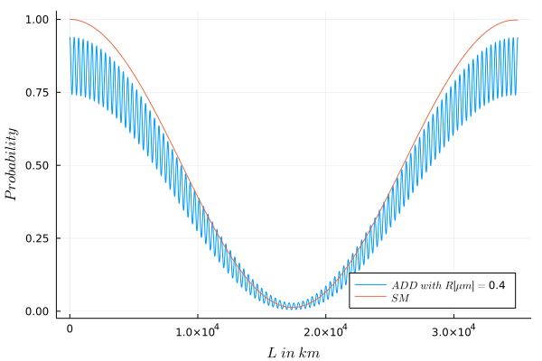
Figure 1: Survival probability of an electron neutrino in a three flavour ADD mixing scenario

Thus, the precision measurements of neutrino oscillations can put bounds on the critical value $\xi$ of the ADDM model.

Moreover, this deviation from the SM case also affects the unitarity of the Lepton Mixing Matrix. If the familiar three flavors of the SM neutrinos exhaust the spectrum of neutral leptons, the $3\times 3$ mixing matrix we measure in neutrino experiments must be unitary. This does not hold if there exist more than three neutrinos. In this case the Lepton Mixing Matrix is not a $3\times 3$ matrix anymore but a $(3+n)\times(3+n)$ matrix where $n$ is the number of additional neutrinos.

Nevertheless, in the experiments that are sensitive to active species, we would still measure only the $3\times 3$ part of the full Lepton Mixing Matrix. Since this restricted part in general will not be unitary, we will effectively register a deviation from unitarity. This happens also in the ADDM model where neutrinos can oscillate into the KK modes. Using the above results, the $3\times 3$ part of the full Lepton Mixing Matrix would get modified in the following way

$$\begin{pmatrix}U_{ee}\frac{1}{N_{e}}&U_{e\mu}\frac{1}{N_{e}}&U_{e\tau}\frac{1}{N_{e}}\\ U_{\mu e}\frac{1}{N_{\mu}}&U_{\mu\mu}\frac{1}{N_{\mu}}&U_{\mu\tau}\frac{1}{N_{\mu}}\\ U_{\tau e}\frac{1}{N_{\tau}}&U_{\tau\mu}\frac{1}{N_{\tau}}&U_{\tau\tau}\frac{1}{N_{\tau}}\\ \end{pmatrix}.$$ (125)

Now the task is to measure the parameters of the well known PMNS matrix very precisely and look for possible deviations from unitarity. Of course, this feature is not unique to ADDM and something similar can be realized in other models too. However, the above example provides us with concrete motivated framework for setting bounds on the unitarity-violating parameters and using them for discriminating between the different models. We are going to see this explicitly in the next section when we discuss phenomenology of the DR model and confront it with ADDM framework.

VI.2 Phenomenology of Dvali-Redi model

The generalisation of the mass matrix in the DR scenario goes as follows. Of course, the general structure of the mass matrix is again similar to (40) but this time the off-diagonal block matrices have the following form

$$M_{\alpha\beta}=\begin{pmatrix}m_{\alpha\beta}&0&0&\dots\\ 0&m_{\alpha\beta}&0&\dots\\ \vdots&0&\ddots&\vdots\end{pmatrix}.$$ (126)

This specific structure comes from the fact that in this theory the mixing among the different flavors can happen within a single copy since it is determined by the physics of the SM. This leads to the following electron neutrino eigenstate

$$\ket{\nu_{e}}=\sqrt{\frac{N-1}{N}}(U_{e1}\ket{m_{1}}+U_{e2}\ket{m_{2}}+U_{e3}\ket{m_{3}})+\frac{1}{\sqrt{N}}(U_{e1}\ket{m_{1}^{H}}+U_{e2}\ket{m_{2}^{H}}+U_{e3}\ket{m_{3}^{H}}).$$ (127)

The key parameter is the number of active species. Above we showed how we can group the total number of species into light and heavy sectors. Now one can investigate different scenarios with sectors which contain different numbers of copies. Because we have access predominantly to our copy of the SM, for us the scenarios with small number of active species in the sector our copy belongs to are of special interest. Due to this reason we focus on the scenarios with large heavy sectors that bring down the number of active species in our sector.

Taking the two expressions we found earlier for the Weinberg- and Dirac operator (83) and (107) and comparing them with each other, one sees that the oscillation into the other sector is suppressed by the number of the active species in the large sector. Therefore, one can safely ignore this contribution, especially in the Weinberg case since there it is further suppressed by the scale of the larger VEV $v^{\prime}$. Then the probability of survival in the one-flavour case Dvali and Redi (2009) is given by

$$P(t)=1-\frac{4}{N}\sin^{2}(\frac{\Delta m^{2}t}{2E}).$$ (128)

In this scenario, the problem of observing the effect is shifted from the large suppression by the amplitude into the extremely low frequency which comes from very small splitting among the mass eigenstates. Nevertheless, this case is still is of high potential interest for long-baseline experiments of neutrino oscillations. Astrophysical sources of high neutrino fluxes could be useful candidates for testing such scenarios. Of course, detection of deviations from the expected neutrino flux in pure SM requires understanding of the operation mechanisms of these sources to sufficiently high accuracy.

VI.2.1 Integrating out scenario

We observed that in small light sector scenarios the suppression of the amplitude goes contrary to the frequency of the oscillations. A scenario that can bring both parameters to the range of easier experimental accessibility is the “integrating out” scenario which we will now consider. The goal is to combine the advantages of the different above-studied scenarios into an unique setup. Let us assume that the permutation symmetry is broken very heavily among the two sectors: One sector containing a large number $M$ of copies and another sector containing a smaller number $N$. This is the case which we have already discussed above. However, let us now assume that due to additional breaking of the permutation symmetry, the smaller sector is further split into two sectors with the numbers $N^{\prime}$ and $M^{\prime}$. Obviously, the primary breaking of perturbation symmetry into the $M$ and $N$ sectors is still dominant and the secondary breaking does not affect physics up to effects of order $\mathcal{O}(\frac{N}{M})$ which is already negligibly small. Due to this reason, this sector can be considered as effectively decoupled from the other sectors.

Let us now turn our attention to the leftover copies that are broken down into two smaller sectors $N^{\prime}$ and $M^{\prime}$. Here we have a choice to which sector our SM copy belongs. In particular, we can assume that the number of copies in our sector $N^{\prime}$ is much larger than the other sector $M^{\prime}$. This does not decrease the suppression of the amplitude very much but allows us to liberate the value of the common heavy eigenstate $m_{H}$ in which the neutrinos of both sectors oscillate and can make $\Delta m$ large enough for bringing the frequency to a value comparable to the ordinary oscillations of the SM. This scenario of splitting is analogous to the large light sector scenario.

Overall this integrating out scenario enables us to free the both parameters of the theory. It allows us to bring down the number of copies and correspondingly oscillation frequencies to a scale that makes it observable for experiments.

We can now calculate the oscillation in the three-flavor case with an equal size splitting scenario. The equation for the survival probability can be written down as

$$P(\nu_{\mu}\rightarrow\nu_{\mu})=\sum_{i=1}^{6}\sum_{j=1}^{6}|U_{\mu i}|^{2}|U_{\mu j}|^{2}e^{\frac{i(m_{i}^{2}-m_{j}^{2})}{2E}}.$$ (129)

First we want to point out that in this expression no modes are averaged out like in the ADDM scenario. The reason for this is because just three additional mass eigenstates have to be included, meanwhile in ADDM scenarios the KK tower can inhabit a very large number of additional mass eigenstates. To analyze equation (129) further we split it up in the following way

$$P(\nu_{\mu}\rightarrow\nu_{\mu})=\left(\frac{N-1}{N}\right)^{2}\sum_{i=1}^{3}\sum_{j=1}^{3}|U_{\mu i}|^{2}|U_{\mu j}|^{2}e^{\frac{i(m_{i}^{2}-m_{j}^{2})}{2E}}+\frac{N-1}{N^{2}}\sum_{i=1}^{3}\sum_{j=4}^{6}|U_{\mu i}|^{2}|U_{\mu j}|^{2}e^{\frac{i(m_{i}^{2}-m_{j}^{2})}{2E}}\\ \\ +\frac{N-1}{N^{2}}\sum_{i=4}^{6}\sum_{j=1}^{3}|U_{\mu i}|^{2}|U_{\mu j}|^{2}e^{\frac{i(m_{i}^{2}-m_{j}^{2})}{2E}}+\frac{1}{N^{2}}\sum_{i=4}^{6}\sum_{j=4}^{6}|U_{\mu i}|^{2}|U_{\mu j}|^{2}e^{\frac{i(m_{i}^{2}-m_{j}^{2})}{2E}}.$$ (130)

The first term in this expression represents the oscillations within the flavors which are already known in the SM. For large $N$ these oscillations are just slightly modified. One also sees that the dominant contributions are coming from oscillations into the hidden species of order $\frac{1}{N}$ like in the one flavor case in equation (129). The contributions of solely the BSM terms are suppressed by $\frac{1}{N^{2}}$. Figure 2 shows the result of the calculations for a muon neutrino.

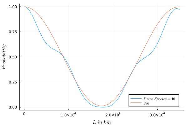
Figure 2: Survival probability of an muon neutrino in a three flavor case in DR model with an equal size splitting scenario

Let us also show the unitarity violation in the SM lepton mixing matrix which is expected by the DR scenario. For this we have to look into the formula (127). Picking out the $3\times 3$ block matrix in the upper left corner of the resulting mixing matrix we can write

$$\begin{pmatrix}\sqrt{\frac{N-1}{N}}U_{ee}&\sqrt{\frac{N-1}{N}}U_{e\mu}&\sqrt{\frac{N-1}{N}}U_{e\tau}\\ \sqrt{\frac{N-1}{N}}U_{\mu e}&\sqrt{\frac{N-1}{N}}U_{\mu\mu}&\sqrt{\frac{N-1}{N}}U_{\mu\tau}\\ \sqrt{\frac{N-1}{N}}U_{\tau e}&\sqrt{\frac{N-1}{N}}U_{\tau\mu}&\sqrt{\frac{N-1}{N}}U_{\tau\tau}\end{pmatrix}.$$ (131)

This is the matrix which is measured by experiments. One can immediately see that unitarity is violated by the overall factor of $\frac{N-1}{N}$. This is a characteristic signature of the theory and it comes from the democratic oscillation into the common heavy eigenstates of the neutrino matrix. The idea of testing the violation of unitarity experimentally by using availible experimental data is a still ongoing work Caldwell et al. .

VII Conclusions

In this paper we have focused on neutrino masses in the class of theories in which gravity cutoff is lowered down to $\sim$TeV scale. The two main frameworks accomplishing this lowering of the cutoff are ADD Arkani-Hamed et al. (1998, 1999) and “many species” Dvali (2010a); Dvali and Redi (2008) theories. In both cases, the decrease of the gravitational cutoff can be understood as a result of “dilution” of the graviton wave function in certain space labelled by a new coordinate. In both scenarios the volume of this space can be measured by the number of particle species. Correspondingly the role of the coordinate can be played by a species label. As shown in Dvali (2010a), in case of ADD Arkani-Hamed et al. (1998) the species represent the Kaluza-Klein excitations. Correspondingly, the extra space has an actual geometric meaning of large extra space dimensions. On the other hand, in “many species” solution to the hierarchy problem Dvali (2010a); Dvali and Redi (2008), the species can be arbitrary particles.

Previously it has been suggested that in both scenarios the small neutrino masses emerge naturally due to the dilution of the wave-function of the sterile (right-handed) neutrino in the extra space. Within ADDM this idea was introduced in Arkani-Hamed et al. (2001) and its phenomenological implications were studied in Dvali and Smirnov (1999). In this case the wave-function of the sterile neutrino is diluted in the actual geometric extra space. This results into a highly suppressed Yukawa coupling between the sterile and the active neutrino of the SM, thereby, generating a tiny neutrino mass. As shown in Dvali and Smirnov (1999) due to the mixing of active left-handed neutrino with the KK tower of the sterile partner, a non-trivial oscillation pattern emerges.

More recently, it has been shown Dvali and Redi (2009) that a similar suppression mechanism of the neutrino mass works in the DR scenario Dvali (2010a); Dvali and Redi (2008) in which species represented the identical copies of the SM and the role of the extra coordinate is played by their label. Using this framework, it was shown in Dvali and Redi (2009) that the dilution of the wave-function of the sterile neutrino in the space of species results into a small neutrino mass. However, as discussed there the phenomenological aspects of this scenario are very different from the case of Arkani-Hamed et al. (2001) which relies on ADDM framework.

In this paper, we have generalized the above original proposals in certain directions. In particular, we included a more realistic case of three SM neutrino flavors. We adopted the universal language of species which allows to capture some general aspects of the neutrino mixing matrix and confront different scenarios.

We calculated an approximate formula for the flavor eigenstates of a general mass matrix using perturbation theory in the three flavor case. Next, we showed how highly symmetric mass matrices can be calculated in an exact manner and we investigated different symmetry breaking patterns of these highly symmetric mass matrices. We gave the explicit expressions for flavor eigenstates for each case.

Our further step was to apply this generally derived formulas to the explicit theories of neutrino masses such as the proposal of ADDM Arkani-Hamed et al. (2001); Dvali and Smirnov (1999) within ADD and the one of DR Dvali and Redi (2009) within Many Species frameworks respectively. Here we used the derived formulas and gave a three flavour solution that depends on the parameters of the specific theories.

As it was already pointed out in Dvali and Smirnov (1999) and Dvali and Redi (2009) within ADDM and DR frameworks, the generic prediction of both scenarios is the non-conservation of neutrino number within SM. This is due to the mixing of SM active neutrinos with the tower of sterile partners. This mixing results into the oscillations of neutrinos into hidden species as well as in seeming violation of unitarity within the SM lepton sector.

Correspondingly, our calculations of these effects for three-flavor case have important phenomenological implications in both directions. First is the account of deviations of neutrino oscillations from the case of SM. Second, is the parameterization of violation of unitarity of the PMNS-Matrix.

The structures unitarity-violation in the two different theories (ADDM Arkani-Hamed et al. (2001); Dvali and Smirnov (1999) of ADD versus Dvali-Redi Dvali and Redi (2009) of Many Species) differ from each other. Our analyses therefore has a discriminating power between these two theories.

In general, we can say that small neutrino mass generation via mixing with large number of extra species is an exciting field with different phenomenological effects on the low energy neutrino physics. These effects can be searched for both in current neutrino experiments, such as IceCube Ahlers et al. (2018), as well as in the planned ones like JUNO et al. (2016). Here, the violation of unitarity can be tested and one can use their results to give bounds on the parameters of the theories such as the size of the extra dimensions in ADDM or the number of sterile neutrino species to which our neutrino mixes within many species scenario.

References

- Dvali (2017) G. Dvali, Subnucl. Ser. 53, 189 (2017), arXiv:1607.07422 [hep-th] .
- Arkani-Hamed et al. (1998) N. Arkani-Hamed, S. Dimopoulos, and G. R. Dvali, Phys. Lett. B 429, 263 (1998), arXiv:hep-ph/9803315 .
- Arkani-Hamed et al. (1999) N. Arkani-Hamed, S. Dimopoulos, and G. R. Dvali, Phys. Rev. D 59, 086004 (1999), arXiv:hep-ph/9807344 .
- Antoniadis et al. (1998) I. Antoniadis, N. Arkani-Hamed, S. Dimopoulos, and G. Dvali, Phys. Lett. B 436, 257 (1998), arXiv:hep-ph/9804398 .
- Dvali (2010a) G. Dvali, Fortsch. Phys. 58, 528 (2010a), arXiv:0706.2050 [hep-th] .
- Dvali and Redi (2008) G. Dvali and M. Redi, Phys. Rev. D 77, 045027 (2008), arXiv:0710.4344 [hep-th] .
- Dvali (2010b) G. Dvali, Int. J. Mod. Phys. A 25, 602 (2010b), arXiv:0806.3801 [hep-th] .
- Dvali and Gomez (2009) G. Dvali and C. Gomez, Phys. Lett. B 674, 303 (2009), arXiv:0812.1940 [hep-th] .
- Dvali and Redi (2009) G. Dvali and M. Redi, Phys. Rev. D 80, 055001 (2009), arXiv:0905.1709 [hep-ph] .
- Dvali and Gomez (2010) G. Dvali and C. Gomez, (2010), arXiv:1004.3744 [hep-th] .
- Dvali (2021) G. Dvali, (2021), arXiv:2103.15668 [hep-th] .
- Arkani-Hamed et al. (2001) N. Arkani-Hamed, S. Dimopoulos, G. R. Dvali, and J. March-Russell, Phys. Rev. D 65, 024032 (2001), arXiv:hep-ph/9811448 .
- Dvali and Smirnov (1999) G. R. Dvali and A. Y. Smirnov, Nucl. Phys. B 563, 63 (1999), arXiv:hep-ph/9904211 .
- Fantini et al. (2018) G. Fantini, A. G. Rosso, F. Vissani, and V. Zema, (2018), doi:10.1142/97898132260980002, arXiv:1802.05781 [hep-ph] .
- Aker et al. (2019) M. Aker, K. Altenmüller, M. Arenz, M. Babutzka, J. Barrett, S. Bauer, M. Beck, A. Beglarian, J. Behrens, T. Bergmann, and et al., Physical Review Letters 123 (2019), 10.1103/physrevlett.123.221802, arXiv:1909.06048v1 [hep-ex].
- Weinberg (1979) S. Weinberg, Phys. Rev. Lett. 43, 1566 (1979).
- Minkowski (1977) P. Minkowski, Phys. Lett. B 67, 421 (1977).
- Gell-Mann et al. (1979) M. Gell-Mann, P. Ramond, and R. Slansky, Conf. Proc. C 790927, 315 (1979), arXiv:1306.4669 [hep-th] .
- Yanagida (1980) T. Yanagida, Prog. Theor. Phys. 64, 1103 (1980).
- Mohapatra and Senjanovic (1980) R. N. Mohapatra and G. Senjanovic, Phys. Rev. Lett. 44, 912 (1980), doi:10.1103/PhysRevLett.44.912.
- Mohapatra (2004) R. Mohapatra, SEESAW25: International Conference on the Seesaw Mechanism and the Neutrino Mass, , 29 (2004), arXiv:hep-ph/0412379v1, arXiv:hep-ph/0412379, doi:10.1142/9789812702210-0003 .
- Dvali et al. (2009) G. Dvali, I. Sawicki, and A. Vikman, Journal of Cosmology and Astroparticle Physics 2009, 009–009 (2009), arXiv:0903.0660v1 [hep-th], doi:10.1088/1475-7516/2009/08/009.
- (23) A. Caldwell, G. Dvali, P. Eller, and M. Ettengruber, ongoing work .
- Dvali and Shifman (1997) G. R. Dvali and M. A. Shifman, Phys. Lett. B 396, 64 (1997), [Erratum: Phys.Lett.B 407, 452 (1997)], arXiv:hep-th/9612128 .
- Esteban et al. (2020) I. Esteban, M. Gonzalez-Garcia, M. Maltoni, T. Schwetz, and A. Zhou, Journal of High Energy Physics 2020 (2020), 10.1007/jhep09(2020)178.
- Ahlers et al. (2018) M. Ahlers, K. Helbing, and C. Pérez de los Heros, The European Physical Journal C 78, 924 (2018), arXiv:1806.05696v1 [astro-ph.HE], doi: 10.1140/epjc/s10052-018-6369-9.
- et al. (2016) F. A. et al., Journal of Physics G: Nuclear and Particle Physics 43, 030401 (2016), arXiv:1507.05613v2 [physics.ins-det], doi:10.1088/0954-3899/43/3/030401.