A new mixed-integer programming model for irregular strip packing based on vertical slices with a reproducible survey

Abstract

The irregular strip-packing problem, also known as nesting or marker making, is defined as the automatic computation of a non-overlapping placement of a set of non-convex polygons onto a rectangular strip of fixed width and unbounded length, such that the strip length is minimized. Nesting methods based on heuristics are a mature technology, and currently, the only practical solution to this problem. However, recent performance gains of the Mixed-Integer Programming (MIP) solvers, together with the known limitations of the heuristics methods, have encouraged the exploration of exact optimization models for nesting during the last decade. Despite the research effort, the current family of exact MIP models for nesting cannot efficiently solve both large problem instances and instances containing polygons with complex geometries. In order to improve the efficiency of the current MIP models, this work introduces a new family of continuous MIP models based on a novel formulation of the NoFit-Polygon Covering Model (NFP-CM), called NFP-CM based on Vertical Slices (NFP-CM-VS). Our new family of MIP models is based on a new convex decomposition of the feasible space of relative placements between pieces into vertical slices, together with a new family of valid inequalities, symmetry breakings, and variable eliminations derived from the former convex decomposition. Our experiments show that our new NFP-CM-VS models outperform the current state-of-the-art MIP models. Finally, we provide a detailed reproducibility protocol and dataset based on our Java software library as supplementary material to allow the exact replication of our models, experiments, and results.

1 Introduction

Cutting and packing regular (convex) and irregular (non-convex) polygons onto a rectangular strip with unbounded length is a tedious and omnipresent task in most manufacturing industries based on the cutting of any flat material. For instance, Milenkovic et al. [58] study the nesting problem for the fashion and apparel industry, whilst Heistermann and Lengauer [45] and Whelan and Batchelor [95] do it on leather manufacturing, Elamvazuthi et al. [36] in furniture, Han et al. [44] in the glass industry, Alves et al. [8] in the automotive industry, and Cheok and Nee [18] in shipbuilding. The irregular strip-packing methods aim to compute a non-overlapping placement of a set of irregular polygons onto a fixed-width rectangular strip with unbounded length, called the board, whose length is the minimum between all feasible placements. Another closely related problem, called two-dimensional bin packing [57], is defined as the computation of a non-overlapping placement of a set of polygons onto a larger closed polygon, called the bin, to minimize the number of bins required. Although most of bin packing problems are defined for rectangular bins and items [47], we also find many irregular bin packing problems in the aforementioned industries. Strip and bin packing problems, and all their variants concerning the geometry of the pieces or boards, belong to the broader family of Cutting and Packing (C&P) problems categorized by Dyckhoff [35] and Wäscher et al. [94], and extensively reviewed by Sweeney and Paternoster [90], Dowsland and Dowsland [32], Wang and Wäscher [93], and Bennell et al. [14].

Research on the irregular strip and bin packing problems can be traced back to the pioneering Linear Programming (LP) models for rectangular bin packing introduced by Gilmore and Gomory [41], and the pioneering heuristic methods for irregular strip packing proposed by Art [11], Adamowicz and Albano [2, 1], and Albano and Sapuppo [5] in the late nineteen sixties and seventies. These early works introduce many of the basic ideas subsequently exploited by all heuristics methods reported in the literature, such as the notion of a feasible non-overlapping region between pieces based on the No-Fit Polygon (NFP) representation, and the sequential placement of pieces based on a bottom-left heuristics. Given two polygons $A,B\subset\mathbb{R}^{2}$, the no-fit polygon of $B$ regarding $A$ is defined by $NFP_{AB}=A\oplus(-B(0,0))$, where $\oplus$ symbol denotes the Minkowski sum of two sets $S_{1},S_{2}\subset\mathbb{R}^{2}$, such that $S_{1}\oplus S_{2}=\{p+q:p\in S_{1},q\in S_{2}\}$ and $B(0,0)$ is the translation of the polygon $B$ such that its reference point is positioned at the origin. The boundary and outer region of the no-fit polygon $NFP_{AB}$ set the feasible positions in which polygon $B$ can be placed without rotating into a non-overlapping position regarding polygon $A$. The no-fit polygon allows computing the feasible relative placements for any polygon pair $(A,B)$ a priori by checking whether their relative position vector $(x_{B}-x_{A},y_{B}-y_{A})$ belongs to either the boundary or the outer region of $NFP_{AB}$. Consequently, this later property has converted the NFP into the most broadly adopted and effective geometric representation for the nesting problem reported in the literature, both by the families of heuristics methods [13] and exact mathematical models [53].

Fowler et al. [40] and Milenkovic et al. [58] show that the irregular strip-packing problem is NP-complete. For this reason, most practical solutions reported in the literature since the pioneering work of Art [11] are based on sequential placement heuristics to build efficiently feasible solutions that are combined with meta-heuristics for exploring the space of feasible solutions, as shown in most of surveys on nesting [33, 34, 46, 13, 70]. Current heuristics-based methods can efficiently compute acceptable solutions for large problem instances, which have encouraged their early and extensive adoption in all industries mentioned above, especially in those industries with a so significant and permanent diversity of products as the garment industry [66]. Elkeran [37] introduces the current state-of-the-art heuristics method for nesting, called Guided Cuckoo Search (GCS), which defines a two-stages method based on piece clustering and a NFP-based bottom-left heuristics [42] to build an initial feasible solution that is shrinked by solving an overlap minimization problem using a variant of the cuckoo search meta-heuristics. Although GCS was introduced almost a decade ago, subsequent works have been unable to outperform its results, as shown by Pinheiro et al. [65, table 3], Sato et al. [78, table 5], Cherri et al. [22, table 4], Mundim et al. [62, table 6], Amaro Júnior et al. [9, table 2], and Sato et al. [77, tables 4-5]. GCS [37] also significantly outperforms a commercial nesting system broadly adopted in the industry [10, figure 3]. However, the heuristics methods demand several hours to improve their initial solutions [62, table 6], and they can neither provide an optimality proof nor a gap measure to the optimal solution.

Recent performance gains of the Mixed-Integer Programming (MIP) solvers, and the limitations of the heuristics methods mentioned above, have encouraged the exploration of exact mathematical models for nesting during the last decade, as shown by Leao et al. [53]. The mathematical models for nesting can be categorized into continuous, discrete, or semi-continuous models according to the type of decision variable used to represent the position of the pieces. Li [54, §8] introduces the first continuous MIP model for nesting reported in the literature to solve a limitation of the pioneering LP compaction model of Li and Milenkovic [55, 56]. Despite Li’s model is not experimentally evaluated, it sets the two main features of the family of continuous MIP models based on the NFP as follows: (1) the convex decomposition of the outer NFP feasible regions; and (2) the definition of mutually-exclusive binary variables to set the pairwise non-overlapping constraints between pieces defining the feasible regions for their relative placement. Thus, we say that Li’s model sets the basic continuous linear MIP model for nesting without rotations, from which all subsequent works, including the present work, introduce more tightened and refined formulations. For instance, Dean [30, §5] introduces and evaluates for the first time a MIP model for nesting based on a refinement of the Daniels et al. [29] bin packing model that is essentially identical to the Li’s model. Subsequently, Fischetti and Luzzi [39] (F&L) introduce a refinement of Li’s model based on lifting the big-M formulation and a branching-priority algorithm to guide the Branch&Bound (B&B) exploration by fixing large sets of feasible relative placements among pieces. Álvarez-Valdés et al. [7] improve the F&L model by introducing a new MIP model called HS2, which is based on a detailed convex decomposition of the feasible regions, a lifting for the bound constraints of the continuous variables, six new branching strategies, and the x-axis ordering of identical pieces to remove all symmetric solutions derived from their permutation. However, the HS2 model [7] cannot significantly improve the F&L model despite all their improvements.

More recently, Cherri et al. [25] introduce two continuous MIP models improving the HS2 model [7], together with the first MIP model integrating discrete rotations, which are based on the convex decomposition of the pieces and the definition of the non-overlapping constraints between pieces by using the convex no-fit polygons among their convex parts. The first model, called Direct Trigonometry Mode (DTM), uses a direct trigonometry function encoding the separation lines defined by the edges of the polygons to build the non-overlapping constraints between pairs of convex parts from two pieces, whilst the second model, called NoFit-Polygon Covering Model (NFP-CM), uses the convex NFP between convex parts and several valid inequalities. DTM and NFP-CM use the same x-axis symmetry-breaking for identical pieces proposed by Alvarez-Valdes et al. [6]. Subsequently, Rodrigues et al. [73] improve the NFP-CM model by breaking the symmetries of the feasible space for the relative placements between pieces, setting the current state-of-the-art in terms of performance among the family of exact continuous mathematical models for irregular strip packing. However, the Improved NFP-CM model [73] is only able to solve small problem instances with up to 17 pieces with simple geometry [73, table 2], and unlike the NFP-CM model [25, table 3], it has not been evaluated on complex small and large problem instances yet.

The main aim of this work is to introduce a new family of continuous MIP models for irregular strip packing without rotations capable of improving the performance of current state-of-the-art MIP models. The new family of MIP models, called NFP-CM based on Vertical Slices (NFP-CM-VS), is a novel and more tightened formulation of the state-of-the-art NFP-CM models [25, 73] that is based on a new disjoint convex decomposition of the feasible regions between convex parts into vertical slices, together with a new family of valid inequalities, symmetry breakings, and variable reductions derived from the former geometric decomposition. A second aim of this work is to carry out a fair reproducible comparison of our new family of MIP models with the state-of-the-art family of NFP-CM models [25, 73] by replicating these later models and implementing our new MIP models into a single software platform integrating the latest version of the Gurobi solver, which will be provided together with a detailed reproducibility protocol and dataset as supplementary material to allow the exact replication of all our models, experiments, and results.

1.1 Motivation and hypothesis

Our main motivation is the proposal and evaluation of a new and more tightened formulation of the family of NFP-CM models introduced by Cherri et al. [25] and Rodrigues et al. [73]. Our main hypothesis is that the new NFP-CM-VS models could improve the performance of the current state-of-the-art MIP models.

The second motivation of this work is to implement a reproducible experimental survey for a fair and confirmatory comparison of all models, which is based on our software implementation of all MIP models evaluated herein into a single Java software library based on the latest version of the Gurobi solver, called Gurobi 9.5.

A third motivation is to bridge the lack of reproducibility resources hampering the independent replication and confirmation of previously reported models and results, as well as the incorporation of newcomers into this area, by providing a detailed reproducibility protocol and dataset as supplementary material to allow the exact replication of all MIP models evaluated herein, as well as all our experiments and results.

And finally, our fourth motivation is a confirming evaluation for the first time of the state-of-the-art Improved NFP-CM model [73] in the same problem instances reported for NFP-CM [25, tables 1-2] to provide a fair and updated benchmark of the current state-of-the-art MIP models for nesting. We also evaluate the NFP-CMnc model [25] in a set of large problem instances not reported before.

1.2 Definition of the problem and contributions

The irregular strip-packing problem can be abstractly defined regardless of the geometric representation of the non-overlapping constraints as follows. Let be $\mathcal{P}=\{P_{i}\}_{i=1,\dots,n}$ the set of pieces to be placed onto the board $\mathcal{B}$, $T=\{t_{i}\}_{i=1,\dots,n}$ and $R=\{r_{i}\}_{i=1,\dots,n}$ the set of translation vectors and orientations defining a feasible solution of the problem, $L$ the length of the board, $\mathcal{O}$ the set of admissible orientations, $P(r)\subset\mathbb{R}^{2}$ denotes an orientation of the piece $P$, and $int(A)$ denotes the interior set for any set $A\subset\mathbb{R}^{2}$ with the usual topology of $\mathbb{R}^{2}$. Then, the minimization problem (1) defines the optimal solution to the irregular strip packing problem, where constraints (2) prevent the overlapping of pieces, and constraints (3) force the pieces to be entirely contained in the board.

minimize $$L$$ (1)

subject to $$int(P_{i}(r_{i})\oplus t_{i})\cap int(P_{j}(r_{j})\oplus t_{j})=\varnothing,\quad 1\leq i<j\leq n$$ (2)

$$(P_{i}(r_{i})\oplus t_{i})\subseteq\mathcal{B},\quad 1\leq i\leq n$$ (3)

$$t_{i}\in\mathbb{R}^{2},r_{i}\in\mathcal{O},L\in\mathbb{R}_{>0}$$ (4)

The main research problem tackled in this work is the definition and evaluation of a new and more tightened MIP model for irregular strip packing than the current state-of-the-art family of NFP-CM models [25, 73]. Our main contribution is the introduction of a new family of MIP models, called NFP-CM-VS, which is based on a new convex decomposition of the feasible regions between convex parts into vertical slices, together with a new family of valid inequalities, symmetry breakings, and variable eliminations derived from the former geometric decomposition. Our second significant contribution is the introduction of the first reproducible experimental survey in this line of research, which is based on our software implementation of all models evaluated herein into a Java software library, together with a detailed reproducibility protocol and dataset to allow the exact replication of all our models and results.

The rest of the paper is structured as follows. Section 2 reviews the literature on exact mathematical models for irregular strip packing. Section 3 introduces our new family of MIP models, whilst the section 4 details our experimental setup and results, and section 5 introduces our discussion of the results. Next section summarizes our main conclusions and future work. Subsequently, Appendix A introduces all raw output data generated for each MIP model evaluated herein not included in the results section because of lack of room. Finally, Appendix B introduces a detailed reproducibility protocol based on our supplementary dataset [50] to allow the exact replication of all our models, experiments, and results. Both aforementioned appendices are provided as supplementary material.

2 Related work on exact models for nesting

Our introduction has provided a detailed review of the family of continuous MIP models for irregular strip packing based on the NFP, to which this work belongs. In addition, this section introduces a comprehensive categorization of the literature on exact mathematical models for nesting, together with an extended review of the linear MIP models based on the NFP. However, for a detailed and recent review of the family of mathematical models, we refer the reader to the survey of Leao et al. [53] and the survey on geometric representations for nesting of Bennell and Oliveira [12] .

Exact models

for

irregular

strip packing - Linear

MIP

models - based on

the NFP - Continuous

positions - Li [54], Dean [30], Fischetti and Luzzi [39]

- Alvarez-Valdes et al. [6, HS1, HS2]

- Cherri et al. [25, NFP-CM]

- Rodrigues et al. [73]

- Santoro and Lemos [76, special convex pieces]

- Family of NFM-CM-VS models (ths work)

- Discrete

positions - Toledo et al. [91, Dotted-Board (DB)]

- Rodrigues and Toledo [74, Clique covering + DB]

- Cherri et al. [23, DB with discrete rotations]

- Al Theeb et al. [4, Improved DB Model (IDBM)]

- Rodrigues&Andretta [81, 82, Stochastic DB])

- Semi-continuous positions - Leao et al. [52, y-axis discretization], - Leao and Toledo [51]
- based on Direct Trigonometry (DT) - Cherri et al. [25, DTM] - Cherri et al. [25, DTM + discrete rotations]
- Non-Linear Programming (NLP) models (continuous rotations) - based on $\Phi$-functions - Stoyan et al. [88, 89], Stoyan and Romanova [86], - Chernov et al. [19, 20], - Stoyan et al. [87, 83, 84, 85] - Pankratov et al. [63], Romanova et al. [75] - based on circle coverings - Jones [48], Rocha et al. [72] - Rocha et al. [71], Wang et al. [92] - based on Direct Trigonometry and the NFP - Kallrath [49, non-convex NLP&MINLP models]     (restricted to circles, rectangles, and convex pieces) - Cherri et al. [24, convex MIQCP model] - Peralta et al. [64, non-convex NLP model]
- Constraint Programming (CP) models based on the NFP - Ribeiro et al. [69, convex pieces] - Carravilla et al. [17, irregular pieces] - Ribeiro and Carravilla [67, 68, global nesting constraint] - Carravilla and Ribeiro [16, hybrid CP-MIP] - Cherri et al. [21, new global constraint + DB model]

Figure 1: Categorization of exact mathematical models for irregular strip packing.

2.1 Categorization of exact mathematical models

Figure 2 shows our categorization of the family of exact continuous mathematical models for irregular strip packing reported in the literature, which can be divided into three large families as follows. First, the family of Linear MIP models based on the NFP, whose main features are the convex decomposition of the feasible regions defined by the pairwise NFP between pieces and the use of mutually exclusive binary variables to select their relative placements, such as the family of continuous models pioneered by Li [54, §8], Dean [30, §5], and Fischetti and Luzzi [39], which are subsequently refined by Alvarez-Valdes et al. [6], Cherri et al. [25], and Rodrigues et al. [73]. Second, the family of Constraint Programming (CP) models based on the NFP, whose pioneering work is introduced by Ribeiro et al. [69], and subsequently improved by Carravilla et al. [17], Ribeiro and Carravilla [68], and Cherri et al. [21]. And third, Other models based on alternatives geometric representations and Non-Linear Programming (NLP) models, such as (3.a) the family of models based on $\Phi$-functions, whose pioneering works are introduced by Stoyan et al. [88], Chernov et al. [19], and Stoyan et al. [89]; (3.b) others non-linear models based on direct trigonometry introduced by Rocha et al. [71], Cherri et al. [24], and Peralta et al. [64]; and finally, (3.c) the family of models based on circle coverings admitting free rotations, whose pioneering work is introduced by Jones [48] and subsequently refined by Rocha et al. [72], Rocha et al. [71], and Wang et al. [92].

Likewise, the linear MIP models can be divided into three subfamilies according to the nature of the decision variables encoding the $(x,y)$ position of the pieces as follows: (1) continuous models, such as the former aforementioned ones [54, 30, 39, 6, 25, 73]; (2) discrete models like the pioneering Dotted-Board model of Toledo et al. [91], subsequently refined by Rodrigues and Toledo [74]; and (3) semi-continuous models as that proposed by Leao et al. [52]. On the other hand, the linear MIP models can also be divided into models based on the NFP or direct trigonometry according to the geometric representation used for building the non-overlapping constraints, as shown in figure 2.

2.2 Linear continuous MIP models

We summarize the review of linear continuous MIP models advanced in our introduction as follows. Li [54, §8] introduces the first continuous MIP model for irregular strip packing reported in the literature, whilst Dean [30, §5] evaluates for the first time a minor adaptation of the Li’s model, and Fischetti and Luzzi [39] introduce and experimentally evaluate a refinement of the Li’s model based on a lifting of the big-M formulation together with a branching-priority algorithm, which is subsequently refined by Álvarez-Valdés et al. [7] by introducing the HS2 model based on a detailed convex decomposition of the feasible space of relative placements between pieces, a lifting for the bound constraints of the continuous variables, and six new branching strategies. More recently, Cherri et al. [25] introduce two continuous MIP models, called DTM and NFP-CM, which are based on the convex decomposition of the pieces and the definition of the non-overlapping constraints between pieces by using either direct trigonometry or the convex no-fit polygons among their convex parts, together with some valid inequalities and a variable elimination. Subsequently, Rodrigues et al. [73] improve the NFP-CM model by breaking the symmetries in the feasible space of relative placements between pieces. On the other hand, Santoro and Lemos [76] introduce an exact MIP model to compute efficiently tighter upper bounds for the irregular nesting problem based on approximating the input pieces by parallel-chamfered n-gons with up to 8 sides, as shown in Santoro and Lemos [76, fig. 2], and generalizing the disjunctive MIP model for rectangular strip packing proposed by Sawaya and Grossmann [80].

Figure 2: Disjoint convex decomposition of the feasible relative placements between pieces defined by each model in the family of continuous MIP models for irregular strip packing. Each single convex feasible sub-region in figures (a)-(d) above is enabled by a mutually-exclusive binary variable $v_{ij}^{k}$. The Fischetti and Luzzi (a) and HS2 (b) models set their non-overlapping constraints using the overall no-fit polygon $NFP_{ij}$ between pieces $i$ and $j$, whilst the NFP-CP models (c-d) set them using the convex NFP parts between each pair of convex parts of two pieces. Figure (c) shows in green the space of symmetric solutions generated by adjacent feasible sub-regions of the NFP-CM model [25], whilst figure (d) shows the symmetry-breaking of the former model proposed by the Improved NFP-CM model [73].

Regardless of the minor differences in the formulation of the continuous MIP models mentioned above, their main difference is the geometric decomposition of the feasible space of relative placements between pieces used to build the non-overlapping constraints, as shown in figure 2. Fischetti and Luzzi [39] propose a convex decomposition of the feasible regions using the overall $NFP_{ij}$ between pieces $i$ and $j$, as shown in figure 2.a. However, Fischetti and Luzzi do not provide a detailed definition of its geometry, which encourages Alvarez-Valdes et al. [6] to propose a well-defined convex decomposition based on horizontal slices to build their HS2 model, as shown in figure 2.b. Subsequently, Cherri et al. [25] propose a convex decomposition of the pieces and the definition of their non-overlapping constraints by using the convex no-fit polygons among their convex parts, as shown in figure 2.c. The convex decomposition proposed by Cherri et al. for their NFP-CM model provides two key advantages on previous MIP models as follows: (1) it avoids the need to explicitly compute the overall NFP between irregular pieces by computing the NFP between convex parts, which is much easier than the former; and, (2) it allows building the non-overlapping constraints between pieces using only one constraint per binary variable, unlike the previous MIP models that require at least three constraints per binary variable. However, one significant drawback of the NFP-CM model [25] is the existence of symmetric solutions induced by the overlapping of adjacent feasible sub-regions, as shown by regions in green in figure 2.c, which encourages Rodrigues et al. [73] to break these symmetries by inserting one additional constraint per binary variable activating a separation line defined by the previous edge in the polygon’s boundary, as shown in figure 2.d, at the cost of doubling the number of non-overlapping constraints to break the symmetries in their geometric decomposition.

The main limitation of the family of current continuous MIP models based on the NFP approach is their inability to solve either large problem instances or instances including pieces with complex geometries, which we attribute to two difficulties derived from their structure as follows: (1) the large number of binary variables needed to build the non-overlapping constraints between pieces; and (2) a poor tightening of the LP relaxed model as a consequence of encoding the linearization of a min-max model in the objective function that does not directly depend on the binary variables. For instance, the number of binary variables in current continuous exact MIP models [39, 6, 25, 73] is quadratic regarding the number of pieces $n$ with scalability factor $\mathcal{O}(r^{4}\frac{n}{2}(n-1))$, whilst the number of non-overlapping constraints might be up to three times the latter factor, where $r$ is the average number of edges per piece. The $\frac{1}{2}n(n-1)$ factor is derived from the pairwise combinatory nature of the problem, whilst the $r^{4}$ gives account of the geometric complexity of the pieces, which derives from the fact that the resulting NFP from two polygons with $s$ and $t$ edges might has $O(s^{2}t^{2})$ edges in the worst case [3, p.40], although it is at most $s+t$ for convex polygons. Thus, the complexity of current continuous MIP models grows rapidly regarding both the number of pieces and its geometric complexity.

2.3 Discrete and semi-continuous MIP models

For the reasons detailed above, several authors have proposed discrete MIP models to solve efficiently large problem instances as follows: (1) the discrete models based on a grid representation of the board introduced by Toledo et al. [91], which is refined by Rodrigues and Toledo [74] using a clique-based formulation, being subsequently extended by Rodrigues de Souza and Andretta [81, 82] to deal with the uncertainty in the demand of the pieces using a two-stage stochastic programming model; and finally, (2) the semi-continuous model based on the discretization of the y-axis introduced by Leao et al. [52]. The Dotted-Board model (DB) model of Toledo et al. [91] is able to solve problem instances with up to 56 pieces of two types to optimality (see [91, table 3]), whilst the semi-continuous MIP model of Leao et al. [52] removes the resolution error in the x-axis direction and allows solving instances with up to 70 pieces and larger boards [52, table 1] than the DB model. However, the discrete models above are approximations of the exact continuous problem. Thus, the quality of their solutions depends on the grid resolution, as shown experimentally by Sato et al. [79]. Moreover, the computational cost of the discrete models also grows rapidly with the resolution of the grid and the number of different piece types, which encouraged several improvements to the DB model as follows. Rodrigues and Toledo [74] propose a new clique-based formulation of the DB model, whilst Cherri et al. [23] propose two methods to build non-regular grids together with an efficient data structure to represent them. The grid representation, also called no-fit raster, is also used by recent state-of-the-art heuristics methods [62, 61].

3 The new family of MIP models for nesting

This section introduces two new MIP models for irregular strip packing based on a new disjoint convex decomposition of the space of feasible placements between pieces defined by the pairwise convex NFP between their convex parts, together with a set of valid inequalities, symmetry breakings, and variable eliminations derived from the former decomposition. The use of the convex NFP between convex parts of the pieces to build the pairwise non-overlapping constraints is the core innovation of the family of NFP-CM models proposed by Cherri et al. [25] and subsequently improved by Rodrigues et al. [73] to break the symmetries of the NFP-CM model, as shown in figure 2.d. Thus, our new MIP models set a more tightened formulation than the NFP-CM model for the same feasible space of relative placements between pieces by defining a new set of constraints and two new binary variables based on our new disjoint convex decomposition shown in figure 3.1. Our new NFP-CM-VS models include at most 2 binary variables more per convex NFP part than the NFP-CM model [25] to encode the left and right feasible sub-regions shown in figure 3.1 in those cases in which the NFP’s boundary does not include a vertical edge in some of their sides.

The two aims of our new convex decomposition are as follows: (1) to break the symmetries of the feasible solutions; and (2) to infer a large number of unfeasible relative placements among three pieces or two pieces of the same type, which can be hand-coded either as feasibility cuts or by removing some binary variables from the model, respectively. Our new feasibility cuts among three pieces can also be generalized to combinations of more than three pieces; however, we limit our evaluation herein to piece triplets. First, we introduce the basic formulation of our new MIP model called No-Fit Polygon Covering Model based on Vertical Slices (NFP-CM-VS). Next, we introduce several families of valid inequalities and variable eliminations to break the symmetries and remove some unfeasible solutions derived from the convex NFP parts between two pieces, as well as a family of feasibility cuts among three pieces. Finally, we introduce the NFP-CM-VS2 model integrating all cuts and variable eliminations of the full NFP-CM-VS model but removes the big-M terms for the constraints encoding the vertical slices of our convex decomposition by factorizing all x-axis constraints into two single constraints per convex NFP part.

3.1 Basic notation and geometric tools

Representation of the pieces. Figure 3 details the meaning of the parameters used to represent the geometry of the pieces and the board. The board is represented by an open rectangle of fixed height $H$ and variable length $L$, whose lower and upper bounds are denoted by $L_{lb}$ and $L_{ub}$ respectively. We use a standard orthogonal x-y reference frame setting the origin of the board in its bottom-leftmost corner. Each piece $P_{i}$ is defined by an irregular polygon decomposed into a set of disjoint convex polygons, called convex parts, whose boundaries are represented by a counter-clockwise ordered list of points in the plane, called vertices, such that each pair of consecutive vertices defines a line segment, called edge. We use the indexes $f$ and $g$ to denote the source convex parts generating the convex $NFP_{ij}^{fg}$ part between the pieces $P_{i}$ and $P_{j}$. For each piece $P_{i}$, one arbitrary vertex from any of its convex parts is selected as reference point, denoted by $r_{i}=(x_{i},y_{i})$, to set the continuous decision variables representing the position of the piece $i$ on the board. The parameters $l_{i}^{min}$ and $l_{i}^{max}$ denote the x-axis distance from the leftmost and rightmost points of piece $i$ to its reference point $r_{i}$, respectively, whilst $h_{i}^{min}$ and $h_{i}^{max}$ denote the y-axis distance from the topmost and bottommost points of piece $i$ to $r_{i}$. The type of each piece $i$ is denoted by $t_{i}$, whilst their area and demand are denoted by $\Delta_{t}$ and $d_{t}$ respectively.

Convex decomposition of pieces. To build the non-overlapping constraints of our family of NFP-CM-VS models, all non-convex pieces must be decomposed into convex polygons, as shown in figure 3. Thus, each piece $P_{i}$ is defined as the union of $Q_{i}$ convex parts as follows $P_{i}=\bigcup\limits_{f=1}^{Q_{i}}P_{i}^{f}$. We use the Green’s convex decomposition algorithm [43] implemented by the CGAL library to decompose the pieces into convex parts as proposed by Cherri et al. [25], with the aim of replicating their NFP-CM models and experiments. The Greene’s algorithm efficiently approximates the optimal convex decomposition of a polygon without adding new vertices to its boundary. However, there are many other alternatives in the literature [38] that could potentially generate fewer number of edges, and thus fewer binary variables, than the Greene’s algorithm. For instance, we found in many problem instances that our implementation of a variant of the Angle-Bisector (AB) convex decomposition method [3] generated models with fewer binary variables than those built using the Greene’s method. Thus, any practical implementation of our models should consider both the impact of the convex decomposition methods on the size of the resulting MIP models and their computational cost.

Figure 3: Representation of the parameters encoding
the geometry of the pieces and the board. Non-convex
pieces are decomposed into convex parts, such that
the piece $i$ is decomposed as $P_{i}=P_{i}^{1}\cup P_{i}^{2}$.

Figure 4: No-fit polygon $NFP_{AB}$ between the static
polygon $A$ and the orbiting polygon $B$, whose boundaries
are denoted by $\partial NFP_{AB}$, $\partial A$, and $\partial B$, respectively.

Figure 5: Disjoint convex decomposition into vertical slices
of the feasible region for the relative placement of piece $P_{j}$
regarding piece $P_{i}$, as defined by the convex no-fit polygon
$NFP_{ij}^{fg}$ in dark grey, which are enabled in our MIP models
by the set of mutually-exclusive binary variables $v_{ij}^{fgk}$.

Figure 6: Dashed lines show the boundaries of the
convex $NFP_{AB}^{11}$ and $NFP_{AB}^{21}$ parts between the single
convex part $B^{1}$ of piece $B$ and the two convex parts $A^{1}$
and $A^{2}$ of piece $A$.

Computation of convex NFP parts. Figure 4 shows in light grey the no-fit polygon $NFP_{AB}$ between two convex polygons $A$ and $B$ with reference points $r_{A}$ and $r_{B}$, respectively. The outer and boundary regions of $NFP_{AB}$ define the feasible region in which polygon $B$ can be placed without overlapping polygon $A$, whilst its inner region sets the non-feasible relative positions for placing $B$, and the boundary of $NFP_{AB}$, denoted by $\partial NFP_{AB}$, sets the positions in which both polygons are in contact. Given two convex polygons $A$ and $B$, their no-fit polygon $NFP_{AB}=A\oplus(-B(0,0))$ is always convex [15, theorem 13.5] and it can be efficiently computed using any specialized algorithm for convex polygons, such as the orbiting method of Cuninghame-Green [28], or a specialized version of Minkowski sums for convex polygons [15, p.299]. Despite Cherri et al. [25] propose the use of the Cuninghame-Green’s algorithm to compute the NFP between convex polygons to build their NFP-CM model, our preferred option is to use convex Minkowski sums because once all convex parts of any orbiting piece $B$ are translated to the origin by summing the $-r_{B}$ vector, the relative positions of all convex $NFP_{AB}^{fg}$ parts are well defined regarding the reference point $r_{A}$ of the static piece, unlike the resulting NFP parts obtained with the Cuninghame-Green’s algorithm. Algorithm 1 introduces our detailed implementation of the MinkowskiSum algorithm [15, p.299] for convex polygons used to compute the convex NFP between the convex parts of each pair of pieces.

Algorithm 1 Our version of the MinkowskiSum$(\delta_{a},\delta_{b})$ algorithm for convex polygons introduced by de Berg et al. [15, p.299]. ConvexMinkowskiSum function is used to compute the convex no-fit polygon $NFP_{AB}=A\oplus(-B(0,0))$ between convex parts $A$ and $B$ by calling the function below with parameters $\delta_{a}=\partial A$ and $\delta_{b}=-(\partial B\oplus-r_{B})$.

1:counter-clockwise oriented boundaries $\delta_{a}\in\mathbb{R}^{2\times n},\delta_{b}\in\mathbb{R}^{2\times m}$

2:counter-clockwise boundary $\delta_{NFP}$ of $NFP_{AB}$

3:function ConvexMinkowskiSum($\delta_{a},\delta_{b}$)

4:     $\delta^{\prime}_{a}\leftarrow sort(\delta_{a})$

5:     $\delta^{\prime}_{b}\leftarrow sort(\delta_{b})$ $\triangleright$ first vertex has the smallest y-axis coordinate

6:     n $\leftarrow$ lengthof$(\delta^{\prime}_{a})$

7:     m $\leftarrow$ lengthof$(\delta^{\prime}_{b})$

8:     $\delta_{NFP}\leftarrow\emptyset$ $\triangleright$ $\delta_{NFP}$ is an array of $\mathbb{R}^{2}$ points

9:     i $\leftarrow$ 0

10:     j $\leftarrow$ 0

11:     while $(i<n\lor j<m)$ do

12:         $\delta_{NFP}\>\xleftarrow{adds}\>\delta^{\prime}_{a}[i\%n]+\delta^{\prime}_{b}[j\%m]$ $\triangleright$ adds a new vertex to $\delta_{NFP}$

13:         $b\leftarrow\delta^{\prime}_{a}[(i+1)\%n]-\delta^{\prime}_{a}[i\%n]$

14:         $c\leftarrow\delta^{\prime}_{b}[(j+1)\%m]-\delta^{\prime}_{b}[j\%m]$

15:         $\theta\leftarrow b_{x}c_{y}-c_{x}b_{y}$

16:         if $\theta\geq 0$ then

17:              $i\leftarrow i+1$

18:         end if

19:         if $\theta\leq 0$ then

20:              $j\leftarrow j+1$

21:         end if

22:     end while

23:     return $\delta_{NFP}$

24:end function

New convex decomposition based on vertical slices. Figure 3.1 shows our new disjoint convex decomposition of the feasible space of relative placements for the piece $j$ regarding the piece $i$, such that their corresponding convex parts $g$ and $f$ do not overlap. We recall that the non-overlapping constraints of our family of NFP-CM-VS model are defined by all pairwise combination of convex parts between two distinct pieces. $NFP_{ij}^{fg}$ denotes the convex no-fit polygon between the static convex part $f$ of piece $i$ and the orbiting convex part $g$ of piece $j$. For example, figure 3.1 shows the boundaries of $NFP_{AB}^{11}$ and $NFP_{AB}^{21}$ parts derived from the combinations of convex parts of pieces $A$ and $B$ as dashed lines, whilst $\partial NFP_{AB}^{11}$ and $\partial NFP_{AB}^{21}$ denote their boundaries. Likewise, $\partial NFP_{ij}^{fg}$ denotes the boundary of $NFP_{ij}^{fg}$ and it is defined by a counter-clockwise oriented polyline whose line segments are called edges and denoted by $(a_{ij}^{fgk},b_{ij}^{fgk})\in\mathbb{R}^{2}\times\mathbb{R}^{2}$, with extreme points $a_{ij}^{fgk}=(a_{ij,x}^{fgk},a_{ij,y}^{fgk})$ and $b_{ij}^{fgk}=(b_{ij,x}^{fgk},b_{ij,y}^{fgk})$.

The no-fit boundary $\partial NFP_{ij}^{fg}$ is represented as the union of all its line segments, called edges, as defined in expression (5) below, being $\mathcal{K}_{ij}^{fg}$ the overall number of boundary edges. To define the feasible sub-regions induced by $NFP_{ij}^{fg}$, we decompose the line segments $e_{ij}^{fgk}$ of $\partial NFP_{ij}^{fg}$ into three disjoint sets grouping the top, bottom, and side edges, as defined by the expressions (6-9) below.

$$\partial NFP_{ij}^{fg} =\bigcup\limits_{k=1}^{\mathcal{K}_{ij}^{fg}}e_{ij}^{fgk},\quad e_{ij}^{fgk}=(a_{ij}^{fgk},b_{ij}^{fgk}),\quad a_{ij}^{fgk},b_{ij}^{fgk}\in\mathbb{R}^{2}$$ (5)

$$\partial NFP_{ij}^{fg} =\mathcal{T}_{ij}^{fg}\cup\mathcal{B}_{ij}^{fg}\cup\mathcal{S}_{ij}^{fg}\qquad\qquad\qquad\qquad\text{(boundary's edge decomposition)}$$ (6)

$$\mathcal{T}_{ij}^{fg} =\{e_{ij}^{fgk}\in\partial NFP_{ij}^{fg}|a_{ij,x}^{fgk}>b_{ij,x}^{fgk}\}\qquad\text{(top edges)}$$ (7)

$$\mathcal{B}_{ij}^{fg} =\{e_{ij}^{fgk}\in\partial NFP_{ij}^{fg}|a_{ij,x}^{fgk}<b_{ij,x}^{fgk}\}\qquad\text{(bottom edges)}$$ (8)

$$\mathcal{S}_{ij}^{fg} =\{e_{ij}^{fgk}\in\partial NFP_{ij}^{fg}|a_{ij,x}^{fgk}=b_{ij,x}^{fgk}\}\qquad\text{(side edges)}$$ (9)

Binary variables enabling top feasible regions defined by edges in $\mathcal{T}_{ij}^{fg}$ are denoted by $v_{ij}^{fgt_{k}}$ in figure 3.1, whilst binary variables enabling bottom feasible regions defined by edges in $\mathcal{B}_{ij}^{fg}$ are denoted by $v_{ij}^{fgb_{k}}$. Finally, side edges $\mathcal{S}_{ij}^{fg}$ will not be considered in our model, because the feasible regions defined by vertical edges, either on the left or right sides of $NFP_{ij}^{fg}$, are enabled by the distinguished binary variables $v_{ij}^{fgl}$ and $v_{ij}^{fgr}$, as shown in figure 3.1. Each convex feasible sub-region enabled by a variable $v_{ij}^{fgk}$ is denoted by $R_{ij}^{fgk}\subset\mathbb{R}^{2}$. Finally, we introduce a notation for the smallest and largest x-axis coordinates of each convex $NFP_{ij}^{fg}$ part, as detailed in equations (10) and (11) below.

$$\underline{x}_{ij}^{fg} =\min\{\partial NFP_{ij,x}^{fg}\}\qquad\text{(smallest x-axis coordinate of the convex NFP part)}$$ (10)

$$\overline{x}_{ij}^{fg} =\max\{\partial NFP_{ij,x}^{fg}\}\qquad\text{(largest x-axis coordinate of the convex NFP part)}$$ (11)

Definition of index sets. Before detailing our models, we define the index set $I_{ij}^{fg}$ detailed below (12) to simplify our notation and the presentation of our models. Each tuple $(i,j,f,g)\in I_{ij}^{fg}$ is used to denote the indexes involved in the definition of the binary variables or constraints concerning a convex $NFP_{ij}^{fg}$ part obtained by evaluating the algorithm 1 with the convex parts $f$ and $g$ of pieces $i$ and $j$ as input, where $Q_{i}$ and $Q_{j}$ are the number of convex parts of the former pieces, respectively. On the other hand, $T_{ij}^{fg}$ and $B_{ij}^{fg}$ denote the index set of the binary variables encoding the top and bottom convex feasible sub-regions defined by $NFP_{ij}^{fg}$, whilst $K_{ij}^{fg}$ denotes the index set of all binary variables encoding the convex feasible sub-regions shown in figure 3.1, as detailed below.

$$I_{ij}^{fg} =\{\alpha\in\{1,\dots,N\}\times\{1,\dots,N\}\times\{1,\dots,Q_{i}\}\times\{1,\dots,Q_{j}\}\>|\>1\leq i<j\leq N\}$$ (12)

$$T_{ij}^{fg} =\{k\in\{1,\dots,\mathcal{K}_{ij}^{fg}\}\>|\>e_{ij}^{fgk}\in\mathcal{T}_{ij}^{fg}\}\>\text{(indexes of variables encoding top feasible sub-regions)}$$ (13)

$$B_{ij}^{fg} =\{k\in\{1,\dots,\mathcal{K}_{ij}^{fg}\}\>|\>e_{ij}^{fgk}\in\mathcal{B}_{ij}^{fg}\}\>\text{(indexes of variables encoding bottom feasible sub-regions)}$$ (14)

$$K_{ij}^{fg} =\{k\in T_{ij}^{fg}\cup B_{ij}^{fg}\cup\{v_{ij}^{fgl},v_{ij}^{fgr}\}\}\>\text{(indexes of variables encoding all feasible sub-regions)}$$ (15)

Most of the constraints of our models are based on one convex NFP part resulting from the combination of two convex parts from two different pieces, whose definition requires a tuple with five indexes from the Cartesian product of $I_{ij}^{fg}$ with any of the index sets of binary variables in definitions (13-15). However, we also introduce here for the first time several constraints among three pieces that demand up to nine indexes for their definition. Thus, we define in (16) the index set $II_{iju}^{fgh}$ for the convex parts $f,g$, and $h$ from three different pieces denoted by $i,j$, and $u$ respectively.

$$II_{iju}^{fgh} =\{\alpha\in\{1,\dots,N\}\times\{1,\dots,N\}\times\{1,\dots,N\}\times\{1,\dots,Q_{i}\}\times\{1,\dots,Q_{j}\}\times\{1,\dots,Q_{u}\}$$

$$\>|\>1\leq i<j<u\leq N\}$$ (16)

3.2 The NFP-CM-VS models

The basic NFP-CM-VS model is defined by the objective function (17) and the constraints (18-32), whilst the full NFP-CM-VS model is defined by the former objective function and the constraints, symmetry breakings, valid inequalities, and variable eliminations in expressions (18-41). The objective function (17) together with the constraints (18-23) fit the definition of the basic NFP-CM model without cuts [25], with the only exception of our two distinguished binary variables $v_{ij}^{fgl}$ and $v_{ij}^{fgl}$ encoding the left and right feasible sub-regions shown in figure 3.1, whilst the constraints (24-29) encode our new convex decomposition based on vertical slices, which removes all symmetric solutions derived from any relative placement between pieces. $N$ and $m$ denote the number of pieces and types of pieces, respectively.

Constraints (18) and (19) set the lower and upper bounds for the reference point $r_{i}=(x_{i},y_{i})$ of each piece to ensure that all pieces are inside the board. These two later constraints encode the Inner-Fit Polygon (IFT) of each piece, which represents the feasible region of the board in which it can be placed. Constraint (20) sets the upper bound $L_{ub}$ for $L$ defined as the overall sum of the length of all pieces, whilst constraint (21) sets the lower bound $L_{lb}$ of $L$, which is defined as the largest value between the largest length of any piece and the overall sum of the areas of the pieces divided by the height $(H)$ of the board. The lower and upper bounds of $L$ detailed above have been also used by most of continuous MIP models reported in the literature [39, 6, 25, 73]. Despite having been studied other upper and lower bounds for $L$, the bounds mentioned above have become the standard ones for the objective function of the irregular strip-packing problem because of the drawbacks of other alternatives. For instance, Alvarez-Valdes et al. [6] propose a lower bound for $L$ based on the approximation of the pieces by a set of inner rectangles and the solution of an integer program defining a 1-Contiguous Bin Packing Problem (1-CBPP) [7]. However, the authors finally discard the use of this later lower bound because its computational cost is very high. On the other hand, Cherri et al. [25] point out on the possibility of using more tightened upper bounds that “a tighter big-M formulation generally makes it hard to the solver to find good quality solutions at the beginning of the search", a conclusion that we also subscribe. Thus, this later drawback and the computational cost of computing tighter upper bounds endorse using the upper bound introduced above as a practical solution.

min $$L$$ (17)

s.t. $$l_{i}^{min}\leq x_{i}\leq L-l_{i}^{max}\quad\quad\quad\quad 1\leq i\leq N$$ (18)

$$h_{i}^{min}\leq y_{i}\leq H-h_{i}^{max}\quad\quad\quad 1\leq i\leq N$$ (19)

$$L\leq\sum_{t=1}^{m}d_{t}(l_{t}^{min}+l_{t}^{max})=L_{ub}$$ (20)

$$L_{lb}=\max\{\max\limits_{1\leq t\leq m}\{l_{t}^{min}+l_{t}^{max}\},\frac{1}{H}\sum_{t=1}^{m}d_{t}\Delta_{t}\}\leq L$$ (21)

$$(b_{ij,x}^{fgk}-a_{ij,x}^{fgk})(y_{j}-y_{i})+(a_{ij,y}^{fgk}-b_{ij,y}^{fgk})(x_{j}-x_{i})+C_{ij}^{fgk}\leq(1-v_{ij}^{fgk})M_{ij}^{fgk}$$

$$\qquad\qquad\forall(i,j,f,g,k)\in\{I_{ij}^{fg}\times T_{ij}^{fg}\cup B_{ij}^{fg}\}$$ (22)

$$\quad\quad\quad\quad C_{ij}^{fgk}=b_{ij,y}^{fgk}a_{ij,x}^{fgk}-b_{ij,x}^{fgk}a_{ij,y}^{fgk}$$

$$\quad\quad\quad\quad M_{ij}^{fgk}\geq|b_{ij,x}^{fgk}-a_{ij,x}^{fgk}|H+|a_{ij,y}^{fgk}-b_{ij,y}^{fgk}|L_{ub}+C_{ij}^{fgk}$$

$$v_{ij}^{fgl}+v_{ij}^{fgr}+\sum_{k\in T_{ij}^{fg}\cup B_{ij}^{fg}}v_{ij}^{fgk}=1,\qquad\forall(i,j,f,g)\in I_{ij}^{fg}$$ (23)

$$b_{ij,x}^{fgk}+x_{i}-x_{j}\leq(1-v_{ij}^{fgk})M_{ij}^{\prime fgk},\qquad\forall(i,j,f,g,k)\in\{I_{ij}^{fg}\times T_{ij}^{fg}\}$$ (24)

$$\qquad M_{ij}^{\prime fgk}\geq b_{ij,x}^{fgk}+L_{ub}-l_{i}^{max}-l_{j}^{min}$$

$$x_{j}-x_{i}-a_{ij,x}^{fgk}\leq(1-v_{ij}^{fgk})M_{ij}^{\prime\prime fgk},\qquad\forall(i,j,f,g,k)\in\{I_{ij}^{fg}\times T_{ij}^{fg}\}$$ (25)

$$\qquad M_{ij}^{\prime\prime fgk}\geq L_{ub}-l_{j}^{max}-l_{i}^{min}-a_{ij,x}^{fgk}$$

$$a_{ij,x}^{fgk}+x_{i}-x_{j}\leq(1-v_{ij}^{fgk})\bar{M}_{ij}^{\prime fgk},\qquad\forall(i,j,f,g,k)\in\{I_{ij}^{fg}\times B_{ij}^{fg}\}$$ (26)

$$\qquad\bar{M}_{ij}^{\prime fgk}\geq a_{ij,x}^{fgk}+L_{ub}-l_{i}^{max}-l_{j}^{min}$$

$$x_{j}-x_{i}-b_{ij,x}^{fgk}\leq(1-v_{ij}^{fgk})\bar{M}_{ij}^{\prime\prime fgk},\qquad\forall(i,j,f,g,k)\in\{I_{ij}^{fg}\times B_{ij}^{fg}\}$$ (27)

$$\qquad\bar{M}_{ij}^{\prime\prime fgk}\geq L_{ub}-l_{j}^{max}-l_{i}^{min}-b_{ij,x}^{fgk}$$

$$x_{j}-x_{i}-\underline{x}_{ij}^{fg}\leq(1-v_{ij}^{fgl})M_{ij}^{fgl},\qquad\forall(i,j,f,g)\in I_{ij}^{fg}$$ (28)

$$\qquad M_{ij}^{fgl}\geq L_{ub}-l_{j}^{max}-l_{i}^{min}-\underline{x}_{ij}^{fg}$$

$$x_{j}-x_{i}-\overline{x}_{ij}^{fg}\geq(1-v_{ij}^{fgr})M_{ij}^{fgr},\qquad\forall(i,j,f,g)\in I_{ij}^{fg}$$ (29)

$$\qquad M_{ij}^{fgr}\leq l_{j}^{min}+l_{i}^{max}-L_{ub}-\overline{x}_{ij}^{fg}$$

$$\qquad L\in\mathbb{R}_{>0}$$ (30)

$$\qquad(x_{i},y_{i})\in\mathbb{R}^{2},\;1\leq i\leq N$$ (31)

$$\qquad v_{ij}^{fgk}\in\{0,1\},\qquad\forall(i,j,f,g,k)\in\{I_{ij}^{fg}\times K_{ij}^{fg}\}$$ (32)

Constraints (22) defines the feasible region for any feasible relative placement of piece $j$ regarding piece $i$, which is defined on the right side of each counter-clockwise oriented edge $e_{ij}^{fgk}\in\partial NFP_{ij}^{fg}$ for all convex NFP parts between both former pieces. The definition of the constraints (22) on the convex $NFP_{IJ}^{fg}$ parts between pieces is the core contribution of the NFP-CM model introduced by Cherri et al. [25], which has the advantage of requiring the minimum number of constraints to define the feasible space of relative placements between pieces among the current family of continuous MIP models. However, the feasible space generated by the constraints (22) introduces a large number of symmetric solutions derived from the overlapping of feasible regions spanned by consecutive edges, as shown in figure 2.c. In order to break these later symmetries, Rodrigues et al. [73] propose the convex decomposition of the feasible space shown in figure 2.c, which doubles the number of non-overlapping constraints per binary variable of the NFP-CM model [25]. Unlike the Improved NFP-CM model of Rodrigues et al. [73], our novel disjoint convex decomposition shown in figure 3.1 allows the NFP-CM-VS model to break the symmetries of the solution space at the expense of tripling the number of constraints per binary variable of the NFP-CM model [25]. However, our new formulation allows the explicit derivation of many feasibility cuts and symmetry breaks linking the binary variables encoding the relative placements among multiple pieces, which provide a tighter formulation of the problem than the former state-of-the-art NFP-CM models [25, 73]. On the other hand, the formulation of our NFP-CM-VS2 model introduced in section 3.3 removes the aforementioned drawback on the number of constraints required by the symmetry-breaking of our NFP-CM-VS model.

Constraints (23) encode the selection in any feasible solution of a single feasible sub-region for the relative placement between two pieces, as defined by our convex decomposition of each convex $NFP_{ij}^{fg}$ part shown in figure 3.1. Constraints (24-29) encode the vertical lines delimiting our convex feasible sub-regions, as shown in figure 3.1. Our model defines the same binary variables for the edges of $\partial NFP_{ij}^{fg}$ than the NFP-CM [25] and Improved NFP-CM [73] models, with the only exception of the two distinguished binary variables $v_{ij}^{fgl}$ and $v_{ij}^{fgr}$ encoding the left and right sub-regions, as shown in figure 3.1. Finally, constraints (30 - 32) set the domains for the decision variables.

3.2.1 Symmetry-breaking and variable eliminations for identical pieces

Symmetry-breaking of piece permutations. It is a well-known fact that any permutation of identical pieces generates the same overall feasible space and optimal solutions, which leads the Branch and Bound (B&B) algorithm to obtain many symmetrical solutions. To break the aforementioned symmetries, we can impose that either $x_{i}\leq x_{j}$ for all $1\leq i<j\leq N$ if pieces $i$ and $j$ are of the same type, as proposed by Alvarez-Valdes et al. [6, §4.5] and Cherri et al. [25, §3.1], or $y_{i}\leq y_{j}$ as proposed by Rodrigues et al. [73, ineq.15]. Our family of NFP-CM-VS models includes the y-axis symmetry-breaking proposed for the Improved NFP-CM model [73], as defined by constraints (33) below. However, the satisfaction of the constraints (33) joined to our new convex decomposition shown in figure 3.1 induces several a priori unfeasible relative placements between identical pieces that can be coded into the models as a set of new variable eliminations and valid inequalities, as detailed by constraints (34) and (35) below.

$$y_{i}\leq y_{j},\quad 1\leq i<j\leq N,j=\min\{k=i+1,\dots,N\>|\>t_{i}=t_{j}\}$$ (33)

Variable eliminations for identical pieces. Because constraint (33) must be satisfied for identical pieces, all binary variables $v_{ij}^{fgk}$ enabling the bottom regions of any $NFP_{ij}^{fg}$ between two identical pieces must be equal to 0 whenever pieces $i$ and $j$ are of the same type (i.e. $t_{i}=t_{j}$) and the bottom region is below the reference point $r_{i}$. For this reason, all binary variables $v_{ij}^{fgk}$ encoding bottom feasible sub-regions should be fixed to 0 and removed from any NFP-CM-VS model, as detailed by constraints (34) below. Because the origin $(0,0)$ of all convex $NFP_{ij}^{fg}$ parts is defined at the reference point $r_{i}$, a bottom feasible region $R_{ij}^{fgk}$ will be below $r_{i}$ if the y-coordinates of the extreme points of its associate edge $e_{ij}^{fgk}$ are negative, as detailed by equality (34).

$$v_{ij}^{fgk}=0\qquad\forall(i,j,f,g,k)\in\{I_{ij}^{fg}\times B_{ij}^{fg}\>|\>t_{i}=t_{j}\land(a_{if,y}^{fg}<0)\land(b_{ij,y}^{fg}<0)\}$$ (34)

Valid inequality for identical pieces. For the same reasons detailed above, given two orbiting identical pieces $j$ and $u$ and another static distinct piece $i$ with index lower than the two former pieces, the piece $u$ cannot be placed below piece $j$ if piece $j$ is placed on top of piece $i$. Thus, the constraints (35) below must be satisfied by all feasible solutions of the NFP-CM-VS model.

$$\sum\limits_{k\in T_{ij}^{fg}}v_{ij}^{fgk}+\sum\limits_{k^{\prime}\in B_{iu}^{fh}}v_{iu}^{fhk^{\prime}}\leq 1,\qquad\forall(i,j,u,f,g,h)\in\{II_{iju}^{fgh}\>|\>t_{j}=t_{u}\}$$ (35)

3.2.2 Valid cuts and variable reductions between two pieces

Given two non-convex pieces $i$ and $j$, their overall $NFP_{ij}$ is decomposed into a collection of convex $NFP_{ij}^{fg}$ parts obtained from the combination of the convex parts from both pieces, as shown in figure 7.b. For example, figure 7.a shows a convex piece $B$ and a non-convex piece $A$ decomposed into three convex parts, whilst figure 7.b shows the three pairwise $NFP_{AB}^{fg}$ parts resulting from the combination of the convex parts of both former pieces, denoted by $NFP_{AB}^{11}$, $NFP_{AB}^{21}$, and $NFP_{AB}^{31}$. Each convex $NFP_{AB}^{fg}$ part in the example shown in figure 7 sets a collection of feasible sub-regions for the relative placement of piece $B$ regarding piece $A$. However, any feasible relative placement of the orbiting piece $B$ regarding piece $A$ in our MIP models must be in a common feasible region for all $NFP_{AB}^{fg}$ parts between both pieces. Thus, given two or more feasible sub-regions belonging to two or more different convex $NFP_{AB}^{fg}$ parts of $NFP_{AB}$, we identify three a priori geometric relationships between them inducing the set of logic relationships enumerated below, which allow tightening the formulation of our family of NFP-CM-VS models.

Figure 7: This figure shows three geometric configurations between convex NFP parts of the pieces $A$ and $B$, which induces three types of logic relationships encoded as valid cuts and variable eliminations into our NFP-CM-VS models.

1. Identical feasible sub-regions. If feasible sub-regions of different convex NFP parts between two pieces represent the same feasible region for their relative placement, then we can eliminate all redundant binary variables and represent all identical regions by a single binary variable in the model. According to our convex decomposition in figure 2, only the left and right feasible regions encoded by the binary variables $v_{ij}^{fgl}$ and $v_{ij}^{fgr}$ in different convex $NFP_{ij}^{fg}$ parts can be identical. For example, figure 7.c shows that $v_{AB}^{11l}$, $v_{AB}^{21l}$, and $v_{AB}^{31l}$ encode the same feasible region on the left, whilst $v_{AB}^{11r}$, $v_{AB}^{21r}$, and $v_{AB}^{31r}$ encode the same feasible region on the right. Thus, we can set a single variable to enable the left and right feasible sub-regions and remove the remaining ones during the building of the model. This variable eliminations are defined by the equalities (36) and (37) below.

   $$v_{ij}^{fgl} =v_{ij}^{f^{\prime}g^{\prime}l},\qquad\forall(i,j,f,g,f^{\prime},g^{\prime}):(f,g)\neq(f^{\prime},g^{\prime})\land\underline{x}_{ij}^{f^{\prime}g^{\prime}}=\underline{x}_{ij}^{fg}$$ (36)

   $$v_{ij}^{fgr} =v_{ij}^{f^{\prime}g^{\prime}r},\qquad\forall(i,j,f,g,f^{\prime},g^{\prime}):(f,g)\neq(f^{\prime},g^{\prime})\land\overline{x}_{ij}^{f^{\prime}g^{\prime}}=\overline{x}_{ij}^{fg}$$ (37)

2. Subsumed feasible sub-regions. Figure 7.d shows an example with two feasible sub-regions $R_{AB}^{31b_{1}}$ and $R_{AB}^{31b_{2}}$ respectively, which are subsumed by the feasible sub-region $R_{AB}^{11b_{1}}$ belonging to other convex NFP part between the same pieces, such that $R_{AB}^{31b_{1}}\subset R_{AB}^{11b_{1}}$ and $R_{AB}^{31b_{2}}\subset R_{AB}^{11b_{1}}$. Thus, this later subsumption relationships between feasible sub-regions set a logic implication between their corresponding binary variables, such that any feasible solution of the model that sets to 1 a binary variable enabling a subsumed sub-region must also set to 1 the binary variables enabling their subsumer regions from other convex NFP parts between the same pieces. Thus, we can include the valid inequalities (38) in our models.

   $$\sum_{k\in K_{ij}^{fg}\land(R_{ij}^{fgk}\subset K_{ij}^{f^{\prime}g^{\prime}k^{\prime}})}v_{ij}^{fgk}\leq v_{ij}^{f^{\prime}g^{\prime}k^{\prime}},\qquad\forall(i,j,f,g,f^{\prime},g^{\prime}):(f,g)\neq(f^{\prime},g^{\prime})$$ (38)

3. Non-overlapping regions. If two feasible sub-regions belonging to two different convex NFP parts between two pieces do not overlap, then their corresponding binary variables can be enabled in none feasible solution at the same time because the resulting MIP model would be infeasible. For example, figure 7.e shows that $R_{AB}^{11b_{0}}\cap R_{AB}^{31b_{2}}=\emptyset$, which implies that any feasible solution of the model must satisfy that $v_{AB}^{11b_{0}}+v_{AB}^{31b_{2}}\leq 1$. Thus, the former logic relationships can be represented in the model by including the valid inequalities (39).

   $$v_{ij}^{fgk}+v_{ij}^{f^{\prime}g^{\prime}k^{\prime}}\leq 1,\forall(i,j,f,g,f^{\prime},g^{\prime},k,k^{\prime}):R_{ij}^{fgk}\cap R_{ij}^{f^{\prime}g^{\prime}k^{\prime}}=\emptyset$$ (39)

   Clique-based cuts. The inequalities (39) can be implemented in a much more efficient manner by defining them using the cliques of mutually-exclusive non-overlapping feasible sub-regions between convex NFP parts of two pieces, as defined by constraints (40). Given an undirected graph $G=(V,E)$, a set of vertexes $\mathcal{C}\subseteq V$ is a clique if $\forall a,b\in\mathcal{C}\Rightarrow\exists(a,b)\in E$. The cliques allow factorizing many of the former constraints into a single one, which significantly reduces the number of constraints inserted into the model. Thus, we build an undirected graph $G=(V,E)$ for representing the collection of constraints (39), such that $E$ contains an edge $(v_{ij}^{fgk},v_{ij}^{f^{\prime}g^{\prime}k^{\prime}})$ for each pair of binary variables satisfying (39), and $V$ contains all the binary variables that take part in at least one of the former constraints. Next, we compute the cliques of non-overlapping feasible sub-regions using the minimum Edge Clique Covering (ECC) algorithm [27] provided by the ECC8 Java software library available at https://github.com/Pronte/ECC. Finally, the clique-based cuts (40) are inserted as SOS-type 1 constraints in the implementation of our models instead of constraints (39).

   $$\sum\limits_{v_{ij}^{fgk}\in\mathcal{C}_{q}}v_{ij}^{fgk}\leq 1,\qquad\forall\mathcal{C}_{q}\in\{\text{cliques covering constraints (\ref{ineq:non-overlapping_regions})}\}$$ (40)

Figure 8: Figure (a) shows an example of three convex pieces whose relative placements produce a large number of unfeasible combinations of three binary variables. Figure (b) shows in grey the two feasible relative placements of pieces $B$ and $C$ regarding the static (pivot) piece $A$. Finally, figure (c) shows that if the binary variables $v_{AC}^{11t_{1}}$ and $v_{AB}^{11r}$ are enabled, then $\forall r_{B}\in R_{AB}^{11r},R_{AC}^{11t_{1}}\cap R_{BC}^{11b_{1}}=\emptyset$. Thus, the activation of the relative placements enabled by $v_{BC}^{11b_{1}}$ will produce an unfeasible solution, as shown in figure (c). The joint activation of $v_{AC}^{11t_{1}}$ and $v_{AB}^{11r}$ above causes that the all relative placements of piece $C$ regarding piece $B$ be unfeasible, with the only exception of the left feasible sub-region enabled by $v_{BC}^{11r}$.

3.2.3 Valid inequalities among three pieces

Unfeasible relative placements of three pieces. One key advantage derived from our convex decomposition based on vertical slices is that it allows disclosing many unfeasible combinations of binary variables encoding feasible relative placements among multiple pieces, which can be explicitly inserted into the model as feasibility cuts. For instance, given three convex pieces $A$, $B$, and $C$ as shown in figure 8.a, if binary variables $v_{AB}^{11r}$ and $v_{AC}^{11t_{1}}$ are enabled in any solution of the model, then pieces $B$ and $C$ will be placed in the grey sub-regions with respect to the piece $A$, as shown in figure 8.b. However, figure 8.c shows that if the three aforementioned pieces are placed in the former relative placements, then the piece $C$ can be placed in none relative feasible sub-region regarding piece $B$ that be compatible (feasible) with its relative placement regarding piece $A$ defined by $R_{AC}^{11t_{1}}$, with the only exception of the left feasible region enabled by $v_{BC}^{11l}$. In this way, many unfeasible relative placements among three pieces can be detected a priori and represented as valid inequalities in the model. Thus, we can identify many unfeasible relative placements among three pieces $(i,j,u)$ by testing if the relative placement of piece $u$ regarding piece $j$ is feasible in any solution of the problem given the relative placements of pieces $j$ and $u$ regarding piece $i$.

Feasibility cuts among multiple pieces. Although we focus here on representing the unfeasible relative placements among three pieces, our ideas can be generalized to combinations of $(m\geq 3)$ pieces by fixing the pairwise relative placements of the first $m-1$ pieces and testing the feasibility for the relative placements of the last piece regarding the first $m-1$ pieces, at the expense of exponentially increasing the number of valid inequalities inserted into the model.

Algorithm 2 IsUnfeasible() function uses interval arithmetic [60, ch.2] to test if three fixed relative placements among three pieces produce an unfeasible solution by testing their potential overlapping along the horizontal direction. A closed interval of real numbers is denoted by $[a,b]=\{x\in\mathbb{R}:a\leq x\leq b\}$. Let be $X=[\underline{X},\overline{X}]$ and $Y=[\underline{Y},\overline{Y}]$ two intervals, we say that both are equal if they are the same subset of $\mathbb{R}$. The sum of two intervals is $Z=X+Y=[\underline{X}+\underline{Y},\overline{X}+\overline{Y}]$. The intersection of two intervals is $Z=X\cap Y=\{z:z\in X\land z\in Y\}=[\max\{\underline{X},\underline{Y}\},\min\{\overline{X},\overline{Y}\}]$, and $X\cap Y=\emptyset$ if $\overline{Y}<\underline{X}$ or $\overline{X}<\underline{Y}$.

1:$R_{ij}^{fgk},R_{iu}^{fhk^{\prime}},R_{ju}^{ghk^{\prime\prime}}\subset\mathbb{R}^{2}$

2:true if $\nexists r_{j}\in R_{ij}^{fgk}|R_{iu}^{fhk^{\prime}}\cap R_{ju}^{ghk^{\prime\prime}}\neq\emptyset$, or false otherwise

3:function IsUnfeasible($R_{ij}^{fgk},R_{iu}^{fhk^{\prime}},R_{ju}^{ghk^{\prime\prime}}$)

4:     $x_{ij}^{fgk}\leftarrow[\min\{R_{ij,x}^{fgk}\},\max\{R_{ij,x}^{fgk}\}]\subset\mathbb{R}$ $\triangleright$ sets the x-axis interval spanned by $R_{ij}^{fgk}$

5:     $x_{iu}^{fhk^{\prime}}\leftarrow[\min\{R_{iu,x}^{fhk^{\prime}}\},\max\{R_{iu,x}^{fhk^{\prime}}\}]\subset\mathbb{R}$ $\triangleright$ sets the x-axis interval spanned by $R_{iu}^{fhk^{\prime}}$

6:     $x_{ju}^{ghk^{\prime\prime}}\leftarrow[\min\{R_{ju,x}^{ghk^{\prime\prime}}\},\max\{R_{ju,x}^{ghk^{\prime\prime}}\}]\subset\mathbb{R}$ $\triangleright$ sets the x-axis interval spanned by $R_{ju}^{ghk^{\prime\prime}}$

7:     $\delta x_{ju}\leftarrow x_{ij}^{fgk}+x_{ju}^{ghk^{\prime\prime}}=[\underline{x}_{ij}^{fgk}+\underline{x}_{ju}^{ghk^{\prime\prime}},\overline{x}_{ij}^{fgk}+\overline{x}_{ju}^{ghk^{\prime\prime}}]$ $\triangleright$ sum of x-axis intervals

8:     $z\leftarrow\delta x_{ju}\cap x_{iu}^{fhk^{\prime}}=[\max\{\underline{\delta x}_{ju},\underline{x}_{iu}^{fhk^{\prime}}\},\min\{\overline{\delta x}_{ju},\overline{x}_{iu}^{fhk^{\prime}}\}]$ $\triangleright$ gets feasible relative placement interval for $u$

9:     $r\in\{\text{true, false}\}$

10:     if $z=\emptyset$ then $\triangleright$ feasibility test

11:         $\text{r}\leftarrow\text{true}$

12:     else

13:         $\text{r}\leftarrow\text{false}$

14:     end if

15:     return $r$

16:end function

Computation of feasibility cuts among three pieces. Algorithm 2 partially evaluates the feasibility of $v_{ju}^{ghk^{\prime\prime}}$ given that $v_{ij}^{fgk}$ and $v_{iu}^{fhk^{\prime}}$ are enabled by testing if $R_{ju}^{ghk^{\prime\prime}}$ and $R_{iu}^{fhk^{\prime}}$ regions overlap along the horizontal direction using interval arithmetic [59, 60]. Then, all unfeasible relative placements among three pieces can be inserted into our model using combinatorial Benders cuts [26], as defined by constraints (41). Although our feasibility test only considers the overlapping along the horizontal direction, it is capable of detecting a large number of unfeasible relative placements among three pieces. Because the number of valid inequalities (41) grows rapidly, raising to tenths of millions for large problem instances, we insert this family of feasibility cuts into our NFP-CM-VS models as user cuts. Thus, the former valid inequalities are used by the Integer Programming (IP) solver to cut any feasible solution violating them, being inserted into the Branch and Cut (B&C) exploration according to the heuristics rules implemented by each IP solver.

$$v_{ij}^{fgk}+v_{iu}^{fhk^{\prime}}+\sum\limits_{k^{\prime\prime}\in K_{ju}^{gh}}v_{ju}^{ghk^{\prime\prime}}\leq 2,\forall(i,j,u,f,g,h,k,k^{\prime},k^{\prime\prime}):v_{ij}^{fgk}+v_{iu}^{fhk^{\prime}}=2\Rightarrow\forall r_{B}\in R_{ij}^{fgk},R_{iu}^{fhk^{\prime}}\cap R_{ju}^{ghk^{\prime\prime}}=\emptyset$$ (41)

3.3 The NFP-CM-VS2 model

As mentioned above, our basic NFP-CM-VS model triples in average the number of constraints of the NFP-CM model [25] to break the symmetries of the feasible space, unlike the Improved NFP-CM model [73] that only doubles them. To solve this drawback, we introduce a reformulation of our NFP-CM-VS model, called NFP-CM-VS2, which is derived from the full NFP-CM-VS model defined by the objective function (17) and the constraints and variable eliminations (18-41) by substituting the constraints (24-29) by the constraints (42-43) below.

$$x_{j}-x_{i}\geq-(L_{ub}-(l_{j}^{min}+l_{i}^{max)}))v_{ij}^{fgl}+\overline{x}_{ij}^{fg}v_{ij}^{fgr}+\sum\limits_{k\in T_{ij}^{fg}}b_{ij,x}^{fgk}v_{ij}^{fgk}+\sum\limits_{k\in B_{ij}^{fg}}a_{ij,x}^{fgk}v_{ij}^{fgk},\>\forall(i,j,f,g)\in I_{ij}^{fg}$$ (42)

$$x_{j}-x_{i}\leq\underline{x}_{ij}^{fg}v_{ij}^{fgl}+(L_{ub}-(l_{i}^{min}+l_{j}^{max}))v_{ij}^{fgr}+\sum\limits_{k\in T_{ij}^{fg}}a_{ij,x}^{fgk}v_{ij}^{fgk}+\sum\limits_{k\in B_{ij}^{fg}}b_{ij,x}^{fgk}v_{ij}^{fgk},\>\forall(i,j,f,g)\in I_{ij}^{fg}$$ (43)

The most compact symmetry-breaking. The constraints (42) and (43) introduce two significant improvements on the basic NFP-CM-VS model as follows. First, they remove the big-M factors from constraints (24-29). And second, they allow a significant reduction in the complexity of the model by factorizing all constraints encoding the vertical lines bounding the feasible sub-regions of each convex $NFP_{ij}^{fg}$ part into only two constraints, whilst they hold the symmetry-breaking of the symmetric solutions for the space of feasible relative placements between pieces with much fewer constraints per convex $NFP_{ij}^{fg}$ part than the state-of-the-art Improved NFP-CM model [73]. Note that the Improved NFP-CM model requires 2 constraints per binary variable of each convex $NFP_{ij}^{fgk}$ part to cover the feasible space as shown in figure 2.d, whilst the NFP-CM-VS2 model only requires 1 constraint per binary variable (ineq. 22) plus 2 constraints (ineq. 42-43) per convex $NFP_{ij}^{fgk}$ part. Thus, our NFP-CM-VS2 model provides the most compact symmetry-breaking of the feasible space of relative placements between pieces reported in the literature.

4 Evaluation

The goals of the experiments in this section are as follows: (1) to evaluate the performance of our two new MIP models, called NFP-CM-VS and NFP-CM-VS2; (2) to evaluate the impact of the family of feasibility cuts among three pieces defined by constraints (41); (3) to carry out a fair comparison of the performance of our new models with the family of state-of-the-art continuous MIP models for irregular strip packing, which is based on the same hardware and software platform; (4) to replicate the state-of-the-art family of NFP-CM and Improved NFP-CM models from scratch; (5) to develop a reproducible benchmark of state-of-the-art MIP models based on our software implementation of all models evaluated herein into the same software library, which is provided as supplementary material (see Appendix B); (6) to evaluate the state-of-the-art Improved NFP-CM in a standard benchmark [25] including many unexplored problem instances not considered in its introductory paper [73]; (7) the independent confirmation of previous findings and results reported in the literature; and finally, (8) to elucidate the current state of the art on continuous MIP models for irregular strip packing in a sound and reproducible way.

MIP model	Reference	Implementation details
NFP-CMnc	[25]	Exact replication of the NFP-CM model without cuts.
NFP-CM	[25]	Exact replication of the NFP-CM model [25] in which the non-overlapping feasibility cuts [25, Algo.1, step 14] are inserted into the model as SOS-1 constraints for a fair comparison with our models.
Improved NFP-CM (baseline)	[73]	Exact replication of the Improved NFP-CM model as detailed in [73, §3-4].
NFP-CM-VSnc	this work	Objective function (17) with constraints (18-40). All constraints are inserted into the root node of the model, with the only exception of the clique-based cuts (40) that are inserted into the model as SOS-1 constraints.
NFP-CM-VS	this work	Same implementation than NFP-CM-VSnc plus the feasibility cuts among three pieces (41) inserted as user cuts (Lazy = -1) into the model.
NFP-CM-VS2	this work	Same implementation than NFP-CM-VS and substitution of the constraints (24-29) by constraints (42) and (43), which are inserted into the root node of the model.

Table 1: Implementation details for all models evaluated herein. All models are built by ordering the pieces by non-increasing area.

4.1 Experimental setup

We reproduce the same experiments carried-out by Cherri et al. [25] to evaluate the NFP-CMnc and NFP-CM models by replicating all models detailed in table 1 and evaluate them in the same set of problem instances used by the former authors, with the exception of the instances with holes and rotations. Thus, our experiments include the thirty-five small problem instances and ten large ones shown in Cherri et al. [25, tables 2-3], which include most of problem instances evaluated by Alvarez-Valdes et al. [6] that were also considered by Cherri et al. [25], plus one additional large instance. On the other hand, the state-of-the-art Improved NFP-CM model setting our baseline for comparison is evaluated here for the first time in most of small problem instances shown in table 2 and all large problem instances shown in table 3.

Table 1 details the state-of-the-art MIP models for irregular strip packing evaluated herein and the details of our software implementation. To study the impact of our new family of feasibility cuts among three pieces (41), we have defined two versions of our new NFP-CM-VS model to be evaluated in our experiments, which are called NFP-CM-VSnc and full NFP-CM-VS respectively, as shown in table 1. The only difference between these two later models is that NFP-CM-VSnc does not include our new family of feasibility cuts among three pieces (41).

All our experiments are based on our own software implementation of all MIP models evaluated herein into the same Java software library, called RAMNEST, which uses the Java API of Gurobi 9.5 to solve the models. Our source code and a pre-compiled version of our software are publicly available in our reproducibility dataset [50]. We have replicated the state-of-the-art family of NFP-CM models [25, 73] from scratch by integrating the three steps to evaluate all models as follows: (1) pre-processing to decompose the pieces into convex parts based on the CGAL implementation of the Greene’s algorithm [43]; (2) in-memory building of the MIP models by calling the functions in the Java API for Gurobi 9.5; and (3) resolution of the optimization models by calling the Java API for Gurobi with its default parameters. As we mentioned above, we use the ECC8 Java software library [27] to compute the cliques used to define the clique-based cuts (40) inserted as SOS-1 constraints in our NFP-CM-VS and NFP-CM-VS2 models. The version of the ECC algorithm [27] provided by ECC8 is not deterministic, which means that subsequent calls to ECC8 with the same data could return different cliques. For this reason, we save the cliques computed by the ECC8 software library into plain text files to allow the exact replication of our experiments, and to study isolately the impact of the valid cuts (41) in our two former models regarding the NFP-CM-VSnc model. All our experiments were implemented on a desktop UBUNTU 20.04 computer with an AMD Ryzen 7 5800X @3.8 GHz CPU (8 cores) and 64 Gb RAM.

4.2 Reproducing our benchmarks

All our experiments were generated by running the RamNestingdriver program distributed with RAMNEST V1R1 software library [50] with two reproducible benchmark files that defines all problem instances evaluated herein. All problem instances are defined in ESICUP XML file format and provided with our raw output data in our reproducibility dataset [50]. The evaluation of each MIP model generates a Scalable Vector Graphics (SVG) file providing an image of the solution, and a raw output file in (*.csv) file format reporting the following data for each problem instance (see Appendix A): (1) name of the problem instance; (2) number of pieces; (3) nesting efficiency; (4-5) lower and upper bounds of the solution; (6) MIP gap; (7) number of binary variables; (8) number of B&B nodes; (9) number of simplex iterations; and (10) running time in seconds. All data reported herein is automatically generated by running the benchmark_results R-language script file on the collection of raw output files. Finally, all our models, experiments, and results can be exactly reproduced by following the instructions detailed in Appendix B, which also explains how to evaluate the MIP models detailed in table 1 in other problem instances provided in ESICUP XML file format.

4.3 Evaluation metrics

To evaluate the performance of the MIP models detailed in table 1, we compare the upper bound, solution gap $(\frac{UB-LB}{UB})$, and computation time in seconds obtained by each MIP model in the evaluation of all problem instances. In order to provide a fair and unbiased comparison of the performance of all MIP models evaluated herein, we adopt the same approach proposed by Cherri et al. [25], which uses performance profiles [31] based on the ratios between the computation time of each model and the best computation time obtained by any model as a performance metric. Let be $\Phi$ and $M$ the sets of problem instances and MIP models evaluated herein, respectively. Then the ratio of computation times $t_{\phi,m}$ for each model $m\in M$ is defined by $r_{\phi,m}$ in formula (44), considering that the computation time is infinite whenever the models are unable to solve the problem instance up to the optimality. We assume an arbitrary parameter $r_{M}\geq r_{\phi,m}\>\forall(\phi,m)\in\Phi\times M$, such that $r_{\phi,m}=r_{M}$ if and only if the model $m$ is unable to solve the problem $\phi$. Dolan and Moré [31] define a performance profile of a solver or optimization model as the Cumulative Distribution Function (CDF) of the computation time ratios $r_{\phi,m}$, denoted by $\rho_{m}(\tau)$, and defined in formula (45) below. The performance profiles defined by the $\rho_{m}(\tau)$ function set a well-founded and broadly adopted metric to compare optimization models by avoiding any bias derived from a particular set of problem instances and dealing with those cases in which the models are unable to solve the problem up to the optimality.

$$r_{\phi,m} =\frac{t_{\phi,m}}{\min\{t_{\phi,i}:i\in M\}},\quad\forall(\phi,m)\in\Phi\times M$$ (44)

$$\rho_{m}(\tau) =\frac{1}{n_{\phi}}\{\phi\in\Phi:r_{\phi,m}\leq\tau\},\quad\forall(m,\tau)\in M\times[1,r_{M}]$$ (45)

4.4 Results obtained

Table 2 reports the terminating gap and running time in seconds obtained by the MIP models in the evaluation of the thirty-five small problem instances, whilst table 3 reports the terminating gap for the eleven large instances. Figure 9 shows the performance profile curves comparing the performance ratio (45) obtained by all models in the evaluation of the small instances. Because of the lack of room, tables 2 and 3 omit the presentation of the lower and upper bounds. However, this missing information and all our raw output data are provided in Appendix A as supplementary material.

Table 2: Terminating gap and running time in seconds obtained by the MIP models in the evaluation of small problem instances with # pieces. All models were implemented into the same software library based on Gurobi 9.5 and UBUNTU 20.04. Time Limit (TL) was set to 3600 seconds. Best results are shown in bold.

		NFP-CMnc [25]		NFP-CM [25]		Improved NFP-CM [73]		NFP-CM-VSnc		NFP-CM-VS		NFP-CM-VS2
Instance	#	GAP	Time (secs)	GAP	Time (secs)	GAP	Time (secs)	GAP	Time (secs)	GAP	Time (secs)	GAP	Time (secs)
three	3	0	0.005	0	0.006	0	0.008	0	0.004	0	0.005	0	0.005
Shapes4	4	0	0.162	0	0.42	0	0.138	0	0.306	0	0.272	0	0.304
glass1	5	0	0.037	0	0.016	0	0.024	0	0.054	0	0.05	0	0.035
fu5	5	0	0.028	0	0.029	0	0.024	0	0.020	0	0.019	0	0.021
fu6	6	0	0.033	0	0.033	0	0.039	0	0.052	0	0.066	0	0.04
threep2	6	0	0.47	0	0.474	0	0.54	0	1.255	0	0.971	0	1.242
threep2w9	6	0	0.658	0	0.668	0	0.647	0	0.528	0	0.595	0	0.553
fu7	7	0	0.087	0	0.09	0	0.115	0	0.145	0	0.092	0	0.146
glass2	7	0	0.086	0	0.064	0	1.386	0	5.306	0	2.292	0	0.981
Shapes8	8	0.115	TL	0.115	TL	0.094	TL	0	288.602	0	111.896	0	109.222
fu8	8	0	0.711	0	0.71	0	0.751	0	0.812	0	0.749	0	0.963
fu9	9	0	0.784	0	0.803	0	1.482	0	1.654	0	0.982	0	1.458
glass3	9	0	1.749	0	2.366	0	412.119	0	44.624	0	18.862	0	23.21
threep3	9	0	191.169	0	190.446	0	274.271	0	183.403	0	206.237	0	114.837
threep3w9	9	0.045	TL	0.045	TL	0	305.582	0	282.139	0	663.228	0	244.758
Dighe2	10	0	3.227	0	3.399	0	8.341	0	8.801	0	10.365	0	6.399
fu10	10	0	120.169	0	120.88	0	17.724	0	34.216	0	21.944	0	31.438
J1-10-20-0	10	0	7.333	0	4.728	0	6.047	0	4.203	0	4.998	0	3.341
J1-10-20-1	10	0	181.061	0	48.869	0	18.751	0	27.881	0	18.669	0	8.886
J1-10-20-2	10	0	1.458	0	1.407	0	2.997	0	3.475	0	4.005	0	3.037
J1-10-20-3	10	0	3591.792	0	729.372	0	110.605	0	35.642	0	33.049	0	88.985
J1-10-20-4	10	0	1362.745	0	1884.525	0	26.273	0	24.6	0	29	0	20.173
fu	12	0	1047.891	0	1047	0	248.727	0	149.868	0	256.79	0	336.361
J1-12-20-0	12	0	2683.008	0.083	TL	0	169.103	0	91.278	0	36.777	0	43.46
J1-12-20-1	12	0	92.233	0	133.258	0	70.625	0	58.995	0	24.367	0	23.723
J1-12-20-2	12	0	211.185	0	74.309	0	207.579	0	33.762	0	27.133	0	61.211
J1-12-20-3	12	0	1774.853	0	944.026	0	381.156	0	215.248	0	302.673	0	259.213
J1-12-20-4	12	0.154	TL	0.077	TL	0	1290.522	0	161.757	0	151.04	0	189.593
J1-14-20-0	14	0	3404.836	0.083	TL	0	1554.604	0	191.53	0	394.599	0	257.842
J1-14-20-1	14	0.167	TL	0.118	TL	0.029	TL	0.029	TL	0.118	TL	0.029	TL
J1-14-20-2	14	0.143	TL	0.143	TL	0.143	TL	0.143	TL	0.143	TL	0.143	TL
J1-14-20-3	14	0	786.297	0	1067.409	0	345.419	0	92.546	0	221.852	0	115.572
J1-14-20-4	14	0.143	TL	0.143	TL	0.143	TL	0.143	TL	0.143	TL	0.143	TL
Poly1a	15	0.153	TL	0.156	TL	0.196	TL	0.172	TL	0.212	TL	0.173	TL
Dighe1	16	0	587.735	0	1009.445	0.224	TL	0	2208.002	0	380.744	0.197	TL

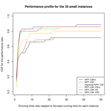
Figure 9: Performance profile [31] showing the Cumulative Distribution Function (CDF) for the performance ratio $r_{\phi,m}$ comparing the running times of all MIP models in the evaluation of the small problem instances.

Table 3: Terminating gap $(\frac{UB-LB}{UB})$ and running time in seconds obtained by the MIP models in the evaluation of all large problem instances. All models were implemented into the same software library based on Gurobi 9.5 onto an UBUNTU 20.04 computer. Time Limit (TL) was set to 3600 seconds, but none model was able to solve any instance up to optimality within this time limit. The ’X’ symbol denotes that no feasible solution was obtained. Best gap results are shown in bold.

		NFP-CMnc	NFP-CM	Improved NFP-CM	NFP-CM-VSnc	NFP-CM-VS	NFP-CM-VS2
Instance	#	GAP	GAP	GAP	GAP	GAP	GAP
Blaz2-16	16	0.299	0.285	0.322	0.304	0.302	0.312
Blaz2	20	0.265	0.271	0.296	0.269	0.265	0.281
Mao	20	0.243	0.285	X	0.798	0.297	X
Albano	24	0.235	0.241	X	0.259	0.19	0.25
Marques	24	0.176	0.207	X	X	0.188	0.179
Jakobs1	25	0.167	0.167	0.167	0.167	0.167	0.167
Jakobs2	25	0.321	0.296	0.367	0.321	0.321	0.269
Blaz1	28	0.243	0.236	X	0.262	0.232	0.264
Dagli	30	0.278	0.249	X	X	0.27	0.215
Shapes0	48	X	X	X	X	X	X
Trousers	64	0.235	0.241	X	X	X	X

5 Discussion

5.1 Comparison in small problem instances

The entire family of NFP-CM-VS models obtains a significantly higher performance ratio than the family of NFP-CM models, and significantly outperforms the baseline Improved NFP-CM model, as shown in figure 9. Likewise, the NFP-CM-VSnc and NFP-CM-VS models solve the largest number of small problem instances up to optimality, as shown in table 2.

The symmetry-breaking proposed by our new geometric decomposition based on vertical slices significantly outperforms that proposed by the baseline Improved NFP-CM model, as shown in figure 9, and the results reported for large problem instances in table 3, in which the NFP-CM-VS and NFP-CM-VS2 models obtain better terminating gaps than the Improved NFP-CM model in all large instances, moreover doubling the number of instances in which a feasible solution is obtained.

Looking at the results in table 2, we find that among the small instances solved up to optimality, NFP-CM-VS2 is the fastest model in 7 instances, whilst NFP-CM-VS, NFP-VSnc, and NFP-CMnc models are the fastest ones in 6 instances, NFP-CM in 5, and Improved NFP-CM in 2.

The NFP-CM-VS and NFP-CM-VSnc models obtain a slightly better performance ratio than the NFP-CM-VS2 model, as shown in figure 9. Thus, the compact formulation of the NFP-CM-VS2 model is unable to outperform the NFP-CM-VS models. Despite our NFP-CM-VS2 model defining a much more compact formulation than the NFP-CM-VS models and removing almost two-thirds of constraints and big-M terms, not only does NFP-CM-VS2 not improve on the NFP-CM-VS models, but it also performs slightly worse than the later ones. Thus, we conjecture that the NFP-CM-VS formulation provides a more tightened model than the more compact NFP-CM-VS2 formulation, making the B&C exploration of the MIP solver faster.

5.2 Comparison in large problem instances

The entire family of NFP-CM-VS models obtains lower terminating gaps than the baseline Improved NFP-CM model in the evaluation of large problem instances. Moreover, our new family of MIP models doubles the cases in which it can find feasible solutions, as shown in table 3.

Current state-of-the-art MIP models evaluated herein are unable to either solve a large instance up to optimality or obtain feasible solutions for all of them, as shown in table 3. NFP-CMnc and NFP-CM models obtain feasible solutions for 10 of 11 large problem instances, whilst NFP-CM-VS does it for 9 cases, NFP-CM-V2 for 8, NFP-CM-VSnc for 7, and the Improved NFP-CM for only 4.

The NFP-CMnc obtains the lowest terminating gap in 4 large problem instances, whilst NFP-CM-VS does it in 3 cases, NFP-CM-VS2 in 2, and NFP-CM in 1, as shown in table 3.

NFP-CM and NFP-CMnc models significantly outperform the baseline Improved NFP-CM model in the large problem instances, as shown in table 3. Table 3 also shows that Improved NFP-CM fails in obtaining feasible solutions in most of instances and it outperform NFP-CM model in none large instance. Thus, the symmetry-breaking proposed by the Improved NFP-CM is unable to provide consistent performance results in the large problems instances in comparison with its results in the small ones.

NFP-CMnc obtains competitive performance results in the large problem instances regarding NFP-CM, despite it have not been evaluated before, as shown in table 3. This conclusion is relevant because despite the introductory paper of Cherri et al. [25] omitted the evaluation of NFP-CMnc in the large problem instances, our results show that there is no a significant difference in performance between NFP-CMnc and NFP-CM, both in small and large problem instances, as shown in figure 9 and table 3.

5.3 Impact of valid cuts among three pieces

The valid cuts among three pieces implemented by our NFP-CM-VS model significantly improve the performance of the NFP-CM-VSnc model. This conclusion can be drawn by comparing the performance profiles shown in figure 9 and the termination gap values reported in table 3 for both former models. Looking at the columns of both aforementioned models in table 3, you can see that NFP-CM-VS obtains a lower or equal terminating gap than NFP-CM-VSnc in all instances in which at least a feasible solution is found. Moreover, NFP-CM-VS finds feasible solutions for two large instances more than NFP-CM-VSnc. Thus, these performance improvements can only be attributed to the single difference between both former models: the valid cuts among three pieces defined by inequalities (41).

5.4 Impact of technological advances and confirmation of previous results

Our replication of all MIP models evaluated herein allows confirming previous results and drawing some conclusions on the impact of the technological advances both in hardware and MIP solvers regarding the results reported by Cherri et al. [25] and Rodrigues et al. [73], regardless our experiments are based on Gurobi 9.5 (2022) instead of the CPLEX 12.6 solver used by the former authors.

The Improved NFP-CM baseline model obtains a higher performance ratio than the NFP-CM and NFP-CMnc models in the evaluation of small problem instances, as shown in figure 9. First, this conclusion allows confirming in a sound way that the Improved NFP-CM sets the current state-of-the-art of the problem, and thus, it sets our baseline for comparison. We note that the Improved NFP-CM model introduced by Rodrigues et al. [73] was not evaluated in the same set of problem instances than the NFP-CM model [25], such as done here for the first time. On the contrary, the Improved NFP-CM model was evaluated in a different and more reduced set of instances, which limits the scope of previous conclusions. However, we bridge this minor gap here by independently confirming the achievements of the family of NFP-CM models [25, 73] in a more sound way.

The Dighe1 instance is solved for the first time up to the optimality by the NFP-CMnc, NFP-CM, NFP-CM-VSnc, and NFP-CM-VS models. This conclusion can be drawn by looking the results reported for the Dighe1 instance in table 2 and comparing them with the results reported in [25, table 1].

The advances in hardware and MIP solvers contribute to improve the performance of NFP-CMnc and NFP-CM models. This conclusion can be drawn by looking the results reported in tables 2 and 3, and comparing them with those reported in [25, tables 1-2]. For instance, NFP-CMnc and NFP-CM are able to solve for the first time the threep3, J1-10-20-3, fu, and Dighe1 instances. However, NFP-CM cannot solve the Shapes8 and threep3w9 instances up to the optimality in our experiments, which we attribute to differences in B&C algorithms of the MIP solvers and the implementation of some valid inequalities using SOS-1 type constraints, as detailed in table 1. On the other hand, this technology improvement is much more noticeable in the case of the large problem instances reported in table 3, in which NFP-CM significantly reduce the terminating gap in all instances and it is able to obtain for the first time a feasible solution for the Trousers instance.

5.5 The new state of the art

Our NFP-CM-VS model sets the new state-of-the-art among the family of continuous MIP models for nesting and provides a more consistent performance ratio than current state-of-the-art models, as shown in figure 9 and tables 2 and 3. Although NFP-CM-VS only obtains comparable results to that obtained by the NFP-CMnc and NFP-CM models in terms of terminating gap in the evaluation of large problem instances, in which NFP-CMnc has the advantage of having one third less constraints than NFP-CM-VS, which significantly reduces the resolution of LP problems during the B&C exploration, the performance ratios reported in figure 9 show that all improvements proposed in the formulation of our NFP-CM-VS models improve the state-of-the-art and suggest new lines of improvement for the problem. Moreover, NFP-CM-VS shows consistent performance results in the full range of problem instances evaluated herein, unlike the Improved NFP-CM model whose performance significantly decreases in the large problem instances.

6 Conclusions and future work

We have introduced a new family of continuous MIP models for irregular strip packing with two different formulations, abbreviated NFP-CM-VS and NFP-CM-VS2, which is based on a new convex decomposition of the feasible regions between convex parts into vertical slices, together with a new family of valid inequalities, symmetry breakings, and variable eliminations derived from the former geometric decomposition.

Our new family of MIP models outperform the state-of-the-art family of NFP-CM models introduced by Cherri et al. [25] and Rodrigues et al. [73]. Our new NFP-CM-VS model significantly and consistently sets the new state of the art of the problem. We show that our new geometric decomposition based on vertical slices outperforms the symmetry-breaking proposed by the Improved NFP-CM model [73], despite NFP-CM-VS tripling the number of constraints of NFP-CM [25] instead of only doubling it as done by the Improved NFP-CM model. Likewise, we show that our new family of valid cuts among three pieces significantly contribute to the performance gain of our NFP-CM-VS model.

Another significant contribution is the introduction of the first confirmatory and reproducible experimental survey in this line of research, which is based on our software implementation of all models evaluated herein into a same Java software library, together with a detailed reproducibility protocol and dataset provided as supplementary material to allow the exact replication of all our models, experiments, and results.

We confirm the previous achievements of the family of NFP-CM models [25], setting the outperformance of the Improved NFP-CM model [73] on the former ones in a sound way by replicating all models from scratch and comparing them in the same benchmark reported by Cherri et al. [25].

As forthcoming activities, we plan to study the proposal of any decomposition method or matheuristics that allows improve the performance of our new family of MIP models for nesting.

Acknowledgements

We are grateful to Luiz Cherri, Ramón Álvarez-Valdés, and Antonio Martínez-Sykora for providing us the problem instances used in their benchmarks, and to Alicia Lara-Clares by testing our reproducibility protocol.

Appendix A Appendix A: Raw output data for all models

This appendix introduces all raw output data generated by our experiments not reported herein by lack of room.

Appendix B Appendix B: The reproducible experiments on irregular strip-packing

This appendix introduces a detailed reproducibility protocol and dataset [50] providing our raw output data together with a collection of software and data resources to allow the exact replication of all our experiments and results.

References

- Adamowicz and Albano [1976a] Adamowicz, M., Albano, A., 1976a. Nesting two-dimensional shapes in rectangular modules. Comput. Aided Des. Appl. 8, 27–33.
- Adamowicz and Albano [1976b] Adamowicz, M., Albano, A., 1976b. A solution of the rectangular Cutting-Stock problem. IEEE Trans. Syst. Man Cybern. SMC-6, 302–310.
- Agarwal et al. [2002] Agarwal, P.K., Flato, E., Halperin, D., 2002. Polygon decomposition for efficient construction of Minkowski sums. Computational geometry: theory and applications 21, 39–61.
- Al Theeb et al. [2021] Al Theeb, N.A., Hayajneh, M.T., Jaradat, M.Y., 2021. New strategy to improve the dotted board model for solving two dimensional cutting and packing problems. Computers & Industrial Engineering 159, 107467.
- Albano and Sapuppo [1980] Albano, A., Sapuppo, G., 1980. Optimal allocation of Two-Dimensional irregular shapes using heuristic search methods. Systems, Man and Cybernetics, IEEE Transactions on 10, 242–248.
- Alvarez-Valdes et al. [2013] Alvarez-Valdes, R., Martinez, A., Tamarit, J.M., 2013. A branch & bound algorithm for cutting and packing irregularly shaped pieces. Int. J. Prod. Econ. 145, 463–477.
- Álvarez-Valdés et al. [2009] Álvarez-Valdés, R., Parreño, F., Tamarit, J.M., 2009. A branch and bound algorithm for the strip packing problem. OR Spectrum. Quantitative Approaches in Management 31, 431–459.
- Alves et al. [2012] Alves, C., Brás, P., Valério de Carvalho, J., Pinto, T., 2012. New constructive algorithms for leather nesting in the automotive industry. Computers & operations research 39, 1487–1505.
- Amaro Júnior et al. [2017] Amaro Júnior, B., Pinheiro, P.R., Coelho, P.V., 2017. A parallel biased Random-Key genetic algorithm with multiple populations applied to irregular strip packing problems. Math. Probl. Eng. 2017.
- Annamalai Vasantha et al. [2016] Annamalai Vasantha, G.V., Jagadeesan, A.P., Corney, J.R., Lynn, A., Agrawal, A., 2016. Crowdsourcing solutions to 2D irregular strip packing problems from internet workers. Int. J. Prod. Res. 54, 4104–4125.
- Art [1966] Art, Jr, R.C., 1966. An approach to the two dimensional irregular cutting stock problem. Ph.D. thesis. Massachusetts Institute of Technology.
- Bennell and Oliveira [2008] Bennell, J.A., Oliveira, J.F., 2008. The geometry of nesting problems: A tutorial. Eur. J. Oper. Res. 184, 397–415.
- Bennell and Oliveira [2009] Bennell, J.A., Oliveira, J.F., 2009. A tutorial in irregular shape packing problems. J. Oper. Res. Soc. , S93–S105.
- Bennell et al. [2013] Bennell, J.A., Oliveira, J.F., Wäscher, G., 2013. Cutting and packing. International Journal of Production Economics 145, 449–450.
- de Berg et al. [1997] de Berg, M., Van Kreveld, M., Overmars, M., Schwarzköpf, O., 1997. Computational Geometry: Algorithms and Applications. Springer-Verlag.
- Carravilla and Ribeiro [2005] Carravilla, M.A., Ribeiro, C., 2005. CP and MIP in the resolution of hard combinatorial problems: A case study with nesting problems, in: Proceedings of the CSCLP 2005 Joint ERCIM/CoLogNET International Workshop on Constraint Solving and Constraint Logic Programming, Citeseer, Uppsala, Sweden. pp. 113–127.
- Carravilla et al. [2003] Carravilla, M.A., Ribeiro, C., Oliveira, J.F., 2003. Solving nesting problems with non-convex polygons by constraint logic programming. Int. Trans. Oper. Res. 10, 651–663.
- Cheok and Nee [1991] Cheok, B.T., Nee, A.Y.C., 1991. Algorithms for nesting of ship/offshore structural plates. American Society of Mechanical Engineers, Design Engineering Division (Publication) DE 32, 221–226.
- Chernov et al. [2010] Chernov, N., Stoyan, Y., Romanova, T., 2010. Mathematical model and efficient algorithms for object packing problem. Comput. Geom. 43, 535–553.
- Chernov et al. [2012] Chernov, N., Stoyan, Y., Romanova, T., Pankratov, A., 2012. Phi-Functions for 2D Objects Formed by Line Segments and Circular Arcs. Advances in Operations Research 2012.
- Cherri et al. [2019] Cherri, L.H., Carravilla, M.A., Ribeiro, C., Toledo, F.M.B., 2019. Optimality in nesting problems: New constraint programming models and a new global constraint for non-overlap. Operations Research Perspectives 6, 100125.
- Cherri et al. [2016a] Cherri, L.H., Carravilla, M.A., Toledo, F.M.B., 2016a. A MODEL-BASED HEURISTIC FOR THE IRREGULAR STRIP PACKING PROBLEM. Pesquisa Operacional 36, 447–468.
- Cherri et al. [2018a] Cherri, L.H., Cherri, A.C., Carravilla, M.A., Oliveira, J.F., Toledo, F.M.B., Vianna, A.C.G., 2018a. An innovative data structure to handle the geometry of nesting problems. International Journal of Production Research 56, 7085–7102.
- Cherri et al. [2018b] Cherri, L.H., Cherri, A.C., Soler, E.M., 2018b. Mixed integer quadratically-constrained programming model to solve the irregular strip packing problem with continuous rotations. J. Global Optimiz. 72, 89–107.
- Cherri et al. [2016b] Cherri, L.H., Mundim, L.R., Andretta, M., Toledo, F.M.B., Oliveira, J.F., Carravilla, M.A., 2016b. Robust mixed-integer linear programming models for the irregular strip packing problem. European Journal of Operational Research 253, 570–583.
- Codato and Fischetti [2006] Codato, G., Fischetti, M., 2006. Combinatorial Benders’ Cuts for Mixed-Integer Linear Programming. Operations research 54, 756–766.
- Conte et al. [2020] Conte, A., Grossi, R., Marino, A., 2020. Large-scale clique cover of real-world networks. Information and Computation 270, 104464.
- Cuninghame-Green [1989] Cuninghame-Green, R., 1989. Geometry, shoemaking and the milk tray problem. New scientist 123, 50–53.
- Daniels et al. [1994] Daniels, K., Li, Z., Milenkovic, V., 1994. Multiple containment methods. Technical Report Technical Report TR-12-94. Harvard Computer Science Group.
- Dean [2002] Dean, H.T., 2002. Minimizing waste in the 2-dimensional cutting stock problem. Ph.D. thesis. Department of Mechanical Engineering, University of Canterbury. Christchurch, New Zealand.
- Dolan and Moré [2002] Dolan, E.D., Moré, J.J., 2002. Benchmarking optimization software with performance profiles. Mathematical Programming. A Publication of the Mathematical Programming Society 91, 201–213.
- Dowsland and Dowsland [1992] Dowsland, K.A., Dowsland, W.B., 1992. Packing problems. Eur. J. Oper. Res. 56, 2–14.
- Dowsland and Dowsland [1995] Dowsland, K.A., Dowsland, W.B., 1995. Solution approaches to irregular nesting problems. Eur. J. Oper. Res. 84, 506–521.
- Dowsland et al. [2002] Dowsland, K.A., Vaid, S., Dowsland, W.B., 2002. An algorithm for polygon placement using a bottom-left strategy. European Journal of Operational Research 141, 371–381.
- Dyckhoff [1990] Dyckhoff, H., 1990. A typology of cutting and packing problems. Eur. J. Oper. Res. 44, 145–159.
- Elamvazuthi et al. [2009] Elamvazuthi, I., Kamaruddin, S., Azmi, M.S., 2009. Automation of nesting and cutting processes of leather furniture production: a case study. International Journal of Mechanical & Mechatronics Engineering IJMME 9.
- Elkeran [2013] Elkeran, A., 2013. A new approach for sheet nesting problem using guided cuckoo search and pairwise clustering. Eur. J. Oper. Res. 231, 757–769.
- Fernández et al. [2000] Fernández, J., Cánovas, L., Pelegrín, B., 2000. Algorithms for the decomposition of a polygon into convex polygons. European Journal of Operational Research 121, 330–342.
- Fischetti and Luzzi [2009] Fischetti, M., Luzzi, I., 2009. Mixed-integer programming models for nesting problems. Journal of Heuristics 15, 201–226.
- Fowler et al. [1981] Fowler, R.J., Paterson, M.S., Tanimoto, S.L., 1981. Optimal packing and covering in the plane are NP-complete. Inf. Process. Lett. 12, 133–137.
- Gilmore and Gomory [1965] Gilmore, P.C., Gomory, R.E., 1965. Multistage cutting stock problems of two and more dimensions. Oper. Res. 13, 94–120.
- Gomes and Oliveira [2002] Gomes, A.M., Oliveira, J.F., 2002. A 2-exchange heuristic for nesting problems. Eur. J. Oper. Res. 141, 359–370.
- Greene [1983] Greene, D.H., 1983. The decomposition of polygons into convex parts, in: Preparata, F. (Ed.), Computational Geometry. JAI Press, Greenwich, Connecticut (USA).. volume 1 of Adv. Comput. Res., pp. 235–259.
- Han et al. [2013] Han, W., Bennell, J.A., Zhao, X., Song, X., 2013. Construction heuristics for two-dimensional irregular shape bin packing with guillotine constraints. Eur. J. Oper. Res. 230, 495–504.
- Heistermann and Lengauer [1995] Heistermann, J., Lengauer, T., 1995. The nesting problem in the leather manufacturing industry. Ann. Oper. Res. .
- Hopper and Turton [2001] Hopper, E., Turton, B.C.H., 2001. A review of the application of Meta-Heuristic algorithms to 2D strip packing problems. Artificial Intelligence Review 16, 257–300.
- Iori et al. [2021] Iori, M., de Lima, V.L., Martello, S., Miyazawa, F.K., Monaci, M., 2021. Exact solution techniques for two-dimensional cutting and packing. European Journal of Operational Research 289, 399–415.
- Jones [2014] Jones, D.R., 2014. A fully general, exact algorithm for nesting irregular shapes. J. Global Optimiz. 59, 367–404.
- Kallrath [2009] Kallrath, J., 2009. Cutting circles and polygons from area-minimizing rectangles. Journal of Global Optimization 43, 299–328.
- Lastra-Díaz and Ortuño [2022] Lastra-Díaz, J.J., Ortuño, M.T., 2022. Reproducibility dataset for a new mixed-integer programming model for irregular strip packing based on vertical slices. Mendeley Data, V1, doi:10.17632/m8nzsk5c9v.1. http://dx.doi.org/10.17632/m8nzsk5c9v.1.
- Leao and Toledo [2021] Leao, A.A.S., Toledo, F.M.B., 2021. Enhanced solution for the irregular strip packing problem: valid inequalities and branching priorities, in: LIII Simpósio Brasileiro de Pesquisa Operacional Joao Pessoa, pp. 1–12.
- Leao et al. [2016] Leao, A.A.S., Toledo, F.M.B., Oliveira, J.F., Carravilla, M.A., 2016. A semi-continuous MIP model for the irregular strip packing problem. International Journal of Production Research 54, 712–721.
- Leao et al. [2020] Leao, A.A.S., Toledo, F.M.B., Oliveira, J.F., Carravilla, M.A., Álvarez-Valdés, R., 2020. Irregular packing problems: A review of mathematical models. European Journal of Operational Research 282, 803–822.
- Li [1994] Li, Z., 1994. Compaction algorithms for non-convex polygons and their applications. Ph.D. thesis. Harvard University. http://nrs.harvard.edu/urn-3:HUL.InstRepos:25619464.
- Li and Milenkovic [1993] Li, Z., Milenkovic, V., 1993. A compaction algorithm for non-convex polygons and its application, in: Proceedings of the Ninth Annual Symposium on Computational Geometry, ACM, New York, NY, USA. pp. 153–162.
- Li and Milenkovic [1995] Li, Z., Milenkovic, V., 1995. Compaction and separation algorithms for non-convex polygons and their applications. Eur. J. Oper. Res. 84, 539–561.
- Lodi et al. [2002] Lodi, A., Martello, S., Vigo, D., 2002. Recent advances on two-dimensional bin packing problems. Discrete Appl. Math. 123, 379–396.
- Milenkovic et al. [1991] Milenkovic, V., Daniels, K., Li, Z., 1991. Automatic marker making, in: Proceedings of the Third Canadian Conference on Computational Geometry, nereida.deioc.ull.es. pp. 243–246.
- Moore [1966] Moore, R.E., 1966. Interval analysis. Prentice Hall.
- Moore et al. [2009] Moore, R.E., Kearfott, R.B., Cloud, M.J., 2009. Introduction to INTERVAL ANALYSIS. volume 2. Society for Industrial and Applied Mathematics (SIAM).
- Mundim et al. [2018] Mundim, L.R., Andretta, M., Carravilla, M.A., Oliveira, J.F., 2018. A general heuristic for two-dimensional nesting problems with limited-size containers. Int. J. Prod. Res. 56, 709–732.
- Mundim et al. [2017] Mundim, L.R., Andretta, M., de Queiroz, T.A., 2017. A biased random key genetic algorithm for open dimension nesting problems using no-fit raster. Expert Syst. Appl. 81, 358–371.
- Pankratov et al. [2020] Pankratov, A., Romanova, T., Shekhovtsov, S., Grebennik, I., Pankratova, J., 2020. Packing Irregular Polygons using Quasi Phi-functions, in: 2020 10th International Conference on Advanced Computer Information Technologies (ACIT), pp. 1–5.
- Peralta et al. [2018] Peralta, J., Andretta, M., Oliveira, J.F., 2018. SOLVING IRREGULAR STRIP PACKING PROBLEMS WITH FREE ROTATIONS USING SEPARATION LINES. Pesqui. Oper. 38, 195–214.
- Pinheiro et al. [2016] Pinheiro, P.R., Amaro Júnior, B., Saraiva, R.D., 2016. A random-key genetic algorithm for solving the nesting problem. Int. J. Comput. Integr. Manuf. 29, 1159–1165.
- Puri [2013] Puri, A., 2013. Efficacy of Pattern Making Software in Product Development. International Journal of Advanced Quality Management 1, 21–39.
- Ribeiro and Carravilla [2004] Ribeiro, C., Carravilla, M.A., 2004. A global constraint for nesting problems, in: Integration of AI and OR Techniques in Constraint Programming for Combinatorial Optimization Problems, Springer Berlin Heidelberg. pp. 256–270.
- Ribeiro and Carravilla [2009] Ribeiro, C., Carravilla, M.A., 2009. A global constraint for nesting problems. Artificial Intelligence Review 30, 99.
- Ribeiro et al. [1999] Ribeiro, C., Carravilla, M.A., Oliveira, J.F., 1999. Applying constraint logic programming to the resolution of nesting problems. Pesquisa Operacional 19, 239–247.
- Riff et al. [2009] Riff, M.C., Bonnaire, X., Neveu, B., 2009. A revision of recent approaches for two-dimensional strip-packing problems. Engineering applications of artificial intelligence 22, 823–827.
- Rocha et al. [2016] Rocha, P., Gomes, A.M., Rodrigues, R., Toledo, F.M.B., Andretta, M., 2016. Constraint Aggregation in Non-linear Programming Models for Nesting Problems, in: Computational Management Science, Springer International Publishing. pp. 175–180.
- Rocha et al. [2014] Rocha, P., Rodrigues, R., Gomes, A.M., Toledo, F.M.B., Andretta, M., 2014. Circle Covering Representation for Nesting problems with continuous rotations. IFAC Proceedings Volumes. Proc. of the 19th IFAC World Congress 47, 5235–5240.
- Rodrigues et al. [2017] Rodrigues, M.O., Cherri, L.H., Mundim, L.R., 2017. MIP models for the irregular strip packing problem: new symmetry breaking constraints. ITM Web of Conferences 14, 00005.
- Rodrigues and Toledo [2017] Rodrigues, M.O., Toledo, F.M.B., 2017. A clique covering MIP model for the irregular strip packing problem. Comput. Oper. Res. 87, 221–234.
- Romanova et al. [2020] Romanova, T., Stoyan, Y., Pankratov, A., Litvinchev, I., Marmolejo, J.A., 2020. Decomposition Algorithm for Irregular Placement Problems, in: Intelligent Computing and Optimization, Springer International Publishing. pp. 214–221.
- Santoro and Lemos [2015] Santoro, M.C., Lemos, F.K., 2015. Irregular packing: MILP model based on a polygonal enclosure. Ann. Oper. Res. 235, 693–707.
- Sato et al. [2019] Sato, A.K., Martins, T.C., Gomes, A.M., Tsuzuki, M.S.G., 2019. Raster penetration map applied to the irregular packing problem. European Journal of Operational Research 279, 657–671.
- Sato et al. [2016a] Sato, A.K., Martins, T.d.C., Tsuzuki, M.d.S.G., 2016a. A pairwise exact placement algorithm for the irregular nesting problem. International Journal of Computer Integrated Manufacturing 29, 1177–1189.
- Sato et al. [2016b] Sato, A.K., de Sales Guerra Tsuzuki, M., de Castro Martins, T., Gomes, A.M., 2016b. Study of the grid size impact on a raster based strip packing problem solution. IFAC-PapersOnLine 49, 143–148.
- Sawaya and Grossmann [2005] Sawaya, N.W., Grossmann, I.E., 2005. A cutting plane method for solving linear generalized disjunctive programming problems. Computers & chemical engineering 29, 1891–1913.
- Rodrigues de Souza and Andretta [2020] Rodrigues de Souza, L., Andretta, M., 2020. Modelo de programaçao estocástica para um problema de corte de itens irregulares, in: LII Simpósio Brasileiro de Oesquisa Operacional.
- Rodrigues de Souza and Andretta [2022] Rodrigues de Souza, L., Andretta, M., 2022. A branch-and-cut algorithm for the irregular strip packing problem with uncertain demands. International transactions in operational research: a journal of The International Federation of Operational Research Societies .
- Stoyan et al. [2016a] Stoyan, Y., Pankratov, A., Romanova, T., 2016a. Cutting and packing problems for irregular objects with continuous rotations: mathematical modelling and non-linear optimization. The Journal of the Operational Research Society 67, 786–800.
- Stoyan et al. [2016b] Stoyan, Y., Pankratov, A., Romanova, T., 2016b. Quasi-phi-functions and optimal packing of ellipses. Journal of Global Optimization 65, 283–307.
- Stoyan et al. [2017] Stoyan, Y., Pankratov, A., Romanova, T., 2017. Placement Problems for Irregular Objects: Mathematical Modeling, Optimization and Applications, in: Butenko, S., Pardalos, P.M., Shylo, V. (Eds.), Optimization Methods and Applications : In Honor of Ivan V. Sergienko’s 80th Birthday. Springer International Publishing, Cham, pp. 521–559.
- Stoyan and Romanova [2013] Stoyan, Y., Romanova, T., 2013. Mathematical Models of Placement Optimisation: Two- and Three-Dimensional Problems and Applications, in: Fasano, G., Pintér, J.D. (Eds.), Modeling and Optimization in Space Engineering. Springer New York, New York, NY, pp. 363–388.
- Stoyan et al. [2015] Stoyan, Y., Romanova, T., Pankratov, A., Chugay, A., 2015. Optimized Object Packings Using Quasi-Phi-Functions, in: Fasano, G., Pintér, J.D. (Eds.), Optimized Packings with Applications. Springer International Publishing, Cham, pp. 265–293.
- Stoyan et al. [1996] Stoyan, Y.G., Novozhilova, M.V., Kartashov, A.V., 1996. Mathematical model and method of searching for a local extremum for the non-convex oriented polygons allocation problem. European Journal of Operational Research 92, 193–210.
- Stoyan et al. [2012] Stoyan, Y.G., Zlotnik, M.V., Chugay, A.M., 2012. Solving an optimization packing problem of circles and non-convex polygons with rotations into a multiply connected region. The Journal of the Operational Research Society 63, 379–391.
- Sweeney and Paternoster [1992] Sweeney, P.E., Paternoster, E.R., 1992. Cutting and packing problems: A categorized, Application-Orientated research bibliography. J. Oper. Res. Soc. 43, 691–706.
- Toledo et al. [2013] Toledo, F.M.B., Carravilla, M.A., Ribeiro, C., Oliveira, J.F., Gomes, A.M., 2013. The Dotted-Board model: A new MIP model for nesting irregular shapes. Int. J. Prod. Econ. 145, 478–487.
- Wang et al. [2018] Wang, A., Hanselman, C.L., Gounaris, C.E., 2018. A customized branch-and-bound approach for irregular shape nesting. J. Global Optimiz. 71, 935–955.
- Wang and Wäscher [2002] Wang, P.Y., Wäscher, G., 2002. Cutting and packing. European Journal of Operational Research 141, 239–240.
- Wäscher et al. [2007] Wäscher, G., Haußner, H., Schumann, H., 2007. An improved typology of cutting and packing problems. Eur. J. Oper. Res. 183, 1109–1130.
- Whelan and Batchelor [1993] Whelan, P.F., Batchelor, B.G., 1993. Automated packing systems: Review of industrial implementations. Mach. Vis. Appl. .