Solar-to-supersolar sodium and oxygen absolute abundances for
a “hot Saturn” orbiting a metal-rich star

Abstract

We present new analysis of infrared transmission spectroscopy of the cloud-free hot-Saturn WASP-96b performed with the Hubble and Spitzer Space Telescopes (HST and Spitzer). The WASP-96b spectrum exhibits the absorption feature from water in excellent agreement with synthetic spectra computed assuming a cloud-free atmosphere. The HST-Spitzer spectrum is coupled with Very Large Telescope (VLT) optical transmission spectroscopy which reveals the full pressure-broadened profile of the sodium absorption feature and enables the derivation of absolute abundances. We confirm and correct for a spectral offset of $\Delta R_{{\rm p}}/R_{\ast}=(-4.29^{+0.31}_{-0.37})\,\times 10^{-3}$ of the VLT data relative to the HST-Spitzer spectrum. This offset can be explained by the assumed radius for the common-mode correction of the VLT spectra, which is a well-known feature of ground-based transmission spectroscopy. We find evidence for a lack of chromospheric and photometric activity of the host star which, therefore, make a negligible contribution to the offset. We measure abundances for Na and O that are consistent with solar to supersolar, with abundances relative to solar values of $21^{+27}_{-14}$ and $7^{+11}_{-4}$, respectively. We complement the transmission spectrum with new thermal emission constraints from Spitzer observations at 3.6 and $4.5\mu$m, which are best explained by the spectrum of an atmosphere with a temperature decreasing with altitude. A fit to the spectrum assuming an isothermal blackbody atmosphere constrains the dayside temperature to be $T_{\rm{p}}$=$1545$$\pm$$90$K.

1 Introduction

From massive gas-giants down to Earth-mass worlds, from ultra-hot planets to much cooler and potentially habitable Earth-like analogs, exoplanets have now been found orbiting many of the stars across the solar neighborhood. Following nearly three decades of exoplanet detections, the exoplanet census now shows that planet formation is ubiquitous with Super-Earths being common and hot Jupiters, planets similar to Jupiter in the Solar System but with orbital periods shorter than about 10 days, uncommon (Burke et al., 2015; Wang et al., 2015; Howard et al., 2010, 2012; Mayor et al., 2011; Brewer et al., 2016). Due to their large radii and hot temperatures, hot Jupiters host the only class of exoplanet atmosphere that can currently be observationally characterized in detail with spectroscopic observations over an entire orbital phase Fortney et al. (2021). Even the first steps to characterize exoplanets via transits have started to reveal astoundingly diverse worlds very different from the planets of the Solar System with: (i) evaporating and escaping planetary atmospheres resembling comet-like tails (Ehrenreich et al., 2015); (ii) atmospheric hazes and clouds composed of minerals and metal oxides, which tend to be ubiquitous (Lecavelier Des Etangs et al., 2008; Sing et al., 2013; Huitson et al., 2013; Nikolov et al., 2015; Carter et al., 2020; Alam et al., 2020; Spyratos et al., 2021; Wilson et al., 2020); and (iii) a huge diversity and a continuum from clear to cloudy atmospheres (Sing et al., 2016; Gibson et al., 2017; Wakeford et al., 2018; Evans et al., 2018; Alam et al., 2021; Fu et al., 2021; Spake et al., 2021; Sheppard et al., 2021). From all types, exoplanet atmospheres free of clouds offer a unique opportunity to constrain elemental abundances (e.g., Na, K, water and carbon-bearing molecules and metallicity objectively), as clouds and hazes obscure the amplitudes of absorption features (Fortney, 2005; Fortney et al., 2010). Such rare exoplanets enable unbiased absolute abundance constraints, which may inform theory of irradiated gas-giant exoplanet atmospheres and giant planet formation (Öberg et al., 2011; Madhusudhan, 2012; Madhusudhan et al., 2017). Because the composition of protoplanetary disks vary significantly with distance from the star, an exoplanet’s atmospheric composition may contain a fossil record of the conditions of the disk at the location where the planet formed. Madhusudhan (2012) showed that the C/O ratio carries important information on the chemistry of volatile species, which has started to provide definitve constraints (Line et al., 2021). Lothringer et al. (2021) explored the insight that the measurement of refractory abundances can provide into a planet’s origins. Through refractory-to-volatile elemental abundance ratios, they demonstrated that a planet’s atmospheric rock-to-ice fraction can be estimated, which can constrain planet formation and migration scenarios.

Motivated by the recent observational results from space and the ground, theoretical predictions for strong alkali features, stratosphere inducing TiO and VO, and diversity of clouds hazes and dust, we initiated a large transmission spectral survey of twenty exoplanets with the FORS spectrograph on the Very Large Telescope (VLT). Optical transmission spectra from this program have been reported for WASP-96b, WASP-103b, WASP-88b and WASP-110b (Nikolov et al., 2018c; Wilson et al., 2020; Spyratos et al., 2021; Nikolov et al., 2021). In this study, we performed follow-up reconnaissance observations of WASP-96b using HST and Spitzer, aiming at detecting water in the transmission spectrum of the planet.

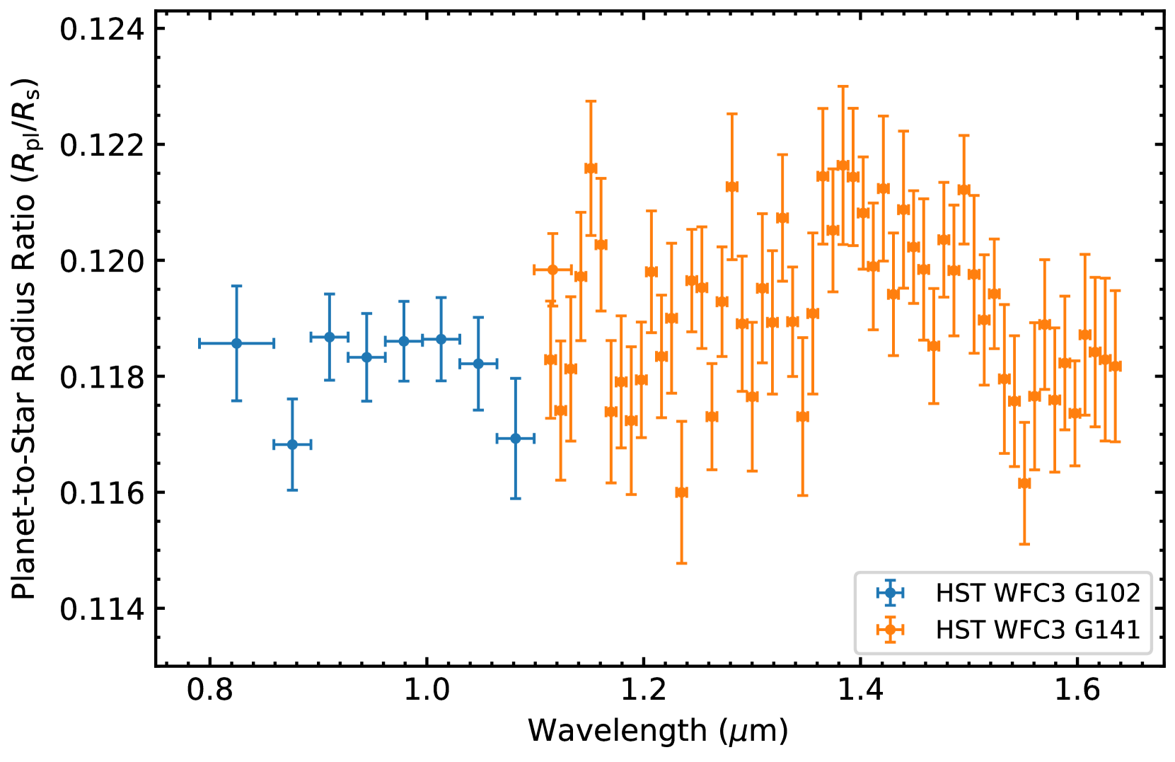
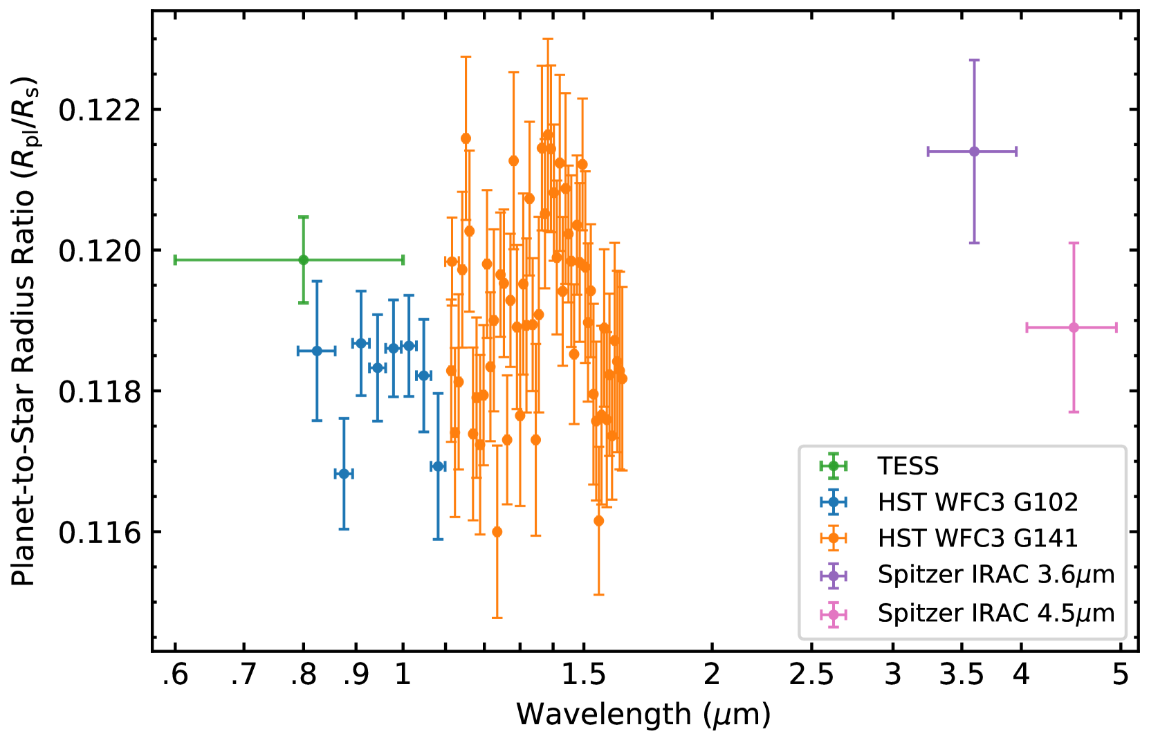
Figure 1: Infrared transmission spectrum of the cloud-free WASP-96b. The error bars indicate the $1\sigma$ uncertainties. Top panel: Results from the two HST WFC3 spectroscopic observations. Lower panel: Combined HST WFC3 transit spectroscopy and TESS and Spitzer IRAC $3.6\mu$m and $4.5\mu$m transit photometry.

WASP-96b is a ”hot Saturn“ with a planetary mass $M_{\rm{p}}=0.48\pm 0.03M_{\rm{J}}$, where $M_{\rm{J}}$ is the mass of Jupiter, planet radius $R_{\rm{p}}=1.20\pm 0.06R_{\rm{J}}$, where $R_{\rm{J}}$ is the radius of Jupiter and an equilibrium temperature $T_{{\rm{eq}}}=1285\pm 40$K on a 3.4-day circular orbit around a ${\mathrm{V}}=12.2$ chromospherically quiet and photometrically stable (Section 3.4) G8 star at a distance of $356\pm 5$ pc in the southern constellation Phoenix (Hellier et al., 2014). Unlike the optical transmission spectrum for a majority of hot Jupiters known to date, the spectrum of WASP-96b shows very clear pressure-broadened wings of the sodium line, evidence of potassium and a near-UV Rayleigh scattering slope, with the latter defining the hydrogen continuum level and proving the planet has a clear atmosphere at the limb. The VLT spectrum provides an absolute sodium abundance, $2-18\times$ the solar value ($1\sigma$) and an atmospheric metallicity in agreement with the mass-metallicity trend observed for solar-system planets and exoplanets (Nikolov et al., 2018c; Thorngren et al., 2016). This suggests that the absorption signature of molecules, such as water with absorption bands at $\sim 0.95$, $1.15$ and $1.4\mu$m, carbon monoxide and methane at $3.6$ and $4.5\mu$m are expected to also be free from the suppressing effect of clouds and hazes in the infrared (Sing et al., 2016). We carried out (i) transit observations with the Hubble Space Telescope (HST) in spatial scanning mode, and (ii) Spitzer Space Telescope (Spitzer) transit and eclipse observations, to extend the planet’s optical transmission spectrum at these wavelengths, constrain the atmospheric composition and day side brightness temperature of the planet (GO-15469 and 14255; Nikolov et al., 2018a, 2019). An analysis of the transit observations has been reported by Yip et al. (2021), finding absorption from water and an offset between the optical and infrared.

In this paper, we present new results for the infrared transmission spectrum, which overall agree with the results from Yip et al. (2021), finding solar to supersolar abundances for sodium and oxygen. We additionally find the planet’s potassium and carbon abundances to be low with broad uncertainties owing to lower precision of the spectrum at the relevant wavelengths. We present new results for the elemental abundances of the host star, its chromospheric activity index, constrain the dayside temperature of the planet and refine the system parameters and planet orbital ephemeris. We demonstrate in this work, as has been detailed in Nikolov et al. (2018c) that the observed offset of the optical spectrum is explained by the assumed absolute planet-to-star radius ratio for the calculation of common mode (wavelength independent) systematics model for the ground-based spectra. As the hot Jupiter with the clearest known atmosphere, WASP-96b is poised to become an important prototype exoplanet target for the James Webb Space Telescope and provide the first accurate abundance measurements, unbiased by clouds and hazes.

We describe the observations in Section 2, discuss the data reduction and light curve analysis in Section 3, present results from a retrieval analysis in Section 4 and discuss our findings in the context of literature result in Section 5 and summarize and conclude in Section 6.

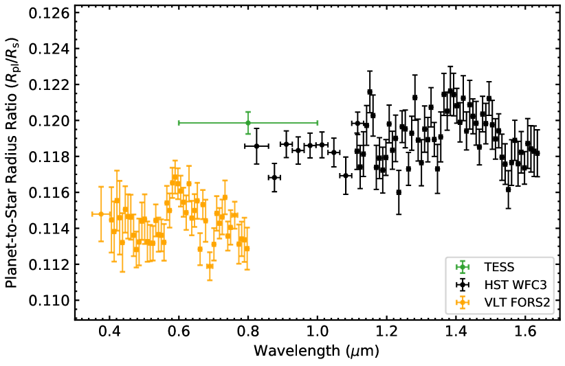
Figure 2: Combined transmission spectrum of WASP-96b. Plotted are the VLT and HST spectra with orange and black symbols, respectively. A radius measurement from a combined analysis of TESS photometric light curves is indicated with the green symbol. Error-bars mark the $1\sigma$ uncertainties.

2 Observations and reductions

2.1 HST WFC3 spatial scan mode transit spectroscopy

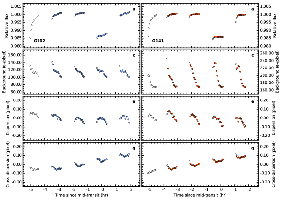
Figure 11: HST WFC3 white light curves and spectroscopic properties. Left and right panels refer to the G102 (blue) and G141 (red) data, respectively. Filled and open symbols, respectively, indicate retained and discarded data in our light-curve analysis. a-b, Normalised raw flux. c-d, Measured background for each frame in units of electrons per pixel, using the last individual read of each full scan. e-f, Median-subtracted drift of the spectra along the dispersion axis in units of pixels, estimated by cross-correlating the spectra with respect to the first spectrum. g-h, Same as the previous panel, but for the cross-dispersion axis measured with flux-weighted mean.

We observed two primary transits of WASP-96b with the Wide Field Camera 3 (WFC3) aboard the Hubble Space Telescope (HST) as part of Program 15469, (Nikolov et al., 2018a) in spatial scan mode. Both visits included five consecutive HST orbits, with the first, second, third and fifth orbits covering out of transit phases and the fourth orbit during the transit. The HST orbital sequence was planned such that the in-transit orbit covers the planet phase between second and third contacts (end of ingress and start of egress, respectively) to maximize the precision of the measured planet radius (Figure 11 and 12). Each observation was performed in spatial scan mode using the $256\times 256$ subarray centered on the target to reduce read-out overheads. The spatial scan mode spreads the stellar flux across more pixels compared to a fixed pointing (stared) observation, allowing for a longer exposure times with higher duty cycle. Prior to the spectral observations, we acquired direct images of the target to facilitate a wavelength solution and to inspect the vicinity of the target for field stars that can contaminate the spectra. We exposed for 1.111 and 1.389s using the F127M and F139M filters for the G102 and G141 grisms, respectively. An inspection of the direct images showed the field around WASP-96 to be free of stars.

The first observation covers the transit on UT 2018 December 18th. We used the dispersive element G102, which covers the spectral range from 0.8 to $1.15\mu$m at a resolving power of $R\sim 210$ (at $1\mu$m) and a dispersion of $2.45$ nm px^-1. We used forward scanning with a rate of 0.013 arcsec sec^-1 and the SPARS25 sampling sequence with eleven iterations per exposure (NSAMP9) resulting in total integration times of $\sim 179$ sec and scans across 2.3 arcsec $(\sim 18$ px$)$. Typical count levels reached a maximum of $\sim 2.9\times 10^{4}$ analogue-to-digital units (ADU), i.e. well within the linear regime of the detector.

The second observation covered the transit on UT 2018 December 28th. We exploited the dispersive element G141, which covers the spectral range from 1.075 to $1.7\mu$m at a resolving power of $R\sim 130$ (at $1.4\mu$m) and a dispersion of $4.65$ nm px^-1. We used forward scanning with a rate of 0.022 arcsec sec^-1 and the SPARS25 sampling sequence with twelve iterations per exposure (NSAMP8) resulting in total integration times of $\sim 157$ sec and scans across 3.4 arcsec $(\sim 268$ px$)$. The spectra reached typical maximum count levels of $\sim 2.8\times 10^{4}$ ADU, i.e. within the linear regime of the detector.

We performed data reduction and analysis following the procedures outlined in Nikolov et al. (2018b). Our analysis started with the 2D ima spectra, produced by the calwf3 pipeline (v3.1), which are corrected for bias, dark current, flat-field and detector non-linearity effects. We extracted flux for WASP-96b from each exposure by taking each successive non-destructive read difference. We removed the background on each individual read difference by taking the median flux in a box away from the stellar spectrum. We then determined the flux weighted centre of the WASP-96 scan and set to zero all pixel values located more than 20 pixels above and below along the cross-dispersion axis. Application of this top hat filter had the effect of eliminating most of the pixels affected by cosmic rays. The final reconstructed images were produced by adding together the read differences for each exposure. Any remaining cosmic rays were identified and corrected, following the procedure described in Nikolov et al. (2014, 2018b). We find a total of 2 or 3 pixels that sample the spectra to be affected by cosmic rays for each reconstructed image.

We performed a spectral extraction using a fixed-size box by summing the flux of all pixels. The box had dimensions of $171\times 28$ and $169\times 39$ pixels for the G102 and G141 data, respectively and centered for each individual exposure. To identify the box positions along the dispersion and cross-dispersion axis we took the flux-weighted mean of each 2D spectrum. The target drift along the dispersion and cross-dispersion axis are shown in Figure 11.

We established wavelength solutions for each grism time series by cross-correlating each spectrum with an ATLAS synthetic stellar spectrum (Kurucz, 1979) that matches the astrophysical properties of the WASP-96 host star i.e., ${\mathrm{T_{\rm{eff}}=5500\pm 150}}$ K, $\log{g}=4.42\pm 0.02$ and ${\mathrm{[Fe/H]}}=0.14\pm 0.19$, reported in Hellier et al. (2014). We obtained synthetic spectra from the HST exposure time calculator, which also accounts for the instrument sensitivity.

2.2 Spitzer IRAC transit and eclipse photometry

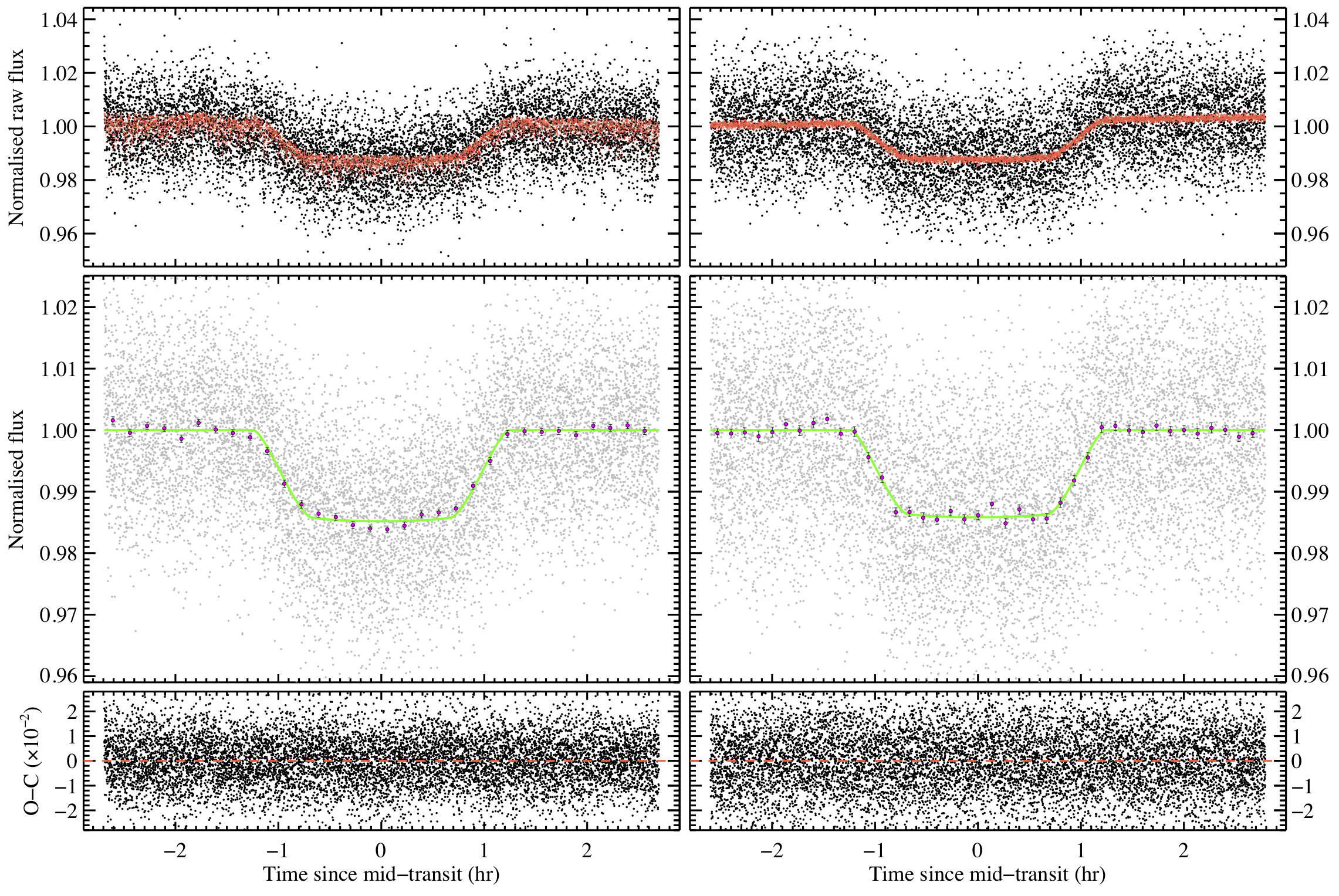
Figure 13: Spitzer  IRAC 3.6 and 4.5 $\mu$m photometry (left and right,respectively).Top panels: raw flux and the best-fitting transit and systematics model; middle panels: detrended light curves and the best-fitting transit models and binned by 8 min; lower panels: light-curve residuals.

Photometric data were collected during two primary transits and two secondary eclipses using the Spitzer Space Telescope ($Spitzer$, Werner et al. 2004) Infrared Array Camera (IRAC, Fazio et al. 2004), as part of Program 14255, Nikolov et al. (2019). Each IRAC observation covers equal duration of in-transit, pre-ingress and post-egress time series (Figure 13 and 14). Each exposure consisted of 64 subarray frames of $32\times 32$ pixels. We employed an exposure time of 1.92s and obtained a total of 9600 images for each observation. Details of the IRAC observations are summarized in Table 1.

Table 1: Spitzer IRAC observations

Channel	Start UTC	End UTC	Event
ch1/3.6	2019-10-22 10:29:59	2019-10-22 15:51:20	transit
ch2/4.5	2019-10-29 06:59:07	2019-10-29 12:20:28	transit
ch1/3.6	2019-10-30 23:54:54	2019-10-31 05:16:15	eclipse
ch2/4.5	2019-11-06 20:15:01	2019-11-07 01:36:22	eclipse

Our data reduction and analysis procedures follow the methodology detailed in Nikolov et al. (2015). The data were calibrated by the Spitzer pipeline version 21 and are available in the form of Basic Calibrated Data (.bcd) files. After organizing the data, we converted the images from flux in mega-Jansky per steradian (MJy sr^-1) to photon counts i.e., electrons using the information provided in the FITS headers. We then performed an outlier filtering for hot (energetic) or lower pixels in the data by following each pixel through time. This task was performed in two steps, first flagging all pixels with intensity more than $8\sigma$ compared to the median value computed from the five preceding and five following images. The values of these flagged pixels were replaced with the local median value. In the second pass, we flagged and replaced outliers above the $4\sigma$ level, following the same procedure. The total fraction of corrected pixels was $\sim 0.4$ per cent for the 3.6 $\mu$m and $\sim 0.1$ per cent for the 4.5 $\mu$m channel.

We then subtracted the background flux from the time series by performing an iterative $3\sigma$ outlier clipping. For each image we removed the pixels within the stellar point spread function (PSF), background stars or hot pixels. We then created a histogram from the remaining pixels and fitted a Gaussian to determine the sky background. Prior to aperture photometry, we measured the target’s PSF position on each image using the flux-weighted centroiding method with a circular region with a radius of 3 pixels. The variation of the $x$ and $y$ positions of the PSF on the detectors were measured to be $\sim 0.2$ for the 3.6 $\mu$m and $\sim 0.1$ pixels for the 4.5 $\mu$m transits. We measure variation of the $x$ and $y$ positions of the PSF of $\sim 0.5$ and $\sim 0.1$ for the 3.6 $\mu$m and $\sim 0.3$ and $\sim 0.4$ for the 4.5 $\mu$m eclipses.

We performed photometry with both fixed and time variable apertures and filtered the resulting light curves for $5\sigma$ outliers with a width of 20 data points. In the first method we covered the range of fixed (in time) radii from 1.5 to 3.5 pixels in increments of 0.1 pixels. In the second approach, we scaled the size of the extraction aperture by the value of a quantity known as the noise pixel parameter (Mighell, 2005; Knutson et al., 2012). The best results from both methods were identified by examining both the residual root mean square (rms) after fitting the light curves from each channel, as well as the white and red noise components measured with the wavelet technique detailed in Carter & Winn (2009). While we find no evidence for a particular aperture size that produces significantly lower light curve scatter compared to all apertures, the fitted transit depths are consistent within their $1\sigma$ uncertainties. The time variable approach produced the lowest light curve scatter for the $3.6\mu$m observations with an aperture radii of 1.97 and 2.05 pixels with sky annuli from 2.10 to 5.72 and from 2.05 to 5.54 for the transit and eclipse, respectively. The lowest light curve scatter for the $4.5\mu$m is found from the fixed and time variable aperture methods for the transit and eclipse, respectively. We find aperture radii of 2.25 and 2.43 pixels and sky annuli defined between radii 2.25 and 6.08 pixels and from 2.43 to 6.55 pixels for the transit and eclipse, respectively (Figure 13 and  14).

2.3 TESS transit photometry

WASP-96 was observed by the Transiting Exoplanet Survey Satellite (Ricker et al., 2014, TESS) on Camera 2 CCD 1 during the Prime and Extended Mission between 2018 August 23 (Sector 2) and September 20, and 2020 August 26 and September 21 (Sector 29) with a 2-minute cadence in the full frame images (FFIs). We obtained light curves for both observing campaigns from the MAST archive. The light curves were produced by the TESS Science Processing Operations Center (SPOC) pipeline, which was used to calibrate full-frame images (FFI) and to assign world-coordinate system information to the FFI data delivered to the MAST (Caldwell et al., 2020). First we inspected the simple aperture photometry (SAP) fluxes and identified seven transits in each campaign. We chose to perform light curve fits with the goal to identify and remove residual systematic effects. We obtained portions of the light curves centered on the primary transits with six hour out-of-transit baseline data prior ingress and additional six hours after egress. One transit from the second campaign has been discarded in our analysis due to a significantly higher flux scatter as compared to the rest of the data.

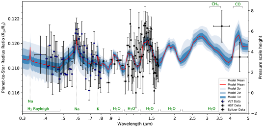
Figure 3: Comparison of the VLT, HST and Spitzer measured transmission spectra of WASP-96b (dots with $1\sigma$ vertical error bars; the bin widths are indicated with horizontal bars) with the best-fit model from the retrieval analysis (red line) with resolution identical to the data, with the $1\sigma$, $2\sigma$ and $3\sigma$ confidence levels (dark to pale blue regions).

Table 2: System parameters from HST WFC3

Parameter, symbol, unit	Value
Orbital Period, $P$, (day)	3.4252602 (fixed)
eccentricity, $e$	0 (fixed)
inclination, $i,(^{\circ})$	$85.14$ (fixed)
$a/R_{\ast}$	$8.84$ (fixed)
$HST\,G102$	$0.8-1.15\mu$m
Mid-transit time, ${\rm{T_{mid}}}$, JD	$2458470.7795^{+0.0037}_{-0.0015}$
Planet-to-star radius ratio, $\mathrm{R_{\rm{p}}/R_{\ast}}$	$0.1186^{+0.0015}_{-0.0013}$
First limb darkening coefficient, $c_{1}$	$0.631621$ (fixed)
Second limb darkening coefficient, $c_{2}$	$-0.251583$ (fixed)
Third limb darkening coefficient, $c_{3}$	$0.417851$ (fixed)
Fourth limb darkening coefficient, $c_{4}$	$-0.190682$ (fixed)
Characteristic amplitude, $A$ (ppm)	$2226^{+5369}_{-991}$
Characteristic length scale, $\eta_{\phi}$	$4\pm{3}$
Characteristic length scale, $\eta_{x}$	$7^{+4}_{-5}$
Characteristic length scale, $\eta_{y}$	$2^{+5}_{-2}$
Intercept, $a_{0}$	$0.9995^{+0.0016}_{-0.0018}$
Slope, $a_{1}$	$0.00049^{+0.00048}_{-0.00034}$
Re-scaled uncertainty, $\sigma_{w}$, (ppm)	$158^{+78}_{-64}$
$HST\,G141$	$1.075-1.700\mu$m
Mid-transit time,${\rm{T_{mid}}}$ JD	$2458481.05626^{+0.00041}_{-0.00046}$
Planet-to-star radius ratio, $R_{\rm{p}}/R_{\ast}$	$0.11962^{+0.00029}_{-0.00037}$
First limb darkening coefficient, $c_{1}$	$0.657415$ (fixed)
Second limb darkening coefficient, $c_{2}$	$-0.105797$ (fixed)
Third limb darkening coefficient, $c_{3}$	$0.031906$ (fixed)
Fourth limb darkening coefficient, $c_{4}$	$-0.019303$ (fixed)
Characteristic amplitude, $A$ (ppm), $A$ (ppm)	$2038^{+3167}_{-1156}$
Characteristic length scale, $\eta_{\phi}$	$4\pm 2$
Characteristic length scale, $\eta_{x}$	$8\pm 4$
Characteristic length scale, $\eta_{y}$	$4\pm 2$
Intercept, $a_{0}$	$0.9994\pm 0.002$
Slope, $a_{1}$	$0.00012^{+0.00028}_{-0.00025}$
Re-scaled uncertainty, $\sigma_{w}$, (ppm)	$128\pm 24$

2.4 ASSASN phase curve photometry

WASP-96 was monitored for photometric variability by the Ohio State University’s All-sky Automated Survey for Supernovae (ASAS-SN) Photometry Database, Shappee et al. (2014); Jayasinghe et al. (2019). A total of 233 photometric measurements were collected and processed during five consecutive observing campaigns starting on May 12, 2014 and ending on September 24, 2018. Each campaign, except the last one, covers the full visibility window of WASP-96 from May to January.

2.5 ESO/MPG 2.2 FEROS high resolution spectroscopy

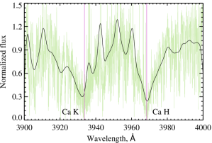
Figure 18: FEROS spectroscopy around the Ca II H&K lines for WASP-96. The green line presents the original data and the black line indicates a Gaussian smoothed version for clarity. The tabulated laboratory wavelengths of the cores of the H$\&$K lines are plotted with the purple vertical lines.

The host star of WASP-96b was observed with the MPG/ESO 2.2-metre telescope equipped with the FEROS high-resolution spectrograph (ESO program: 098.A-9007, PI P. Sarkis). Two observations with an exposure time of 900 sec were obtained on UT 2016 December 12th and 19th, using a fiber with a diameter of 2 arcsec and a spectral resolution of $R=\lambda/\delta\lambda=48,000$. The spectra were reduced with ESO’s FEROS pipeline to phase three products i.e., extracted one-dimensional spectra with wavelength solution. Both spectra have a signal-to-noise ratio of 27 over a wavelength bin of $0.03\AA$. A magnified view centered on the Ca II H&K lines from the combined spectra is shown in Figure 18.

3 Light curve analysis

Our light curve analysis of the HST, Spitzer and TESS data follows the methods detailed in Nikolov et al. (2015, 2018b, 2021).

3.1 HST WFC3 spectrophotometry

3.1.1 White-light curves

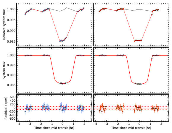
Figure 12: HST WFC3 white light curves. Left and right panels show the G102 (blue) and G141 (red) observations, respectively. The top row shows normalized raw light curves along with the marginalized Gaussian process model, assuming Matern $3/2$ kernel (grey). The later has been used as a common mode (wavelength invariant) correction for the spectroscopic light curves. The second row shows the detrended light curves along with the best-fit transit model (red). The third row shows the best-fit light curve residuals and $1\sigma$ error bars, obtained by taking the difference of the raw flux and marginalized transit and systematics models. The dashed lines indicate the light curve dispersion, $\sim 75$ parts per million.

We produced white-light curves by summing the flux of each spectrum from 0.78 to 1.13 and from 1.12 to 1.65$\mu$m for the G102 and G141 transit time series, respectively (Figure 12). Both data sets exhibit the well-known “hook” systematic, that correlates with the HST orbital phase and is considered to originate from charge-trapping in the WFC3 detector (Deming et al., 2013; Huitson et al., 2013; Zhou et al., 2017). The out-of-transit flux also exhibits a longer term drift, which is approximately linear in time.

We fit the transit and systematic effects of the white-light curves by treating the data as a Gaussian process (Gibson et al., 2012). The transit parameters: orbital period, eccentricity, inclination $i$ and normalized semi-major axis $a/R_{\ast}$ (where $R_{\ast}$ is the radius of the star) were held fixed to the previously determined values of Anderson et al. (2014) and Nikolov et al. (2018c), which are detailed in Table 2. We accounted for the stellar limb darkening by adopting the four-parameter non-linear limb-darkening law (Claret, 2000) and computed the values of the coefficients ($c_{1}$, $c_{2}$, $c_{3}$, $c_{4}$) using a three-dimensional stellar atmosphere grid (Magic et al., 2015). In these calculations, we adopted the closest match to the effective temperature, surface gravity and metallicity of the exoplanet host star found in Hellier et al. (2014). The mid-time $T_{\rm{mid}}$ and planet-to-star radius ratio ${\mathrm{R_{p}/R_{\ast}}}$ were allowed to vary in the fit to each of the two white-light curves.

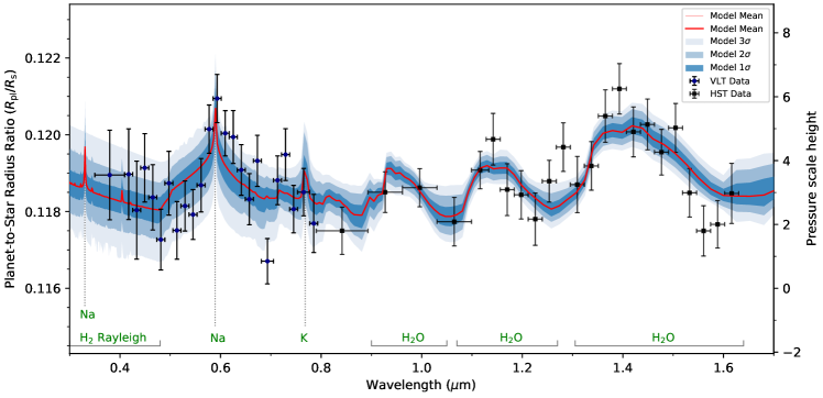
Figure 4: Same as Figure 3 but showing a zoom around the combined optical-infrared spectrum from VLT and HST. We binned with the weighted mean the VLT, G102 and G141 spectra in 2, 2 and 4 points, respectively.

Under the Gaussian process assumption, the data likelihood is a multivariate normal distribution with a mean function $\mu$ describing the deterministic transit signal and a covariance matrix $K$ that accounts for stochastic correlations (i.e., poorly constrained systematics) in the light curves:

$$p(\bm{f}|\bm{\theta},\gamma)=\mathcal{N}(\mu,K),$$ (1)

where $p$ is the probability density function, $\bm{f}$ and $\bm{\theta}$ are vectors containing the flux measurements and mean function parameters, respectively; $\gamma$ is a function containing the covariance parameters and $\mathcal{N}$ is a multivariate normal distribution. The mean function $\mu$ is defined as:

$$\mu(\bm{t},\bm{\hat{t}};a_{0},a_{1},\bm{\theta})=[a_{0}+a_{1}\bm{\hat{t}}]\,T(\bm{\emph{t}},\bm{\theta}),$$ (2)

where $\bm{t}$ is a vector of all central exposure time stamps in Julian Date, $\bm{\hat{t}}$ is a vector containing all standardized times, that is, with subtracted mean exposure time and divided by the standard deviation, $a_{0}$ and $a_{1}$ describe a linear baseline trend, $T(\bm{\theta})$ is an analytical expression describing the transit and $\bm{\theta}=(i,a/R_{\ast},T_{\rm{mid}},R_{p}/R_{\ast},c_{1},c_{2},c_{3},c_{4})$. We made use of the analytical formulae of Mandel & Agol (2002); Kreidberg (2015).

Similar to our earlier HST and VLT studies, we defined the covariance matrix as $K=\sigma_{i}^{2}\delta_{ij}+k_{ij}$, where $\sigma_{i}$ contains the photon noise uncertainties, $\delta_{ij}$ is the Kronecker delta function and $k_{ij}$ is a covariance function. The white noise term $\sigma_{w}$ was assumed to have the same value for all data points and was allowed to freely vary. We chose to use the Matérn $\nu=3/2$ kernel with the HST orbital phase ($\phi$) and spectral dispersion $(x)$ and cross-dispersion $(y)$ drifts, respectively as input variables. Our kernel choice is motivated by the study of Gibson et al. (2013), where the Matérn $\nu=3/2$ kernel is empirically motivated using simulated data, and is the first to use this kernel for light curve analysis. The GP free parameters were the characteristic correlation amplitude $(A)$ and correlation length scales for each input parameter $(\tau_{\phi},\tau_{x},\tau_{y})$. Similar to our previous studies, we also accounted for the long-term out-of-transit baseline trend with a linear time term. As with the linear time term, we also standardized the input parameters before the light curve fitting. The covariance function was defined as:

$$k_{ij}=A^{2}(1+\sqrt{3}D_{ij})\exp{-\sqrt{3}D_{ij}},$$ (3)

where $A$ is the characteristic correlation amplitude and

$$D_{ij}=\sqrt{\frac{(\bm{\hat{\phi}}_{i}-\bm{\hat{\phi}}_{j})^{2}}{\tau_{\phi}^{2}}+\frac{(\bm{\hat{x}}_{i}-\bm{\hat{x}}_{j})^{2}}{\tau_{x}^{2}}+\frac{(\bm{\hat{y}}_{i}-\bm{\hat{y}}_{j})^{2}}{\tau_{y}^{2}}},$$ (4)

where $\tau_{\phi},\tau_{x},\tau_{y}$ are the correlation length scale and the hatted variables are standardized. The parameters $\bm{X}=(a_{0},a_{1},T_{\rm{mid}},R_{p}/R_{\ast},\sigma_{w})$ and $\bm{Y}=(A,\tau_{\phi},\tau_{x},\tau_{y})$ were allowed to vary and fixed the orbital period $P$ and eccentricity $e$ to the values reported in Hellier et al. (2014) and the system parameters $(i)$ and $(a/R_{\ast})$ to the values found in Nikolov et al. (2018c).Our choice to fix the two system parameters was determined by the fact that both HST observations lack data points (except one for the last orbit of the G141 visit, Figure 12) obtained during ingress and egress. We adopted uniform priors for $x$ and log-uniform priors for $y$. We marginalize the posterior distribution by making use of the Markov-Chain Monte Carlo (MCMC) software package emcee (Foreman-Mackey et al., 2013). We identified the maximum likelihood solution using the Levenberg–Marquardt least-squares algorithm (Markwardt, 2009) and initialized three groups of $250$ walkers close to that maximum. The first two groups were run for $450$ samples and the third one for $3,500$ samples. To ensure faster convergence, we re-sampled the positions of the walkers in a narrow space around the position of the best walker from the first run before running for the second group. This helps prevent some of the walkers starting in a low-likelihood area of parameter space, which can require more computational time to converge. Figure 12 and Table 2 show transit models for each of the two observations computed using the marginalized posterior distributions and the fitted parameters, respectively. We find residual dispersion of 83 and 94 parts-per-million for the blue (G102) and red (G141) light curves, respectively.

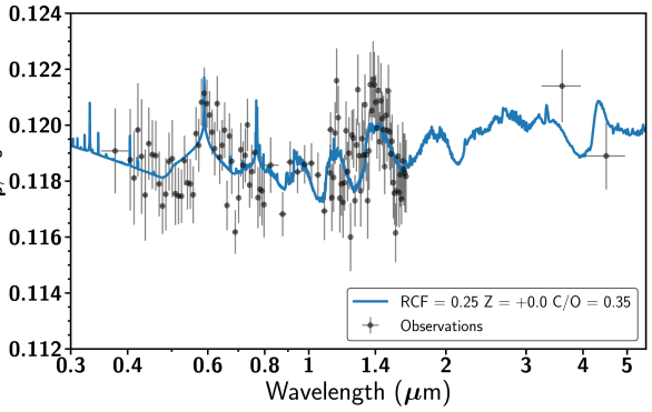
Figure 5: Comparison of the VLT, HST and Spitzer measured transmission spectrum (black dots with 1$\sigma$ error bars) with the best fit forward model transmission spectrum (blue) from the self-consistent planet-specific grid of WASP-96b across a range of re-circulation factor (RCF), metallicity (Z) and C/O ratio. $\chi^{2}=129.3$ for the best fit model spectrum. The best fit model parameters are RCF = 0.25, solar metallicity and C/O ratio of 0.35.

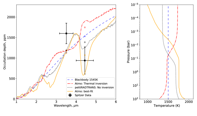
Figure 6: Emission spectrum of WASP-96b, synthetic emission spectra and assumed pressure-temperature profiles. Left panel: WASP-96b thermal spectrum from Spitzer IRAC 3.6 and 4.5 $\mu$m observations (black symbols with $1\sigma$ error bars) compared to forward synthetic spectra assuming an isothermal (dashed line), ATMO and petitRADTRANS decreasing (continuous and dotted lines, respectively) and inverted (dash-dotted line) pressure-temperature profiles. Model predictions, averaged over the wavelengths for each channel are indicated with the open symbols and color coded to the relevant model. The lowest chi-square spectrum corresponds to the ATMO synthetic spectrum, assuming a non-inverted pressure-temperature profile (continuous line). Given the relatively low level of irradiation for WASP-96b, an inverted temperature profile is rather unlikely. Yet, we include a spectrum for the inverted P-T profile merely for reference purposes, not expecting it to fit the data. Right panel: Pressure-temperature profiles assumed in the calculation of the thermal emission spectra.

3.1.2 Spectroscopic light curve analyses

We produced spectroscopic light curves by summing the flux of WASP-96 in bands with variable widths in the range from 0.7903 to 1.6396$\mu$m. Our choice for the bin widths was governed by the goal to obtain the highest spectral resolution with spectrophotometric precision that is comparable to the precision of the VLT data. We produced 9 and 56 bins for the G102 and G141 grisms, respectively. The G102 and G141 grisms overlap in wavelength over a narrow region from 1.0195 to 1.1333$\mu$m, which allows a direct comparison of the measured transit depths, Figure 3 and 4, Table 4.

We established wavelength-independent i.e., common-mode, systematic correction factors for each data set, similar to our VLT and HST studies detailed in Nikolov et al. (2014, 2016). We obtained the correction factors by dividing the white-light curve from each visit by the transit model computed with the parameters detailed in Table 2. The common-mode factors for each visit are shown in Figure 12.

We fit the spectroscopic light curves using a two-component function that takes into account the transit signal and systematics simultaneously, similar to our studies in Nikolov et al. (2016, 2018c). Prior to fitting for the systematics, we removed the common mode factors from each set of spectroscopic light curves by dividing the raw flux of the spectroscopic light curves by the corresponding common-mode factors for the relevant visit. We computed transit models using the analytical models of Mandel & Agol (2002). In the fits, we allowed only the planet-to-star radius ratio $R_{p}/R_{\ast}$ to vary. We held the four coefficients of the nonlinear limb darkening law to their theoretical values. We obtained these values following the same method as for the white light curves.

We accounted for the systematics using a fourth-order polynomial of HST orbital phase ($\phi$) and up to a second order-polynomial of dispersion and cross-dispersion drift, Figure 11. We produced all possible combinations of systematics models and performed separate fits with each of them included in the two-component function. This approach has been preferred as opposed to GP regression, as the CM-corrected HST spectroscopic light curves exhibit a lower level of systematic effects (Sing et al., 2015, 2016; Nikolov et al., 2018b). We computed the Akaike Information Criterion (AIC) for each fit and estimated the statistical weight of the model depending on the number of degrees of freedom, (Akaike 1974). We marginalized the resulting relative radii following Gibson (2014). The highest evidence models included a fourth order polynomial of HST orbital phase.

3.2 Spitzer IRAC photometry

Our light curve analysis of the 3.6 and $4.5\mu$m IRAC transits and eclipses is similar to the approach for the WFC 3 spectroscopic light curves and our previous Spitzer studies (Nikolov et al., 2015; Sing et al., 2016). We analysed the primary/secondary eclipses and instrumental systematics simultaneously. We used the analytic formulae of Mandel & Agol (2002) to fit the transit light curves and assumed the non-linear limb darkening law with coefficients computed from the three-dimensional stellar atmosphere model grid of Magic et al. (2015). To obtain an analytical eclipse model, we relied on the same formulae, but computed model with limb darkening set to zero. We fixed the remaining system parameters to literature values listed in Table 2 and fitted only for the eclipse depth and central time. To correct for the intrapixel sensitivity-induced flux variations we fit a polynomial function of the stellar centroid position of the form:

$$f(t)=a_{0}+a_{1}x+a_{2}x^{2}+a_{3}y+a_{4}y^{2}+a_{5}xy+a_{6}t,$$ (5)

where $f(t)$ is the stellar flux as a function of time, $t$; $x$ and $y$ are the positions of the stellar centroid on the detector and $a_{0}$ to $a_{6}$ are the free parameters of the fit. We produced all possible combinations of terms from Equation 5 and performed separate fits. Using the AIC statistic, we marginalized the models to obtain parameters with uncertainties following Gibson (2014).

3.2.1 Primary transits

First, we fit the Spitzer transit light curve with the goal to measure the planet system parameters. We allowed the planet orbital inclination, $i$, normalized semi-major axis, $a/R_{\ast}$, planet-to-star radius ratio, $R_{p}/R_{\ast}$ and central transit time, $T_{0}$ to vary free in the fit. The planet orbital period and eccentricity were fixed to the values reported in Table 2 and the four limb darkening coefficients were held fixed for the $3.6\mu$m and $4.5\mu$m as follows: $c_{1}=0.5493$, $c_{2}=-0.4770$, $c_{3}=0.4054$, $c_{4}=-0.1443$ and $c_{1}=0.5480$, $c_{2}=-0.6455$, $c_{3}=0.6196$, $c_{4}=-0.2232$ respectively. We found inclination values of $i=84.75\pm 0.75^{\circ}$ and $85.35\pm 0.41^{\circ}$ and normalized semi-major axis of $a/R_{\ast}=8.48\pm 0.71$ and $a/R_{\ast}=8.99\pm 0.42$ for the $3.6\mu$m and $4.5\mu$m transits respectively. We combine these measurements with other results to refine the system parameters and planet orbital ephemeris in Section 4.7.

To obtain measurements for the transmission spectrum, we first allowed the mid-transit time (${T_{0}}$) and planet-to-star radius ($R_{p}/R_{\ast}$) to vary and held fixed the orbital period ($P$), eccentricity($e$), inclination and scaled semi-major axis ($a/R_{\ast}$) to the values reported in Table 2. We found central transit times ${\rm T_{mid}}=2458779.05194\pm 0.00061$ and $2458785.90231\pm 0.00045$ (${\rm{BJD_{TDB}}}$) for the 3.6 and $4.5\mu$m channel, respectively. Finally, we repeated the fit allowing only the planet radius to vary and fixed the mid-transit times to their best-fit values from the first fit. Table 4 and Figure 13 summarize our results. Applying the wavelet method on the light curve residuals, as detailed in (Carter & Winn, 2009), we found white and red noise components $\sigma_{w}=0.010$ and $\sigma_{r}=0.0010$ for the $3.6\mu$m transit data, and $\sigma_{w}=0.012$ and $\sigma_{r}=0.0010$ for the $4.5\mu$m transit, respectively.

3.2.2 Secondary eclipses

First, we fit the secondary eclipses by allowing the mid-eclipse time (${T_{ecl}}$) and eclipse (or occultation) depth, $\delta_{occ}=(B_{\lambda}(T_{p})/B_{\lambda}(T_{\ast}))(R_{p}/R_{\ast})^{2}$ to vary freely. We find ${T_{ecl}(3.6)}=2458787.6139\pm 0.0033$ and ${T_{ecl}(4.5)}=2458794.4777\pm 0.0075$. An analysis of the departures of these measurements from the predicted ephemeris is presented in Section 4.7. We measure white and red noise components of $\sigma_{w}=0.010$ and $\sigma_{r}=0.003$ for the $3.6\mu$m transit data, and $\sigma_{w}=0.013$ and $\sigma_{r}=0.0013$ for the $4.5\mu$m transit, respectively.

In a second pass, we fixed the central eclipse times to these values and allowed only the occultation depths to vary in the light curve fits. We find $\delta_{occ}(3.6)=1600\pm 250$ and $\delta_{occ}(4.5)=926\pm 334$ parts-per-million (Figure 6).

3.3 TESS photometry

We performed fits to the TESS light curves using the same method as for the Spitzer light curves. We assumed the following limb darkening coefficients: $c_{1}=0.6228$, $c_{2}=-0.1870$, $c_{3}=0.4742$, $c_{4}=-0.2224$ and kept them fixed throughout the analysis. In addition, the planet orbital eccentricity and period were held fix to the values reported in Table 2. We first allowed all transit parameters to vary freely in the fit aiming to measure the system parameters. A weighted mean to the orbital inclination and normalized semi-major axis measured from the 2018 and 2020 light curves gave $i=85.11\pm 0.27^{\circ}$ and $a/R_{\ast}=8.66\pm 0.26$. These values are in excellent agreement with the VLT results, Table 2. Results for the central times are detailed in Table 6. In a second pass, we fixed the transit central times to the best-fit values and allowed only the planet-to-star radius ($R_{p}/R_{\ast}$) to vary. Combining all measured TESS radii, we find a weighted mean value of $R_{p}/R_{\ast}=0.11986\pm 0.00061$.

Table 3: Stellar elemental abundances of WASP-96

Abundance	Value
${\rm{[C/H]}}$	$+0.25\pm 0.19$
${\rm{[N/H]}}$	$+0.32\pm 0.16$
${\rm{[O/H]}}$	$+0.37\pm 0.11$
${\rm{[Na/H]}}$	$+0.31\pm 0.13$
${\rm{[K/H]}}$	$+0.27\pm 0.19$
${\rm{logA(Li)}}$	$1.69\pm 0.15$
${\rm{[Mg/H]}}$	$+0.47\pm 0.10$
${\rm{[Ca/H]}}$	$+0.18\pm 0.16$
${\rm{[Sc/H]}}$	$+0.14\pm 0.21$
${\rm{[Ti/H]}}$	$+0.18\pm 0.12$
${\rm{[V/H]}}$	$+0.22\pm 0.15$
${\rm{[Cr/H]}}$	$+0.25\pm 0.11$
${\rm{[Mn/H]}}$	$+0.49\pm 0.28$
${\rm{[Fe/H]}}$	$+0.21\pm 0.15$
${\rm{[Co/H]}}$	$+0.20\pm 0.15$
${\rm{[Ni/H]}}$	$+0.24\pm 0.15$
${\rm{[Y/H]}}$	$+0.17\pm 0.23$
${\rm{[Si/H]}}$	$+0.24\pm 0.16$
${\rm{[S/H]}}$	$+0.25\pm 0.11$

3.4 Stellar elemental abundances, chromospheric activity, photometric variability

We obtained abundances of the main atmospheric constituents of the host star using the FEROS spectra, using methods similar to those given in Doyle et al. (2013). Results from our analysis are shown in Table 3. Abundances are given with respect to the Solar abundances from Asplund et al. (2009), except for lithium which is given as logarithm of the number ratio with respect to hydrogen plus 12 (e.g. Bergemann & Serenelli 2014, p.247).

We compared the tabulated and observed wavelengths of the Ca II H&K line cores finding evidence for an offset of the K line wavelength as indicated in Figure 18. This has been observed toward other exoplanet host stars observed with FEROS, including WASP-110 and can be attributed to the relatively low signal-to-noise ratio (Nikolov et al., 2021). We measure the activity index, $S_{\rm HK}$, as estimated from the spectrum using the method described by Vaughan et al. (1978) and transformed to the $\log R^{\prime}_{\rm HK}$ system using the relations from Noyes et al. (1984). We find the star to be chromospherically quiet with ($\log{\rm{R^{{}^{\prime}}_{H\&K}}}=-5.3\pm 0.1$). This places WASP-96 among some of the most chromospherically quiet stars hosting a transiting exoplanet.

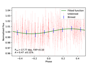
Figure 19: Phase-folded photometry from the ASAS-SN observing campaigns with the period of highest significance, as determined in our periodogram analysis. Shown are the unbinned photometry (red), binned light curve (blue), and the best-fit sine function (green). The vertical bars indicate $1\sigma$ uncertainties.

To assess the level of photometric variability due to spots on the host star, we performed Lomb-Scargle periodogram analysis on the ASAS-SN light curve with trial frequencies ranging between 0.005 and $1\,\rm{d^{-1}}$, corresponding to a period range between 1 and 200 d. We find a rotational modulation with a period of $17.8$ d with a false alarm probability (FAP) of $\sim 0.1$. We phase-folded the light curve and fitted four-parameter sine wave to measure the amplitude of the flux variation. We found an amplitude of $0.49\pm 0.11\%$ and residual scatter of 11 parts-per-thousand (ppt), Figure 19. This amplitude exceeds the $<1$mmag ($95\%$), or $<0.1\%$, rotational modulation reported by Hellier et al. (2014) by a factor of $\sim 5$. However, given the low value for chromospheric activity index in combination with the low photometric variability from the WASP photometry we conclude that the ASAS-SN result should be taken with a low weight. The TESS SAP PDC corrected light curves from sectors 2 and 29 have an average scatter of 3.4 ppt. They were examined using period04 (Lenz & Breger, 2005). No variations above 0.3 ppt were found at periods longer than the orbital period of the system. Therefore, these data confirm the lack of variation found in the WASP photometer and rule out the variation suggested by the ASAS-NS data.

4 Results and interpretation

4.1 HST-Spitzer transmission spectrum

The measured HST and Spitzer wavelength-dependent relative planet radii, which comprise the planet’s transmission spectrum are shown in Figure 1. The HST spectrum exhibits the full absorption signature of the rotational-vibrational absorption band of water with peaks at $\sim 0.95$, $1.15$ and $1.4\mu$m covering $\sim 7$ atmospheric pressure scale heights (with 1 scale height corresponding to $\sim 610$ km, assuming an equilibrium temperature of $T_{{\rm{eq}}}=1285$ K, surface gravity of $g=7.6\,\mathrm{m/s^{2}}$ and solar mean molecular weight of $\mu=2.3$ a.m.u.), in a wavelength region from $\sim 0.8$ to $1.7\mu$m.

4.2 Combining VLT with HST and Spitzer transmission spectroscopy

Following the ultimate goal of the present study i.e., extending the optical ground-based transmission spectrum of WASP-96b to infrared wavelengths, we complemented the VLT spectrum with the HST-Spitzer transit observations analyzed here. Figure 2 shows the combined ground-based and space-based spectra, presented in Nikolov et al. (2018c) and in this work, respectively. The infrared spectrum is found to be at a substantially larger radius of $\Delta R_{{\rm p}}/R_{\ast}\sim 0.004$, or a change of transit depth of $\sim 0.1\%$ ($1000$ ppm). Factors with the potential to contribute to such spectral offsets include: 1) stellar activity and photometric variability of the host star; 2) discrepancy in the system parameters assumed in the light curve fits of the separate data sets; 3) accurate accounting of the limb-darkening; 4) unaccounted systematic errors in the light curve analysis. The $<0.1\%$ photometric variability of the host star reported by Hellier et al. (2014), or even the higher variability of $0.49\pm 0.11\%$ tentatively seen in the ASAS-SN monitoring, can only account for a negligible radius offset. In this study, we assumed identical system parameters for each of the data set and the limb darkening was properly treated in both studies. We note that the limb darkening of the host star is predicted to substantially vary from optical to infrared wavelengths. The VLT data have been fit with a quadratic limb darkening law with the first coefficient allowed to vary to account for the variable transmission of the Earth atmosphere. In this study we fixed the limb darkening coefficients to their theoretical values from the same synthetic spectra assumed for the limb darkening of the ground-based data (Magic et al., 2015). A visual inspection of the light curve fits shown in Extended Data Figures 2 & 3 of Nikolov et al. (2018c) show no evidence for significant unaccounted systematics. However in that study (and here too), the authors performed a common mode correction, which strongly depends on the assumption for system parameters and particularly on the planet-to-star radius measurement. Nikolov et al. (2018c) measured planet-to-star radii of $R_{{\rm p}}/R_{\ast}=0.1147\pm 0.0014$ and $0.1168^{+0.0015}_{-0.0014}$ for the GRIS600B and GRIS600RI white light curves, respectively. While these values differ by only $\Delta R_{{\rm p}}/R_{\ast}=0.0021\pm 0.0021$, the choice for either of them displaces the mean radius of the transmission spectrum by a substantial margin. The authors chose to rely on the blue (GRIS600B) transmission spectrum, which is less affected by telluric lines, and made use of the overlapping region of the two grisms to offset the red (GRIS600RI) transmission spectrum to the inherent for the blue (GRIS600RI) spectrum smaller planet radii. Choosing the red spectrum as a reference would account for $50\%$ of the difference between the HST and VLT spectra. While Yip et al. (2021) concluded that combining datasets is risky and could not ascertain if the VLT and HST data were compatible, we point out that techniques such as common-mode corrections are well known to compromise the absolute transit depths, such that an overall transmission spectrum can have a large vertical uncertainty which is not fully captured by the point-to-point uncertainties of the relative transit depths (typically the quantity of interest). This is largely because the common-mode correction effectively assumes a broadband $R_{{\rm p}}/R_{\ast}$ with no uncertainty, which ignores the actual uncertainty on the broadband $R_{{\rm p}}/R_{\ast}$ from the white light curve fit.

With a TESS measurement from a broad-band covering the wavelength region from 0.6 to $1\mu$m, one could employ this radius to offset the VLT spectrum. However, the TESS band is centered in the small overlapping region of the red (GRIS600RI) VLT and blue HST (G102) data, which hampers quantifying the size of the offset. We also constructed a band in the HST G102 data corresponding to the narrow overlapping region with the VLT data. However, we found that the uncertainty of such a narrow band of only 3nm is insufficient to derive an accurate radius. Instead, we derive an offset correction for the VLT data by a simultaneous retrieval of the VLT and HST-Spitzer spectra as detailed in the next section.

Table 4: WASP-96b VLT, HST and Spitzer transmission spectrum after a correction of the VLT spectrum

$\mathrm{\lambda_{c}}$, $\mathrm{\mu}$m	$\mathrm{\Delta\lambda,\mu}$m	$\mathrm{R_{p}/R_{s}}$	$\mathrm{\sigma_{R_{p}/R_{s}}}$		$\mathrm{\lambda_{c}}$, $\mathrm{\mu}$m	$\mathrm{\Delta\lambda,\mu}$m	$\mathrm{R_{p}/R_{s}}$	$\mathrm{\sigma_{R_{p}/R_{s}}}$
0.37565	0.02565	0.11908	0.00152		1.12345	0.00465	0.11741	0.00120
0.40530	0.00400	0.11876	0.00182		1.13275	0.00465	0.11813	0.00124
0.41330	0.00400	0.11811	0.00167		1.14205	0.00465	0.11972	0.00111
0.42130	0.00400	0.11983	0.00167		1.15135	0.00465	0.12159	0.00116
0.42930	0.00400	0.11888	0.00205		1.16065	0.00465	0.12027	0.00114
0.43730	0.00400	0.11750	0.00163		1.16995	0.00465	0.11739	0.00123
0.44530	0.00400	0.11934	0.00129		1.17925	0.00465	0.11790	0.00114
0.45330	0.00400	0.11895	0.00123		1.18855	0.00465	0.11724	0.00127
0.46130	0.00400	0.11891	0.00125		1.19785	0.00465	0.11794	0.00100
0.46930	0.00400	0.11790	0.00116		1.20715	0.00465	0.11980	0.00105
0.47730	0.00400	0.11711	0.00100		1.21645	0.00465	0.11834	0.00106
0.48530	0.00400	0.11753	0.00130		1.22575	0.00465	0.11900	0.00129
0.49330	0.00400	0.11870	0.00104		1.23505	0.00465	0.11600	0.00122
0.50130	0.00400	0.11880	0.00138		1.24435	0.00465	0.11965	0.00088
0.50930	0.00400	0.11755	0.00112		1.25365	0.00465	0.11953	0.00105
0.51730	0.00400	0.11747	0.00101		1.26295	0.00465	0.11730	0.00092
0.52530	0.00400	0.11746	0.00096		1.27225	0.00465	0.11929	0.00095
0.53330	0.00400	0.11873	0.00089		1.28155	0.00465	0.12127	0.00126
0.54130	0.00400	0.11794	0.00095		1.29085	0.00465	0.11891	0.00117
0.54930	0.00400	0.11790	0.00089		1.30015	0.00465	0.11765	0.00128
0.55730	0.00400	0.11751	0.00102		1.30945	0.00465	0.11952	0.00129
0.56530	0.00400	0.11970	0.00095		1.31875	0.00465	0.11893	0.00124
0.57330	0.00400	0.11928	0.00095		1.32805	0.00465	0.12073	0.00109
0.58130	0.00400	0.12082	0.00084		1.33735	0.00465	0.11894	0.00094
0.58930	0.00400	0.12114	0.00092		1.34665	0.00465	0.11730	0.00136
0.59730	0.00400	0.12077	0.00086		1.35595	0.00465	0.11908	0.00139
0.60530	0.00400	0.12036	0.00086		1.36525	0.00465	0.12145	0.00117
0.61330	0.00400	0.11975	0.00081		1.37455	0.00465	0.12052	0.00106
0.62130	0.00400	0.11916	0.00096		1.38385	0.00465	0.12164	0.00136
0.62930	0.00400	0.12077	0.00099		1.39315	0.00465	0.12144	0.00118
0.63730	0.00400	0.11886	0.00096		1.40245	0.00465	0.12082	0.00097
0.64530	0.00400	0.11928	0.00091		1.41175	0.00465	0.11989	0.00109
0.65330	0.00400	0.11982	0.00100		1.42105	0.00465	0.12124	0.00125
0.66130	0.00400	0.11713	0.00089		1.43035	0.00465	0.11941	0.00106
0.66930	0.00400	0.11961	0.00081		1.43965	0.00465	0.12087	0.00135
0.67730	0.00400	0.11871	0.00117		1.44895	0.00465	0.12023	0.00097
0.68930	0.00800	0.11618	0.00078		1.45825	0.00465	0.11984	0.00122
0.70130	0.00400	0.11740	0.00090		1.46755	0.00465	0.11852	0.00099
0.70930	0.00400	0.11912	0.00096		1.47685	0.00465	0.12035	0.00099
0.71730	0.00400	0.11857	0.00085		1.48615	0.00465	0.11982	0.00113
0.72530	0.00400	0.11892	0.00097		1.49545	0.00465	0.12122	0.00094
0.73330	0.00400	0.12001	0.00094		1.50475	0.00465	0.11976	0.00136
0.74130	0.00400	0.11786	0.00081		1.51405	0.00465	0.11897	0.00112
0.74930	0.00400	0.11834	0.00096		1.52335	0.00465	0.11942	0.00095
0.76130	0.00800	0.11902	0.00075		1.53265	0.00465	0.11795	0.00128
0.77330	0.00400	0.11741	0.00109		1.54195	0.00465	0.11757	0.00113
0.78130	0.00400	0.11771	0.00096		1.55125	0.00465	0.11615	0.00105
0.78930	0.00400	0.11765	0.00123		1.56055	0.00465	0.11766	0.00127
0.79730	0.00400	0.11716	0.00117		1.56985	0.00465	0.11889	0.00112
0.82460	0.03430	0.11857	0.00099		1.57915	0.00465	0.11759	0.00124
0.87600	0.01710	0.11682	0.00079		1.58845	0.00465	0.11823	0.00115
0.91025	0.01715	0.11868	0.00074		1.59775	0.00465	0.11736	0.00091
0.94455	0.01715	0.11833	0.00076		1.60705	0.00465	0.11872	0.00139
0.97885	0.01715	0.11860	0.00069		1.61635	0.00465	0.11842	0.00129
1.01320	0.01720	0.11864	0.00072		1.62565	0.00465	0.11829	0.00140
1.04755	0.01715	0.11822	0.00080		1.63495	0.00465	0.11817	0.00130
1.08185	0.01715	0.11693	0.00104		3.60000	0.35460	0.12140	0.00130
1.11415	0.00465	0.11829	0.00101		4.50000	0.45020	0.11890	0.00120
1.11615	0.01715	0.11984	0.00063

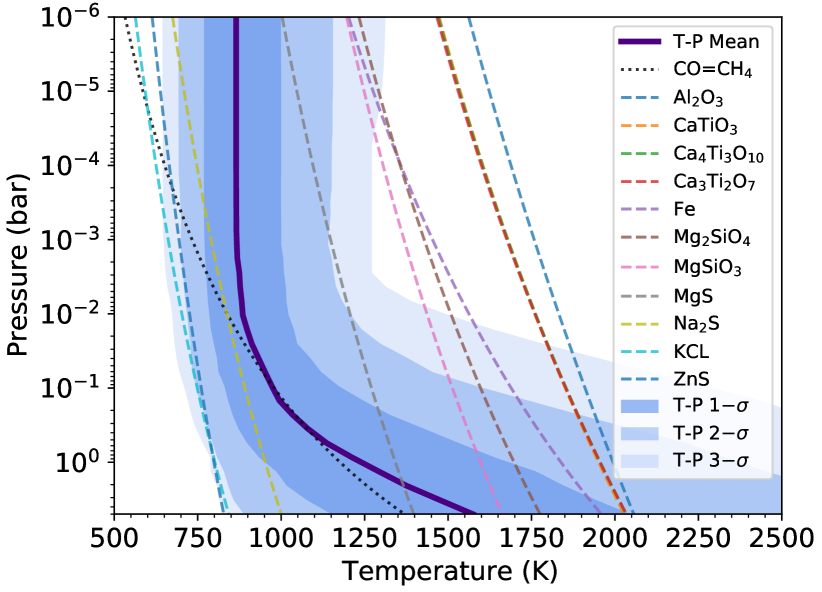
Figure 7: Pressure-temperature profile results from ATMO assuming chemical equilibrium. Shown are the median profile of the posterior distribution (purple line) and the $1\sigma$, $2\sigma$ and $3\sigma$ model distributions with dark, medium and light blue shaded regions, respectively. Cloud condensation curves, assuming solar abundance are indicated with the dashed lines from Visscher et al. 2006, 2010; Wakeford et al. 2017b.

4.3 Retrieval of the combined VLT, HST and Spitzer transmission spectrum

We considered inverse methods to constrain atmospheric properties at the day-night terminator of WASP-96b and the radius difference between the VLT optical and HST-Spitzer infrared transmission spectra. We employed the 1D-2D radiative-convective equilibrium ATMO model (Tremblin et al., 2015, 2016). Previous retrieval results using ATMO can be found in Wakeford et al. (2017a); Evans et al. (2017); Mikal-Evans et al. (2019, 2020); Spake et al. (2021); Evans et al. (2018). ATMO is capable of solving for the pressure-temperature (P-T) profile and chemical abundances that satisfy hydrostatic equilibrium and conservation of energy given a set of opacities. The code computes isotropic multi-gas Rayleigh scattering, H${}_{2}-$H₂ and H${}_{2}-$He collision-induced absorption, as well as opacities for all major chemical species taken from the most up-to-date high-temperature line list sources, including Na, K, Li, Rb, Cs, H₂, He, H₂O, CO₂, CO, CH₄ (Sauval & Tatum, 1984; Heiter et al., 2008; Barber et al., 2006; Tashkun & Perevalov, 2011; Rothman et al., 2010; Yurchenko & Tennyson, 2014; Tremblin et al., 2015, 2016; Amundsen et al., 2014, 2017; Drummond et al., 2016; Goyal et al., 2017). Rainout of condensate species is also included (see discussion in Goyal et al. 2019). ATMO can also fit a parameterized P-T profile and chemical abundances to transmission spectra. For the retrieval analysis in our study, we made use of the parameterized P-T profile detailed in Guillot (2010), which gives three free parameters: the Planck mean thermal infrared opacity ($\kappa_{\mathrm{IR}}$); the ratio of optical to infrared opacities ($\gamma_{\mathrm{O/IR}}$); and an irradiation efficiency factor ($\beta$). We set the internal temperature to $400$ K based on Thorngren et al. (2019).

ATMO treats hazes as parameterized enhanced Rayleigh scattering and clouds are assumed to add grey opacity. The code makes use of the correlated-k approximation with the random overlap method to compute the total gaseous mixture opacity, which has been shown to agree well with a full line-by-line treatment (Amundsen et al., 2017).

We first performed a retrieval assuming chemical equilibrium and allowed the radius, opacity from clouds and hazes and elemental abundances of Na, K, C and O allowed to freely vary. In the synthetic spectra, alkali line-wing shapes were computed assuming the predictions from Allard et al. (2012). We allowed four elemental abundances to vary independently, as they are major species that are also likely to be sensitive to spectral features in the data, while the rest were varied by a trace metallicity parameter $\log{(Z_{\mathrm{trace}}/Z_{\odot})}$. This quantity is not the overall bulk metallicity but contains the abundances for trace species not otherwise individually fit (i.e., all except H, He, Na, K, C and O). By varying the elemental abundances of Na, K, C and O separately, we allow for non-solar compositions but with chemical equilibrium imposed such that each model fit has a chemically plausible mix of molecules given the retrieved temperatures, pressures, and underlying elemental abundances. Importantly, by varying both O and C separately (rather than a single C/O value) we alleviate an important modeling assumption that can affect the retrieved C/O value (see Drummond et al., 2019). To quantify the radius difference between the VLT and HST-Spitzer spectra, we included a parameter that controls the offset of the VLT spectrum ($\delta_{\mathrm{VLT}}$) and was allowed to freely vary in the retrieval. We chose to discard the TESS radius measurement owing to its large uncertainty and broad wavelength region.

The best-fit transmission spectra are shown in Figure 3 and 4. The P-T profile is shown in Figure 7; and the posteriors of all retrieved quantities are shown in Figure 8. Our retrieval analysis finds a negligible contribution from cloud or haze opacity, which indicates that the atmosphere of WASP-96b is cloud and haze-free at the pressures being probed at the limb. This result is in agreement with the retrieval results from our VLT optical spectrum alone detailed in Nikolov et al. (2018c). We find an offset in the planet-to-star radius of $\delta_{\mathrm{VLT}}=0.0043^{+0.00031}_{-0.00037}$ (or a transit depth change of 1004 ppm), which is in agreement with the results of Yip et al. (2021).

We obtain constraints of $\mathrm{log(Na/Na_{\odot})}=1.32^{+0.36}_{-0.45}$ for the sodium abundance, $\mathrm{log(K/K_{\odot})}=-0.05^{+0.49}_{-0.39}$ for the potassium abundance, $\mathrm{log(C/C_{\odot})}=0.03^{+0.53}_{-0.45}$ for the carbon abundance, and $\mathrm{log(O/O_{\odot})}=0.88^{+0.38}_{-0.43}$ for the oxygen abundance, Table 5 and Figure 8. Sodium and Oxygen are the sole two elements for which we place definitive constraints, which correspond to solar to supersolar values with abundances relative to the solar values of $21^{+27}_{-14}$ (2.4-$\sigma$) and $7^{+11}_{-4}$ (2-$\sigma$), respectively. Our results are in agreement with the measured supersolar abundances of the host star Table 3. The best-fit model gives $\chi^{2}=120.96$ for 103 degrees of freedom. We note that the posterior distribution of the C/O ratio shown in Figure 8 has been reconstructed from the best-fit retrieved $\mathrm{log(C/C_{\odot})}$ and $\mathrm{log(O/O_{\odot})}$ abundances. This implies that the prior ranges for the C/O ratio are constructed for the $\mathrm{log(O/O_{\odot})}$ and $\mathrm{log(C/C_{\odot})}$ parameters which are fit separately. One limitation of the data and retrieval modeling is that the carbon-bearing species aren’t resolved by the Spitzer data, including CO₂, CO and CH₄. While our modeling assumes equilibrium chemistry to model the mixture of these gasses, it has previously been found the C/O ratio can vary dramatically depending on whether free chemistry or equilibrium chemistry assumed in the model (e.g., Spake et al. 2021).

Table 5: Retrieval results

Parameter, Unit	Value	Prior range
$\chi^{2}_{\mathrm{min}}$	$120.96$
$N_{\mathrm{free}}$	14
$N_{\mathrm{data}}$	117
$\log(Z_{\mathrm{trace}}/Z_{\odot})$	$-0.40^{+0.48}_{-0.25}$	$-1$ to $2$
$R_{\mathrm{pl}}$, ($R_{\mathrm{Jup}}$)	$1.2493^{+0.0039}_{-0.0036}$	$1.13$ to $1.39$
$\ln{\delta_{\mathrm{cloud}}}$	$-1.30^{+4.54}_{-3.36}$	$-10$ to $10$
$\ln{\delta_{\mathrm{haze}}}$	$-2.85^{+2.79}_{-2.90}$	$-10$ to $10$
Cloud Top, $\log_{10}{\mathrm{(bar)}}$	$-1.84^{+0.83}_{-1.53}$	$-6$ to $0.7$
$\alpha_{\mathrm{haze}}$	$2.45^{+1.13}_{-1.15}$	$0$ to $5$
$\delta_{\mathrm{VLT}}\times 10^{3}$	$4.29^{+0.31}_{-0.37}$	$0.29$ to $8.3$
$\log{\kappa_{\mathrm{IR}}}$	$-2.73^{+0.96}_{-0.93}$	$-5$ to $0.5$
$\log{\gamma_{\mathrm{O/IR}}}$	$-1.37^{+0.96}_{-1.15}$	$-4$ to $1.5$
$\beta$	$0.78^{+0.13}_{-0.09}$	$0$ to $2$
$\mathrm{\log(C/C_{\odot})}$	$0.03^{+0.53}_{-0.45}$	$-1$ to $2$
$\mathrm{\log(O/O_{\odot})}$	$0.88^{+0.38}_{-0.43}$	$-1$ to $2$
$\mathrm{\log(Na/Na_{\odot})}$	$1.32^{+0.36}_{-0.45}$	$-1$ to $2$
$\mathrm{\log(K/K_{\odot})}$	$-0.05^{+0.49}_{-0.39}$	$-1$ to $2$

In addition to the retrieval with alkali metals profile from Allard et al. (2012), we performed a second retrieval assuming Lorentzian profile from Burrows et al. (2000). Our results indicate an excellent agreement between the retrieved atmospheric properties of the two assumed profiles without a preference of one versus the other.

We also performed retrievals excluding the Spitzer data. Because little-to-no carbon species are needed to fit the transmission spectrum (with low $\mathrm{log(C/C_{\odot})}$ and resulting C/O ratio found), and the Spitzer data points have fairly large error bars, excluding the Spitzer data had little effect on the retrieved parameters. The $\mathrm{log(C/C_{\odot})}$ parameter was found to increase by about 0.1 dex when excluding the Spitzer data, but this is well within the retrieval uncertainties (0.5 dex).

The combined VLT-HST-Spitzer transmission spectrum after a correction of the VLT spectrum is detailed in Table 4.

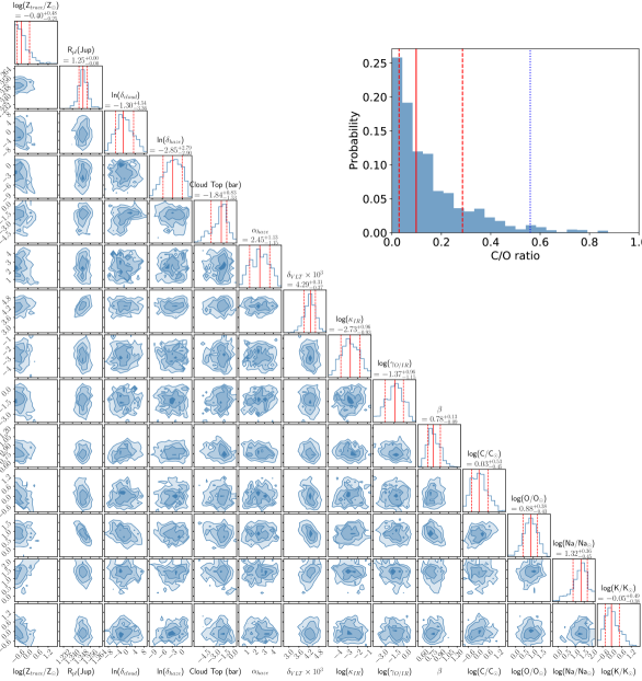
Figure 8: Atmospheric properties for WASP-96b obtained from a retrieval with ATMO, assuming chemical equilibrium. Marginalized posterior distributions of trace metallicity, planet radius, cloud and haze opacity, cloud top pressure, index of haze power, infrared opacity, optical-to-infrared offset, $\beta$ and elemental abundances of carbon, oxygen, sodium and potassium in solar units. Lack of clouds and hazes at the pressures being probed by our observations is evidenced by the high value of cloud top pressure and negligible haze opacity of the marginalized posterior distributions. The abundances of oxygen and sodium are the two constrained quantities. The mean abundances and $1\sigma$ uncertainties are indicated with the vertical continuous and dashed lines, respectively. The posterior distribution of the C/O ratio is reconstructed from the $\mathrm{\log(C/C_{\odot})}$ and $\mathrm{\log(O/O_{\odot})}$ abundances and is shown, with the solar value indicated with the blue dotted line in the top panel.

4.4 Forward Model analysis of the combined VLT, HST and Spitzer transmission spectrum

To interpret the combined WASP-96b observed transmission spectrum we also used a forward model grid of transmission spectra generated using self-consistent P-T profiles in ATMO for a range of metallicity, C/O ratio and energy re-distribution, described in detail in Goyal et al. (2020). Here, self-consistent imply radiative-convective equilibrium P-T profiles consistent with equilibrium chemical abundances. Prior to fitting the data, we offset the VLT spectrum with by $\delta=4.29$, found in the retrieval analysis. The best fit forward model transmission spectrum is shown in Figure 5. This fit corresponds to $\chi^{2}=129.3$ and reduced $\chi^{2}=1.11$ with 116 degrees of freedom (117 observed points minus 1 for the vertical offset in the transmission spectrum). This fit could be considered as a relatively good fit given that the model transmission spectrum is purely forward with self-consistent P-T profiles. The best fit transmission spectrum has a re-circulation factor of 0.25 (high energy redistribution), indicating a relatively cooler P-T profile as expected for transmission spectrum, since we probe the day-night terminator region of the exoplanet using the transmission spectrum. We also determine that the best fit forward model transmission spectrum has solar metallicity and sub-solar C/O ratio (0.35). Only one other model spectrum from the grid lie within the $1\sigma$ $\chi^{2}$ value of the best-fit transmission spectrum and this model also has solar metallicity and sub-solar C/O ratio (0.35).

4.5 Thermal emission spectrum

The two measured Spitzer IRAC eclipse depths are plotted in Figure 6 and comprise the planet’s dayside thermal spectrum. We find the 4.5$\mu$m eclipse depth to be lower compared to the $3.6\mu$m data, which suggests a decreasing temperature with altitude.

We first fit a blackbody synthetic spectrum to determine the dayside temperature of the planet. The blackbody temperature was the sole parameter allowed to freely vary in this fit. We assumed a blackbody spectrum for the host star with the effective temperature of WASP-96. We found that the best-fitting spectrum for the planet, with $\chi^{2}=6.7$ for 1 degree of freedom, and ${\rm{BIC=7.4}}$, corresponds to a temperature of $T_{\rm{p}}=1545\pm 90$ K. This spectrum corresponds to the dashed line in Figure 6.

We then employed the publicly available radiative transfer code petitRADTRANS (Mollière et al., 2019) to compute synthetic spectra for the planet’s dayside. petitRADTRANS computes planet emission spectra for an assumed pressure-temperature (P-T) profile and gravity. Because exoplanet emission spectra are known to depend on the underlying P-T profile, we chose to compute spectra, assuming P-T profiles of a decreasing (non-inverted), and an increasing (inverted) temperature with altitude. WASP-96b is irradiated rather modestly, and we wouldn’t expect to encounter an inverted temperature profile. We note that the spectrum for the inverted case is included merely for reference purposes, not expecting it to fit the data. We made use of the analytic P-T profile of Guillot (2010). We assumed solar abundances for the main atmospheric constituents, including H₂O, CO, CO₂ and CO₄ and a solar mean molecular weight of 2.33. Both spectra were computed assuming unity for the recirculation factor i.e., no redistribution of the input stellar energy in the planet’s atmosphere. Prior to comparing synthetic with observed data, we averaged the synthetic spectra within the wavelength bins of the observed spectrum and computed the corresponding $\chi^{2}$. We find the observed 3.6 and $4.5\mu$m eclipse depths to be best explained by a spectrum assuming the non-inverted profile with a chi-square of $\chi^{2}=4.6$. The spectrum assuming an inverted profile resulted in $\chi^{2}=8.8$. We note that complementary observations at a higher signal-to-noise ratio and spectral resolution would be needed to confidently confirm this result.

We also interpreted the Spitzer IRAC eclipse depths with a self-consistent planet-specific forward model grid of emission spectra as shown in Goyal et al. (2021). These emission spectra were generated using radiative-convective equilibrium P-T profiles consistent with equilibrium chemical abundances in ATMO for WASP-96b, for a range of metallicity, C/O ratio and energy re-distribution, described in detail in Goyal et al. (2020). The best fit model emission spectrum and the corresponding P-T profile is shown in Figure 6. We find the observed 3.6 and $4.5\,\mu$m eclipse depths to be best explained by a spectrum with non-inverted P-T profile with $\chi^{2}=3.8$. The best fit model emission spectrum corresponds to a re-circulation factor of 1, implying none of the energy is redistributed to the night side and therefore the P-T profile corresponding to this best fit model emission spectrum is one of the hottest in the grid of models for WASP-96b. The best fit model emission spectrum corresponds to a metallicity of 200 times solar and C/O ratio of 0.7. However, by looking at all the model spectra that lie within the $1\sigma$ $\chi^{2}$ value of the best-fit emission spectrum we determine that a large range of metallicities (From 1x to 200x solar) and C/O ratio (0.35 to 0.7) can explain observed eclipse depths due to large uncertainty in the $4.5\,\mu$m eclipse depth. Interestingly, all these model spectra similar to the best-fit model spectrum have non-inverted P-T profiles and correspond to a re-circulation factor of 1 (no-redistribution), driven by the higher $3.6\,\mu$m eclipse depths requiring higher temperatures. The strong absorption in the $4.5\,\mu$m band is a result of CO, leading to lower eclipse depth in this band as seen in left side of Figure 6 for the best fit model. Therefore, the best fit model has a non-inverted P-T profile which results in this absorption feature (instead of an inverted P-T profile that would lead to an emission feature due to CO, in the $4.5\,\mu$m band). All the model spectra that lie within the $1\sigma$ $\chi^{2}$ value of the best-fit emission spectrum show this CO absorption feature but with varying degree of strength (i.e model $4.5\,\mu$m eclipse depth).

4.6 Refined system parameters

To improve the planet orbital inclination and semi-major axis of WASP-96b, we combined our measurements with literature results. In particular, our Spitzer and TESS measurements were complemented with the VLT results reported in Nikolov et al. (2018c). Weighted mean results for the orbital inclination, $i$ and normalized semi-major axis $a/R$ are reported in Table 7. Both results agree within $2\sigma$ with the measurements of Hellier et al. (2014).

4.7 Improved planet orbital ephemeris

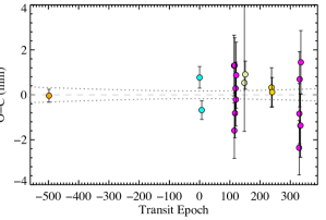
Figure 17: Observed minus computed (O-C) transit times from the best-fitting orbital period and central transit times reported in the literature (orange: combined analysis of WASP, EulerCam and TRAPPIST light curves; cyan: VLT transits) and derived from our analysis of TESS (magenta), HST (green) and Spitzer (yellow) light curves. The error bars and dotted lines indicate the $1\sigma$ uncertainties of the transit times and derived ephemeris, respectively.

We combined the central transit times from our HST, Spitzer and TESS light curve analysis with the transit times reported by Hellier et al. (2014) and Nikolov et al. (2018c) to derive an updated transit ephemeris of WASP-96b. These two studies respectively include a single transit mid-time from a combined analysis of WASP, EulerCam and TRAPPIST light curves, and central times from two VLT FORS2 white light curves. All central times were converted to BJDs (by making use of the utilities detailed in Eastman et al. 2010) and fitted with a linear function of the planet orbital period ($P$), zero-epoch central transit time ($T_{0}$) and transit epoch ($E$): $T_{\rm{C}}(E)=T_{0}+EP$. Our results for the fitted parameters are reported in Table 7 and resulted in a reduced chi-square of $\chi^{2}_{r}=1.03$ for $18$ degrees of freedom. The updated ephemeris is in an excellent agreement with the ephemeris reported by Hellier et al. (2014) and Yip et al. (2021) and does not indicate the presence of transit timing variations (TTVs). Results for the measured mid-transit times, observed minus computed transit times (O$-$C) are tabulated in Table 6 and plotted in Figure 17.

Table 6: Central transit times

Epoch	Mid-transit time, ${\rm{BJD}}_{{\rm{TDB}}}$	O$-$C, day	Data	Note
$-498$	$2456258.06290\pm{0.00020}$	$-0.000027$	WASP	$1$
$0$	$2457963.84120^{+0.00034}_{-0.00033}$	$0.000534$	VLT	$2$
$7$	$2457987.81699\pm{0.00029}$	$-0.000472$	VLT	$2$
$114$	$2458354.32081\pm{0.00094}$	$0.000902$	TESS	$3$
$115$	$2458357.74406\pm{0.00086}$	$-0.001104$	TESS	$3$
$116$	$2458361.17133\pm{0.00085}$	$0.000909$	TESS	$3$
$117$	$2458364.59511\pm{0.00076}$	$-0.000567$	TESS	$3$
$119$	$2458371.44639\pm{0.00081}$	$0.000200$	TESS	$3$
$120$	$2458374.87130\pm{0.00082}$	$-0.000147$	TESS	$3$
$121$	$2458378.29731\pm{0.00102}$	$0.000607$	TESS	$3$
$148$	$2458470.77900^{+0.00370}_{-0.00150}$	$0.000371$	HST	$3$
$151$	$2458481.05503^{+0.00041}_{-0.00046}$	$0.000632$	HST	$3$
$238$	$2458779.05194\pm{0.00061}$	$0.000226$	Spitzer	$3$
$240$	$2458785.90231\pm{0.00045}$	$0.000083$	Spitzer	$3$
$329$	$2459090.74842\pm{0.00084}$	$-0.001636$	TESS	$3$
$330$	$2459094.17473\pm{0.00093}$	$-0.000582$	TESS	$3$
$331$	$2459097.60105\pm{0.00085}$	$0.000481$	TESS	$3$
$333$	$2459104.45013\pm{0.00098}$	$-0.000952$	TESS	$3$
$334$	$2459107.87539\pm{0.00098}$	$-0.000948$	TESS	$3$
$335$	$2459111.30260\pm{0.00098}$	$0.001005$	TESS	$3$

We used the refined orbital ephemeris to predict the central times of the observed secondary eclipses. Significant departures of mid-eclipse times, measured as the difference ($\Delta t_{\mathrm{O-C}}$) between the observed and computed times would indicate a non-circular planet orbit. Table 7 summarizes the values for $\Delta t_{\mathrm{O-C}}(3.6)$ and $\Delta t_{\mathrm{O-C}}(4.5)$, which agree with the predictions at $1\sigma$ and $\sim 1.6\sigma$ and indicate no departures from a circular orbit. Finally, we used Equation (6) from Wallenquist (1950) to calculate $e\cos{\omega}$ for the two eclipses. Table 7 details the weighted mean value from the two observations.

Table 7: System parameters and orbital ephemeris

Parameter, symbol, unit	Value
inclination, $i$,$(^{\circ})$	$85.135\pm 0.081$
$a/R_{\ast}$	$8.820\pm 0.090$
Orbital Period, $P$, (day)	$3.42525650\pm 0.00000037$
Transit central time, $T_{0}$, (BJD)	$2457963.84067\pm 0.00012$
$\Delta t_{\mathrm{O-C}}(3.6)$, (min)	$-1.4\pm 4.8$
$\Delta t_{\mathrm{O-C}}(4.5)$, (min)	$18\pm 11$
$e\cos(\omega)$	$-0.00790\pm 0.00010$

5 Discussion

The sodium abundance obtained from our retrieval analysis of the combined optical-infrared transmission spectrum, ${\rm{\log(Na/Na_{\odot})}}$ = $1.32^{+0.36}_{-0.45}$, is about one order of magnitude larger, but is still compatible with the previous determination using only the VLT spectrum, $\log{\epsilon_{\mathrm{\,Na}}}=6.9^{+0.6}_{-0.4}$ i.e., ${\rm{\log(Na/Na_{\odot})}}$ = $0.66^{+0.6}_{-0.4}$ at the $\sim 1.2\sigma$ level.

5.1 A comparison with an earlier result

An analysis of the HST G102 and G141 transit spectroscopy and the Spitzer IRAC 3.6 and $4.5\mu$m photometric transits has been presented by Yip et al. (2021). We find the two spectra to be slightly offset by a mean difference between the spectrum from this work and the literature spectrum of $\mathrm{\Delta R_{p}/R_{s}}=(47.36\pm 0.24)\times 10^{-5}$, measured using the VLT wavelengths. This offset is consistent the uncertainty of $\mathrm{R_{p}/R_{s}}$ found in our analysis of the white light curve (see Table 2). After applying the mean difference, the two spectra are in a respectable agreement with regards to the spectral shape (Figure 9). The Spitzer IRAC radii are found to be in a good agreement at the $\sim 1\sigma$ confidence level. We note significantly smaller uncertainties, a factor of $\sim 2.2$ of the Spitzer radii measured in our work compared to the results of Yip et al. (2021). Factors that can contribute to such significant difference include unaccounted systematics effects or fits performed to binned light curves. Yet, we are unsure of the exact reasons. We additionally note a marginal difference in the radii of the VLT spectrum and their uncertainties reported by Yip et al. (2021). Finally, the G102 bin widths of the literature result reported in their Table 6 are a factor of ten smaller than the plotted bin widths throughout that study. We are unsure for the reason that led to this misquotation of the published results. Despite the differences between the literature transmission spectrum and the spectrum reported in this work, both studies find abundance results in excellent agreement using different analysis and retrieval methods.

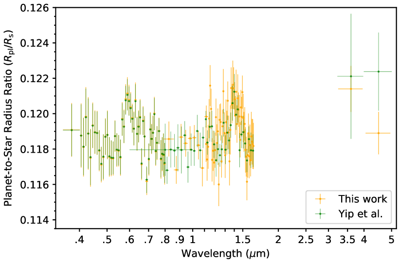
Figure 9: Comparison between the result in this work with those of Yip et al. (2021). An offset of $\mathrm{\Delta R_{p}/R_{s}}=(47.36\pm 0.24)\times 10^{-5}$ has been added to the literature result measured using the VLT spectrum. The horizontal bars represent $1\sigma$ uncertainties and the horizontal bars are the wavelength bins used to measure the transmission spectra.

5.2 Exoplanet abundances in the Solar System context

Elemental abundances of planetary atmospheres are a consequence of the joint influence of atmospheric chemical processes, formation conditions and migration (Line et al., 2021; Fortney et al., 2013; Madhusudhan, 2012; Lothringer et al., 2021). In the standard core-accretion paradigm, as they form, giant planets accrete H/He-dominated gas, as well as planetesimals that enrich their H/He envelopes in metals. Higher metal enrichment is expected for low-mass H/He envelopes, as these envelopes have smaller amount of gas for the in-falling metals to be mixed into. This is the case of the gas giants Jupiter and Saturn and the ice giants Uranus and Neptune in our own Solar System, which have elemental abundances that increase with a decreasing mass and also coincides with an increasing distance from the Sun (Figure 10, Atreya et al. 2016, 2020; Anders & Grevesse 1989; Asplund et al. 2009).

Our abundance and retrieval analysis show that both the host star and planet in the WASP-96 system have solar-to-supersolar elemental abundances of their atmospheres (Table 3 and 5). While metal enrichenment of planets does not appear to correlate with the metallicity of the parent star (Teske et al., 2019), the case of WASP-96 is a prime example for a significant enrichment of both, which likely reflects the initial formation conditions of this system. Comparing the oxygen abundance ratio for the atmosphere of WASP-96b relative to its host star, we find an oxygen ratio of $3.2\pm 0.4$, which is similar to the oxygen ratio of Jupiter’s atmosphere and the Halley’s comet in our Solar System relative to the oxygen abundance of the Sun (Anders & Grevesse, 1989). We find a higher ratio of $10^{+0.4}_{-0.5}$ for the abundance of sodium in the atmosphere of WASP-96b relative to its host star, which is in agreement with the corresponding value for the Halley’s comet relative to the Sun, which doesn’t hold for Jupiter. A recent study by Bhattacharya et al. (2021) shows evidence for alkali elements in the deep atmosphere of Jupiter from the Juno microwave data pointing toward severely subsolar values. This implies a much lower abundance ratio of sodium for the atmosphere of Jupiter compared to the solar value.

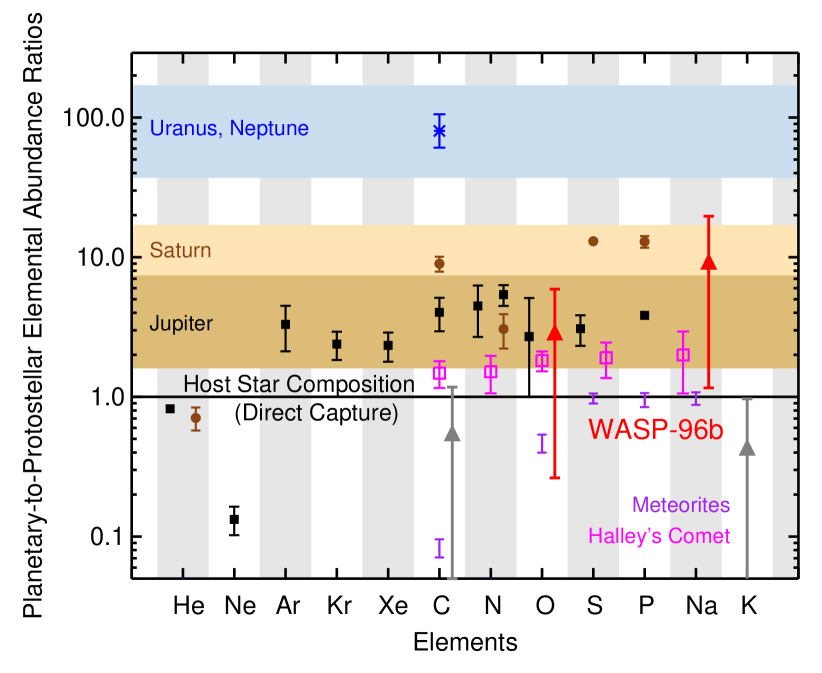
Figure 10: Elemental abundance ratios in the atmospheres of our own Solar System planets Jupiter, Saturn, Uranus and Neptune, meteorites and the Halley’s comet, relative to the protosolar values (adapted from Atreya et al. 2020). The oxygen abundance of Jupiter has been updated to the latest measurement reported by  Li et al. (2020). Elemental abundance ratios for the atmosphere of WASP-96b relative to the protstellar abundances have been obtained with the same assumption as for the protosun i.e., by increasing the protostellar value by $+0.04$  (Asplund et al., 2009). Oxygen and sodium are the only two abundances obtained for WASP-96b (red symbols) and the grey triangles indicate unbounded abundances for potassium and carbon.

6 Summary and conclusions

We presented HST WFC3 transit and Spitzer IRAC transit and eclipse observations of the atmosphere of the hot Saturn WASP-96b. This atmosphere has been identified by our team as cloud-free from a reconnaissance optical transmission spectroscopy made with the VLT. The ground-based spectrum exhibits the full pressure-broadened sodium profile, absorption from potassium and lithium and scattering from H₂ in the near-UV. Our team has motivated the HST WFC3 observations with the goal to extend the planet’s transmission spectrum at infrared wavelengths to search for the theoretically predicted absorption from H₂O, CO and CO₂, and to constrain atmospheric composition. The secondary eclipse observations were aimed at constraining the planet’s dayside temperature. The HST-Spitzer observations reveal the full absorption signature of water, which is an independent new evidence that the planet’s atmosphere is free of clouds at the terminator and at pressures being probed. Similar to earlier analysis of the HST-Spitzer transits, we find the HST-Spitzer spectrum to be at a significantly larger planet-to-star radius relative to the VLT level. We confirm and correct for a spectral offset of $\Delta R_{{\rm p}}/R_{\ast}=(-4.29^{+0.31}_{-0.37})\,\times 10^{-3}$ of the VLT data relative to the HST-Spitzer spectrum. This offset can be explained by the assumed radius and corresponding uncertainty for the common-mode correction of the VLT spectra, which is a well-known feature of ground-based transmission spectroscopy. We find evidence for a lack of chromospheric and photometric activity of the host star and therefore have an insufficient contribution to the offset. We measure abundances for Na and O that are consistent with solar-to-supersolar, with abundances relative to solar values of $21^{+27}_{-14}$ (2.4-$\sigma$) and $7^{+11}_{-4}$ (2-$\sigma$), respectively. While combining transmission spectra from space and the ground isn’t trivial, finding the first evidence for a cloudless atmosphere from the ground and the following independent confirmation from space-based observations at new, highly-complementary wavelengths, our results demonstrate the key role of ground-based low-resolution transmission spectroscopy, particularly the VLT with FORS2, in exploring the atmospheres of transiting exoplanets. A fit of a spectrum of a blackbody isothermal atmosphere to the thermal spectrum constrains a dayside brightness temperature of $T_{\rm{p}}$=$1545$$\pm$$90$K. While metal enrichenment of exoplanets has been shown not to correlate with the metallicity of their parent stars, the case of WASP-96 is a prime example for a significant enrichment of both the star and planet, which likely reflects the initial formation conditions of this system.

Data Availability

Raw and calibrated Hubble Space Telescope spectral transit time series and Spitzer Space Telescope transit and eclipse time series photometry are publicly available at the Mikulski Archive for Space Telescopes (MAST; https://archive.stsci.edu) and the NASA/IPAC Infrared Science Archive (IRSA; https://sha.ipac.caltech.edu/applications/Spitzer/SHA/), respectively. TESS light curves are publicly available at the MAST archive. Calibrated and extracted high-resolution FEROS spectra are publicly available via the European Southern Observatory’s Spectral Data Products Query Form (http://archive.eso.org/wdb/wdb/adp/phase3_spectral/form). Broad-band light curves are publicly available at the webpage of the All-Sky Automated Survey for Supernovae (ASAS-SN; https://asas-sn.osu.edu).

Appendix A Light curves and auxiliary parameters

Plots of the separate time series observations along with the complementary detrending data.

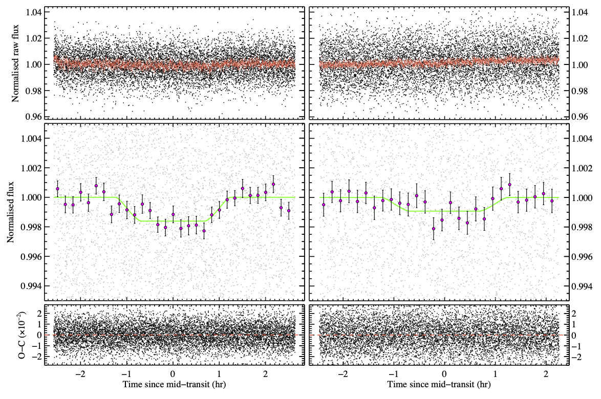
Figure 14: Spitzer  IRAC 3.6 and 4.5 $\mu$m eclipse photometry (left and right,respectively).Top panels: raw flux and the best-fitting transit and systematics model; middle panels: detrended light curves and the best-fitting eclipse models and binned by 10 min; lower panels: light-curve residuals.

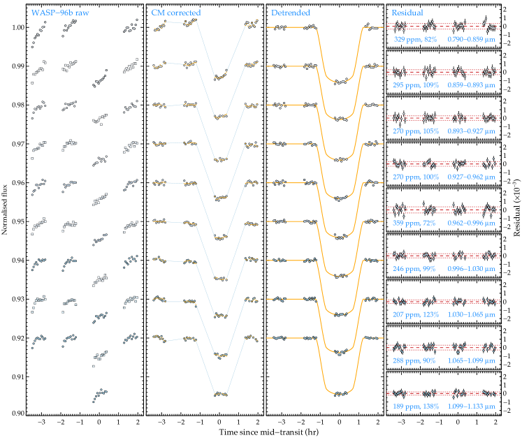
Figure 15: Spectrophotometric light curves from grism G102 offset by a constant for clarity. The first panel displays raw flux. We used dots and square symbols for the odd and even light curves, respectively to better distinguish the individual light curves. The second panel shows the common-mode (CM)-corrected light curves with transit and systematics models (lines) with the highest statistical weight. The third panel is similar to the second one, but showing the detrended light curves and transit models. The fourth panel shows residuals with $1\sigma$ uncertainties. The dashed lines indicate the median residual values, with dotted lines indicating the residual dispersion level and the percentage of the theoretical photon noise limit reached (blue) for each channel.

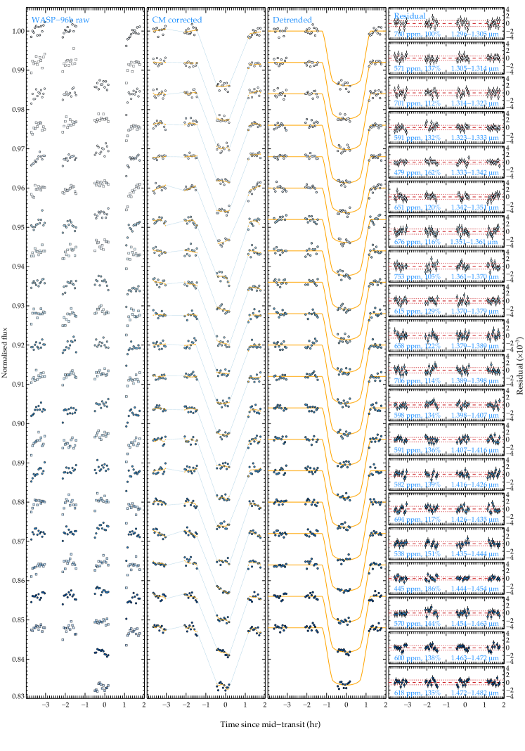
Figure 16: Same as Figure15 but for grism G141. Shown is a subset of 20 light curves.

Appendix B Stellar activity and photometric variability

This section contains figures from our analysis of the FEROS high-resolution spectroscopy and ASAS-SN light curve.

References

- Akaike (1974) Akaike H., 1974, IEEE Transactions on Automatic Control, 19, 716
- Alam et al. (2020) Alam M. K., et al., 2020, AJ, 160, 51
- Alam et al. (2021) Alam M. K., et al., 2021, ApJ, 906, L10
- Allard et al. (2012) Allard F., Homeier D., Freytag B., 2012, Philosophical Transactions of the Royal Society of London Series A, 370, 2765
- Amundsen et al. (2014) Amundsen D. S., Baraffe I., Tremblin P., Manners J., Hayek W., Mayne N. J., Acreman D. M., 2014, A&A, 564, A59
- Amundsen et al. (2017) Amundsen D. S., Tremblin P., Manners J., Baraffe I., Mayne N. J., 2017, A&A, 598, A97
- Anders & Grevesse (1989) Anders E., Grevesse N., 1989, Geochimica Cosmochimica Acta, 53, 197
- Anderson et al. (2014) Anderson D. R., et al., 2014, arXiv e-prints, p. arXiv:1410.3449
- Asplund et al. (2009) Asplund M., Grevesse N., Sauval A. J., Scott P., 2009, ARA&A, 47, 481
- Atreya et al. (2016) Atreya S. K., Crida A., Guillot T., Lunine J. I., Madhusudhan N., Mousis O., 2016, arXiv e-prints, p. arXiv:1606.04510
- Atreya et al. (2020) Atreya S. K., Hofstadter M. H., In J. H., Mousis O., Reh K., Wong M. H., 2020, Space Sci. Rev., 216, 18
- Barber et al. (2006) Barber R. J., Tennyson J., Harris G. J., Tolchenov R. N., 2006, MNRAS, 368, 1087
- Bergemann & Serenelli (2014) Bergemann M., Serenelli A., 2014, Solar Abundance Problem. pp 245–258, doi:10.1007/978-3-319-06956-2_21
- Bhattacharya et al. (2021) Bhattacharya A., Li C., Atreya S., Steffes P., Levin S., Bolton S., 2021, in AAS/Division for Planetary Sciences Meeting Abstracts. p. 212.01
- Brewer et al. (2016) Brewer J. M., Fischer D. A., Valenti J. A., Piskunov N., 2016, ApJS, 225, 32
- Burke et al. (2015) Burke C. J., et al., 2015, ApJ, 809, 8
- Burrows et al. (2000) Burrows A., Marley M. S., Sharp C. M., 2000, ApJ, 531, 438
- Caldwell et al. (2020) Caldwell D. A., et al., 2020, Research Notes of the American Astronomical Society, 4, 201
- Carter & Winn (2009) Carter J. A., Winn J. N., 2009, ApJ, 704, 51
- Carter et al. (2020) Carter A. L., et al., 2020, MNRAS, 494, 5449
- Claret (2000) Claret A., 2000, A&A, 363, 1081
- Deming et al. (2013) Deming D., et al., 2013, ApJ, 774, 95
- Doyle et al. (2013) Doyle A. P., et al., 2013, MNRAS, 428, 3164
- Drummond et al. (2016) Drummond B., Tremblin P., Baraffe I., Amundsen D. S., Mayne N. J., Venot O., Goyal J., 2016, A&A, 594, A69
- Drummond et al. (2019) Drummond B., Carter A. L., Hébrard E., Mayne N. J., Sing D. K., Evans T. M., Goyal J., 2019, MNRAS, 486, 1123
- Eastman et al. (2010) Eastman J., Siverd R., Gaudi B. S., 2010, PASP, 122, 935
- Ehrenreich et al. (2015) Ehrenreich D., et al., 2015, Nature, 522, 459
- Evans et al. (2017) Evans T. M., et al., 2017, preprint, (arXiv:1708.01076)
- Evans et al. (2018) Evans T. M., et al., 2018, AJ, 156, 283
- Fazio et al. (2004) Fazio G. G., et al., 2004, ApJS, 154, 10
- Foreman-Mackey (2015) Foreman-Mackey D., 2015, George: Gaussian Process regression, Astrophysics Source Code Library (ascl:1511.015)
- Foreman-Mackey et al. (2013) Foreman-Mackey D., Hogg D. W., Lang D., Goodman J., 2013, PASP, 125, 306
- Fortney (2005) Fortney J. J., 2005, MNRAS, 364, 649
- Fortney et al. (2010) Fortney J. J., Shabram M., Showman A. P., Lian Y., Freedman R. S., Marley M. S., Lewis N. K., 2010, ApJ, 709, 1396
- Fortney et al. (2013) Fortney J. J., Mordasini C., Nettelmann N., Kempton E. M. R., Greene T. P., Zahnle K., 2013, ApJ, 775, 80
- Fortney et al. (2021) Fortney J. J., Dawson R. I., Komacek T. D., 2021, Journal of Geophysical Research (Planets), 126, e06629
- Fu et al. (2021) Fu G., et al., 2021, AJ, 162, 108
- Gibson (2014) Gibson N. P., 2014, MNRAS, 445, 3401
- Gibson et al. (2012) Gibson N. P., Aigrain S., Roberts S., Evans T. M., Osborne M., Pont F., 2012, MNRAS, 419, 2683
- Gibson et al. (2013) Gibson N. P., Aigrain S., Barstow J. K., Evans T. M., Fletcher L. N., Irwin P. G. J., 2013, MNRAS, 436, 2974
- Gibson et al. (2017) Gibson N. P., Nikolov N., Sing D. K., Barstow J. K., Evans T. M., Kataria T., Wilson P. A., 2017, MNRAS, 467, 4591
- Goyal et al. (2017) Goyal J., et al., 2017, MNRAS, 999, X99
- Goyal et al. (2019) Goyal J. M., et al., 2019, MNRAS, 486, 783
- Goyal et al. (2020) Goyal J. M., et al., 2020, MNRAS, 498, 4680
- Goyal et al. (2021) Goyal J. M., Lewis N. K., Wakeford H. R., MacDonald R. J., Mayne N. J., 2021, ApJ, 923, 242
- Guillot (2010) Guillot T., 2010, A&A, 520, A27
- Heiter et al. (2008) Heiter U., et al., 2008, in Journal of Physics Conference Series. p. 012011, doi:10.1088/1742-6596/130/1/012011
- Hellier et al. (2014) Hellier C., et al., 2014, MNRAS, 440, 1982
- Howard et al. (2010) Howard A. W., et al., 2010, Science, 330, 653
- Howard et al. (2012) Howard A. W., et al., 2012, ApJS, 201, 15
- Huitson et al. (2013) Huitson C. M., et al., 2013, MNRAS, 434, 3252
- Jayasinghe et al. (2019) Jayasinghe T., et al., 2019, MNRAS, 485, 961
- Knutson et al. (2012) Knutson H. A., et al., 2012, ApJ, 754, 22
- Kreidberg (2015) Kreidberg L., 2015, PASP, 127, 1161
- Kurucz (1979) Kurucz R. L., 1979, ApJS, 40, 1
- Lecavelier Des Etangs et al. (2008) Lecavelier Des Etangs A., Pont F., Vidal-Madjar A., Sing D., 2008, A&A, 481, L83
- Lenz & Breger (2005) Lenz P., Breger M., 2005, Communications in Asteroseismology, 146, 53
- Li et al. (2020) Li C., et al., 2020, Nature Astronomy, 4, 609
- Line et al. (2021) Line M. R., et al., 2021, Nature, 598, 580
- Lothringer et al. (2021) Lothringer J. D., Rustamkulov Z., Sing D. K., Gibson N. P., Wilson J., Schlaufman K. C., 2021, ApJ, 914, 12
- Madhusudhan (2012) Madhusudhan N., 2012, ApJ, 758, 36
- Madhusudhan et al. (2017) Madhusudhan N., Bitsch B., Johansen A., Eriksson L., 2017, MNRAS, 469, 4102
- Magic et al. (2015) Magic Z., Weiss A., Asplund M., 2015, A&A, 573, A89
- Mandel & Agol (2002) Mandel K., Agol E., 2002, ApJ, 580, L171
- Markwardt (2009) Markwardt C. B., 2009, in Bohlender D. A., Durand D., Dowler P., eds, Astronomical Society of the Pacific Conference Series Vol. 411, Astronomical Data Analysis Software and Systems XVIII. p. 251 (arXiv:0902.2850)
- Mayor et al. (2011) Mayor M., et al., 2011, arXiv e-prints, p. arXiv:1109.2497
- Mighell (2005) Mighell K. J., 2005, MNRAS, 361, 861
- Mikal-Evans et al. (2019) Mikal-Evans T., et al., 2019, MNRAS, 488, 2222
- Mikal-Evans et al. (2020) Mikal-Evans T., Sing D. K., Kataria T., Wakeford H. R., Mayne N. J., Lewis N. K., Barstow J. K., Spake J. J., 2020, MNRAS, 496, 1638
- Mollière et al. (2019) Mollière P., Wardenier J. P., van Boekel R., Henning T., Molaverdikhani K., Snellen I. A. G., 2019, A&A, 627, A67
- Nikolov et al. (2014) Nikolov N., et al., 2014, MNRAS, 437, 46
- Nikolov et al. (2015) Nikolov N., et al., 2015, MNRAS, 447, 463
- Nikolov et al. (2016) Nikolov N., Sing D. K., Gibson N. P., Fortney J. J., Evans T. M., Barstow J. K., Kataria T., Wilson P. A., 2016, ApJ, 832, 191
- Nikolov et al. (2018a) Nikolov N., et al., 2018a, Characterizing a new prototype Saturn-mass exoplanet with the clearest atmosphere yet, HST Proposal
- Nikolov et al. (2018b) Nikolov N., et al., 2018b, MNRAS, 474, 1705
- Nikolov et al. (2018c) Nikolov N., et al., 2018c, Nature, 557, 526
- Nikolov et al. (2019) Nikolov N., Sing D., Fortney J., Deming D., Kataria T., Mayne N., Drummond B., Goyal J., 2019, Characterizing a new prototype Saturn-mass exoplanet with the clearest atmosphere yet, Spitzer Proposal
- Nikolov et al. (2021) Nikolov N., et al., 2021, AJ, 162, 88
- Noyes et al. (1984) Noyes R. W., Hartmann L. W., Baliunas S. L., Duncan D. K., Vaughan A. H., 1984, ApJ, 279, 763
- Öberg et al. (2011) Öberg K. I., Murray-Clay R., Bergin E. A., 2011, ApJ, 743, L16
- Ricker et al. (2014) Ricker G. R., et al., 2014, in Oschmann Jacobus M. J., Clampin M., Fazio G. G., MacEwen H. A., eds, Society of Photo-Optical Instrumentation Engineers (SPIE) Conference Series Vol. 9143, Space Telescopes and Instrumentation 2014: Optical, Infrared, and Millimeter Wave. p. 914320 (arXiv:1406.0151), doi:10.1117/12.2063489
- Rothman et al. (2010) Rothman L. S., et al., 2010, J. Quant. Spectrosc. Radiative Transfer, 111, 2139
- Sauval & Tatum (1984) Sauval A. J., Tatum J. B., 1984, ApJS, 56, 193
- Shappee et al. (2014) Shappee B. J., et al., 2014, ApJ, 788, 48
- Sheppard et al. (2021) Sheppard K. B., et al., 2021, AJ, 161, 51
- Sing et al. (2013) Sing D. K., et al., 2013, MNRAS, 436, 2956
- Sing et al. (2015) Sing D. K., et al., 2015, MNRAS, 446, 2428
- Sing et al. (2016) Sing D. K., et al., 2016, Nature, 529, 59
- Spake et al. (2021) Spake J. J., et al., 2021, MNRAS, 500, 4042
- Spyratos et al. (2021) Spyratos P., et al., 2021, MNRAS, 506, 2853
- Tashkun & Perevalov (2011) Tashkun S. A., Perevalov V. I., 2011, J. Quant. Spectrosc. Radiative Transfer, 112, 1403
- Teske et al. (2019) Teske J. K., Thorngren D., Fortney J. J., Hinkel N., Brewer J. M., 2019, AJ, 158, 239
- Thorngren et al. (2016) Thorngren D. P., Fortney J. J., Murray-Clay R. A., Lopez E. D., 2016, ApJ, 831, 64
- Thorngren et al. (2019) Thorngren D., Gao P., Fortney J. J., 2019, ApJ, 884, L6
- Tremblin et al. (2015) Tremblin P., Amundsen D. S., Mourier P., Baraffe I., Chabrier G., Drummond B., Homeier D., Venot O., 2015, ApJ, 804, L17
- Tremblin et al. (2016) Tremblin P., Amundsen D. S., Chabrier G., Baraffe I., Drummond B., Hinkley S., Mourier P., Venot O., 2016, ApJ, 817, L19
- Vaughan et al. (1978) Vaughan A. H., Preston G. W., Wilson O. C., 1978, PASP, 90, 267
- Visscher et al. (2006) Visscher C., Lodders K., Fegley Jr. B., 2006, ApJ, 648, 1181
- Visscher et al. (2010) Visscher C., Lodders K., Fegley Bruce J., 2010, ApJ, 716, 1060
- Wakeford et al. (2017a) Wakeford H. R., et al., 2017a, Science, 356, 628
- Wakeford et al. (2017b) Wakeford H. R., Visscher C., Lewis N. K., Kataria T., Marley M. S., Fortney J. J., Mandell A. M., 2017b, MNRAS, 464, 4247
- Wakeford et al. (2018) Wakeford H. R., et al., 2018, AJ, 155, 29
- Wallenquist (1950) Wallenquist Å., 1950, Arkiv for Astronomi, 1, 59
- Wang et al. (2015) Wang J., Fischer D. A., Horch E. P., Huang X., 2015, ApJ, 799, 229
- Werner et al. (2004) Werner M. W., et al., 2004, ApJS, 154, 1
- Wilson et al. (2020) Wilson J., et al., 2020, MNRAS, 497, 5155
- Yip et al. (2021) Yip K. H., Changeat Q., Edwards B., Morvan M., Chubb K. L., Tsiaras A., Waldmann I. P., Tinetti G., 2021, AJ, 161, 4
- Yurchenko & Tennyson (2014) Yurchenko S. N., Tennyson J., 2014, MNRAS, 440, 1649
- Zhou et al. (2017) Zhou Y., Apai D., Lew B. W. P., Schneider G., 2017, AJ, 153, 243