Fixing the dynamical evolution in scalar-Gauss-Bonnet gravity

Abstract

One of the major obstacles to testing alternative theories of gravity with gravitational-wave data from merging binaries of compact objects is the formulation of their field equations, which is often mathematically ill-suited for time evolutions. A possible way to address these delicate shortcomings is the fixing-the-equations approach, which was developed to control the behaviour of the high-frequency modes of the solutions and the potentially significant flow towards ultra-violet modes. This is particularly worrisome in gravitational collapse, where even black hole formation might be insufficient to shield regions of the spacetime where these pathologies might arise. Here, we focus (as a representative example) on scalar-Gauss-Bonnet gravity, a theory which can lead to ill-posed dynamical evolutions, but with intriguing stationary black hole physics. We study the spherical collapse of a scalar pulse to a black hole in the fixing-the-equations approach, comparing the early stages of the evolution with the unfixed theory, and the later stages with its stationary limit. With this approach, we are able to evolve past problematic regions in the original theory, resolve black hole collapse and connect with the static black hole solutions. Our method can thus be regarded as providing a weak completion of the original theory, and the observed behaviour lends support for considering previously found black hole solutions as a natural outcome of collapse scenarios.

I Introduction

The observation of gravitational waves emitted by binaries of compact objects opened a new possible channel to confront general relativity (GR) with alternative theories of gravity. So far, in the dynamical and strong-field regime of binary mergers, consistency with the expectations of GR has been confirmed mostly through null and consistency tests Abbott et al. (2016, 2019, 2021a, 2021b). These tests are however insufficient to rule out specific alternative theories, as predictions for the merger waveforms of compact objects beyond GR have only been obtained in a handful of cases, if no approximations are made (see e.g. Barausse et al. (2013); Palenzuela et al. (2014); Shibata et al. (2014); Hirschmann et al. (2018); Bezares et al. (2022); Figueras and França (2021)). Such waveforms require numerically solving the field equations of a specific theory, i.e. a full system of partial differential equations (PDEs). However, a major obstacle in this enterprise is the generic lack of well-posedness of the initial data (Cauchy) problem in most alternative theories of gravity Papallo and Reall (2017); Ripley and Pretorius (2019a, b, 2020); Bernard et al. (2019); Bezares et al. (2021a). This problem, arising from the mathematical structure of the underlying field equations, stands in the way of obtaining predictions of beyond-GR effects, unless a suitable approach is introduced to address this issue.

As a representative example of this problem, we focus here on Horndeski gravity Horndeski (1974), a generalized class of scalar-tensor theories, in which a new dynamical degree of freedom, a scalar field, modifies GR through a non-minimal coupling. The Horndeski action is constructed so as to encompass all the possible terms leading to second-order field equations, thus avoiding Ostrogradski ghosts Ostrogradsky (1850). If the scalar field is invariant under constant displacements (shift symmetry), a no-hair theorem states that stationary spherically symmetric and slowly rotating black holes (BHs) are equivalent to their GR counterpart Hui and Nicolis (2013); Sotiriou and Zhou (2014a). The only exception to this theorem arises when the scalar field couples linearly to the Gauss-Bonnet (GB) invariant Sotiriou and Zhou (2014a, b), defined in terms of the Riemann tensor $R_{abcd}$, the Ricci tensor $R_{ab}$ and the Ricci scalar $R$ as

$$\mathscr{G}=R_{abcd}R^{abcd}-4R_{ab}R^{ab}+R^{2}\,.$$ (1)

When shift symmetry is broken, the phenomenology of BH solutions is even richer. A notable example is the occurrence of spontaneous scalarization in a large sub-class of Horndeski theories Silva et al. (2018); Doneva and Yazadjiev (2018); Antoniou et al. (2018); Silva et al. (2019); Cunha et al. (2019); Dima et al. (2020); Herdeiro et al. (2021); Berti et al. (2021); Antoniou et al. (2021, 2022). This phenomenon, like the analogous spontaneous scalarization of neutron stars in Brans-Dicke-like scalar-tensor theories Damour and Esposito-Farese (1993), amounts to a growth of the scalar field around BHs, prompted by a linear tachyonic instability of the scalar and eventually quenched by the non-linearities of the problem. A tachyonic instability arises naturally in many sub-classes of Horndeski gravity Andreou et al. (2019); Ventagli et al. (2020), including scalar-GB (sGB) gravity, which represents the case study of this paper. Scalarized compact objects acquire an additional (scalar) charge, which not only affects the gravitational interaction but which can also yield monopole/dipole emission, which would impact the gravitational wave signal Eardley et al. (1973); Will (2006); Barausse et al. (2016).

The appearance of intriguing physics in sGB gravity is not limited to stationary BHs, as dynamical scalarization and de-scalarization might occur in binaries Silva et al. (2021); East and Ripley (2021a); Doneva et al. (2022); Elley et al. (2022) or in gravitational collapse Benkel et al. (2016, 2017); East and Ripley (2021b); Corelli et al. (2022a, b). However, as already stated, the well-posedness of the Cauchy problem is a necessary condition to study these time-dependent systems without approximations. The criteria of Hadamard Hadamard (1902) states that the Cauchy problem for a system of PDEs is well-posed if there exists a unique solution that depends continuously on its initial data. Since proving this statement is a difficult task Evans (2010), one usually attempts to show that the PDE system is strongly hyperbolic, which is a sufficient condition for well-posedness under suitable initial and/or boundary conditions Hilditch (2013); Sarbach and Tiglio (2012). This requires writing the system of equations as a quasilinear first-order system and showing that the principal part has real eigenvalues and a complete set of eigenvectors.

For sufficiently weak couplings and smooth initial data, local well-posedness of sGB gravity can be established Kovács and Reall (2020a, b) and successful studies have been presented in this regime Ripley and Pretorius (2019a, b, 2020). However, for stronger couplings and/or scenarios where higher frequency modes develop, the hyperbolic structure of the system can break down. Specifically, it can be shown that the underlying equations can switch their character from hyperbolic to elliptic Ripley and Pretorius (2019a, b); East and Ripley (2021a). More specifically, during the evolution one of the characteristic speeds (i.e. one of the eigenvalues of the characteristic matrix) becomes imaginary. This breakdown of the character of the system resembles the Tricomi equation Ripley and Pretorius (2019a, b, 2020).

Faced with this possibility, a potential way through is to modify the system of equations so that short wavelength features (with respect to some chosen scale) in the solution are somewhat controlled, while longer wavelength modes are faithfully tracked Cayuso et al. (2017). This idea, applied successfully in many studies Allwright and Lehner (2019); Cayuso and Lehner (2020); Bezares et al. (2021b); Lara et al. (2022); Gerhardinger et al. (2022), is rooted in the expectations that the theory at hand is the truncation of a putative theory which has a sensible behavior, and that the problems encountered are an artifact of truncating it at a given order. As an analogy, consider the pinch-off of a soap bubble. Some time prior to and after the pinch-off, its surface can be faithfully described with hydrodynamics, but around the pinch-off itself one needs to use a different theory (molecular dynamics) or a suitable effective regularization of the hydrodynamics equations to bridge the earlier and later stages. If the solution obtained is largely insensitive to the details of the modification introduced and, stronger yet, such solution recovers the characteristics expected in the early and late stages of the dynamics, strong support for the approach yielding a faithful representation of the UV complete underlying theory can be argued.

In the current work, we focus on a problem that illustrates this approach and behavior. Namely, we study the collapse within sGB and show that the latter gives rise to a scalarized BH after passing through a regime where the original system of field equations develops a pathological behavior. We implement a technique that controls analytical obstacles and related numerically induced problems in the time evolution, and show that this approach allows for bridging regimes where the theory is sensible. This latter property — not necessarily expected a priori — is undoubtedly a welcome sight that indicates the robustness of scalarized BHs as fixed point solutions of the theory.

This work is organized as follows. In section II we present the theory of sGB, its equations of motion, and how we replace those equations with the fixed system. Then, in section III, we specialize to spherical symmetry, expressing the equations of motion in the full and in the fixed theory, and presenting the characteristic speeds. Moreover, we discuss the numerical set up of the simulations. The results of the latter are shown in section IV. Finally, we draw our conclusions and possible implications of our results in section V. By convention, we use units such that $c=G_{\text{\tiny{N}}}=1$.

II The theory and the fixing

The action for sGB gravity in vacuum (also referred to as full theory henceforth) is given by Julié and Berti (2019)

$$S_{\text{\tiny{GB}}}=\int\frac{\mathrm{d}^{4}x\sqrt{-g}}{16\pi}\Bigg{[}R-\frac{1}{2}\left(\partial_{a}\phi\right)^{2}+f(\phi)\mathscr{G}\Bigg{]}\,,$$ (2)

where the GB invariant $\mathscr{G}$ given in Eq. (1) couples to the scalar field through the function $f(\phi)$. A variation of the action gives the equations of motion

$$R_{ab}-\frac{1}{2}g_{ab}R=T_{ab}^{(\phi)}+T_{ab}^{\left(\mathscr{G}\right)}\,,$$ (3)

$$\mathop{}\!\mathbin{\Box}\phi=S^{(\mathscr{G})}\,,$$ (4)

where the sources of the Einstein and Klein-Gordon equations are

$$T_{ab}^{(\phi)} =\frac{1}{2}\partial_{a}\phi\,\partial_{b}\phi-\frac{1}{4}g_{ab}\left(\partial_{c}\phi\right)^{2}\,,$$ (5)

$$T_{ab}^{\left(\mathscr{G}\right)} =-4P_{acbd}\nabla^{c}\nabla^{d}f\,,\qquad S^{(\mathscr{G})}=-f^{\prime}(\phi)\mathscr{G}$$ (6)

with

$$P_{abcd}=R_{abcd}-2g_{a\left[c\right.}R_{\left.d\right]b}+2g_{b\left[c\right.}R_{\left.d\right]a}+g_{a\left[c\right.}g_{\left.d\right]b}R\,.$$ (7)

As discussed in the Introduction, the system (3)–(4) is not strongly hyperbolic for a large class of choices of the coupling function $f(\phi)$. In order to circumvent this problem we introduce here a fixing-the-equations technique Cayuso et al. (2017), which was inspired by dissipative relativistic hydrodynamics Israel and Stewart (1976); Israel (1976); Muller (1967). The main idea is to modify in an ad hoc way the higher-order contributions to the equations of motion, by replacing them with some auxiliary fields, and let the latter relax towards their correct value through a driver equation.

We replace the system (3)-(4) with the following fixed system of equations.

$$R_{ab}-\frac{1}{2}g_{ab}R=T_{ab}^{(\phi)}+\Gamma_{ab}\,,$$ (8)

$$\mathop{}\!\mathbin{\Box}\phi=\Sigma\,,$$ (9)

$$\xi\mathop{}\!\mathbin{\Box}\mathbf{u}+\tau\partial_{t}\mathbf{u}-\left(\mathbf{u}-\mathbf{S}\right)=0\,.$$ (10)

Here, we gathered the auxiliary fields in the vector $\mathbf{u}=\left(\Gamma_{ab},\Sigma\right)$, while $\{\xi,\tau\}$ are constant timescales (although in principle they can differ for each component of $\mathbf{u}$) controlling how the auxiliary variables approach to the full theory solution $\mathbf{S}=\left(T_{ab}^{(\mathscr{G})},S^{(\mathscr{G})}\right)$. Notice also that equation (10) is one of many options that can force the auxiliary variables to approach their corresponding correct values. Crucial in this respect is the presence of the first time derivatives $\partial_{t}$, which introduce a “preferred” time direction, i.e., dissipation. The choice, made above, of a wave-like driver equation for the auxiliary fields is in a sense natural given the underlying hyperbolic structure of the Einstein equations. We will discuss some issues related to this choice later. In the following, we focus our analysis and numerical evolution on spherical symmetry.

III Evolution in Spherical symmetry

In order to study the non-linear dynamics we write down the equations (3)–(4) or (8)–(10) as a first-order (in time) evolution system, by applying the techniques used in Refs. Bernard et al. (2019); Ripley and Pretorius (2019a).

III.1 Evolution equations

We adopt the following ansatz for the metric in polar coordinates

$$g_{ab}\mathrm{d}x^{a}\mathrm{d}x^{b}=-\mathrm{e}^{2A(t,r)}\mathrm{d}t^{2}+\mathrm{e}^{2B(t,r)}\mathrm{d}r^{2}+r^{2}\mathrm{d}\Omega^{2}\,,$$ (11)

and we introduce two new functions to express derivatives of the scalar field—which is a generic function of time and radial coordinate $\phi=\phi(t,r)$—by defining

$$P(t,r)\equiv\mathrm{e}^{-A+B}\partial_{t}\phi\,,\qquad Q(t,r)\equiv\partial_{r}\phi\,.$$ (12)

In spherical symmetry, the tensor $T_{ab}^{(\mathscr{G})}$ has four non-trivial components. This means that in the fixed theory we make use of five auxiliary variables, $\Sigma(t,r)$, $\Gamma_{11}(t,r)$, $\Gamma_{12}(t,r)$, $\Gamma_{22}(t,r)$ and $\Gamma_{33}(t,r)$. Henceforth, we place a bar on top of any function evaluated in the full theory, in order to distinguish it from the fixed theory.

Schematically, the full system (3)–(4), written in spherical symmetry with the ansatz considered and after some manipulation of the equations, reduces to three evolution equations and two constraint equations

$$\bar{E}_{\phi}^{\text{\tiny{GB}}}\equiv\partial_{t}\bar{\phi}-\mathrm{e}^{\bar{A}-\bar{B}}\bar{P}=0\,,$$ (13)

$$\bar{E}_{Q}^{\text{\tiny{GB}}}\equiv\partial_{t}\bar{Q}-\partial_{r}\left(\mathrm{e}^{\bar{A}-\bar{B}}\bar{P}\right)=0\,,$$ (14)

$$\bar{E}_{P}^{\text{\tiny{GB}}}\equiv\bar{E}_{P}^{\text{\tiny{GB}}}\big{(}\partial_{t}\bar{P};\bar{A},\bar{B},\bar{\phi},\bar{P},\partial_{r}\bar{P},\bar{Q},\partial_{r}\bar{Q}\big{)}=0\,,$$ (15)

$$\bar{C}_{A}^{\text{\tiny{GB}}}\equiv\bar{C}_{A}^{\text{\tiny{GB}}}\big{(}\partial_{r}\bar{A};\bar{B},\bar{\phi},\bar{P},\partial_{r}\bar{P},\bar{Q},\partial_{r}\bar{Q}\big{)}=0\,,$$ (16)

$$\bar{C}_{B}^{\text{\tiny{GB}}}\equiv\bar{C}_{B}^{\text{\tiny{GB}}}\big{(}\partial_{r}\bar{B};\bar{B},\bar{\phi},\bar{P},\partial_{r}\bar{P},\bar{Q},\partial_{r}\bar{Q}\big{)}=0\,,$$ (17)

where $\bar{E}_{P}^{\text{\tiny{GB}}}$, $\bar{C}_{A}^{\text{\tiny{GB}}}$, $\bar{C}_{B}^{\text{\tiny{GB}}}$ have a lengthy and uninformative expression that can be found in the appendix of reference Ripley and Pretorius (2019b). The first two equations come from the consistency of the partial derivatives of the scalar field, the third comes from the Klein-Gordon equation (4) and the last two come from the constraints of the theory (3).

On the other hand, the evolution equations for the fixed theory in spherical symmetry are explicitly given by

$$E_{\phi}^{\text{\tiny{F}}}\equiv \,\partial_{t}\phi-\mathrm{e}^{A-B}P=0\,,$$ (18)

$$E_{Q}^{\text{\tiny{F}}}\equiv \,\partial_{t}Q-\partial_{r}\left(\mathrm{e}^{A-B}P\right)=0\,,$$ (19)

$$E_{P}^{\text{\tiny{F}}}\equiv \,\partial_{t}P-\frac{1}{r^{2}}\partial_{r}\left(r^{2}\mathrm{e}^{A-B}Q\right)+\mathrm{e}^{A+B}\Sigma=0\,,$$ (20)

$$E_{\mathbf{u}}^{\text{\tiny{F}}}\equiv \,\partial_{t}\mathbf{u}-\mathrm{e}^{A-B}\mathbf{H}=0\,,$$ (21)

$$E_{\mathbf{J}}^{\text{\tiny{F}}}\equiv \,\partial_{t}\mathbf{J}-\partial_{r}\left(\mathrm{e}^{A-B}\mathbf{H}\right)=0\,,$$ (22)

$$E_{\mathbf{H}}^{\text{\tiny{F}}}\equiv \,\partial_{t}\mathbf{H}-\frac{1}{r^{2}}\partial_{r}\left(r^{2}\mathrm{e}^{A-B}\mathbf{J}\right)-\frac{\tau}{\xi}\mathrm{e}^{2A}\mathbf{H}$$

$$-\frac{1}{\xi}\mathrm{e}^{A-B}\left(\mathbf{S}-\mathbf{u}\right)=0\,,$$ (23)

$$C_{A}^{\text{\tiny{F}}}\equiv \,\partial_{r}A-\frac{r}{8}\left(P^{2}+Q^{2}+4\Gamma_{22}\right)$$

$$+\frac{1-\mathrm{e}^{2B}}{2r}=0\,,$$ (24)

$$C_{B}^{\text{\tiny{F}}}\equiv \,\partial_{r}B-\frac{r}{8}\left(P^{2}+Q^{2}+4\Gamma_{11}\mathrm{e}^{-2(A-B)}\right)$$

$$-\frac{1-\mathrm{e}^{2B}}{2r}=0\,,$$ (25)

where $\mathbf{H}\equiv\mathrm{e}^{-A+B}\partial_{t}\mathbf{u}$ and $\mathbf{J}\equiv\partial_{r}\mathbf{u}$. The explicit form for $\mathbf{S}$ is given in Appendix B.

The two systems we are considering are described by two constraint equations and $M$ evolution equations, where $M=3$ for the full theory and $M=3+3\cdot 5=18$ for the fixed theory. If we label with $\mathbf{V}$ the variables corresponding to the evolution equations (with dimension $M$) and with $\mathbf{W}=\left(A,B\right)$ the two metric variables, we can write the system in the following compact form

$$E_{I}\big{(}\partial_{t}\mathbf{V},\partial_{r}\mathbf{V},\mathbf{V},\partial_{r}\mathbf{W},\mathbf{W}\big{)}=0\,,$$ (26)

$$C_{L}\big{(}\partial_{r}\mathbf{V},\mathbf{V},\partial_{r}\mathbf{W},\mathbf{W}\big{)}=0\,.$$ (27)

An overview of the variables and of the equations can be found in Table 1.

	Full theory	Fixed theory
Variables $\mathbf{V}$	$\bar{\phi}$, $\bar{P}$, $\bar{Q}$	$\phi$, $P$, $Q$, $\mathbf{u}$, $\mathbf{H}$, $\mathbf{J}$
Variables $\mathbf{W}$	$\bar{A}$, $\bar{B}$	$A$, $B$
Evolution equations	$\bar{E}_{\phi}^{\text{\tiny{GB}}}$, $\bar{E}_{Q}^{\text{\tiny{GB}}}$, $\bar{E}_{P}^{\text{\tiny{GB}}}$	$E_{\phi}^{\text{\tiny{F}}}$, $E_{Q}^{\text{\tiny{F}}}$, $E_{P}^{\text{\tiny{F}}}$, $E_{\mathbf{u}}^{\text{\tiny{F}}}$, $E_{\mathbf{J}}^{\text{\tiny{F}}}$, $E_{\mathbf{H}}^{\text{\tiny{F}}}$
Constraints	$\bar{C}_{A}^{\text{\tiny{GB}}}$, $\bar{C}_{B}^{\text{\tiny{GB}}}$	$C_{A}^{\text{\tiny{F}}}$, $C_{B}^{\text{\tiny{F}}}$

Table 1: List of the variables used and characteristic speeds computed in the full and in the fixed theories.

A useful tool to check the hyperbolicity of the system during the evolution is to evaluate the characteristic speeds. The latter can be calculated from the characteristic matrix of the full system

$$\mathpzc{P}(\xi)=\begin{pmatrix}\mathpzc{A}\chi_{t}+\mathpzc{B}\chi_{r}&\mathpzc{Q}\chi_{r}\\ \mathpzc{R}\chi_{r}&\mathpzc{S}\chi_{r}\end{pmatrix}\,,$$ (28)

where we introduced the covector $\chi_{a}$ and defined

$$\mathpzc{A}^{IJ}= \frac{\delta E_{J}}{\delta(\partial_{t}V_{I})}\,,\quad\mathpzc{B}^{IJ}=\frac{\delta E_{J}}{\delta(\partial_{r}V_{I})}\,,$$ (29)

$$\mathpzc{Q}^{IJ}= \frac{\delta E_{J}}{\delta(\partial_{r}W_{I})}\,,\quad\mathpzc{R}^{IJ}=\frac{\delta C_{J}}{\delta(\partial_{r}V_{I})}\,,$$ (30)

$$\mathpzc{S}^{IJ}= \frac{\delta C_{J}}{\delta(\partial_{r}W_{I})}\,,$$ (31)

with the indices $I$ and $J$ running from $1$ to either $2$ or $M$ according to the function and the equation considered. The characteristic speeds are then defined as

$$v_{\pm}= \,\frac{1}{2}\left(\mathrm{Tr}(\mathpzc{C})\pm\sqrt{\mathpzc{D}}\right)\,,$$ (32)

$$\mathpzc{D}= \,\mathrm{Tr}(\mathpzc{C})^{2}-4\mathrm{Det}(\mathpzc{C})\,,$$ (33)

where, if $\mathpzc{S}$ is invertible,

$$\mathpzc{C}\equiv\mathpzc{A}^{-1}\cdot\left(\mathpzc{B}-\mathpzc{Q}\cdot\mathpzc{S}^{-1}\cdot\mathpzc{R}\right)\,.$$ (34)

The expression for the characteristic speeds for the full theory $\bar{v}_{\pm}^{\text{\tiny{GB}}}$ is very long and we do not show it here. On the other hand, the speeds in the fixed theory are equivalent to those of GR

$$v_{\pm}^{\text{\tiny{F}}}=\pm\mathrm{e}^{A-B}\,.$$ (35)

For the rest of the paper, we choose the coupling function

$$f(\phi)\equiv\frac{1}{8}\eta\phi^{2}+\frac{1}{16}\zeta\phi^{4}\,,$$ (36)

where $\eta$ and $\zeta$ are parameters of the theory. The quadratic term proportional to $\eta$ is the one responsible for spontaneous scalarization provided that $\eta>0$. The addition of a quartic term proportional to $\zeta$ ensures the existence of radially stable spherically symmetric BH solutions, provided that $\zeta\lesssim-0.8\eta$ Silva et al. (2019). In all the cases considered we choose $\zeta=-6\eta$, which largely ensures this requirement. The hyperbolicity of these class of theories was largely studied in previous works. The ansatz we chose for spherically symmetric evolution in polar coordinates leads to a breaking of the hyperbolicity in the linear theory Ripley and Pretorius (2019b, a), and we confirmed that it also happens for this choice of the coupling (see e.g., Figure 1 in the Results section). Attempts to evolve these theories were made with the help of excision Ripley and Pretorius (2020) and/or generalised harmonic gauge Kovács and Reall (2020a, b); East and Ripley (2021a). Both help to ensure a (local) well-posed formulation of the problem by adopting a convenient gauge as well as excising a significant region inside the BH, where short wavelength modes are excited. However, even with these techniques, there exist regions inside whose the system dynamically develops elliptic character, thus breaking well-posedness. The approach taken with the fixing-the-equations method aims to provide a robust way to explore a potentially significantly larger region of the parameter space.

III.2 Diagnostic tools

For diagnostic of the solutions obtained we find it useful to define the following norm, valid for any quantity $F$ with two different definitions in the full and fixed theory

$$||F||=\frac{|F^{\text{\tiny{F}}}-F^{\text{\tiny{GB}}}|}{|F^{\text{\tiny{F}}}|+|F^{\text{\tiny{GB}}}|+\varepsilon}\,,$$ (37)

where $\varepsilon=10^{-5}$ is to ensure that the denominator never goes to zero. We stress that since the dynamical evolution cannot be followed in the full theory past the formation of the elliptic region, in our analysis we often compute the quantities $F^{\text{\tiny{GB}}}$ using the variables of the fixed theory.

From the metric at infinity we can define the Misner-Sharp mass Misner and Sharp (1964) as

$$M_{\text{\tiny{MS}}}(t)=\left.\frac{r}{2}\left(1-\mathrm{e}^{-2B(t,r)}\right)\right|_{r=r_{\text{\tiny{max}}}}\,.$$ (38)

During the evolution, we rescale all the dimensionful quantities such as $M_{\text{\tiny{MS}}}(0)=M\rightarrow 1$. For example, we redefine $r\rightarrow r/M$ and $\eta\rightarrow\eta M^{2}$.

Finally, we compute the null convergence condition (NCC) as $R_{ab}\ell^{a}\ell^{b}\geq 0$, where the contraction of the Ricci tensor is taken with null vectors defined as $\ell^{a}=\{\mathrm{e}^{-A},\mathrm{e}^{-B},0,0\}$. A satisfied NCC is expected to hold in GR for BHs and cosmological settings, and it is a powerful tool in many theorems Bardeen et al. (1973); Hayward (1994). We expect anyway that the NCC is violated in sGB gravity Ripley and Pretorius (2019b). It is worth noting that since $R_{ab}$ contains time derivatives, one can get rid of them using the equations of motion. This means that the NCC has a different expression when evaluated in the full or in the fixed system.

III.3 Initial data

As initial data (ID) for $\phi$, $P$ and $Q$, we take two different families of function. The ID labelled as type I is a static Gaussian pulse

$$\phi(0,r) = a_{0}\exp\left[-\left(\frac{r-r_{0}}{w_{0}}\right)^{2}\right]\,,$$ (39)

$$Q(0,r) = \partial_{r}\phi(0,r)\leavevmode\nobreak\ ,$$ (40)

$$P(0,r) = 0\leavevmode\nobreak\ ,$$ (41)

where $a_{0}$ and $r_{0}$ are the amplitude and grid location of the pulse respectively, and $w_{0}$ is the root-mean-square width of the Gaussian pulse. The ID labelled as type II is an (approximately) ingoing pulse, defined as

$$\phi(0,r) = a_{0}\left(\frac{r}{w_{0}}\right)^{2}\leavevmode\nobreak\ \exp\left[-\left(\frac{r-r_{0}}{w_{0}}\right)^{2}\right]\,,$$ (42)

$$Q(0,r) = \partial_{r}\phi(0,r)\,,$$ (43)

$$P(0,r) = -\frac{1}{r}\phi(0,r)-Q(0,r)\,.$$ (44)

For the metric variables $A$ and $B$ we do not impose any initial data, as one can just solve the constraints equations given the initial configuration for the scalar, as explained below. Finally, we set all the auxiliary variables to $0$ at $t=0$.

III.4 Numerical scheme

We solve the two systems of equations with the same methodology, by using a fully constrained evolution scheme which works as follows.

We discretize all the equations over the domain $r\in\left[0,r_{\text{\tiny{max}}}\right]$. By choosing a resolution $N$ we determine the radial step $\Delta r=r_{\text{\tiny{max}}}/N$. To define the time step $\Delta t$ we adopt a Courant parameter $\lambda_{r}=0.25$ such that $\Delta t=\lambda_{r}\Delta r$ satisfies the Courant-Friedrichs-Levy condition. To ensure the regularity of the equations at the origin, we must impose

$$\partial_{r}A(t,0)=0\,,\qquad B(t,0)=0\,,\qquad\partial_{r}B(t,0)=0\,,$$ (45)

$$\partial_{r}P(t,0)=0\,,\qquad Q(t,0)=0\,.$$ (46)

These conditions apply both to the full and the fixed system. Moreover, for the latter, we also set the following conditions for the auxiliary variables

$$\partial_{r}\mathbf{u}(t,0)=0\,,\qquad\partial_{r}\mathbf{H}(t,0)=0\,,\qquad\mathbf{J}(t,0)=0\,.$$ (47)

At the outer boundary of integration, we set approximately outgoing boundary conditions for the variables $\mathbf{V}$, while the metric variables are automatically determined by the solution of the equations.

We perform the evolution as follows. At each time step, we solve the two first order equations $C_{A}$ and $C_{B}$ from $0$ to $r_{\text{\tiny{max}}}$ in space by using a fourth-order Runge-Kutta (RK) scheme to obtain a solution for $A$ and $B$. As to carry the integration one needs to know the value of the functions $\mathbf{V}$ at intermediate virtual points, we evaluated this with fifth-order Lagrangian interpolator. At $r=0$, it is sufficient to set $A(t,0)=0$ and $B(t,0)=0$ to automatically satisfy conditions (45). Once a solution is found, we exploit the remaining gauge freedom to set $A(t,r)\rightarrow A(t,r)-A(t,r_{\text{\tiny{max}}})$. This ensures that the proper time of an observer located at $r=r_{\text{\tiny{max}}}$ is identically $t$.

Once the metric functions are obtained, we integrate the other variables $\mathbf{V}$ in time through the method of lines by using a fourth-order accurate strong stability preserving RK integrator. For convenience, we also added sixth-order Kreiss-Olliger dissipation. In every equation, we discretized the radial derivatives using fourth-order finite differences operators satisfying summation by parts Calabrese et al. (2004).

IV Results

In this section, we show how the fixing-the-equation method allows for a stable evolution in the regime where the full theory would break down due to the appearance of an elliptic region. A summary of the numbered evolutions (EV#) studied in this Section is shown in Table 2.

Label	Theory	Initial Data				$\,\eta\,$	$\xi/\eta^{2}$	$\tau/\eta$	Figure
		type	$a_{0}$	$r_{0}$	$w_{0}$
EV1	sGB	I	0.1	25	6	$6$	\	\	Fig. 1
EV2	Fixed	I	0.1	25	6	$6$	0.01	0
EV3	Fixed	II	0.03	25	6	$6$	$1$	0	Figs. 2–6
EV4	GR	II	0.03	25	6	\	\	\	Fig. 3
EV5	Fixed	II	0.03	25	6	$8$	1	0	Fig. 4
EV6	Fixed	II	0.03	25	6	$6$	$2$	0	Fig. 5
EV7	Fixed	II	0.03	25	6	$6$	$3$	0
EV8	Fixed	II	$10^{-3}$	25	6	$6$	$1$	0	Fig. 6

Table 2: Summary of the runs made, where we specify an identifying label, in which theory we are solving the equations, the kind of initial data, the parameters of the theory, the parameters of the fixing and in which figure they are used. The label sGB indicates the full theory, while the label GR indicates a theory with minimally coupled scalar field.

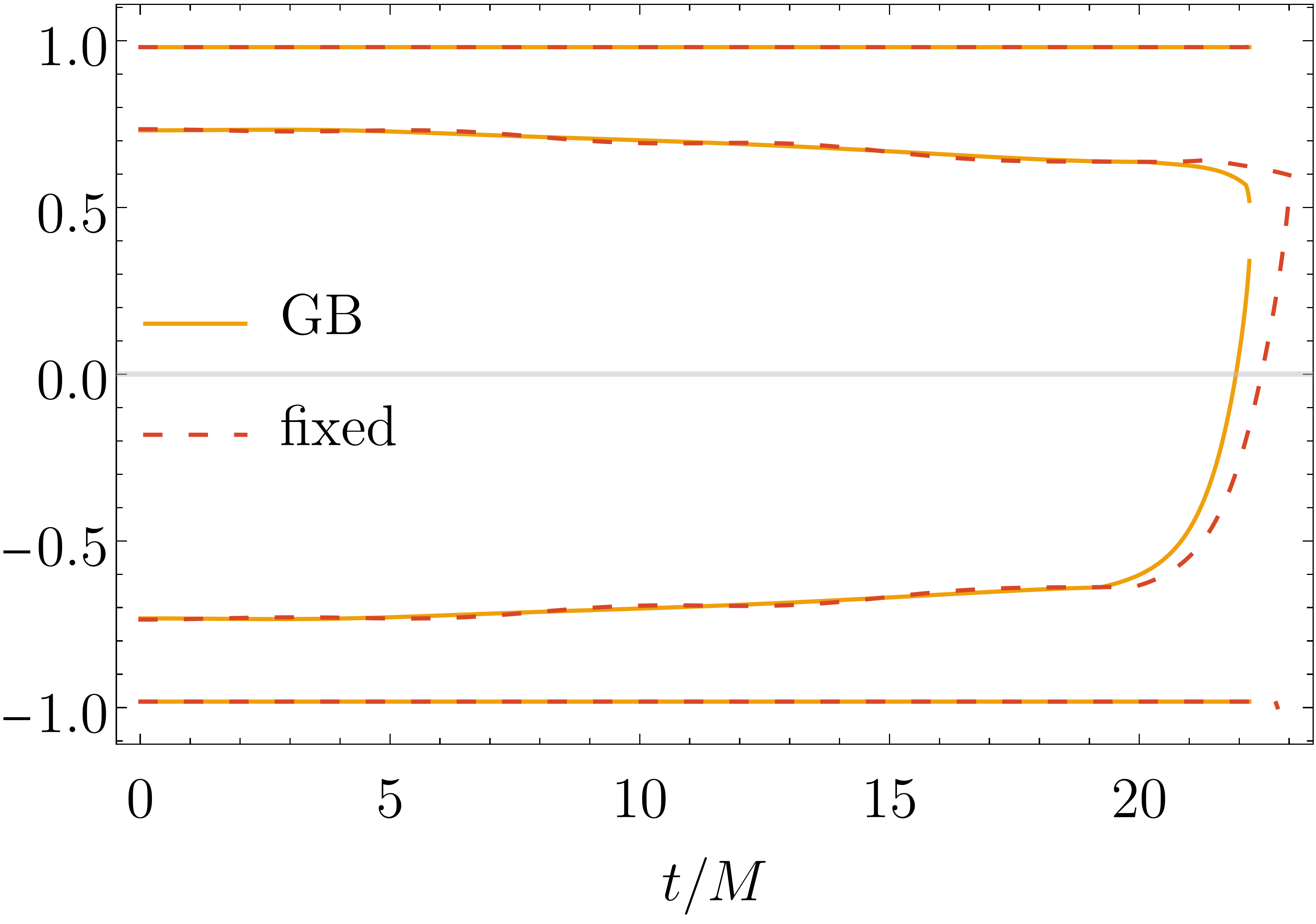
Figure 1: A comparison of the maximum and the minimum of $\bar{v}^{\text{\tiny{GB}}}_{\pm}$ and $v^{\text{\tiny{GB}}}_{\pm}$, respectively represented by a yellow solid line and a red dashed line. From top to bottom, we show $\max(v_{+})$, $\min(v_{+})$, $\max(v_{-})$, $\min(v_{-})$.

First of all, we show that gravitational collapse in the full and fixed theories produces approximately the same dynamics. We evolve the same pulse in the two theories with the choice of parameters summarized in Table 2, with labels EV1 and EV2. In the comparison, we pay attention to the characteristic speeds of the theories. In Figure 1 we plot, as a function of time, the maximum and minimum of $\bar{v}^{\text{\tiny{GB}}}_{\pm}$ and ${v}^{\text{\tiny{GB}}}_{\pm}$. We stress that the functional form of the two quantities is the same, and a bar (no bar) denotes quantities evaluated in the full (fixed) theory. During the first stage of the gravitational collapse, around $t\leq 15M$, the characteristic speeds are almost indistinguishable and constant during the evolution, showing that the character of the full theory is strongly hyperbolic and well reproduced by the fixed one. Nevertheless, at $t\sim 22M,$ one of the characteristic speeds crosses zero becoming imaginary shortly after, and therefore the system changes character from hyperbolic to elliptic. It is worth noting that even if the equations in the fixed system are different, their variables reproduce quite well the breaking of hyperbolicity of the full theory. We recall that the true characteristic speeds of the fixed problem are $v^{\text{\tiny{F}}}_{\pm}$, and that they never change sign. This means that for every case, for $t\gtrsim 22M$ the full theory cannot be evolved, but we can always follow the evolution of the fixed system.

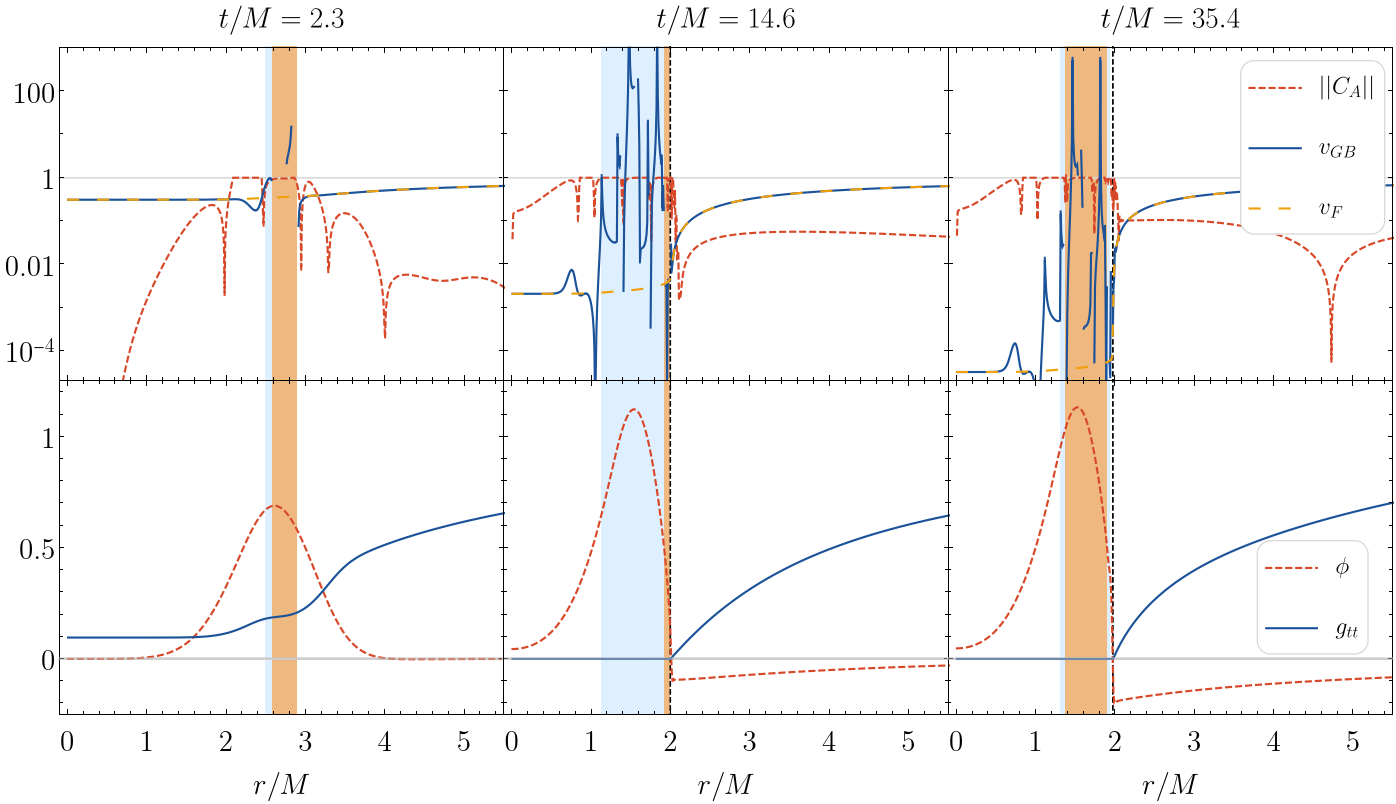
Figure 2: Top panel: snapshots of characteristic speeds $v_{+}^{\text{\tiny{GB}}}$ and $v_{+}^{\text{\tiny{F}}}$ (blue solid and yellow long-dashed lines respectively) compared to the relative difference between $C_{A}^{\text{\tiny{GB}}}$ and $C_{A}^{\text{\tiny{F}}}$ (red short-dashed line). Bottom panel: scalar field $\phi$ (red dashed line) and lapse $\mathrm{e}^{A}$ (blue solid line). The first snapshot is when the elliptic region forms in the full theory. The second snapshot is when the apparent horizon forms in the fixed theory. The third snapshot is at a late time when the scalarized profile appeared in the fixed theory. The light blue area corresponds to the region where $v_{+}^{\text{\tiny{GB}}}<0$ or $v_{+}^{\text{\tiny{GB}}}>1$, the orange area corresponds to the elliptic region (in the full system) where $\mathpzc{D}<0$, while the black dashed vertical line in the second and third panels is the location of the apparent horizon.

With this in mind, we evolve a pulse in the fixed theory, for a choice of parameters that would break hyperbolicity in the full theory. In Figure 2, we give an estimate of how the full theory would behave, by computing the quantities of this theory with the variables of the fixed one. Here, we plot time snapshots of the evolution EV3, summarized in Table (2). In the top panels, we show the characteristic speeds, $v_{\pm}^{\text{\tiny{GB}}}$ and $v_{\pm}^{\text{\tiny{F}}}$, and the norm $||C_{A}||$. In the bottom panels we show the scalar profile $\phi$ and $g_{tt}$. The first panel shows results at $t=2.3M$. One can see that the full system would develop an elliptic character, confined only in a limited region of space where the characteristic speeds would become imaginary and $\mathpzc{D}<0$. This region is denoted by an orange vertical strip. Moreover, we plot a blue region defined by the conditions $v_{\pm}^{\text{\tiny{GB}}}<0$ or $v_{\pm}^{\text{\tiny{GB}}}>1$. This region roughly corresponds to that where the deviation between $C_{A}^{\text{\tiny{F}}}$ and $C_{A}^{\text{\tiny{GB}}}$ becomes noticeable. This pattern remains in the second and third panels, the former being a snapshot at BH formation at $t\simeq 14.6M$, while the latter is a snapshot of the later evolution at $t=35.4M$, where we expect scalarization of the BH.

It is worth noticing that the region where $||v_{\pm}||$ is of order $1$ also corresponds to that where the equations of the two theories differ significantly. Outside this region, the equations and speeds of the two theories are very close. Thus, we conjecture that the physical evolution of the scalar field outside the region where $||v_{\pm}||\sim 1$ is trustworthy. We checked that this behavior persists at late times, when the scalar field grows considerably, as a result of spontaneous scalarization.

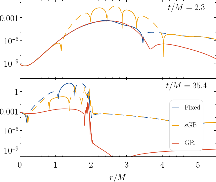
Figure 3: Null convergence condition. Each line corresponds to a radial snapshot of the NCC evaluated in the fixed system (blue line), in the full system (yellow line) or with a minimally coupled scalar field (red line). Solid lines correspond to positive NCC, while dashed lines correspond to negative NCC. The top panel shows a snapshot at $t=2.3M$ (roughly corresponding to the appearance of an elliptic region in the full system), while the bottom panel shows the late behavior of the system at $t=35.4M$.

Another way to understand how the fixing works consists of evaluating the NCC. In Fig. 3 we compare the condition for the fixed system, for the full one evaluated with quantities in the fixed system, and for an evolution with equivalent initial data, but with a minimally coupled scalar field (labelled as EV4 in Table 2). We can see that at the formation of the elliptic region (upper panel), the NCC of the fixed system resembles that of GR at small radii, while it almost overlaps with the condition evaluated for the full system at large radii. This latter trend persists throughout the whole evolution, as one can notice in the lower panel of the figure, evaluated at $t=35.4M$. The absolute value of the NCC is here expressed in logarithmic scale, we denote the regions where it becomes negative by a dashed line style. These results agree with expectations based on the analysis carried in Ripley and Pretorius (2019b).

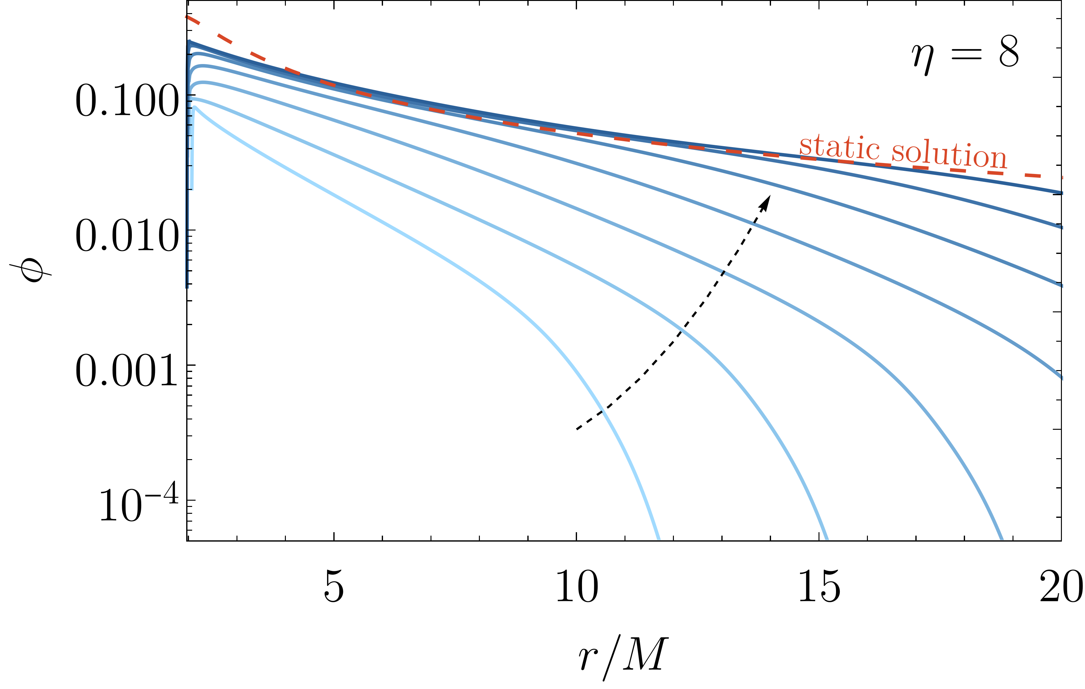
Figure 4: Scalar field profile for the scalar field. The blue solid lines are time snapshots of the radial profile outside the apparent horizon (after it has formed) as extracted from our simulations, for $\eta=8$ and $\zeta=-6\eta$. The direction of the evolution is marked by the dotted black arrow, and by the lines getting darker. The red dashed line approached by late-time evolutions of the scalar field is the radial profile in the static case.

The previous analysis heuristically shows that the numerical evolution of the fixed theory is reliable, especially outside the apparent horizon (when the latter forms). Thus, we evolved a few cases with different combinations of $\eta$ and $\zeta$ to see whether spontaneous scalarization of the final BH that forms from the collapse is achieved. We consider one representative case, summarized in Table 2 as EV5. The results for the gravitational collapse of this case are shown in Fig. 4. The blue lines indicate time snapshots of the radial profile of the scalar field $\phi$ after the formation of an apparent horizon. After the collapse, the scalar field surrounding the BH settles down to a static solution. We compare this equilibrium configuration with the one obtained by solving the static spherical problem in the full theory (c.f. Silva et al. (2019)). This static solution can be obtained simply by requiring all the functions to be time-independent, or equivalently by replacing $\partial_{t}\phi=\partial_{t}P=\partial_{t}Q=0,$ in Eqs. (3)–(4). By doing so, the equations are reduced to a set of ordinary differential equations, which can be easily integrated by imposing proper boundary conditions at the horizon of the BH and asymptotic flatness at the outer boundary. We clearly see that the evolution drives the scalar field to match the static profile. We stress that we obtained similar results with different values of the coupling and different choices of initial data.

A few caveats to discuss are the following. The dynamical evolution of the scalar field does not seem to asymptote well to the static solution in a region very close to the apparent horizon. We conjecture that this behaviour is due to a small portion of the elliptic region of the full theory leaking out of the horizon. Therefore, even if we can “heal” the character of the field equations in the fixed theory, we still expect some discrepancy in this region of large gradients and high-frequency energy flows. On the other hand, the scalar field does not fully match the static case at large radii either, but this is simply because we could not run the evolution any longer. At the level of implementation, possible improvements include using horizon penetrating coordinates rather than polar coordinates and/or excising the region inside the apparent horizon.

In order to understand how the fixing behaves, we studied the effect of different values of $\xi$ and $\tau$. We are interested in the limit $\tau\rightarrow 0$ and $\xi\rightarrow 0$. However, note that for values of $\xi$ lower than the coupling constant $\eta$, the evolution breaks down at early stages and cannot be followed, as expected from Cayuso et al. (2017). This is an issue that can be addressed by coupling both parameters in a suitable manner. Otherwise, since the decay rate is $\approx\tau/\xi$, adopting too small a $\xi$ value would yield a stiff system, which needs to be handled with care at the numerical level. In our simulations we could set $\tau$ identically to zero as the results do not change with respect to cases where $\tau/\eta\ll 1$.

Notice that a static, radially dependent, solution would induce a discrepancy between $\bf{u}$ and $\bf{S}$ given by $\approx\xi\nabla^{2}\bf{u}$. One can recover the static behavior as $\xi\rightarrow 0$ for the particular fixing employed. Here, we employ a single value for $\xi$. For completeness, we also checked cases where we adopt five different constants—one for each auxiliary field—and found that we can lower a subset of these constants, while still getting a proper evolution. Namely, by lowering by a factor 10 the constants controlling the equations for $\Sigma$, $\Gamma_{22}$ and $\Gamma_{33}$, we observed that the results obtained do not qualitatively change.

On the other hand, in Fig. 5 we show the effects of increasing $\xi$. The three panels are analogous to Fig. 4, but with $\eta=6$ and $\zeta=-6\eta$, and each of them assumes an increasing value of $\xi$. The runs correspond to EV3, EV6 and EV7 in Tab. 2, respectively. It is clear that the scalar evolution matches well the static prediction only for the lowest value of $\xi$. This is not surprising, as large values of $\xi$ imply that the fixed system’s faithfulness to the original one degrades.

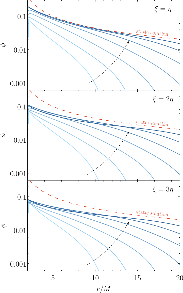
Figure 5: Same as Fig. 4, but with for $\eta=6$, $\zeta=-6\eta$ and different values of $\xi$.

V Conclusions

In the current work we studied the dynamical collapse and related hair BH formation in sGB gravity. Such a theory has been the subject of scrutiny in recent years, which has revealed interesting behaviors for BH physics Silva et al. (2018); Doneva and Yazadjiev (2018); Antoniou et al. (2018); Silva et al. (2019); Cunha et al. (2019); Dima et al. (2020); Herdeiro et al. (2021); Berti et al. (2021). However, as it has been discussed elsewhere Ripley and Pretorius (2019a, b, 2020); Witek et al. (2020); Julié and Berti (2020), it also presents important mathematical challenges in regimes of high couplings and/or short wavelengths. Such challenges stem from the equations of motion breaking their hyperbolic character. This makes it impossible to explore important questions such as the formation and non-linear stability of compact objects, unless further steps are taken to address the the theory’s shortcomings. Further, even in the weak coupling regime, physical effects abound that induce short wavelength behavior from long wavelength, e.g., focusing and collapse. For instance, a gravitational (or scalar) wave passing by a BH could be focused and excite significantly short wavelengths, potentially breaking (local) hyperbolicity. Unless a BH generically shields such regions away from physical observers, one could argue that extensions of GR that present these shortcomings would have limited physical relevance. It behooves theorists to try and devise ways to explore such question.

Here, we adopted a strategy dubbed as fixing-the-equations, which introduces further auxiliary fields, constrained within some given scale, to force a suitably modified system to agree with the original equations of motion, while at the same time controlling the behavior at shorter wavelengths Cayuso et al. (2017). This approach, to a certain extent, recovers some of the higher energy degrees of freedom, which in an effective field theory sense are integrated out and whose influence results in corrections to the Einstein-Hilbert action. Controlling the high frequency modes of the solution, this approach eliminates (or significantly reduces) the mathematical pathologies of the original system, thus allowing one to push evolutions further. Note that the fixing approach breaks Lorentz symmetry, in particular through the $\tau$-term in Eq. (10) which sets a scale—in time and wavelength—below which such breaking is especially evident. The presence of this term is in agreement with the fact that the UV completion of the theory has to be non-standard Herrero-Valea (2022).

In our particular application, the fixing allowed us to resolve the collapse to a scalarized BH. Remarkably, this dynamically formed BH agrees with static solutions of the original unfixed theory. We stress that this was not necessarily expected, as our method does introduce modifications in the theory. As such, the agreement of the solutions found is highly non-trivial and indicates that the fixed system successfully bridges between stages where/when the original system is well behaved. We also stress that we find regimes where hyperbolicity breaks outside the apparent horizon for sGB as already noted in previous works Ripley and Pretorius (2019a, a, 2020); East and Ripley (2021b, a). Two comments are in order here: (i) that sGB shows fails to be hyperbolic outside the horizon implies one can not assume that a horizon will hide such failure from outside observers. (ii) this failure should not happen in a proper UV completion of the theory, and the fixed version allows to by pass such issue. Last, we note that the fixed system yields a solution that approaches the one expected in the static regime. This is analogous to the behavior observed in an effective-field-theory-derived gravitational theory where BH accretion was studied and the late time solution agreed with the static one Cayuso and Lehner (2020). If this observed robustness could be extrapolated to more general solutions and other extensions to GR, it would lend strong support to the physical relevance of such solutions and conclusions drawn from perturbative studies. Furthermore, this agreement supports the idea that the approach employed can be regarded as furnishing a weak completion of the original theory.

Appendix A Code validation

Here we present the details about the convergence tests performed to validate our simulations. We evolve the fixed theory considering two representatives cases: (i) EV8 (see Table 2), where a small pulse just grows as it approaches to the origin and then disperses to infinity, and (ii) EV3, where the pulse collapses to form an apparent horizon, with a non-trivial scalar profile outside. Our simulations are evolved by using three different resolutions $\{\Delta r_{\text{\rm{low}}},\Delta r_{\text{\rm{med}}},\Delta r_{\text{\rm{high}}}\}=\{0.0625,0.03125,0.015625\}$. We compute the convergence factor $c_{p}$ and the order of convergence as follows

$$c_{p}=\frac{\left|(\Delta r_{\text{\rm{low}}})^{p}-(\Delta r_{\text{\rm{med}}})^{p}\right|}{|(\Delta r_{\text{\rm{med}}})^{p}-(\Delta r_{\text{\rm{high}}})^{p}|}\,.$$ (48)

We use the Misner-Sharp mass (38) to compute $c_{p}$ and $p$, as shown in Fig. 6. In the top panel, we show the convergence for EV8, finding a fourth order convergence as expected. In the lower panel the convergence for EV3 is displayed. In this case, until the collapse we find fourth-order convergence, but after the formation of the apparent horizon the convergence is somewhat degraded. This is expected due to the large gradients in the collapse front.

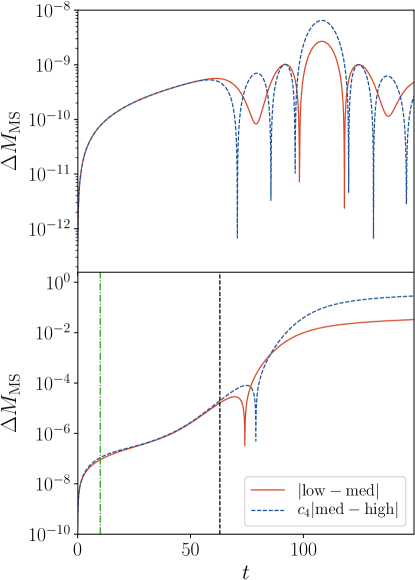
Figure 6: Convergence for the Misner-Sharp mass for the cases EV8 and EV3 respectively. We display in both panels the absolute difference between the low and medium resolutions (solid red line) and the medium and high resolutions (dashed blue line). The latter is rescaled by a factor $c_{4}=16$ in both cases, showing fourth order convergence. The green dot-dashed line denotes the time when the elliptic region in the full theory appears, and the dashed black line indicates when the BH is formed.

Appendix B Source of the fixed equations

In this Appendix we show the explicit form of the source terms $\mathbf{S}$ appearing in equation (10)

$$\begin{split}S_{\Sigma}=f^{\prime}(\phi_{0})\Bigg{[}&\frac{16\mathrm{e}^{-4B}\partial_{r}A\partial_{r}B+2\left(\mathrm{e}^{2B}-\mathrm{e}^{-2B}\right)\left(P^{2}-Q^{2}\right)}{r^{2}}-\frac{8\left(\mathrm{e}^{2B}-\mathrm{e}^{-2B}\right)\left(\partial_{r}A-\partial_{r}B\right)}{r^{3}}\left.-\mathrm{e}^{-4B}\Delta^{2}+\frac{8y\Gamma_{33}}{r^{4}}\right]\,,\end{split}$$ (49a)

$$\begin{split}S_{11}=\mathrm{e}^{2A-2B}f^{\prime}(\phi_{0})\Bigg{[}\frac{4\left(\left(3\mathrm{e}^{-2B}-1\right)Q\partial_{r}B+y\partial_{r}Q\right)}{r^{2}}-\left.\frac{yP\Delta}{r}\right]+\frac{4y\,\mathrm{e}^{2A-2B}f^{\prime\prime}(\phi_{0})Q^{2}}{r^{2}}\,,\end{split}$$ (49b)

$$\begin{split}S_{12}=-\mathrm{e}^{A-B}f^{\prime}(\phi_{0})\Bigg{[}&\frac{4y\left(P\partial_{r}B-\partial_{r}P\right)}{r^{2}}+\frac{\left(1-3\mathrm{e}^{-2B}\right)Q\Delta}{r}\Bigg{]}+\frac{4yf^{\prime\prime}(\phi_{0})PQ\mathrm{e}^{A-B}}{r^{2}}\,,\end{split}$$ (49c)

$$\begin{split}S_{22}=f^{\prime}(\phi_{0})\Bigg{[}&\frac{8\mathrm{e}^{-2B}Q\partial_{r}A-4y\left(Q\partial_{r}B-\partial_{r}Q+\mathrm{e}^{2B}\Sigma\right)}{r^{2}}\left.-\frac{yP\Delta}{r}+\frac{8yQ}{r^{3}}\right]+\frac{4yf^{\prime\prime}(\phi_{0})P^{2}}{r^{2}}\,,\end{split}$$ (49d)

$$\begin{split}S_{33}=\mathrm{e}^{-4B}f^{\prime}(\phi_{0})\Bigg{[}&r\bigg{(}\!-4\partial_{r}B\left(Q\partial_{r}A-\partial_{r}Q+\mathrm{e}^{2B}\Sigma\right)+4\partial_{r}A\partial_{r}Q-4Q\left(\partial_{r}B\right)^{2}+P^{2}Q-Q^{3}\bigg{)}\\ &-r^{2}\left(P\partial_{r}A-P\partial_{r}B+2\partial_{r}P\right)\Delta\left.-4Q\left(\partial_{r}A-3\partial_{r}B\right)+\frac{1}{2}Qr^{3}\Delta^{2}+\frac{4\mathrm{e}^{2B}\Gamma_{33}Q}{r}\right]\\ +2e^{-4B}f^{\prime\prime}(\phi_{0})\bigg{[}&2r\left(Q^{2}\partial_{r}A+P^{2}\partial_{r}B\right)-PQr^{2}\Delta\bigg{]}\,,\end{split}$$ (49e)

with $y=\left(1-\mathrm{e}^{-2B}\right)$ and $\Delta=\left(PQ+2\mathrm{e}^{B-A}\Gamma_{12}\right)$.

References

- Abbott et al. (2016) B. P. Abbott et al. (LIGO Scientific, Virgo), “Tests of general relativity with GW150914,” Phys. Rev. Lett. 116, 221101 (2016), [Erratum: Phys.Rev.Lett. 121, 129902 (2018)], arXiv:1602.03841 [gr-qc] .
- Abbott et al. (2019) B. P. Abbott et al. (LIGO Scientific, Virgo), “Tests of General Relativity with the Binary Black Hole Signals from the LIGO-Virgo Catalog GWTC-1,” Phys. Rev. D 100, 104036 (2019), arXiv:1903.04467 [gr-qc] .
- Abbott et al. (2021a) R. Abbott et al. (LIGO Scientific, Virgo), “Tests of general relativity with binary black holes from the second LIGO-Virgo gravitational-wave transient catalog,” Phys. Rev. D 103, 122002 (2021a), arXiv:2010.14529 [gr-qc] .
- Abbott et al. (2021b) R. Abbott et al. (LIGO Scientific, VIRGO, KAGRA), “Tests of General Relativity with GWTC-3,” (2021b), arXiv:2112.06861 [gr-qc] .
- Barausse et al. (2013) Enrico Barausse, Carlos Palenzuela, Marcelo Ponce, and Luis Lehner, “Neutron-star mergers in scalar-tensor theories of gravity,” Phys. Rev. D 87, 081506 (2013), arXiv:1212.5053 [gr-qc] .
- Palenzuela et al. (2014) Carlos Palenzuela, Enrico Barausse, Marcelo Ponce, and Luis Lehner, “Dynamical scalarization of neutron stars in scalar-tensor gravity theories,” Phys. Rev. D 89, 044024 (2014), arXiv:1310.4481 [gr-qc] .
- Shibata et al. (2014) Masaru Shibata, Keisuke Taniguchi, Hirotada Okawa, and Alessandra Buonanno, “Coalescence of binary neutron stars in a scalar-tensor theory of gravity,” Phys. Rev. D 89, 084005 (2014), arXiv:1310.0627 [gr-qc] .
- Hirschmann et al. (2018) Eric W. Hirschmann, Luis Lehner, Steven L. Liebling, and Carlos Palenzuela, “Black Hole Dynamics in Einstein-Maxwell-Dilaton Theory,” Phys. Rev. D 97, 064032 (2018), arXiv:1706.09875 [gr-qc] .
- Bezares et al. (2022) Miguel Bezares, Ricard Aguilera-Miret, Lotte ter Haar, Marco Crisostomi, Carlos Palenzuela, and Enrico Barausse, “No Evidence of Kinetic Screening in Simulations of Merging Binary Neutron Stars beyond General Relativity,” Phys. Rev. Lett. 128, 091103 (2022), arXiv:2107.05648 [gr-qc] .
- Figueras and França (2021) Pau Figueras and Tiago França, “Black Hole Binaries in Cubic Horndeski Theories,” (2021), arXiv:2112.15529 [gr-qc] .
- Papallo and Reall (2017) Giuseppe Papallo and Harvey S. Reall, “On the local well-posedness of Lovelock and Horndeski theories,” Phys. Rev. D 96, 044019 (2017), arXiv:1705.04370 [gr-qc] .
- Ripley and Pretorius (2019a) Justin L. Ripley and Frans Pretorius, “Hyperbolicity in Spherical Gravitational Collapse in a Horndeski Theory,” Phys. Rev. D 99, 084014 (2019a), arXiv:1902.01468 [gr-qc] .
- Ripley and Pretorius (2019b) Justin L. Ripley and Frans Pretorius, “Gravitational collapse in Einstein dilaton-Gauss–Bonnet gravity,” Class. Quant. Grav. 36, 134001 (2019b), arXiv:1903.07543 [gr-qc] .
- Ripley and Pretorius (2020) Justin L. Ripley and Frans Pretorius, “Dynamics of a symmetric EdGB gravity in spherical symmetry,” Class. Quant. Grav. 37, 155003 (2020), arXiv:2005.05417 [gr-qc] .
- Bernard et al. (2019) Laura Bernard, Luis Lehner, and Raimon Luna, “Challenges to global solutions in Horndeski’s theory,” Phys. Rev. D 100, 024011 (2019), arXiv:1904.12866 [gr-qc] .
- Bezares et al. (2021a) Miguel Bezares, Marco Crisostomi, Carlos Palenzuela, and Enrico Barausse, “K-dynamics: well-posed 1+1 evolutions in K-essence,” JCAP 03, 072 (2021a), arXiv:2008.07546 [gr-qc] .
- Horndeski (1974) Gregory Walter Horndeski, “Second-order scalar-tensor field equations in a four-dimensional space,” Int. J. Theor. Phys. 10, 363–384 (1974).
- Ostrogradsky (1850) M. Ostrogradsky, “Mémoires sur les équations différentielles, relatives au problème des isopérimètres,” Mem. Acad. St. Petersbourg 6, 385–517 (1850).
- Hui and Nicolis (2013) Lam Hui and Alberto Nicolis, “No-Hair Theorem for the Galileon,” Phys. Rev. Lett. 110, 241104 (2013), arXiv:1202.1296 [hep-th] .
- Sotiriou and Zhou (2014a) Thomas P. Sotiriou and Shuang-Yong Zhou, “Black hole hair in generalized scalar-tensor gravity: An explicit example,” Phys. Rev. D 90, 124063 (2014a), arXiv:1408.1698 [gr-qc] .
- Sotiriou and Zhou (2014b) Thomas P. Sotiriou and Shuang-Yong Zhou, “Black hole hair in generalized scalar-tensor gravity,” Phys. Rev. Lett. 112, 251102 (2014b), arXiv:1312.3622 [gr-qc] .
- Silva et al. (2018) Hector O. Silva, Jeremy Sakstein, Leonardo Gualtieri, Thomas P. Sotiriou, and Emanuele Berti, “Spontaneous scalarization of black holes and compact stars from a Gauss-Bonnet coupling,” Phys. Rev. Lett. 120, 131104 (2018), arXiv:1711.02080 [gr-qc] .
- Doneva and Yazadjiev (2018) Daniela D. Doneva and Stoytcho S. Yazadjiev, “New Gauss-Bonnet Black Holes with Curvature-Induced Scalarization in Extended Scalar-Tensor Theories,” Phys. Rev. Lett. 120, 131103 (2018), arXiv:1711.01187 [gr-qc] .
- Antoniou et al. (2018) G. Antoniou, A. Bakopoulos, and P. Kanti, “Evasion of No-Hair Theorems and Novel Black-Hole Solutions in Gauss-Bonnet Theories,” Phys. Rev. Lett. 120, 131102 (2018), arXiv:1711.03390 [hep-th] .
- Silva et al. (2019) Hector O. Silva, Caio F. B. Macedo, Thomas P. Sotiriou, Leonardo Gualtieri, Jeremy Sakstein, and Emanuele Berti, “Stability of scalarized black hole solutions in scalar-Gauss-Bonnet gravity,” Phys. Rev. D 99, 064011 (2019), arXiv:1812.05590 [gr-qc] .
- Cunha et al. (2019) Pedro V. P. Cunha, Carlos A. R. Herdeiro, and Eugen Radu, “Spontaneously Scalarized Kerr Black Holes in Extended Scalar-Tensor–Gauss-Bonnet Gravity,” Phys. Rev. Lett. 123, 011101 (2019), arXiv:1904.09997 [gr-qc] .
- Dima et al. (2020) Alexandru Dima, Enrico Barausse, Nicola Franchini, and Thomas P. Sotiriou, “Spin-induced black hole spontaneous scalarization,” Phys. Rev. Lett. 125, 231101 (2020), arXiv:2006.03095 [gr-qc] .
- Herdeiro et al. (2021) Carlos A. R. Herdeiro, Eugen Radu, Hector O. Silva, Thomas P. Sotiriou, and Nicolás Yunes, “Spin-induced scalarized black holes,” Phys. Rev. Lett. 126, 011103 (2021), arXiv:2009.03904 [gr-qc] .
- Berti et al. (2021) Emanuele Berti, Lucas G. Collodel, Burkhard Kleihaus, and Jutta Kunz, “Spin-induced black-hole scalarization in Einstein-scalar-Gauss-Bonnet theory,” Phys. Rev. Lett. 126, 011104 (2021), arXiv:2009.03905 [gr-qc] .
- Antoniou et al. (2021) Georgios Antoniou, Antoine Lehébel, Giulia Ventagli, and Thomas P. Sotiriou, “Black hole scalarization with Gauss-Bonnet and Ricci scalar couplings,” Phys. Rev. D 104, 044002 (2021), arXiv:2105.04479 [gr-qc] .
- Antoniou et al. (2022) Georgios Antoniou, Caio F. B. Macedo, Ryan McManus, and Thomas P. Sotiriou, “Stable spontaneously-scalarized black holes in generalized scalar-tensor theories,” (2022), arXiv:2204.01684 [gr-qc] .
- Damour and Esposito-Farese (1993) Thibault Damour and Gilles Esposito-Farese, “Nonperturbative strong field effects in tensor - scalar theories of gravitation,” Phys. Rev. Lett. 70, 2220–2223 (1993).
- Andreou et al. (2019) Nikolas Andreou, Nicola Franchini, Giulia Ventagli, and Thomas P. Sotiriou, “Spontaneous scalarization in generalised scalar-tensor theory,” Phys. Rev. D 99, 124022 (2019), [Erratum: Phys.Rev.D 101, 109903 (2020)], arXiv:1904.06365 [gr-qc] .
- Ventagli et al. (2020) Giulia Ventagli, Antoine Lehébel, and Thomas P. Sotiriou, “Onset of spontaneous scalarization in generalized scalar-tensor theories,” Phys. Rev. D 102, 024050 (2020), arXiv:2006.01153 [gr-qc] .
- Eardley et al. (1973) Douglas M. Eardley, David L. Lee, and Alan P. Lightman, “Gravitational-wave observations as a tool for testing relativistic gravity,” Phys. Rev. D 8, 3308–3321 (1973).
- Will (2006) Clifford M. Will, “The Confrontation between general relativity and experiment,” Living Rev. Rel. 9, 3 (2006), arXiv:gr-qc/0510072 .
- Barausse et al. (2016) Enrico Barausse, Nicolás Yunes, and Katie Chamberlain, “Theory-Agnostic Constraints on Black-Hole Dipole Radiation with Multiband Gravitational-Wave Astrophysics,” Phys. Rev. Lett. 116, 241104 (2016), arXiv:1603.04075 [gr-qc] .
- Silva et al. (2021) Hector O. Silva, Helvi Witek, Matthew Elley, and Nicolás Yunes, “Dynamical Descalarization in Binary Black Hole Mergers,” Phys. Rev. Lett. 127, 031101 (2021), arXiv:2012.10436 [gr-qc] .
- East and Ripley (2021a) William E. East and Justin L. Ripley, “Dynamics of Spontaneous Black Hole Scalarization and Mergers in Einstein-Scalar-Gauss-Bonnet Gravity,” Phys. Rev. Lett. 127, 101102 (2021a), arXiv:2105.08571 [gr-qc] .
- Doneva et al. (2022) Daniela D. Doneva, Alex Vañó Viñuales, and Stoytcho S. Yazadjiev, “Dynamical descalarization with a jump during black hole merger,” (2022), arXiv:2204.05333 [gr-qc] .
- Elley et al. (2022) Matthew Elley, Hector O. Silva, Helvi Witek, and Nicolás Yunes, “Spin-induced dynamical scalarization, de-scalarization and stealthness in scalar-Gauss-Bonnet gravity during black hole coalescence,” (2022), arXiv:2205.06240 [gr-qc] .
- Benkel et al. (2016) Robert Benkel, Thomas P. Sotiriou, and Helvi Witek, “Dynamical scalar hair formation around a Schwarzschild black hole,” Phys. Rev. D 94, 121503 (2016), arXiv:1612.08184 [gr-qc] .
- Benkel et al. (2017) Robert Benkel, Thomas P. Sotiriou, and Helvi Witek, “Black hole hair formation in shift-symmetric generalised scalar-tensor gravity,” Class. Quant. Grav. 34, 064001 (2017), arXiv:1610.09168 [gr-qc] .
- East and Ripley (2021b) William E. East and Justin L. Ripley, “Evolution of Einstein-scalar-Gauss-Bonnet gravity using a modified harmonic formulation,” Phys. Rev. D 103, 044040 (2021b), arXiv:2011.03547 [gr-qc] .
- Corelli et al. (2022a) Fabrizio Corelli, Marina De Amicis, Taishi Ikeda, and Paolo Pani, “What is the fate of Hawking evaporation in gravity theories with higher curvature terms?” (2022a), arXiv:2205.13006 [gr-qc] .
- Corelli et al. (2022b) Fabrizio Corelli, Marina De Amicis, Taishi Ikeda, and Paolo Pani, “Nonperturbative gedanken experiments in Einstein-dilaton-Gauss-Bonnet gravity: nonlinear transitions and tests of the cosmic censorship beyond General Relativity,” (2022b), arXiv:2205.13007 [gr-qc] .
- Hadamard (1902) J. Hadamard, “Sur les problemes aux derivees partielles et leur signification physique,” Princeton university bulletin , 49–52 (1902).
- Evans (2010) Lawrence C. Evans, Partial differential equations (American Mathematical Society, Providence, R.I., 2010).
- Hilditch (2013) David Hilditch, “An Introduction to Well-posedness and Free-evolution,” Int. J. Mod. Phys. A 28, 1340015 (2013), arXiv:1309.2012 [gr-qc] .
- Sarbach and Tiglio (2012) Olivier Sarbach and Manuel Tiglio, “Continuum and Discrete Initial-Boundary-Value Problems and Einstein’s Field Equations,” Living Rev. Rel. 15, 9 (2012), arXiv:1203.6443 [gr-qc] .
- Kovács and Reall (2020a) Áron D. Kovács and Harvey S. Reall, “Well-Posed Formulation of Scalar-Tensor Effective Field Theory,” Phys. Rev. Lett. 124, 221101 (2020a), arXiv:2003.04327 [gr-qc] .
- Kovács and Reall (2020b) Áron D. Kovács and Harvey S. Reall, “Well-posed formulation of Lovelock and Horndeski theories,” Phys. Rev. D 101, 124003 (2020b), arXiv:2003.08398 [gr-qc] .
- Cayuso et al. (2017) Juan Cayuso, Néstor Ortiz, and Luis Lehner, “Fixing extensions to general relativity in the nonlinear regime,” Phys. Rev. D 96, 084043 (2017), arXiv:1706.07421 [gr-qc] .
- Allwright and Lehner (2019) Gwyneth Allwright and Luis Lehner, “Towards the nonlinear regime in extensions to GR: assessing possible options,” Class. Quant. Grav. 36, 084001 (2019), arXiv:1808.07897 [gr-qc] .
- Cayuso and Lehner (2020) Ramiro Cayuso and Luis Lehner, “Nonlinear, noniterative treatment of EFT-motivated gravity,” Phys. Rev. D 102, 084008 (2020), arXiv:2005.13720 [gr-qc] .
- Bezares et al. (2021b) Miguel Bezares, Lotte ter Haar, Marco Crisostomi, Enrico Barausse, and Carlos Palenzuela, “Kinetic screening in nonlinear stellar oscillations and gravitational collapse,” Phys. Rev. D 104, 044022 (2021b), arXiv:2105.13992 [gr-qc] .
- Lara et al. (2022) Guillermo Lara, Miguel Bezares, and Enrico Barausse, “UV completions, fixing the equations, and nonlinearities in k-essence,” Phys. Rev. D 105, 064058 (2022), arXiv:2112.09186 [gr-qc] .
- Gerhardinger et al. (2022) Mary Gerhardinger, John T. Giblin, Andrew J. Tolley, and Mark Trodden, “A Well-Posed UV Completion for Simulating Scalar Galileons,” (2022), arXiv:2205.05697 [hep-th] .
- Julié and Berti (2019) Félix-Louis Julié and Emanuele Berti, “Post-Newtonian dynamics and black hole thermodynamics in Einstein-scalar-Gauss-Bonnet gravity,” Phys. Rev. D 100, 104061 (2019), arXiv:1909.05258 [gr-qc] .
- Israel and Stewart (1976) W. Israel and J. M. Stewart, “Thermodynamics of nonstationary and transient effects in a relativistic gas,” Physics Letters A 58, 213–215 (1976).
- Israel (1976) W. Israel, “Nonstationary irreversible thermodynamics: A Causal relativistic theory,” Annals Phys. 100, 310–331 (1976).
- Muller (1967) Ingo Muller, “Zum Paradoxon der Warmeleitungstheorie,” Z. Phys. 198, 329–344 (1967).
- Misner and Sharp (1964) Charles W. Misner and David H. Sharp, “Relativistic equations for adiabatic, spherically symmetric gravitational collapse,” Phys. Rev. 136, B571–B576 (1964).
- Bardeen et al. (1973) James M. Bardeen, B. Carter, and S. W. Hawking, “The Four laws of black hole mechanics,” Commun. Math. Phys. 31, 161–170 (1973).
- Hayward (1994) S. A. Hayward, “General laws of black hole dynamics,” Phys. Rev. D 49, 6467–6474 (1994).
- Calabrese et al. (2004) Gioel Calabrese, Luis Lehner, Oscar Reula, Olivier Sarbach, and Manuel Tiglio, “Summation by parts and dissipation for domains with excised regions,” Class. Quant. Grav. 21, 5735–5758 (2004), arXiv:gr-qc/0308007 .
- Witek et al. (2020) Helvi Witek, Leonardo Gualtieri, and Paolo Pani, “Towards numerical relativity in scalar Gauss-Bonnet gravity: decomposition beyond the small-coupling limit,” Phys. Rev. D 101, 124055 (2020), arXiv:2004.00009 [gr-qc] .
- Julié and Berti (2020) Félix-Louis Julié and Emanuele Berti, “ formalism in Einstein-scalar-Gauss-Bonnet gravity,” Phys. Rev. D 101, 124045 (2020), arXiv:2004.00003 [gr-qc] .
- Herrero-Valea (2022) Mario Herrero-Valea, “The shape of scalar Gauss-Bonnet gravity,” JHEP 03, 075 (2022), arXiv:2106.08344 [gr-qc] .