Cascade Luminance and Chrominance for Image Retouching: More Like Artist

Abstract

Photo retouching aims to adjust the luminance, contrast, and saturation of the image to make it more human aesthetically desirable. However, artists’ actions in photo retouching are difficult to quantitatively analyze. By investigating their retouching behaviors, we propose a two-stage network that brightens images first and then enriches them in the chrominance plane. Six pieces of useful information from image EXIF are picked as the network’s condition input. Additionally, hue palette loss is added to make the image more vibrant. Based on the above three aspects, Luminance-Chrominance Cascading Net(LCCNet) makes the machine learning problem of mimicking artists in photo retouching more reasonable. Experiments show that our method is effective on the benchmark MIT-Adobe FiveK dataset, and achieves state-of-the-art performance for both quantitative and qualitative evaluation.

1 Introduction

Raw images, or raw snapshots that have not been aesthetically improved by artistic intent, can significantly boost visual appeal and expressiveness with the help of computer interactive color adjustments’ editing software such as Photoshop [1] and Lightroom [2]. However, the proficient use of these tools requires years of experience and the retouching procedures become tedious and time-consuming as images grow in quantity. Automating image retouching task aims to simulate the artists’ operation to automatically beautify the image, which is the main objective of this research.

Traditional automatic retouching methods use equilibrium operations to decorate pictures, e.g. gray-world [8], histogram equalization [22] and its many variants [13; 6; 35; 31; 12]. Alternatively, filters such as fast bilateral filtering [7] and local Laplacian operator [20] can be used to enhance the visual quality of images. These methods rely on prior knowledge to design fixed features, which is difficult to deal with rich scenes. Bychkovsky et al. [4] constructed a large image retouching dataset MIT-Adobe FiveK, which is widely used by image retouching tasks. It contains 5000 original images with corresponding five experts’ retouching results, and the intermediate operations for retouching are recorded.

Deep networks use a self-learning feature expression method and can better deal with rich scenes in automatic image retouching. A deep learning-based method was proposed by Yan et.al in 2016 [37], since then, the deep neural network-based approaches have been more adopted. Roughly speaking, they can be divided into two types: global-based and local-based. The former algorithms focus on overall adjustments, these methods can be divided into curve-based [41; 5], table based [9; 38; 34], and other global coefficient adjustment methods [17; 18; 44; 19; 15; 14]. Local-based methods [21; 24; 29; 43; 11; 30; 10; 32] adjust the image at the pixel level. All these methods use only images as input, but a single image can only provide limited scene information since the shooting process is a dimensionality reduction process. In reality, as seen in Figure 1, the same blue color in the clothes and sky is decorated differently, with clothes more transparent and the sky deeper. This one-to-many mapping of the same color cannot be handled well if neglecting important shooting conditions. In the process of retouching, artists pay attention to the environment in which the photo was taken. In this research, those related information, such as exposure time and aperture, are introduced as a condition vector to get the shooting environment to handle the one-to-many mapping of colors.

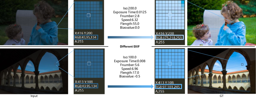
Figure 1: One-to-many color mapping and their corresponding EXIF

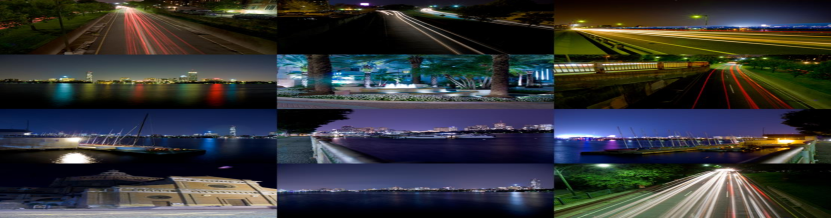
(a) Night Scene

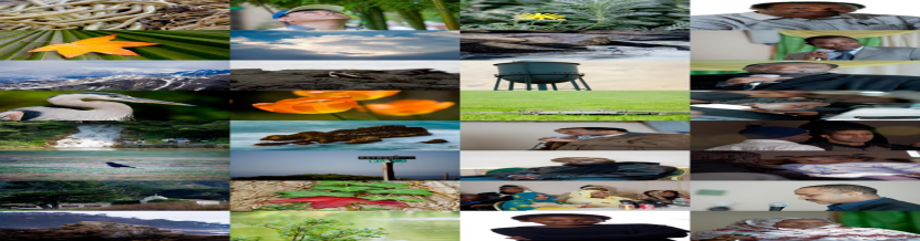
(b) Portrait

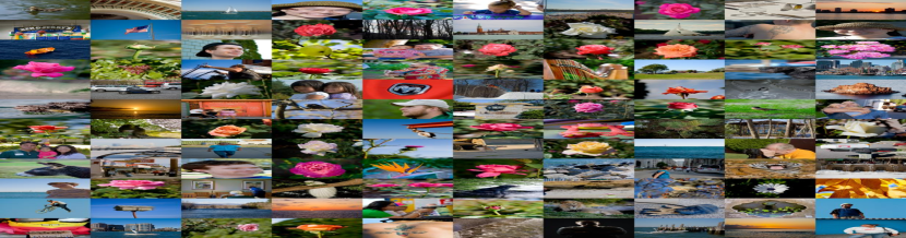
(c) Flowers

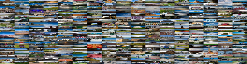
(d) Blue Sky

Figure 2: Images of some of our clustered categories

Images to be processed are usually low-light and unsaturated in the chrominance plane. Gao et.al [25] verified that the retouching task can be decomposed into two independent parametric models to adjust brightness and color separately. TSN-CA [36] uses a cascaded network to perform brightness enhancement and restoration, and the method focuses on low-light image enhancement. By researching the artist’s retouching behavior, LCCNet uses a cascaded network to adjust the image to an appropriate brightness first, then the secondary network enriches color in the chrominance plane.

$\Delta E=\sqrt{(L_{1}-L_{2})^{2}+(a_{1}-a_{2})^{2}+(b_{1}-b_{2})^{2}}$ calculates the perceptual distance of the CIE Lab color space to measure the color accuracy. A Euclidean objective function is used [42; 26] naturally based on this. However, the optimal solution to the Euclidean loss tends to the mean of set under a series of distinct $ab$ values [27]. In [27], Zhang et.al researched 1.3M training images in ImageNet [23] and found that natural images were usually with low $ab$ values and lack of high values. So using only L2 loss, the bias distribution of $ab$ values will result in mean desaturated images and cannot improve the class imbalance problem in the chrominance plane. We design the palette loss to improve the class imbalance problem by extracting color components in the hue plane and then fitting each color component independent of the number of pixels.

This paper has three main contributions:

1. We introduce six pieces of information related to the shooting condition in the EXIF as a condition vector to help handle the one-to-many mapping of colors.

2. We propose a two-stage network that brightens images first and then enriches them in the chrominance plane to simulate the artist’s operations and makes our algorithm more similar to expert retouching.

3. Hue palette loss function which balances color class in chrominance plane is proposed and makes images more saturated.

The remainder of the paper is structured as follows. The analysis of the dataset is described in Section 2. Section 3 illustrates the methodology and details of LCCNet. Section 4 reports experimental results and comparative studies between competing methods as well as ablation studies. Section 5 concludes the entire research.

2 Analysis of the dataset

2.1 Color correlation of EXIF

One of the difficulties with image retouching is that one-to-many color mapping, and identically colored input may not correspond to the same output. As shown in Figure 1, the output blue of the sky is darker with the same blue input, because the bluer sky is preferred. Obtaining conditions in which the photograph is taken (e.g.indoors and outdoors, portraits or landscapes) can help ease the one-to-many color dilemma in retouching, since darker blues are considered when the scene is known to be the sky. However, the shooting process is naturally a dimensional reduction process. While using a single image input, the shooting information has been discarded. Fortunately, camera devices record part of scene information, that is EXIF. EXIF of an image, including the imaging conditions, such as the aperture and exposure time. These conditions related to imaging can be used as condition input. For example, the EXIF of the portrait is different from that of sky, so the correlation between the EXIF and images’ contents can be exploited to improve the one-to-many color mapping problem.

EXIF is used to record the attribute information and shooting data of digital photos, which can be attached to JPEG, TIFF, RIFF files, etc. After a photo is taken with an SLR or mobile phone, the camera generates an electronic file, such as JPEG, and saves it. Exposure Time, FNumber, Shutter Speed, Flash, Focal Length, Aperture, ISO Speed Ratings et.al, all these recorded imaging conditions are the EXIF of the corresponding picture. When taking photos, people will set shooting parameters based on the shooting scene, figure 1 shows some photography habits: larger apertures and more portraits. Other than that, more exposure time means more light is admitted (usually used for darker scenes), et.al.

We performed an EXIF-scene correlation analysis on all 5000 images in the MIT-Adobe FiveK dataset. The Exposure Time, ISO, FNumber, Shutter Speed, Focal Length, and Bias Value related to scene information in EXIF are used to generate a six-dimensional vector. Clustering is widely used in the field of unsupervised data analysis, so it is used to analyze the aforementioned correlations. The MIT-Adobe FiveK dataset contains a wide variety of contents, with 5000 pictures including portraits, night scenes, blue sky, and other scenes. According to the vector, they are clustered into 30 categories. The result shows that there are 16 clusters with distinct styles. We select some of them to display in Figure2. As shown in Figure2(a), all images are night scenes, while in Figure2(b), the proportion of portraits is the highest. There are many red flowers in Figure2(c), while almost all pictures in Figure2(d) are blue sky scenes. From the foregoing, it appears that EXIF and scene are related. This correlation can help determine the scene style of the image. Naturally, EXIF can be added to the network to assist in image retouching.

2.2 Retouching operations of artists

Artists’ retouching behaviors should be taken into consideration since this machine learning problem is designed to mimic artists’ photo retouching. The MIT-Adobe fiveK dataset records artists’ all intermediate operations for retouching. As seen in Figure 3, we count the artists’ first five retouching steps of the former 500 images, and the first two most popular actions are Exposure adjustment and Highlight Recovery, which are used to adjust the brightness of the image. In the third step, Black Clipping with the highest proportion is used to restore the dark details after the brightness adjustment. Once the luminance is adjusted properly, the subsequent Vibrance and White Balance adjust the image in the chrominance plane to make the image more saturated and vibrant.

Artists tend to adjust the brightness of the image first and then work on the chrominance plane. The main reason is that the compressed gamut range in low illumination and low luminance makes color adjustments difficult. As shown in Figure 4(a), scatters are six main colors extracted from 5000 raw images, with a low-illumination condition. Chrominance distribution of the picture is aggregated, and it is difficult to distinguish and classify.

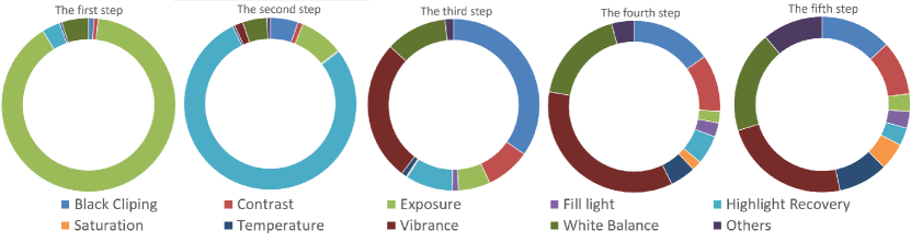
Figure 3: Retouching operations of artists in the dataset

2.3 Distribution of $ab$ values

As mentioned above, natural images in ImageNet are usually with low $ab$ values and desaturated. Similarly, we perform $ab$ values distribution analysis for all 5000 images of Expert C in MIT-Adobe FiveK, which are most commonly used as GT for retouching tasks. For each image, the first six major colors in the CIE Lab gamut (we use CIE Lab gamut for analysis because it is designed to approximate human visual perception) are extracted and analyzed. In this gamut, the values of $ab$ closer to 0 indicates the lower in saturation, while close to 1/ -1 indicate the higher saturation. L value indicates the luminance of the image, and the value of -1/ 1 represents the darkest/brightest the image.

As shown in Figure 4(e), scatters are main colors of GT, the colored spheres represent the range of the CIE lab gamut. The closer to the surface of the sphere, the higher the saturation is, while the distribution of the dataset is concentrated inside the sphere. Using the L=0, a=0, and b=0 planes to cut the color gamut, $ab$ values of GT concentrated in the area around a=0 and b=0, indicates that images have low saturation.

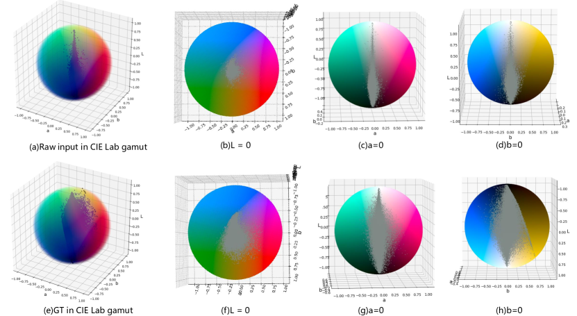
Figure 4: Distribution of raw images and GT images color values in CIE Lab color gamut

3 Method

In artful image retouching(AIR), common operations such as adjusting the exposure of highlights/ right hues/ dark hues/ shadows, or adjusting color temperature/hues by manipulating a global tone mapping curve only modify global features. Local operations using pixel-to-pixel color transformation are meticulous, which may cause degradation in spatial structures or inconsistent tone style in the local area. As mentioned above, we counted the first 500 images of artists’ retouching operations in the dataset. All 500 images used only global operations such as mapping curves. That is why LCCNet solely focuses on global operations and yields impressive results.

AIR is a cognitive task associated with personal aesthetics, not merely a signal processing problem like image super-resolution. The aesthetic evaluation of the image itself is vague, but artists can give a reason for their every operation in the process of retouching, such as "Hi, I think the background is too dark, I have to brighten it up". Therefore, not only should we focus on the retouched image, but also the retouching behavior should be considered. First, EXIF of photos, which has been ignored in previous methods is introduced. Secondly, the operation of artists’ manual retouching is concerned and imitated. Finally, rebalancing the color imbalance in the dataset. Based on the above analysis, the EXIF is used as condition input to improve the one-to-many color mapping problem. A two-stage network that cascade luminance and chrominance is designed. The hue palette loss is designed to solve the problem of uneven color distribution in the training dataset so that colors in an image get the same attention.

3.1 Prior knowledge-EXIF

It is natural to use EXIF for AIR to improve the automatic retouching algorithm since AIR is closely related to the image’s scene.

In [17; 16], they use condition vectors generated from image content to adjust feature maps globally. Similarly, we use the EXIF condition vector to generate adjustment coefficients and apply them to feature maps. Because the scene information is associated with the whole image, the adjustment coefficients are global, not local.

As shown in the Figure 5(b), the condition vector passes through a series of fully-connected layers to generate global adjustment coefficients, which are applied to the feature map of each layer.

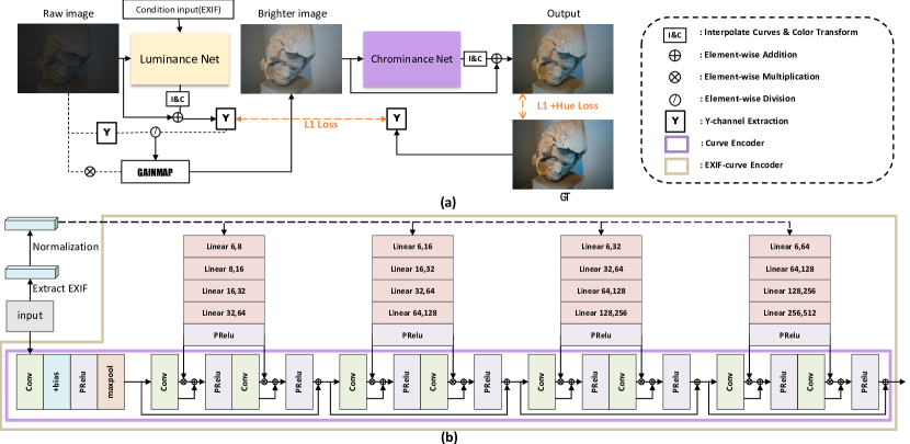
Figure 5: Main structure of LCCNet

3.2 Luminance-chrominance cascading structure

A cascaded two-stage network structure is obtained by simulating artists’ retouching operations based on the above analysis, which adjusts brightness first then chrominance. As shown in Figure 5(a), the first-stage network focuses on illumination improvement, and the second-stage network is used to enrich the color of the highlighted image generated by the first-stage network.

The luminance adjustment of the former stage network is implemented in the $YUV$ (BT601) color gamut. In this color gamut, the $Y$ channel indicates the luminance of the picture. The conversion between the $RGB$ color gamut and $YUV$ color gamut is linear. For input pixel $I(x,y)(I\in[0,1],x,y\in H\times W)$ in an image $I$ with $H\times W$ resolution, the conversion formula is as follows:

$$\left[\begin{array}[]{ccc}I(x,y)^{Y}\\ I(x,y)^{U}\\ I(x,y)^{V}\\ \end{array}\right]=\left[\begin{array}[]{ccc}0.299&0.587&0.114\\ -0.169&-0.331&0.5\\ 0.5&-0.419&-0.081\\ \end{array}\right]\left[\begin{array}[]{ccc}I(x,y)^{R}\\ I(x,y)^{G}\\ I(x,y)^{B}\\ \end{array}\right].$$ (1)

$Y^{\prime}$ indicates the luminance for whole image after brightness changes, and $gainmap$ can be expressed as $Y^{\prime}$ element-wise division by $Y$. Here the $gainmap$ is a matrix with the same height and width as the input image. Each element in the matrix independently adjusts the pixel value of the corresponding position. Using $gainmap$ element-wise multiplies $RGB$ input to obtain the $R^{\prime}G^{\prime}B^{\prime}$ after luminance adjustment.

Compared with the independent learning process in which all three $RGB$ channels are involved, using the same gain for each channel does not damage the proportion relationship of the three $RGB$ channels of the image itself, that is, the hue of the image. For the training process, this achieves luminance alignment without changing hue during adjustment.

The output of the first-stage network is used as the input of the second-stage network. Compared with the original input of low brightness, the brighter image input to the secondary network has a wider range of color gamut. In this case, the operation of chrominance becomes easier.

3.3 Hue palette loss

Using the Euclidean or L1 loss in photo retouching tends to average the set under a series of distinct $ab$ values, thus the colors occupying larger areas of the graph will be paid more attention and the smaller parts may be ignored. This is contrary to the usual cognition because it is not the part with the largest area in the image which attracts the most attention, but the part with a significantly different color from the surroundings that attracts people’s attention, no matter how small its area is. According to our analysis, the dataset presents a low ab value and low saturation distribution, thus using L1/L2 loss alone may ignore saturated portions with high ab values and inevitably lead to a less vibrant output.

Hue palette loss is designed to balance the attention of each color component to saturate the image more. As shown in Figure 6, first, the $RGB$ input is converted to the $HSV$ gamut, and then the $H$ channel is extracted because the $H$ channel is hue and represents the category of color contained in the image. The histogram of $H$ channel is exploited. In this histogram, too wide of bin width can cause color confusion, while too narrow will cause similar colors to be divided into different ranges. By measuring different interval widths and computational costs by experiment, we divide the H channels in the range of [0, 360] into 10 equal bins, each interval width is 36. More details of can be seen in supplementary material.

Each bin represents a color in the image and the position of each color in the image can be obtained by reversely searching for the coordinates of the corresponding pixel value in the image. The coordinate points in the image corresponding to the current color are assigned to 1; otherwise, the coordinates are assigned to 0. The Coordinate Mask is used to element-wise multiply input and the GT image. Hue loss for the corresponding color is obtained and normalized by using the number of pixels for the corresponding color to eliminate the impact of the area. The Hue palette loss is formulated below:

$$Hue\_palette\_loss =\sum_{j=1}^{k}Hue\_loss_{k} =\sum_{j=1}^{k}\frac{d_{1}(output*CM_{j},GT*CM_{j})}{SUM(CM_{j})}.$$ (2)

Here in Equation(2) $CM_{j}$ indicates the j-th of Coordinate Mask, and $*$ means Hadamard product. For two $m\times n$ matrices $A=[a_{ij}]$ and $B=[b_{ij}]$, $(A*B)_{ij}=a_{ij}b_{ij}$, $d_{1}(A,B)=\sum_{i=1}^{n}\sum_{j=1}^{n}|a_{ij}-b_{ij}|$, $SUM(A)=\sum\sum a_{ij}$.

Hue palette loss eliminates the influence of the color area by normalizing the number of pixels corresponding to the color and colors of different areas get the same attention. In this way, imbalances in the dataset due to low $ab$ values are resolved and the images are more saturated.

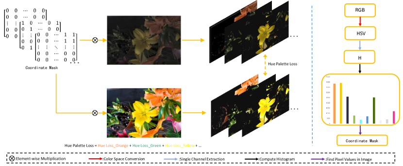
Figure 6: The generation mode of Hue palette loss. All graphs are real calculation processes, and the color of the histogram is the corresponding color in the original image.

4 Experiments and implementation details

4.1 Dataset and Metrics

MIT-Adobe FiveK dataset is a commonly-used photo retouching dataset that consists of 5,000 raw photographs taken with SLR cameras. All these photographs have been retouched by five retouching experts (A/B/C/D/E). Following the previous methods  [17; 41; 10; 33; 21; 38; 29; 9; 32] to use the retouched results of expert C(sRGB color gamut) as the ground truth (GT), and adopting the same pre-processing procedures as  [17; 40; 30] that all the images are resized to 500px on the long edge for training. The images of the default input style as input are used, and the first 4500 image pairs are used for training and the last 500 image pairs for testing. PSNR, SSIM, and LPIPS [28] are used to evaluate the performance of all methods.

4.2 LCCNet

The curve approach in [41], named basic enhancer is applied as the basic model in LCCNet. The basic enhancer assumes that each channel of the output image is correlated with each channel of the input image as well as the coordinate maps ${x,y}$ of each image. We used the simple form of the basic enhancer, where the output channels related to the coordinate maps ${x,y}$ are affected by the image size but independent of the input pixel values. We implemented LCCNet using the pytorch framework [3]. LCCNet is a two-stage network, images with EXIF(Very few images contain some but not all of the six pieces of information. For information not included in the EXIF, we chose to set it to 0.) are input to the network together. The $Y^{\prime}$ channel generated after the Brighter Net training uses the L1 loss to fit the $Y$ channel of the GT image. $Gainmap$ is applied to the original input by multiplying the element direction to generate a highlight image for Richer Color Net. Hue palette loss and L1 loss under the CIE-Lab gamut are used for the final output with the same weight.

4.3 Comparison with State-of-the-Arts

LCCNet is trained on a single NVIDIA V100 for 2000 epochs with a batch of 32 for 15h. In addition, the random seed is set to 6 to ensure that the result can be reproduced. LCCNet is compared with contemporaneous methods on MIT-Adobe FiveK as shown in Table1. HDRNet, DPE, DUPE, DeepLPF are local based method. CURL, STAREnhancer and our method are globaled based and use curve-based approachs. A3D-LUT and AdaInt are both tabel-based and CSRNet use condition vector generated from images for global retouching. LCCNet achieves optimal PSNR and SSIM in both low and original resolution. At the same time, the best SSIM is in low resolution and the second in high resolution. Moreover, because our method is a global adjustment, the effect is stable with resolution varying.

Table 1: Quantitative comparison with contemporaneous methods on MIT-Adobe-FiveK. Red figure indicates the best and Blue indicates the second best. Note that for underlined methods we retrained them, and for other methods we use the result in their origin paper (some are absent (“/”) for lacking of source code).

		480P			Full resolution
Method	PSNR(↑)	SSIM(↑)	LPIPS(↓)	PSNR(↑)	SSIM(↑)	LPIPS(↓)
HDRNet [21]	24.66dB	0.915	0.076	23.20dB	0.917	0.120
DPE [39]	23.75dB	0.908	/	22.15dB	0.850	/
DeepUPE [29]	/	/	/	23.24dB	0.893	0.158
DeepLPF [32]	23.93dB	0.903	0.582	24.48dB	0.887	0.103
CSRNet[17]	25.14dB	0.924	0.062	24.82dB	0.926	0.091
A3D-LUT [9]	25.50dB	0.890	0.051	23.17dB	0.864	0.145
CURL [33]	/	/	/	24.20dB	0.880	0.108
STAREnhancer[41]	25.40dB	0.939	0.044	25.46dB	0.948	0.083
AdaInt [38]	25.49dB	0.926	/	25.48dB	0.934	/
LCCNet	25.81dB	0.944	0.041	25.80dB	0.947	0.074

Figure7 shows some of the test images. Thanks to the design of the luminance network, in the first scene LCCNet’s luminance is closest to the real scene. In addition, LCCNet also performs well for the red color in a small area thanks to hue palette loss. The second scenario has a lot of interlaced details, and our method successfully focuses on each area compared to other methods. Please see the supplementary for more comparisons.

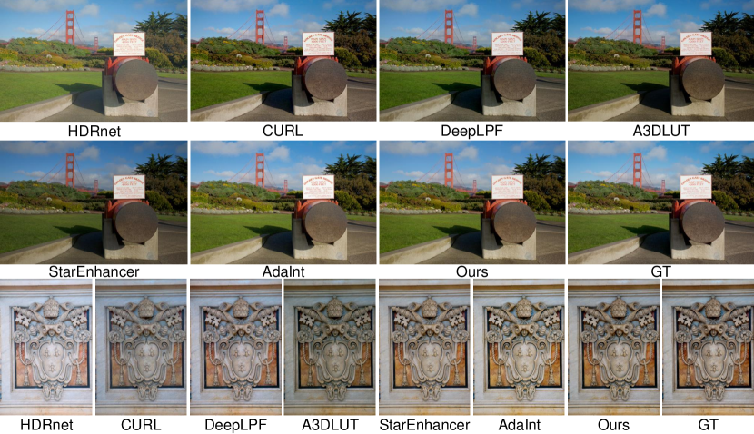
Figure 7: Qualitative comparison with contemporaneous methods on MIT-Adobe fiveK.

4.4 Ablation study

To demonstrate the effectiveness of different components of LCCNet, several ablation studies are conducted on the MIT-fiveK dataset. As shown in Table2, each component in LCCNet can independently improve the performance of the basic model and work together.

Noting that using our proposed $gainmap$ structure performs better than directly cascading two basic models, because the two networks perform their own independent functions. As shown in the top row of Figure 8 it’s obvious that the clothes generated by basic model is darker. Using the extracted from GT and raw images, then apply them to raw inputs. The brighter images gain from $gainmaps$ inputted to basic model can achieve a highly 29.79 dB of PSNR. It can be seen that after adjusting the brightness to the appropriate range, the subsequent color processing is easier and more effective. In the second row in Figure 8, EXIF is used to map colors correctly and green is closer to the grass in nature. In addition, since CSRNet [17] is a typical method that uses condition input for image retouching, we apply EXIF as a condition input to CSRNet in the same way as LCCNet, and Table 3 shows a steady increase in PSNR and SSIM at the cost of very few parameters. Details of the experiments and comparisons of the effects are provided in the supplementary materials.

Hue palette loss is designed to focus on fewer colors in unbalanced datasets, in the last row of Figure 8, the white arm position is not affected by a dark background, and the blue saturation of the sky is higher and closer to reality.

Table 2: Different components of LCCNet(480P)

Method	basic model	basic-EXIF	basic-two stage	basic-basic	basic-hue loss	LCCNet
PSNR(↑)	25.40dB	25.73dB	25.72dB	25.58dB	25.69dB	25.81dB
SSIM(↑)	0.939	0.939	0.942	0.940	0.941	0.943

Table 3: original CSRNet and CSRNet-EXIF

Method	PSNR(↑)	SSIM(↑)	Parameters(↓)
CSRNet	23.69dB	0.895	36489
CSRNet-EXIF	23.94dB	0.896	37406

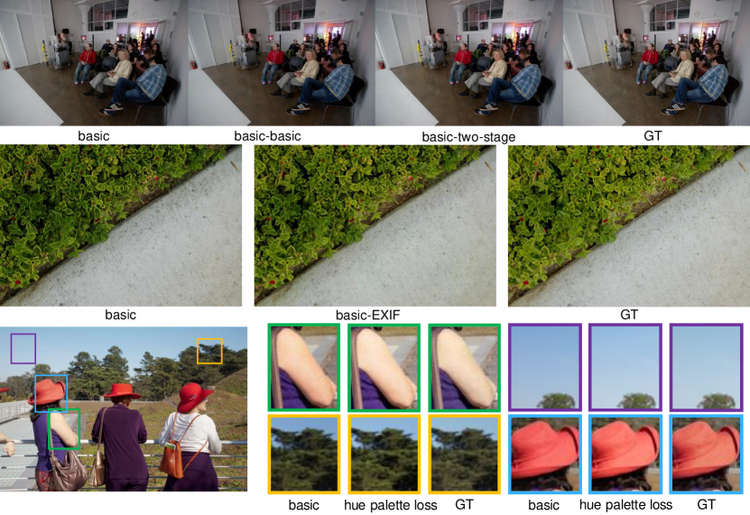
Figure 8: The effect of basic model and adding different modules that we proposed.

5 Conclusion

In this paper, we propose LCCNet which focuses more on artists’ operations and achieve state-of-art performance on the MIT-Adobe-FiveK. We add EXIF to an automated retouching network, which proves its effectiveness on LCCNet and CSRNet. At the same time, the luminance-chrominance decoupling of humanoid operations is effective. Finally, a balanced hue palette loss for solving the imbalance in the training dataset is proposed. Noting that our approach is generic and therefore can be extended to other methods.

There is still room for further experimental optimizations of the optimal EXIF information combination. A two-stage network brings more computational cost compared with benefits, a better way of cascading need further research.

6 Appendix

6.1 EXIF in CSRNet

In LCCNet, EXIF has been proven to work in AIR, and naturally, it can also be added to other auto retouching networks to make the output more in line with human aesthetics. In this section, EXIF is added to CSRNet[17]. Similarly, a noticeable improvement in the same condition as their paper set is got.

CSRNet consists of a base network and a condition network, and it uses global coefficients obtained from conditional networks to modulate the intermediate features. As shown in the Figure 9(a), since CSRNet regards image’s content as a condition vector, the scene information contained in the EXIF can also be used as a condition vector. A global adjustment coefficient $c$ generated by EXIF is added to the original CSRNet affine transformation.

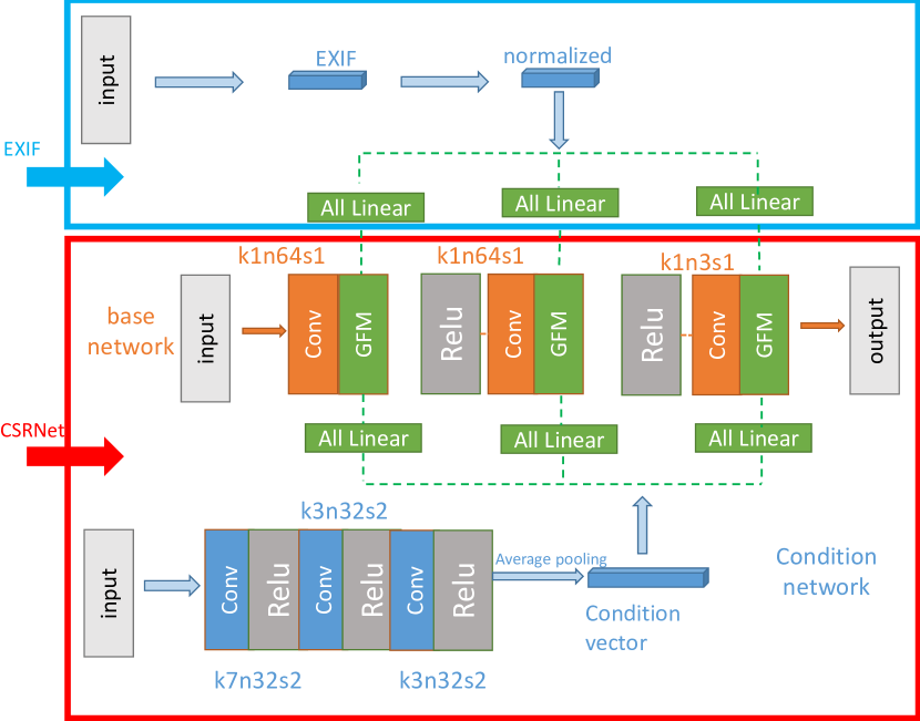
(a) Main Structure of CSRNet and Method of Adding EXIF

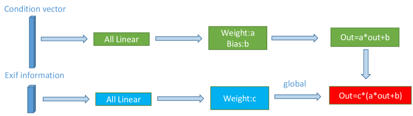
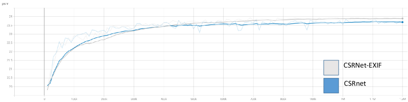
(b) EXIF Generating Global Coefficient $c$

(c) EXIF Test Set PSNR Curves for CSRNet and CSRNet-EXIF (after smoothing).

Figure 9: Original CSRNet and CSRNet-EXIF

Table 4: original CSRNet and CSRNet-EXIF

Method	PSNR	SSIM	FPS	Parameters
CSRNet	23.69dB	0.895	12.9	36489
CSRNet-EXIF	23.94dB	0.896	13.5	37406

Under the same training parameters and dataset partitioning method as CSRNet (the dataset paper released is used), the introduced prior knowledge increases 2.5% of parameters, increases 0.24 dB PSNR stably, decreases 5.1% MSE, and accelerates the inference speed of the model. Although the number of network parameters is slightly increased, the inference process is easier for the network due to the increase of effective information, which accelerates the inference process of the network. The curve in the Figure 9(c) shows that the PSNR increases stably in the test set. And Figure10 shows that the introduction of EXIF priori knowledge significantly improved the color effect of some scenes on CSRNet that are strongly related to the scene information.

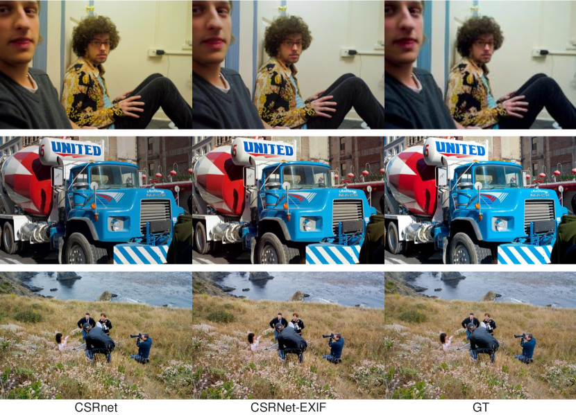
Figure 10: Qualitative comparison between CSRNet and CSRNet-EXIF.

The six-dimensional vector used is $[ISO,Exposure,Fnumber,Speed,Flength,Biasvalue]$, the average of the six-dimensional vector full dataset and the average of the training set are respectively $[456.131,0.2423,6.4261,7.0484,55.9858,0.02]$ and $[441.23,0.258,6.4664,7.0714,56.6272,0.018]$. In order to make the influence of each dimension the same, $[iso/1000.0,expotime*1000,fnumber,speed,flength/10.0,biasvalue]$ is used for normalization.

6.2 Details of the Artist’s Operations

A pie chart is used in the main paper to show the proportion of the artist’s retouching operations, and the detailed operation data is in Table5. The artist’s operation is obtained from the lightroom of the original dataset, and the operation steps of a single image in lightroom are shown in Figure 11.

Table 5: The specific statistics of the artist’s operations, the total number of operations in the last two steps is less than 500 because the operation steps of some pictures are less than 5 steps. Operations not involved are marked as (“/”).

Operations	The first step	The second step	The third step	The fourth step	The fifth step
Black Clipping	5	26	174	75	60
Brightness	/	1	/	6	6
Contrast	4	5	42	53	46
Dark Tones	/	1	2	7	15
Exposure	447	41	30	11	15
Fill light	/	1	6	13	14
Highlight Recovery	17	391	41	27	15
Light Tones	/	/	/	2	13
Midtone Split	/	/	/	/	1
Highlight Tones	/	/	/	/	4
Saturation	/	/	1	9	23
Shadow Tones	/	/	1	1	5
Temperature	2	2	5	24	42
Tint	/	1	4	5	7
Vibrance	/	8	133	173	108
White Balance	25	23	60	89	86
Total	500	500	500	495	460

Figure 11: The artist’s retouching operations in a single image, the software is Lightroom.

6.3 Hue Palette Loss Implementation Details

The hue palette loss designed needs to specify the number of divided histogram intervals, that is, the number of classes of colors. The influence of the number of different intervals on the final LCCNet results is shown in the table. In this histogram, too wide of bin width can cause color confusion, while too narrow will cause similar colors to be divided into different ranges. We divide the H channels in the range of [0, 360] into 10 equal bins by experiments. For a single image 12, the ten colors after extraction are shown in Figure 13.

Table 6: The Effect of the Number of Colors on Hue Loss(480P).

number of intervals	5	6	8	9	10	12	20	30
PSNR	25.74dB	25.69dB	25.68dB	25.77dB	25.81dB	25.68dB	25.70dB	25.68dB

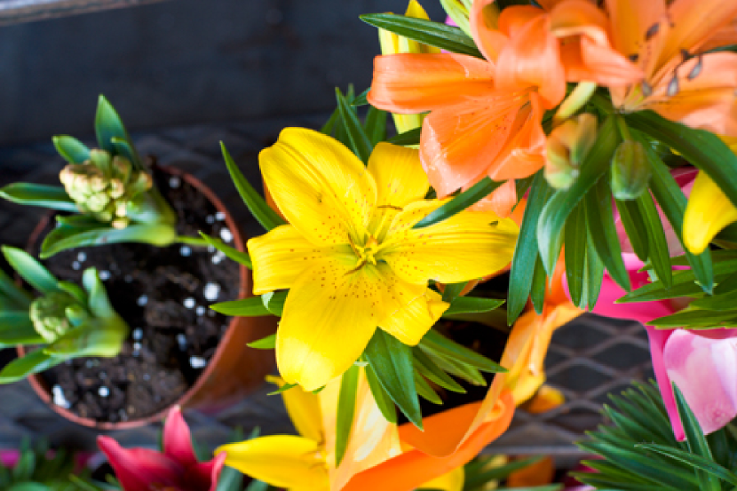
Figure 12: The 959th image in the MIT Adobe-fiveK dataset

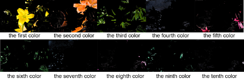
Figure 13: Ten Colors Extracted

6.4 Qualitative comparison of LCCNet Modules

We conducted experiments on the effects of each module in LCCNet. Figure 14 shows the comparison results of basic model and basic model-EXIF, the addition of EXIF makes the image closer to GT in chrominance. Figure 15 shows the comparison results of basic model and basic model-two stage, in addition, the simple cascaded form basic-basic without $gainmap$ is also compared. The structure of the two stage makes the luminance more realistic. Figure 16 shows the comparison results of basic model and basic model-hue palette loss. It can be seen from the clothes that the hue loss that added make the color more saturated.

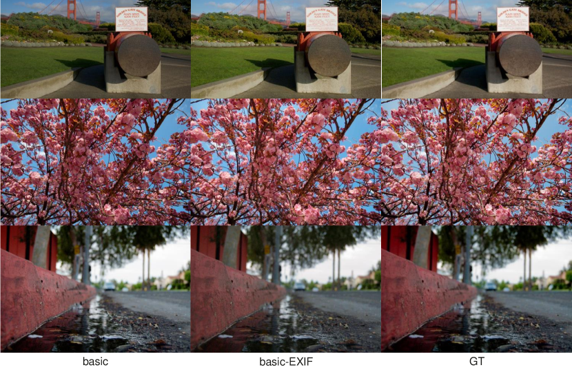
Figure 14: Qualitative Comparison Between Basic Model and Basic Model-EXIF.

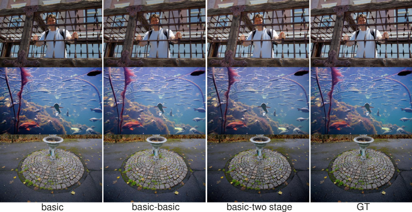
Figure 15: Qualitative Comparison Between Basic Model and Basic Model-two stage.

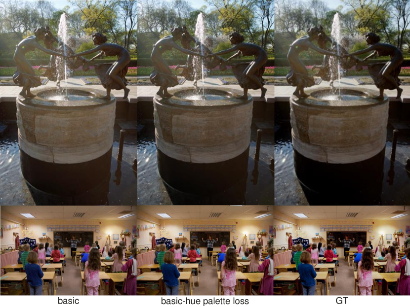
Figure 16: Qualitative Comparison Between Basic Model and Basic Model-hue palette loss.

6.5 Additional Comparison with Contemporaneous Methods

An additional comparison methods with the contemporaneous method, including HDRNet [21], CURL [33], DeepLPF [32], A3D-LUT [9], StarEnhancer [41], AdaInt [38]. The results can be seen in Figure 17, Figure 18 and Figure 19. In Figure 17, our method closer to GT in chrominance, and the second scene has the closest brightness performance to the reality. In Figure 18, our sky color is the most realistic, the foreground and background of the stone statue are close to GT. In Figure 19 both the flowers in the first scene and the grass in the second are more realistic in chrominance, at the same time, the deviation between the brightness and the real scene is small.

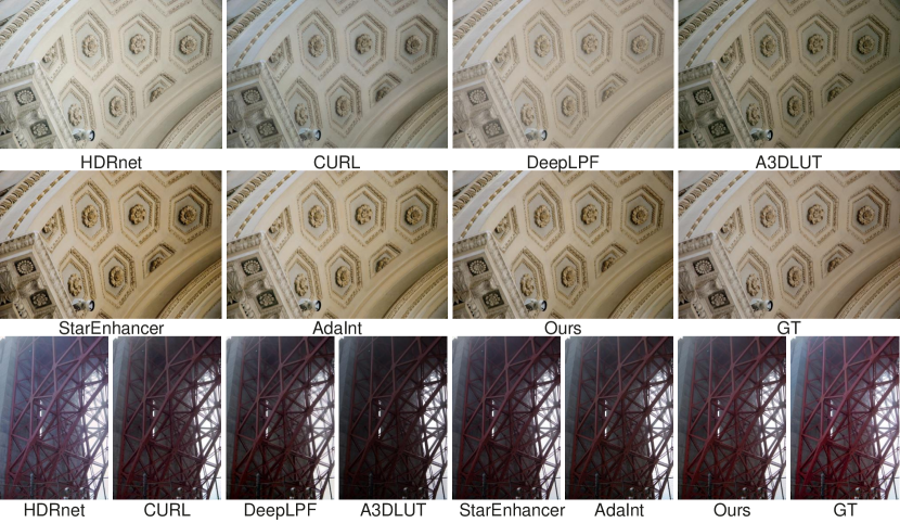
Figure 17: Qualitative Comparison with Contemporaneous Methods on MIT-Adobe fiveK.

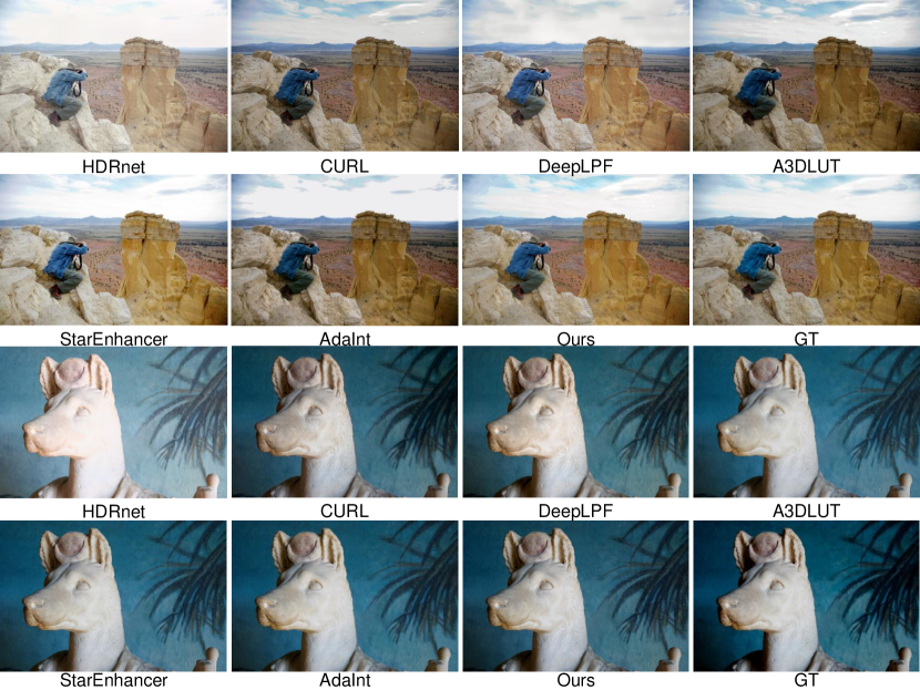
Figure 18: Qualitative Comparison with Contemporaneous Methods on MIT-Adobe fiveK.

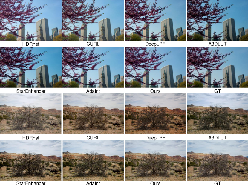
Figure 19: Qualitative Comparison with Contemporaneous Methods on MIT-Adobe fiveK.

References

- [1] https://www.adobe.com/products/photoshop.html.
- [2] https://www.adobe.com/products/photoshop-lightroom.html.
- [3] Paszke Adam, Gross Sam, Massa Francisco, Lerer Adam, Bradbury James, Chanan Gregory, Killeen Trevor, Lin Zeming, Gimelshein Natalia, Antiga Luca, Desmaison Alban, Kopf Andreas, Yang Edward, DeVito Zachary, Raison Martin, Tejani Alykhan, Chilamkurthy Sasank, Steiner Benoit, Fang Lu, Bai Junjie, and Chintala Soumith. Pytorch: An imperative style, high-performance deep learning library. In H. Wallach, H. Larochelle, A. Beygelzimer, F. d'Alché-Buc, E. Fox, and R. Garnett, editors, Advances in Neural Information Processing Systems, volume 32. Curran Associates, Inc., 2019.
- [4] Vladimir Bychkovsky, Sylvain Paris, Eric Chan, and Frédo Durand. Learning photographic global tonal adjustment with a database of input / output image pairs. In The Twenty-Fourth IEEE Conference on Computer Vision and Pattern Recognition, 2011.
- [5] Guo Chunle, Li Chongyi, Guo Jichang, Loy Chen Change, Hou Junhui, Kwong Sam, and Cong Runmin. Zero-reference deep curve estimation for low-light image enhancement. In Proceedings of the IEEE/CVF Conference on Computer Vision and Pattern Recognition (CVPR), June 2020.
- [6] Jiang Duan and Guping Qiu. Novel histogram processing for colour image enhancement. In Third International Conference on Image and Graphics (ICIG’04), pages 55–58, 2004.
- [7] Durand F. Fast bilateral filtering for the display of high-dynamic-ranges images. Siggraph, 2002.
- [8] Finlayson G. D. and E. Trezzi. Shades of gray and colour constancy. pages 37–41, Nov. 2004. 12th Color Imaging Conference: Color Science and Engineering Systems, Technologies, and Applications ; Conference date: 01-11-2004.
- [9] Zeng H., Cai J., Li L., Cao Z., and Zhang L. Learning image-adaptive 3d lookup tables for high performance photo enhancement in real-time. IEEE Transactions on Software Engineering, PP, 2020.
- [10] Kim Han-Ul, Koh Young Jun, and Kim Chang-Su. Global and local enhancement networks for paired and unpaired image enhancement. In Vedaldi Andrea, Bischof Horst, Brox Thomas, and Frahm Jan-Michael, editors, Computer Vision – ECCV 2020, pages 339–354, Cham, 2020. Springer International Publishing.
- [11] Kim Hanul, Choi Su-Min, Kim Chang-Su, and Koh Yeong Jun. Representative color transform for image enhancement. In Proceedings of the IEEE/CVF International Conference on Computer Vision (ICCV), pages 4459–4468, October 2021.
- [12] Xu Hongteng, Zhai Guangtao, Wu Xiaolin, and Yang Xiaokang. Generalized equalization model for image enhancement. IEEE Transactions on Multimedia, 16(1):68–82, 2014.
- [13] Stark J.A. Adaptive image contrast enhancement using generalizations of histogram equalization. IEEE Transactions on Image Processing, 9(5):889–896, 2000.
- [14] Liang Jie, Zeng Hui, and Zhang Lei. High-resolution photorealistic image translation in real-time: A laplacian pyramid translation network. In Proceedings of the IEEE/CVF Conference on Computer Vision and Pattern Recognition (CVPR), pages 9392–9400, June 2021.
- [15] Shi Jing, Xu Ning, Xu Yihang, Bui Trung, Dernoncourt Franck, and Xu Chenliang. Learning by planning: Language-guided global image editing. In Proceedings of the IEEE/CVF Conference on Computer Vision and Pattern Recognition (CVPR), pages 13590–13599, June 2021.
- [16] He Jingwen, Dong Chao, and Qiao Yu. Interactive multi-dimension modulation with dynamic controllable residual learning for image restoration. In Vedaldi Andrea, Bischof Horst, Brox Thomas, and Frahm Jan-Michael, editors, Computer Vision – ECCV 2020, pages 53–68, Cham, 2020. Springer International Publishing.
- [17] He Jingwen, Liu Yihao, Qiao Yu, and Dong Chao. Conditional sequential modulation for efficient global image retouching. In Vedaldi Andrea, Bischof Horst, Brox Thomas, and Frahm Jan-Michael, editors, Computer Vision – ECCV 2020, pages 679–695, Cham, 2020. Springer International Publishing.
- [18] Park Jongchan, Lee Joon-Young, Yoo Donggeun, and Kweon In So. Distort-and-recover: Color enhancement using deep reinforcement learning. In Proceedings of the IEEE Conference on Computer Vision and Pattern Recognition (CVPR), June 2018.
- [19] Zhao Lin, Lu Shao-Ping, Chen Tao, Yang Zhenglu, and Shamir Ariel. Deep symmetric network for underexposed image enhancement with recurrent attentional learning. In Proceedings of the IEEE/CVF International Conference on Computer Vision (ICCV), pages 12075–12084, October 2021.
- [20] Aubry Mathieu, Paris Sylvain, Hasinoff Samuel W., Kautz Jan, and Durand Fredo. Fast local laplacian filters: Theory and applications. Acm Transactions on Graphics, 33(5):1–14, 2014.
- [21] Gharbi Michaël, Chen Jiawen, Barron Jonathan T., Hasinoff Samuel W., and Durand Frédo. Deep bilateral learning for real-time image enhancement. ACM Trans. Graph., 36(4), jul 2017.
- [22] S.K. Naik and C.A. Murthy. Hue-preserving color image enhancement without gamut problem. IEEE Transactions on Image Processing, 12(12):1591–1598, 2003.
- [23] Russakovsky O., Deng J., Su H., Krause J., Satheesh S., Ma S., Huang Z., Karpathy A., Khosla A., and Bernstein M. Imagenet large scale visual recognition challenge. International Journal of Computer Vision, 115(3):211–252, 2015.
- [24] Isola Phillip, Zhu Jun-Yan, Zhou Tinghui, and Efros Alexei A. Image-to-image translation with conditional adversarial networks. In 2017 IEEE Conference on Computer Vision and Pattern Recognition (CVPR), pages 5967–5976, 2017.
- [25] Gao Qifan and Wu Xiaolin. Real-time deep image retouching based on learnt semantics dependent global transforms. IEEE Transactions on Image Processing, 30:7378–7390, 2021.
- [26] Dahl R. Automatic colorization. 2016.
- [27] Zhang R. and Isola P.and Efros A.A. Colorful image colorization. European Conference on Computer Vision, 9907:649–666, 2016.
- [28] Zhang Richard, Isola Phillip, Efros Alexei A., Shechtman Eli, and Oliver Wang. The unreasonable effectiveness of deep features as a perceptual metric. In Proceedings of the IEEE Conference on Computer Vision and Pattern Recognition (CVPR), June 2018.
- [29] Wang Ruixing, Zhang Qing, Fu Chi-Wing, Shen Xiaoyong, Zheng Wei-Shi, and Jia Jiaya. Underexposed photo enhancement using deep illumination estimation. In Proceedings of the IEEE/CVF Conference on Computer Vision and Pattern Recognition (CVPR), June 2019.
- [30] Yu Runsheng, Liu Wenyu, Zhang Yasen, Qu Zhi, Zhao Deli, and Zhang Bo. Deepexposure: Learning to expose photos with asynchronously reinforced adversarial learning. In S. Bengio, H. Wallach, H. Larochelle, K. Grauman, N. Cesa-Bianchi, and R. Garnett, editors, Advances in Neural Information Processing Systems, volume 31. Curran Associates, Inc., 2018.
- [31] Agaian Sos S., Silver Blair, and Panetta Karen A. Transform coefficient histogram-based image enhancement algorithms using contrast entropy. IEEE Transactions on Image Processing, 16(3):741–758, 2007.
- [32] Moran Sean, Marza Pierre, McDonagh Steven, Parisot Sarah, and Slabaugh Gregory. Deeplpf: Deep local parametric filters for image enhancement. In Proceedings of the IEEE/CVF Conference on Computer Vision and Pattern Recognition (CVPR), June 2020.
- [33] Moran Sean, McDonagh Steven, and Slabaugh Gregory. Curl: Neural curve layers for global image enhancement. In 2020 25th International Conference on Pattern Recognition (ICPR), pages 9796–9803, 2021.
- [34] Wang Tao, Li Yong, Peng Jingyang, Ma Yipeng, Wang Xian, Song Fenglong, and Yan Youliang. Real-time image enhancer via learnable spatial-aware 3d lookup tables. In Proceedings of the IEEE/CVF International Conference on Computer Vision (ICCV), pages 2471–2480, October 2021.
- [35] Arici Tarik, Dikbas Salih, and Altunbasak Yucel. A histogram modification framework and its application for image contrast enhancement. IEEE Transactions on Image Processing, 18(9):1921–1935, 2009.
- [36] Xinxu Wei, Xianshi Zhang, Shisen Wang, Yanlin Huang, and Yongjie Li. Tsn-ca: A two-stage network with channel attention for low-light image enhancement. arXiv preprint arXiv::2110.02477v1, 2021.
- [37] Zhicheng Yan, Hao Zhang, Baoyuan Wang, Sylvain Paris, and Yizhou Yu. Automatic photo adjustment using deep neural networks. ACM Trans. Graph., 35(2), feb 2016.
- [38] Canqian Yang, Meiguang Jin, Xu Jia, Yi Xu, and Ying Chen. Adaint: Learning adaptive intervals for 3d lookup tables on real-time image enhancement. 2022 IEEE Conference on Computer Vision and Pattern Recognition (CVPR), 2022.
- [39] Chen Yu-Sheng, Wang Yu-Ching, Kao Man-Hsin, and Chuang Yung-Yu. Deep photo enhancer: Unpaired learning for image enhancement from photographs with gans. In Proceedings of the IEEE Conference on Computer Vision and Pattern Recognition (CVPR), June 2018.
- [40] Hu Yuanming, He Hao, Xu Chenxi, Wang Baoyuan, and Lin Stephen. Exposure: A white-box photo post-processing framework. ACM Transactions on Graphics, 37(2), may 2018.
- [41] Song Yuda, Qian Hui, and Du Xin. Starenhancer: Learning real-time and style-aware image enhancement. In Proceedings of the IEEE/CVF International Conference on Computer Vision (ICCV), pages 4126–4135, October 2021.
- [42] Cheng Zezhou, Yang Qingxiong, and Sheng Bin. Deep colorization. In Proceedings of the IEEE International Conference on Computer Vision (ICCV), December 2015.
- [43] Pan Zhaoqing, Yuan Feng, Lei Jianjun, Li Wanqing, Ling Nam, and Kwong Sam. Miegan: Mobile image enhancement via a multi-module cascade neural network. IEEE Transactions on Multimedia, 24:519–533, 2022.
- [44] Zhang Zhaoyang, Jiang Yitong, Jiang Jun, Wang Xiaogang, Luo Ping, and Gu Jinwei. Star: A structure-aware lightweight transformer for real-time image enhancement. In Proceedings of the IEEE/CVF International Conference on Computer Vision (ICCV), pages 4106–4115, October 2021.