Accelerated Primal-Dual Mirror Dynamics for Centrailized and Distributed Constrained Convex Optimization Problems
Abstract
This paper investigates two accelerated primal-dual mirror dynamical approaches for smooth and nonsmooth convex optimization problems with affine and closed, convex set constraints. In the smooth case, an accelerated primal-dual mirror dynamical approach (APDMD) based on accelerated mirror descent and primal-dual framework is proposed and accelerated convergence properties of primal-dual gap, feasibility measure and the objective function value along with trajectories of APDMD are derived by the Lyapunov analysis method. Then, we extend APDMD into two distributed dynamical approaches to deal with two types of distributed smooth optimization problems, i.e., distributed constrained consensus problem (DCCP) and distributed extended monotropic optimization (DEMO) with accelerated convergence guarantees. Moreover, in the nonsmooth case, we propose a smoothing accelerated primal-dual mirror dynamical approach (SAPDMD) with the help of smoothing approximation technique and the above APDMD. We further also prove that primal-dual gap, objective function value and feasibility measure of SAPDMD have the same accelerated convergence properties as APDMD by choosing the appropriate smooth approximation parameters. Later, we propose two smoothing accelerated distributed dynamical approaches to deal with nonsmooth DEMO and DCCP to obtain accelerated and efficient solutions. Finally, numerical experiments are given to demonstrate the effectiveness of the proposed accelerated mirror dynamical approaches.
Keywords: machine learning, accelerated mirror dynamical approaches, smooth and nonsmooth optimization, constrained optimization, smoothing approximation, distributed approaches
1 Introduction
1.1 Problem statement
In this paper, we consider the following convex constrained optimization problem:
| (1) |
where
| (2) |
This problem covers many optimization problems in various applied fields such as machine learning, sparse signal reconstruction, image deblurring, resource allocation, saddle point, Markov decision processes, regularized empirical risk minimization, and supervised machine learning. (see, e.g. Boyd et al. (2011); Lin et al. (2020); Darbon and Langlois (2021); O’Connor and Vandenberghe (2014); Nandwani et al. (2019); Zhang and Xiao (2017); Tiapkin and Gasnikov (2022)).
1.2 Historical presentation
The inertial (scend-order or accelerated) dynamical approaches are increasingly popular for solving the unconstrained optimization problem
| (3) |
To deal with problem (3), Polyak (1964) first proposed the heavy ball with friction dynamical approach
| (4) |
where is a damping parameter. Later, Alvarez (2000) studied the asymptotic behavior of (4) with a time independent parameter when is convex. Bégout et al. (2015) studied some convergence properties of the HBF (4) with a constant when is a nonconvex function. Aujol et al. (2022, 2020) investigated the convergence rate of HBF dynamical system and its corresponding discrete algorithm with a fixed parameter under the condition that satisfies quasi-strongly convex and Lojasiewicz properties, respectively. Su et al. (2016) first revealed that the HBF (4) with can be regarded as the continuous-time limit of the Nesterov’s accelerated gradient algorithm and it has an accelerated convergence rate, i.e, . Elloumi et al. (2017) further improved the convergence rate of it to . When , the convergence rate was estimated by Attouch et al. (2019) and Apidopoulos et al. (2018) for smooth and nonsmooth convex functions . Cabot and Frankel (2012) studied the asymptotic behavior of the HBF (4) when . Moreover, Wibisono et al. (2016) studied a series of accelerated (inertial) dynamical approaches to the problem (3) by the Bregman Lagrangian based on the calculus of variations. Kovachki and Stuart (2021) studied the behavior of momentum methods for solving problem (3) from a continuous-time perspective. Wilson et al. (2021) proposed several Lyapunov functions for analyzing the accelerated (momentum) algorithms to solve the problem (3). By the manifold with curvature bounded from below, Alimisis et al. (2020) proposed a Riemannian variant of accelerated gradient dynamical approach.
Recently, to solve the problem (3) with a closed and convex set constraint , i.e.,
| (5) |
many inertial dynamical approaches have been studied. Based on the projection operators, He et al. (2016) proposed an inertial dynamical approach to solve the problem (5) with non-convex objective functions. Later, based on the work in He et al. (2016) and smoothing approximation technique, two smoothing inertial hydrodynamic approaches were proposed to solve constrained nonconvx minimization problem to reconstruct the sparse signal in Zhao et al. (2018). Combining the dynamical approach of mirror descent with the continuous version of Nesterov’s acceleration algorithm, Krichene et al. (2015) proposed an accelerated mirror dynamical approach for problem (5) as follows:
| (6) |
where and is the gradient of conjugate of (see (2.3) ).
In addition, in order to solve the problem (3) with an affine constraint, i.e,
| (7) |
many inertial dynamical approaches under primal-dual framework were extensively investigated. Zeng et al. (2022) first proposed a second-order dynamical primal-dual approach for solving the problem (7) and proved that the convergence rate of the gap between the Lagrangian function and its optimal value is . The corresponding inertial dynamical approach is then extended to solve the distributed optimization problems. Later, Boţ and Nguyen (2021) improved the convergence rates of the works in Zeng et al. (2022) and provided the weakly convergence analysis to a primal-dual optimal solution of the problem (7). He et al. (2021) studied an inertial primal-dual dynamical approach without/with perturbations for separable convex optimization problems with an affine constraint. Attouch et al. (2021) proposed a temporally rescaled inertial augmented Lagrangian system (TRIALS) with three time-varying parameters (i.e., viscous damping, extrapolation and temporal scaling) to address separable smooth/nonsmooth convex optimization problems with an affine constraint, and presented the fast convergence properties of TRIALS. In addition, Luo (2021) further proposed a “second-order”+“first-order” primal-dual dynamical approaches for solving problem (7) with accelerated convergence guarantees.
However, many practical problems in machine learning, sparse signal reconstruction, image deblurring, resource allocation and so on , not only have affine constraints, but also have set constraints, as in problem (1). The problem (1) can be regarded as a generalization for the problems (3), (5), (7), (12) and (13). In recent years, some first order dynamical approaches based on primal-dual framework and projection were proposed by Liu et al. (2017); Qu and Li (2019); Yi et al. (2016); Zeng et al. (2018) to solve the problem (1) only with convergence analysis or ergodic convergence rate. To the best of our knowledge, accelerated (inertial) dynamical approaches based on primal-dual framework with non-ergodic convergence rates are rarely involved. It is worth noting that the inertial dynamical approaches mentioned above were used for solving the problems (3), (5) and (7) and they cannot be used directly for the problem (1).
This paper aims to investigate accelerated primal-dual dynamical approaches based on mirror descent and smoothing approximation methods for solving problem (1) with an accelerated non-ergodic convergence rate . Our contributions are summarized as follows:
-
•
For the problem (1) in the smooth case, an accelerated primal-dual mirror dynamical approach (APDMD) is proposed for the first time, it is used to solve problem (1) with accelerated convergence rates of Lagrangian and objective functions? gaps. We provide an interpretation of the APDMD from different perspectives (i.e., neurodynamic approach, Hamilton’s system, game theory and control theory). Moreover, based on the properties of conjugate function and Cauchy-Lipschitz-Picard theorem, the feasibility (i.e, ensuring that the trajectories of solutions always satisfy the set constraint), existence and uniqueness of the global solution of APDMD are obtained. Last, applying the APDMD to DCCP and EDMO leads to two distributed APDMDs (ADPDMD and ADMD) with accelerated convergence guarantees.
-
•
For the problem (1) in the nonsmooth case, a smoothing accelerated primal-dual mirror dynamical approach (SAPDMD) for the problem (1) is also proposed based on the smoothing approximation technique and APDMD, and it has accelerated convergence rates of Lagrangian and objective function gaps. We provide a comparative explanation between SAPDMD and state-of-the-art dynamical approaches besed on differential inclusion, Moreau-Yosida regularization and directional derivative methods. Moreover, we further analyze the convergence properties of SAPSMD and provide smooth parameter selection condition. Last, applying the SAPDMD to DCCP and EDMO leads to two distributed SAPDMDs (SADPDMD and SADMD) with accelerated convergence gurantees.
- •
The paper is organized as follows. Section 2 introduces some preliminaries of convex analysis, saddle point theorem, dual distance, Bregman divergence, projection operators, graph theory and smoothing approximation. Then, we propose the APDMD to solve problem (1) in the smooth case, and discuss some convergence properties of APDMD in Section 3. In Section 4, we propose a SAPDMD (smoothing version of APDMD) for solving the problem (1) in the nonsmooth case, and provide a detailed discussion of the convergence properties of SAPDMD and then extend the SAPDMD to address the DCCP and EDMO in the nonsmooth case. Section 5 provides several experiments to demonstrate the theoretical results. Finally, we conclude this paper in Section 6.
2 Preliminaries
This section gives some essential mathematical preliminaries.
2.1 Convex analysis
A function is convex, if it satisfies , and . The subdifferential of with respect to is defined by , and the element of is called subgradient of . In addition, if is smooth, the subgradient reduces to gradient .
2.2 Saddle point Theorem
2.3 Dual distance and Bregman divergence
Define and let be a closed and convex set , then, by the Legendre-Fenchel transform, the conjugate function of is
If is a proper, lower semi-continuous and convex function, then for all , we have
from the Fenchel’s duality theorem.
Assume that and are proper and convex functions, then they’re subdifferentiable, i.e., , exist in the relative interior of their domains , , respectively Rockafellar (1970). In addition, using the condition that , one has
which implies . Since , then , i.e., the set-valued mapping can map into . In order to make be unique, i.e., it maps to a single-value, in other words, the is differentiable for any , the following definitions are needed (see Krichene et al. (2016)).
Definition 1.
A convex function is cofinite if its epigraph does not consist of any non-vertical half-line.
Definition 2.
A convex function is essentially strictly convex if it is strictly convex and subdifferentiable on all convex subsets.
Lemma 3.
If and are proper, convex, and closed, so they are inverses of each other, then is finite and differentiable on if and only if is essentially strictly convex and cofinite.
Lemma 4.
Bregman divergence: The distance between at and its first-order Taylor series approximation at is given by :
which is nonnegative if is convex and is an approximation to the Hessian metric, i.e., when is close to .
2.4 Projection operators
Define the projection operator of a closed and convex set at be . A basic property of the projection operator is
Lemma 5.
1): If is a box set, i.e. , then, for any , we have
2): If is a Sphere set, i.e., , then, the projection operator is
3): If is an affine set, i.e., , then, the projection operator is , where is Moore-Penrose pseudoinverse of if , and when .
4): If is a half-space set, i.e., , then, the projection operator is
2.5 Graph Theory
An undirected communication topology graph is a triplet with node set , edge set and connection matrix with nonnegative elements if , and otherwise. The coupling of agents in an undirected graph is unordered, which means that there exists information exchange for both agent and agent . A path in an undirected graph between agent and agent is a sequence of edges of the form , , , , where , , , , denote different agents. Let be an agent ’s neighbor set. The undirected graph is connected if there exists a path between any pair of distinct nodes and (see Godsil and Royle (2001)).
2.6 Smoothing approximation
The main characteristic of the smoothing method is to approximate the nonsmooth function with a parameterized smoothing function. In this paper, we adopt a smoothing function, which is defined as follows:
Definition 6.
Let with be a smoothing function of the convex function , if is continuous differentiable for any fixed , then it enjoys the following properties ( see Bian and Chen (2020); Chen (2012) )
(i) (approximation property) ;
(ii) (convexity) For any fixed , is a convex function of in ;
(iii) (gradient consistency) ;
(iv) (gradient boundedness and Lipschitz continuous of ) There exists a positive constant such that
and for any ,, it follows
(v) (Lipschitz continuity with respect to ) there is a constant such that for any fixed , is Lipschitz continuous with respect to on with a Lipschitz constant .
In addition, the (6) (iv) implies that .
The smoothing function satisfying the above conditions in (6) enjoys the following properties (see Bian and Chen (2014)):
Lemma 7.
1): If are smoothing functions of , then is a smoothing function of with when and is regular for any .
2): If is locally Lipschitz, is continuously differentiable and globally Lipschitz with a Lipschitz constant . Let be a smoothing function of , then is a smoothing function of with .
3): Let be regular and be continuously differentiable. If is a smoothing function of , then is a smoothing function of with .
Example 1.
The existing results in Chen (2012) provide some theoretical basis to construct smoothing functions that satisfy the conditions in (6). A smoothing function for the is given by
| (10) |
with a . Note that is convex and nondecreasing of with any fixed , is also nondecreasing with respect to for any fixed , and (see Figure (1) (left)).
Many nonsmooth convex functions in applications can be reformulated by the , such as
where the smoothing approximation function of is
| (11) |
where , and (It is used in (5.2)).
As can be seen from Figure (1) (right) that is also convex and nondecreasing for any fixed , and nondecreasing with respect of for any fixed .

2.7 Notation
Let () be the -dimensional (or -by-) real vectors ( or real matrices), and be a identity matrix. For vectors , , , and the superscript represents transpose. , is the Euclidean norm, is the 1-norm. represents the local Lebesgue integrable functions on . Let , then we define , which means a block diagonal matrix. For , , we use to denote an column vector.
3 Optimization approaches for problem (1) in the smooth case
In this section, we propose an APDMD approach to address the problem (1) with smooth and convex objective function. Then, we extend it to solve ECCP (12) and DEMO (13) in the smooth case, to obtain ADPDMD (31) and ADMD (36), respectively. To our best knowledge, there are no accelerated mirror dynamical approaches for the problem (1), distributed accelerated dynamical approaches for ECCP (12) and DEMO (13) only with smooth convex objective functions.
To make the well-posedness of the problem (1), some appropriate assumptions are needed, which are fairly standard.
Aassume
1. The objective function is smooth and convex on an open set containing , where is a closed and convex set;
2. The function is proper, essentially strictly convex and cofinite (see (2.3));
3. (Slater’s condition) There exists a vector that satisfies .
The formulation (1) covers two important network optimization problems as follows:
Scenario 1: Distributed Constrained Consensus Problem (DCCP). Consider a network of agents over an undirected graph . The aims of it is to cooperate for seeking the minimum of the following problem:
| (12) |
where , and . and is the Laplacian matirx of , is applied to ensure the consensus of in a distributed way since the agnet only accesses its local function and the constraint .
Scenario 2: Distributed Extended Monotropic Optimization (DEMO). Consider a network of agents reciprocating information over a graph . There exists a local objective function and a local feasible constraint set . Let , , then, the DEMO problem is
| (13) |
where and .
To ensure the well-posedness of DCCP (12) and DEMO (13), some appropriate assumptions need to be made on them, which are fairly standard as follows:
Aassume 1: 1. The objective function is and for all , is smooth and convex on an open set containing , and is a closed and convex set;
2. For all , is proper, essentially strictly convex and cofinite (see (2.3));
3. The communication graph is connected and undirected;
3.1 APDMD for problem (1) with smooth convex objective functions
Inspired by the accelerated mirror descent in Krichene et al. (2015) and primal-dual dynamical approach in Feijer and Paganini (2010), we propose the following APDMD:
| (14) |
where , , and . The illustration of the APDMD (14) is in (2) (left).
Note that the APDMD (14) can be equivalently transformed into the following second-order dynamical approach:
| (15) |
where the Hessian term is nonlinear transformation. It applies to to guarantee the trajectory of is inside the feasible set in the intuitive understanding (the rigorous proof process in (8)). The form in (15) allows us to understand more intuitively why the proposed (14) is called the primal-dual method that is with primal variable and dual variable .
3.2 Interpretation of the APDMD
The APDMD (14) (i.e., (15)) can be interpreted from different perspectives: neurodynamic approach, Hamilton’s system, game theory and control theory.
-
•
Neurodynamic approach perspective. The APDMD (14) be regarded as a neurodynamic approach (describe the dynamic behavior of neurons), thus APDMD can be implemented by analog circuit like the Hopfield neural network in Hopfield and Tank (1986), as shown in Figure (3). The circuit in Figure(3) is designed according to APDMD (14) by using analog adders, analog subtracters, analog multipliers, analog integrators , etc. When the circuit is turned on, the stable value of the voltage at position in Figure(3) is the stable point to the APDMD (14) (i.e., an optimal solution to the problem (1)). For more information about neurodynamic approaches and their circuits, please see Kennedy and Chua (1988).
-
•
Hamiltonian system perspective. The Hamiltonian-based system approach is used to design accelerated dynamical approaches for solving problem (3), which has recently been widely studied in Diakonikolas and Jordan (2021); Wibisono et al. (2016), and it plays a key role in designing of APDMD (14) and the development of our Lyapunov analysis method.
Designing the first Hamiltonian (time-dependent) system
with , and .
The corresponding continuous-time dynamics of is
Furthermore, setting the second Hamiltonian (time-dependent) system be
where .
The corresponding continuous-time dynamics of is
From the above conclusions, the APDMD (14) can be obtained directly.
-
•
Game theoretic standpoint Attouch et al. (2021). Let us consider and as two players who compete with each other. Briefly, we identify players by their actions. We can see that each player anticipates the opponent’s movement in APDMD (15). In the coupling term, the player takes account of the anticipated position of the player , i.e., . Conversely, for player , it takes account of the anticipated position of the player , i.e., .
-
•
Control theoretic view. The APDMD (15) can also be associated with control theory and state derivative feedback. Let , the APDMD (15) can be written in the following formulation
with an operator , i.e., a feedback control term which takes the constraint into account. It is a function of the state , its derivative and time . For a comprehensive understanding of state derivative feedback, the readers can consult reference Michiels2009StabilizabilityAS.
3.3 Feasibility, existence and uniqueness of strong global solution to APDMD
In this subsection, we illustrate the feasibility, the existence and uniqueness of the strong global solution for APDMD (14) by the Cauchy-Lipschitz-Picard theorem in Bolte (2003).
Lemma 8.
For any initial values , the variable , i.e., the solution is feasible.
Proof Inspired by the work in Krichene et al. (2016), we provid a rigorous proof for the feasibility by contradiction. Suppose there exist and . Since is closed and convex, by the separation theorem, there exists a hyperplane that strictly separates and the set . That is, there exist , such that and . Let . Note that the trajectory is continuous, then is continuous, and , , thus, there is a such that , i.e., and , , which implies . We have , according to Taylor’s theorem and , there exists , such that
since . It leads to a contradiction, which concludes the proof and is shown in Figure. 2 (right).
Definition 9.
Let , with the corresponding product space structure and . is a strong global solution of APDMD (14) if it satisfies the following properties:
(i) , are locally absolutely continuous,
(ii) The APDMD holds for almost every ,
(iii) , , , .
A mapping is called locally absoutely continuous if it is absolutely continuous on every compact interval with . For the absolutely continuous function , it has the following equivalent characterizations:
(a) There exists an integrable function, such that
(b) is a continuous function and its distribuional derivative is Lebesque integrable on the interval ;
(c) For every , there exists , such that for every finite family from , the following implication is valid:
Theorem 10.
For any initial values , there exists a unique strong global solution of the APDMD.
Proof Let , then the APDMD can be rewritten as follows:
| (16) |
where .
According to the Cauchy-Lipschitz-Picard theorem, there exists a unique strong global solution for APDMD (14), i.e., (15), if the following conditions (I) and (II) are fulfilled.
(I): For every , the mapping is -Lipschitz continuous and .
(II): For any , we have .
The proof of (I). Let be fixed and utilize the Lipschitz continuous of , and for any vectors and , then, for any and , we have
where is the maximum singular value of matrix and the inequality holds from the Lipschitz continuous properties of and that have Lipschitz constants and . Let be , one has
Note that is continuous on . Hence is integrable on for all .
The proof of (II). For arbitrary and , we have
and the conclusion holds by the continuity of the following function
In view of the above statements (I) and (II), the existence and uniqueness of a strong global solution for the dynamical system (16) can be obtained. This leads directly to the existence and uniqueness of a strong global solution for APDMD.
3.4 Convergence rate of APDMD
With the help of the Lyapunov analysis method with Bregman divergence function, we will illustrate the accelerated convergence properties of the APDMD (14) as follows.
Theorem 11.
Suppose Assumption 3.1 holds. Let and be the solution trajectory and optimal solution for APDMD (15) and problem (1), respectively. Then for any with , the following statements are true:
(I): The trajectories and of APDMD (15) are bounded for any .
(II): Let with . Then, we have
| (17a) | |||
| (17b) | |||
| (17c) | |||
| (17d) | |||
(III): Let . For any , it follows that
| (18a) | |||
| (18b) | |||
Proof Consider a Lyapunov function which is given by
| (19) |
where
the , are two Bregman divergences associated with suitable functions and that are determined by different requirements, respectively.
Note that the Laypunov function is positive and radially unbounded since in (9), and . For and , since and are convex (Assumption 3.1 holds), we get , moreover, and . Thus, both and are positive and radially unbounded.
The derivatives of , and along the trajectory of APDMD with are given by
| (20) |
| (21) |
| (22) |
Adding (20), (21) and (22) together, and using , we have
| (23) |
where the second equation holds from , the first inequality is satisfied due to the convexity of of with fixed , the third equation holds because of and the last inequality is established since and .
Since the Lyapunov function is positive and radically unbounded with any . This implies that the trajectories of and are bounded for any . The proof of (I) therefore completed.
(II): From (23), we have that , i.e., is nonincreasing on . Thus, for any it yields to , i.e., , thus the condition (17a) holds. In addition, the (17a) further implies , i.e., (17b) is satisfied.
Since , thus, integrating the aboved inequality from to and rearranging it, we have
and it combines with leads to
, i.e., the condition (17c) holds. Moreover, (17c) combines with implies , i.e., the (17d) holds.
(III): The equation and (17a) yields .
Combining the (24), and , we deduce that with any . Finally, the conclusion (III) holds.
3.5 Examples of the APDMD
In this subsection, we will illustrate some examples of the APDMD (14, i.e., (15, in other words, the APDMD can reduce to some classical and new dynamical approaches when choosing different constraint set , i.e., is an Euclidean space, is a positive-orthant constrained set, is a unit simplex set and is a closed and convex set, and its projection operator has a closed form solution (the detailed description is given in
3.6 Examples of the APDMD
In this subsection, we will illustrate some examples of the APDMD (14), i.e., (15), in other words, the APDMD can reduce to some classical and new dynamical approaches when choosing different constraint set , i.e., is an Euclidean space, is a positive-orthant constrained set, is a unit simplex set and is a closed and convex set, and its projection operator has a closed form solution.
3.7 Examples of the APDMD
Case 1: If is an Euclidean space, i.e., . Let , then, one has , , , . The APDMD (15) reduces to the classical accelerated primal-dual dynamical approaches He et al. (2021); Zeng et al. (2022); Boţ and Nguyen (2021); Attouch et al. (2021).
| (25) |
Case 2: Banerjee et al. (2005) If is a positive-orthant constrained set, i.e., . Let the negative entropy function be a distance generating function in this case. Then, one has and , , . Thus, for all , we have
Correspondingly, APDMD (15) is turned into
| (26) |
In addition, for the constrained set , the distance function can also be selected as . Then, we have and the Bregman divergence of for and is (named the Itakura-Saito divergence). Further we have on , and on . To sum up, one has
| (27) |
Case 3: Beck and Teboulle (2003) If is a unit simplex set, i.e., . Considering a distance-generating function , where is the negative entropy function and is the indicator function on and its Bregman divergence is between the vectors , (called Kullback-Leibler divergence). Then, we have
Furthermore, for any , we have
Case 4: If is a closed and convex set, and its projection operator has a closed form solution, moreover, setting be , one has and . Furthermore, one has , . According to the above discussion, the APDMD (14) reduces to a new accelerated primal-dual projection dynamical (APDPD) approach :
| (29) |
3.8 APDMD for DCCP (12) in the smooth case
In this subsection, inspired by the ADPDMD (15) and distributed consensus theorem, an accelerated distributed primal-dual mirror dynamical (ADPDMD) approach for DCCP (12) in the smooth case is proposed and discussed.
For DCCP (12) with smooth convex objective functions, the proposed APDMD with is given by
| (30) |
Defining , where is the Laplacian matrix of graph and let , , , , , and is the Cartesian product of set , . Then the compact formula of APDMD (30) is given by
| (31) |
Next, we will illustrate the accelerated convergence rate of the ADPDD (31) by the Lyapunov analysis method.
Theorem 12.
Suppose Assumption 3.2 holds and let and be a solution trajectory and an optimal solution for ADPDMD (31) and DCCP (12), respectively. Then for any , the following statements are true:
(I): The trajectories and of ADPDMD (31) are bounded for any .
(II): Let , one has
| (32a) | |||
| (32b) | |||
| (32c) | |||
| (32d) | |||
(III): Let . For any , it follows that
| (33a) | |||
| (33b) | |||
Proof Consider the following candidate Lyapunov function:
| (34) |
with
Following the similar steps as the proof of 11, the proof can be obtained easily. Due to space limitations, we omit the proof.
3.9 APDMD for DEMO (13) in smooth case
In this subsection, to address the DEMO (13), where its objective function is smooth and convex, an accelerated distributed mirror dynamical (ADMD) approach is investigated based on APDMD (14). Recalling the DEMO (13), the coupled equations can be equivalently decomposed as with and an auxiliary variable by using the properties of the Laplacian matrix of undirected (i.e., , ). Therefore, the DEMO (13) is equivalent to:
| (35) |
where , and is the Cartesian product of set , .
To deal with the modified DEMO (35) with smooth convex objective functions, we propose the following accelerated distributed mirror dynamical (ADMD) approach with and as follows:
| (36) |
Theorem 13.
Suppose Assumption 3.2 holds and let be a solution trajectory and be an optimal solution of ADMD (36), respectively. Then, for any , we have the following two statements:
(I): The trajectories , and of ADMD (36) are bounded for any .
(II): Let with , i.e., be
, it follows that
| (37a) | |||
| (37b) | |||
Proof (I): Designing a Lyapunov function as follows:
| (38) |
with
Using the same proof steps as (11), we can get
Recall that the Lyapunov function is radically unbounded and positive with any . This implies that the trajectories of , and are bounded for any . The proof of (I) is therefore completed.
(II): Note that , i.e., is nonincreasing on . Thus, for any , one has , i.e., holds. Furthermore, we have . Thus, the conclusion of (37a) holds.
Since , thus, integrating it from to and rearranging it, we have
Therefore, the conclusion of (37b) holds.
4 Optimization approaches for problem (1) in the nonsmooth case
For a vast amount of applications (e.g., signal processing, image processing, machine learning), nonsmooth functions are prevalent. To encompass these practical situations, we need to consider the case that the objective function is nonsmooth. In order to adapt the APDMD (14) to this nonsmooth case, we will consider a corresponding smoothing accelerated primal-dual mirror dynamical (SAPDMD) approaches based on smoothing approximation in (2.6) as follows:
| (39) |
where , , and . The superscript means the trajectories that are obtained by the smoothing dynamical approaches, which is used to distinguish the trajectories obtained by the dynamical approaches without smoothing approximation, i.e., APDMD (14), ADPDMD (31) and ADMD (36). The is the gradient of smoothing function of with respect of . The SAPDMD (39) is illustrated in (4) (left).
Similar to APDMD (14), the SAPDMD (39) can be equivalent to the following smoothing second-order dynamical approach:
| (40) |
4.1 Nonsmooth dynamical approaches comparison
To solve nonsmooth optimization problems, many technologies have been studied and presented in designing dynamical optimized methods, such as, Cabot and Paoli (2007); Apidopoulos et al. (2018); He et al. (2017), Moreau-Yosida regularization method Balavoine et al. (2013); Attouch et al. (2021) and directional derivative method Su et al. (2016); Fazlyab et al. (2017).
Compared with the dynamical approaches based on techniques mentioned above for solving nonsmooth optimization problems, our proposed SAPDMD (39) based on smoothing approximation in (2.6) has the following differences and preponderances.
-
•
The solutions may be different. The SAPDMD (39) has a strong global solution, which is similar to that in (9). In Apidopoulos et al. (2018); Cabot and Paoli (2007), some inertial differential inclusion dynamical approaches are investigated, but they have shock solutions. The dynamical differential inclusion approaches proposed in He et al. (2017); Zeng et al. (2018) have a Carathéodory’s solution or Filippov’s solution.
-
•
The SAPDMD (39) can achieve the optimal solution of problem (1) in the nonsmooth case when , which is different from the works in Nesterov (2005); Zhu and Hazan (2016). In the famous work Nesterov (2005), Nesterov’s pioneered a smoothing method based on the Fenchel conjugate technique to deal with nonsmooth optimization problems and applied it to design accelerated algorithms with a -solution, i.e., , where is a small constant, but it’s not equal to .
-
•
The proposed SAPDMD (39) does not require solving some subproblems. However, the accelerated dynamic approaches in Balavoine et al. (2013); Attouch et al. (2021) need to use the Moreau-Yosida approximation , the accelerated dynamic aprroaches Su et al. (2016); Fazlyab et al. (2017) need to utilize , for them in general, there are no closed formulas available. This is undesirable from the point of view of numerical calculation.
-
•
The existence and uniqueness of the global solutions for SAPDMD (39) can be easily guaranteed by the Cauchy-Lipschitz-Picard theorem. However, the uniqueness of the solutions in directional derivative method He et al. (2017) and differential inclusion method Su et al. (2016); Fazlyab et al. (2017) may not be guaranteed.
4.2 Feasibility, existence and uniqueness of strong global solution for SAPDMD
In this subsection, we illustrate the feasibility, existence and uniqueness of a strong global solution of for the SAPDMD (39) by the same way as in (3.3).
Lemma 14.
For any with , then the variable of SAPDMD is always in , i.e., the feasibility of is satisfied.
Proof The proof follows the same arguments as in (8) by the reductio and separation hyperplane theorem, we omit it here due to the limitation of space.
Now let us turn to the existence of strong global solution for (1) with nonsmooth objective functions and we will once again take into account solutions (similar to (9)) to this problem.
Theorem 15.
For any initial values , there exists a unique strong global solution of SAPDMD (39).
Proof Let , then the SAPDMD (39) is equivalent to
| (41) |
where
| (42) |
To prove the existence and uniqueness of the strong global solution generated by SAPDMD (39) by the Cauchy-Lipschitz-Picard theorem Bolte (2003), the following conditions need to be satisfied:
(I): For every , the mapping is -Lipschitz continuous and .
(II) For any , we have .
The proof of (I). Let be fixed and use the Lipschitz continuous of , . Then, for any , , we have
By using the notation , one has
Note that is continuous on . Hence is integrable on for all .
The proof of (II). Let and , it holds that
and the conclusion holds by employing the continuity of the function
4.3 The accelerated convergence of the SAPDMD
In this subsection, we will illustrate the accelerated convergence properties of the SAPDMD (39) based on the Lyapunov analysis method.
A natural question is whether the Lyapunov analysis method in the smooth case is still effective in the nonsmooth case. The answer is affirmative, provided some care is taken in the main three steps of our analysis. First, a time-dependent parameter needs to be introduced in the Lyapunov function. Second, when taking the time derivative of Lyapunov function, it requires utilizing the full differentiation of the smoothing approximation function, i.e., needs to be considered. The third factor is boundedness of gradient with respect to . In turn, all the results and estimation we have presented in the previous sections can be transferred to this more general nonsmooth context.
Theorem 16.
Suppose that Assumption 3.1 holds and the objective function is nonsmooth convex. Let and be a solution trajectory and an optimal solution of SAPDMD (39), respectively. Defining a Lyapunov function as with , then, for any , we have
(I): The trajectories of and are bounded for any .
(II): Then, we have
| (43a) | |||
| (43b) | |||
| (43c) | |||
| (43d) | |||
(III): Let and for any , it follows that
| (44a) | |||
| (44b) | |||
Proof (I): Consider a well-designed smooth Lyapunov function
| (45) |
with
Note that the function is positive for any since
where the first equality holds from , in (6) (iv), and the second inequality is satisfied due to (9) in (2.2). In addition, since and are convex, such that , . Thus, we end up with .
The derivatives of , and along the trajectory of SAPDMD (39) satisfy
| (46) |
| (47) |
| (48) |
Combining (46), (47), (48) and rearranging it yields
| (49) |
where the first inequality holds since and , the second inequality is satisfied because of the convexity of of with any fixed , the third inequality holds from (i.e., and imply ), and the last inequality holds since and .
Recall that the Lyapunov function is radically unbounded and positive with any . This implies that the trajectories of and are bounded for any . The proof of (I) is therefore completed.
(II): From (49), we have that , i.e., is nonincreasing on . It yields to , i.e., (43a) holds. Furthermore, the (43a) implies
, i.e., (43b) is satisfied.
Note that
in (49),
and integrating it from to and rearranging it, we have
(III): The equations and (43a) give .
Since and (43a) imply , further, we deduce for any that is true. Therefore, we can obtain the conclusion (III).
4.4 SAPDMD for DCCP in the nonsmooth case
4.5 The accelerated convergence of the SADPDMD
Now, let’s discuss accelerated convergence properties of SADPDMD (50) with the help of Lyapunov analysis tool.
Theorem 17.
Suppose that Assumption 3.2 holds and the objective function is nonsmooth. Let and be a solution trajectory and an optimal solution of SADPDMD (50), respectively. Let
with , then, for , one has
(I): , , , are bounded for any .
(II): Then, we have
| (51a) | |||
| (51b) | |||
| (51c) | |||
| (51d) | |||
(III): Let . For any , it follows that
| (52a) | |||
| (52b) | |||
Proof Construct the candidate smoothing Lyapunov function as
| (53) |
with
Following similar steps as the proof in (16), the conclusions can be obtained easily. Due to space limitations, we omit the proof here.
4.6 SADMD for DEMO in the nonsmooth case
To address the DEMO (13) where the objective function is nonsmooth, a smoothing accelerated distributed mirror dynamical (SADMD) approach inspired by the SAPDMD (39) and distributed consensus theorem is given by
| (54) |
where , , , and .
The accelerated convergence properties of SADMD (54) will be demonstrated in the following theorem.
Theorem 18.
Suppose that Assumption 3.2 holds, except that the objective function is nonsmooth. Let and be a solution trajectory and an optimal solution of SADMD (54), respectively. Then, for any initial values , the following statements are true.
(I): The trajectories of , and are bounded for any .
(II): Let
then, it follows
| (55a) | |||
| (55b) | |||
| (55c) | |||
Proof (I): Consider a smoothing Lyapunov function as follows:
| (56) |
with
where and are the Bregman divergences associated with for , for and .
The time derivative of with is
| (57) | ||||
where the first inequality holds because of , , the second inequality is satisfied due to the convexity of of with any fixed and the property of (i.e., and implies ), and the last inequality is established since and .
Recall that the Lyapunov function is radially unbounded and positive for any . This implies that the trajectories of , and are bounded for any . The proof of (I) is completed.
(II): From (57), we have that , i.e., is nonincreasing on . Thus, for any , one has , i.e., (55a) holds. In addition, the (55a) implies , i.e., the (55b) holds.
Since , thus, integrating it from to and rearranging it, we have
therefore, the proof of (55c) is completed.
5 Numerical experiment
In this section, we give several numerical experiments to illustrate the effectiveness and superiority of the proposed accelerated dynamical approaches. We use the ode45 function in MATLAB to solve the dynamical approaches in all our numerical experiments.
5.1 In the smooth case
Example 2.
Logistic regression Attouch et al. (2021): Consider the problem (1) as follows:
| (58) |
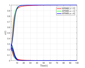
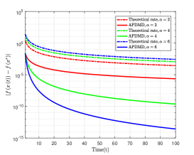
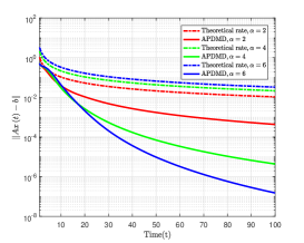
where , , . The objective function is convex (but not strongly convex) and smooth, and it is a very popular regularization in machine learning. Applying APDMD (39) with Kullback-Leibler divergence to address problem (58). (5) (left) shows the trajectories of estimates for of APDMD (39) versus time; (5) (middle) and (right) display the error of and respectively. The numerical results of gaps for objective function and equation constraints are in excellent agreement with our theoretical results, i.e., they both converge at the predicted rates.
Example 3.
Distributed Logistic regression: Consider a distributed problem (12) as follows:
| (59) |
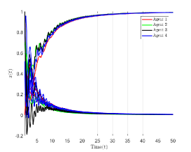
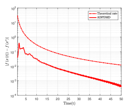
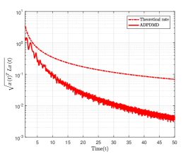
where . Setting and , , and . Note that the objective function in (59) is convex (but not strongly convex) and smooth, which satisfies the requirement of problem (12) in the smooth case. Applying ADPDMD (31) with 4 agents (connected as a ring) to solve problem (59), i.e., for agent 1, using Kullback-Leibler divergence; for agent 2, applying Itakura-Saito divergence; for agent 3, adopting projection operator of Sphere set; for agent 4, utilizing projection operator of half-space set. (6) (left) shows the trajectories of under ADPDMD (31) for problem (59) are uniformly convergent and globally asymptotically stable, i.e., ; (6) (middle) and (right) display the errors of and , respectively. The numerical results show and and all converge at the predicted rates.
Example 4.
Distributed quadratic programming: Consider a special case of DEMO (13) in the smooth case as follows:
| (60) |
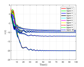
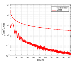
where , and is an auxiliary variable. Let , and be a positive semi-definite matrix generated by standard Gaussian distribution. Let every part be an agent, and 10 agents are connected as a ring. Applying the ADMD (36) to solve problem (60) and the experimental results are shown in (7). In (7) (left), the dual variable is uniformly convergent and globally asymptotically stable, i.e., ; (7) (middle and right) illustrate and of ADMD (36) are convergent at the predicted rates.
5.2 In the nonsmooth case
Example 5.
Nonnegative Basis Pursuit (NBP) in Khajehnejad et al. (2010): Take into account a NBP as follows:
| (61) |
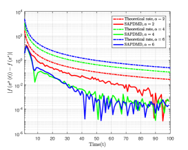
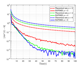
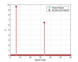
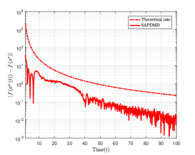
where and is an orthogonal Gaussian matrix. The objective function in (61) is convex (but not strongly convex) and nonsmooth as required. Applying the SAPDMD (39) and let to solve problem (61). (8) displays the reconstructed sparse signal of in the left, the error of in the middle, and the error of in the right. All parameters are complied with the requirement. The numerical results are in good accordance with our theoretical results, where the and are convergent at the predicted rates.
Example 6.
Distributed basis pursuit in row partition in Zhao et al. (2021): Take a distributed basis pursuit with row partition of sensing matrix as follows:
| (62) |
where ,
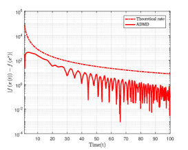
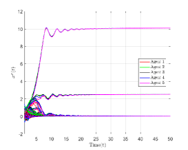
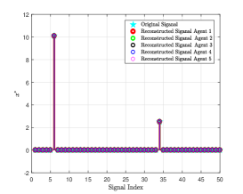
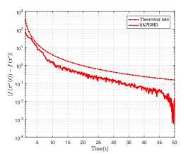
, . Note that, the problem (62) is convex (but not strongly convex) and nonsmooth and as a special case of DCCP (12) in the nonsmooth case. Setting , , , sparsity be and every acts as an agent, and 5 agents are connected as a ring. Applying the SADPDMD (50) with of affine set in (2.4) to solve the problem (62) and all parameters comply with the requirement. The numerical results are displayed in (9). As can be seen from (9) (left) that the variable is uniformly convergent and globally asymptotically stable, i.e., ; (8) (middle) shows that the SADPDMD can efficiently solve the problem (62) and reconstruct the original sparse signal; the result in (9) (middle) is in good accordance with our theoretical results, i.e., is convergent at the predicted rates.
Example 7.
Distributed basis pursuit in column partition in Zhao et al. (2021): Consider a distributed basis pursuit with column partition of sensing matrix as follows:
| (63) |
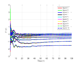
where , and is an auxiliary variable. Note that, the problem (63) is convex (but not strongly convex) and nonsmooth, which is a special case of DEMO (13). Letting , and , then . Let every part be an agent, and 10 agents are connected as a ring. Applying the ADMD (54) to solve the problem (63) and the experimental results are shown in (10). (10) (left) displays the dual variable is uniformly convergent and globally asymptotically stable, i.e., ; (10) (middle) describes that the SADMD (54) is able to efficiently solve the problem(63) and recover the sparse signal in a distributed way; (10) (right) illustrates of SADMD (54) converges at the predicted rates.
Acknowledgments and Disclosure of Funding
This work was supported in part by the National Key RD Program of China (No. 2018AAA0100101), in part by National Natural Science Foundation of China (Grant no. 61932006, 61772434) and in part by the Fundamental Research Funds for the Central Universities (Project No. XDJK2020TY003).
References
- Alimisis et al. (2020) Foivos Alimisis, Antonio Orvieto, Gary Bécigneul, and Aurelien Lucchi. A continuous-time perspective for modeling acceleration in riemannian optimization. In International Conference on Artificial Intelligence and Statistics, pages 1297–1307. PMLR, 2020.
- Alvarez (2000) Felipe Alvarez. On the minimizing property of a second order dissipative system in hilbert spaces. SIAM Journal on Control and Optimization, 38:1102–1119, 2000.
- Apidopoulos et al. (2018) Vassilis Apidopoulos, Jean-François Aujol, and Charles Dossal. The differential inclusion modeling fista algorithm and optimality of convergence rate in the case b . SIAM Journal on Optimization, 28:551–574, 2018.
- Attouch et al. (2019) Hedy Attouch, Zaki Chbani, and Hassan Riahi. Rate of convergence of the nesterov accelerated gradient method in the subcritical case . ESAIM: Control, Optimisation and Calculus of Variations, 25:2, 2019.
- Attouch et al. (2021) Hédy Attouch, Zaki Chbani, Jalal M. Fadili, and Hassan Riahi. Fast convergence of dynamical admm via time scaling of damped inertial dynamics. Journal of Optimization Theory and Applications, 2021.
- Aujol et al. (2020) Jean-François Aujol, Charles Dossal, and Aude Rondepierre. Convergence rates of the heavy-ball method for quasi-strongly convex optimization. 2020.
- Aujol et al. (2022) Jf Aujol, Charles Dossal, and Aude Rondepierre. Convergence rates of the heavy-ball method under the Łojasiewicz property. Mathematical Programming, pages 1–60, 2022.
- Balavoine et al. (2013) Aurele Balavoine, Christopher J. Rozell, and Justin K. Romberg. Convergence speed of a dynamical system for sparse recovery. IEEE Transactions on Signal Processing, 61:4259–4269, 2013.
- Banerjee et al. (2005) Arindam Banerjee, Srujana Merugu, Inderjit S Dhillon, Joydeep Ghosh, and John Lafferty. Clustering with bregman divergences. Journal of machine learning research, 6(10), 2005.
- Bauschke and Combettes (2011) Heinz H. Bauschke and Patrick L. Combettes. Convex analysis and monotone operator theory in hilbert spaces. In CMS Books in Mathematics, 2011.
- Beck and Teboulle (2003) Amir Beck and Marc Teboulle. Mirror descent and nonlinear projected subgradient methods for convex optimization. Operations Research Letters, 31(3):167–175, 2003.
- Bégout et al. (2015) Pascal Bégout, Jérôme Bolte, and Mohamed Ali Jendoubi. On damped second-order gradient systems. Journal of Differential Equations, 259(7):3115–3143, 2015.
- Bian and Chen (2014) Wei Bian and Xiaojun Chen. Neural network for nonsmooth, nonconvex constrained minimization via smooth approximation. IEEE Transactions on Neural Networks and Learning Systems, 25:545–556, 2014.
- Bian and Chen (2020) Wei Bian and Xiaojun Chen. A smoothing proximal gradient algorithm for nonsmooth convex regression with cardinality penalty. SIAM Journal on Numerical Analysis, 58:858–883, 2020.
- Bolte (2003) Jérôme Bolte. Sur des systèmes dynamiques dissipatifs de type gradient. applications en optimisation. 2003.
- Boyd et al. (2011) Stephen P. Boyd, Neal Parikh, Eric King wah Chu, Borja Peleato, and Jonathan Eckstein. Distributed optimization and statistical learning via alternating direction method of multipliers. Foundations and Trends in Machine Learning, 3:1–122, 2011.
- Boţ and Nguyen (2021) Radu Ioan Boţ and Dang-Khoa Nguyen. Improved convergence rates and trajectory convergence for primal-dual dynamical systems with vanishing damping. Journal of Differential Equations, 2021.
- Cabot and Frankel (2012) Alexandre Cabot and Pierre Frankel. Asymptotics for some semilinear hyperbolic equations with non-autonomous damping. Journal of Differential Equations, 252:294–322, 2012.
- Cabot and Paoli (2007) Alexandre Cabot and Laetitia Paoli. Asymptotics for some vibro-impact problems with a linear dissipation term. Journal de mathématiques pures et appliquées, 7:2030037–2030038, 2007.
- Chen (2012) Xiaojun Chen. Smoothing methods for nonsmooth, nonconvex minimization. Mathematical Programming, 134:71–99, 2012.
- Darbon and Langlois (2021) Jérôme Darbon and Gabriel Provencher Langlois. Accelerated nonlinear primal-dual hybrid gradient methods with applications to supervised machine learning. 2021.
- Diakonikolas and Jordan (2021) Jelena Diakonikolas and Michael I Jordan. Generalized momentum-based methods: A hamiltonian perspective. SIAM Journal on Optimization, 31(1):915–944, 2021.
- Elloumi et al. (2017) Mounir Elloumi, Ramzi May, and Chokri Mnasri. Asymptotic for a second order evolution equation with vanishing damping term and tikhonov regularization. arXiv: Optimization and Control, 2017.
- Fazlyab et al. (2017) Mahyar Fazlyab, Alec Koppel, Victor M. Preciado, and Alejandro Ribeiro. A variational approach to dual methods for constrained convex optimization. 2017 American Control Conference (ACC), pages 5269–5275, 2017.
- Feijer and Paganini (2010) Diego Feijer and Fernando Paganini. Stability of primal–dual gradient dynamics and applications to network optimization. Automatica, 46(12):1974–1981, 2010.
- Godsil and Royle (2001) Chris D. Godsil and Gordon F. Royle. Algebraic graph theory. In Graduate texts in mathematics, 2001.
- He et al. (2021) Xin He, Rong Hu, and Ya Ping Fang. Convergence rates of inertial primal-dual dynamical methods for separable convex optimization problems. SIAM Journal on Control and Optimization, 59(5):3278–3301, 2021.
- He et al. (2016) Xing He, Tingwen Huang, Junzhi Yu, Chuandong Li, and Chaojie Li. An inertial projection neural network for solving variational inequalities. IEEE transactions on cybernetics, 47(3):809–814, 2016.
- He et al. (2017) Xing He, Daniel WC Ho, Tingwen Huang, Junzhi Yu, Haitham Abu-Rub, and Chaojie Li. Second-order continuous-time algorithms for economic power dispatch in smart grids. IEEE Transactions on Systems, Man, and Cybernetics: Systems, 48(9):1482–1492, 2017.
- Hopfield and Tank (1986) John J. Hopfield and David W. Tank. Computing with neural circuits: a model. Science, 233 4764:625–33, 1986.
- Kennedy and Chua (1988) Michael Peter Kennedy and Leon O Chua. Neural networks for nonlinear programming. IEEE Transactions on Circuits and Systems, 35(5):554–562, 1988.
- Khajehnejad et al. (2010) M Amin Khajehnejad, Alexandros G Dimakis, Weiyu Xu, and Babak Hassibi. Sparse recovery of nonnegative signals with minimal expansion. IEEE Transactions on Signal Processing, 59(1):196–208, 2010.
- Kovachki and Stuart (2021) Nikola B Kovachki and Andrew M Stuart. Continuous time analysis of momentum methods. Journal of Machine Learning Research, 22(17):1–40, 2021.
- Krichene et al. (2015) Walid Krichene, Alexandre M. Bayen, and Peter L. Bartlett. Accelerated mirror descent in continuous and discrete time. In Conference on Neural Information Processing Systems, 2015.
- Krichene et al. (2016) Walid Krichene, Alexandre Bayen, and Peter Bartlett. A Lyapunov Approach to Accelerated First-Order Optimization in Continuous and Discrete Time. PhD thesis, University of California, Berkeley, 2016.
- Lin et al. (2020) Zhouchen Lin, Huan Li, and Cong Fang. Accelerated optimization for machine learning. Springer, 2020.
- Liu et al. (2017) Qingshan Liu, Shaofu Yang, and Jun Wang. A collective neurodynamic approach to distributed constrained optimization. IEEE Transactions on Neural Networks and Learning Systems, 28:1747–1758, 2017.
- Luo (2021) Hao Luo. Accelerated primal-dual methods for linearly constrained convex optimization problems. 2021.
- Nandwani et al. (2019) Yatin Nandwani, Abhishek Pathak, Mausam, and Parag Singla. A primal dual formulation for deep learning with constraints. In In Advances in Neural Information Processing Systems, 2019.
- Nesterov (2005) Yurii Nesterov. Smooth minimization of non-smooth functions. Mathematical Programming, 103:127–152, 2005.
- O’Connor and Vandenberghe (2014) Daniel O’Connor and Lieven Vandenberghe. Primal-dual decomposition by operator splitting and applications to image deblurring. SIAM Journal on Imaging Sciences, 7:1724–1754, 2014.
- Parikh and Boyd (2014) Neal Parikh and Stephen P. Boyd. Proximal algorithms. Foundations and Trends in optimization, 1:127–239, 2014.
- Polyak (1964) Boris Polyak. Some methods of speeding up the convergence of iteration methods. Ussr Computational Mathematics and Mathematical Physics, 4:1–17, 1964.
- Qu and Li (2019) Guannan Qu and Na Li. On the exponential stability of primal-dual gradient dynamics. IEEE Control Systems Letters, 3:43–48, 2019.
- Rockafellar (1970) R. Tyrrell Rockafellar. Convex analysis. In Princeton Landmarks in Mathematics and Physics, 1970.
- Su et al. (2016) Weijie J. Su, Stephen P. Boyd, and Emmanuel J. Candès. A differential equation for modeling nesterov’s accelerated gradient method: Theory and insights. In Journal of Machine Learning Research, 2016.
- Tiapkin and Gasnikov (2022) Daniil Tiapkin and Alexander Gasnikov. Primal-dual stochastic mirror descent for mdps. In International Conference on Artificial Intelligence and Statistics, pages 9723–9740. PMLR, 2022.
- Wibisono et al. (2016) Andre Wibisono, Ashia C. Wilson, and Michael I. Jordan. A variational perspective on accelerated methods in optimization. Proceedings of the National Academy of Sciences, 113:E7351 – E7358, 2016.
- Wilson et al. (2021) Ashia C Wilson, Ben Recht, and Michael I Jordan. A lyapunov analysis of accelerated methods in optimization. Journal of Machine Learning Research, 22:113–1, 2021.
- Yi et al. (2016) Peng Yi, Yiguang Hong, and Feng Liu. Initialization-free distributed algorithms for optimal resource allocation with feasibility constraints and application to economic dispatch of power systems. Automatica, 74:259–269, 2016.
- Zeng et al. (2018) Xianlin Zeng, Peng Yi, Yiguang Hong, and Lihua Xie. Distributed continuous-time algorithms for nonsmooth extended monotropic optimization problems. SIAM Journal on Control and Optimization, 56(6):3973–3993, 2018.
- Zeng et al. (2022) Xianlin Zeng, Jinlong Lei, and Jie Chen. Dynamical primal-dual accelerated method with applications to network optimization. IEEE Transactions on Automatic Control, pages 1–1, 2022. doi: 10.1109/TAC.2022.3152720.
- Zhang and Xiao (2017) Yuchen Zhang and Lin Xiao. Stochastic primal-dual coordinate method for regularized empirical risk minimization. Journal of Machine Learning Research, 18(84):1–42, 2017. URL http://jmlr.org/papers/v18/16-568.html.
- Zhao et al. (2018) You Zhao, Xing He, Tingwen Huang, and Junjian Huang. Smoothing inertial projection neural network for minimization lp-q in sparse signal reconstruction. Neural networks, 99:31–41, 2018.
- Zhao et al. (2021) You Zhao, Xiao-Fei Liao, Xing He, and Rongqiang Tang. Centralized and collective neurodynamic optimization approaches for sparse signal reconstruction via -minimization. IEEE Transactions on Neural Networks and Learning Systems, PP, 2021.
- Zhu and Hazan (2016) Zeyuan Allen Zhu and Elad Hazan. Optimal black-box reductions between optimization objectives. In Conference on Neural Information Processing Systems, 2016.